Potential of radio telescopes as high-frequency gravitational wave detectors

Abstract

In the presence of magnetic fields, gravitational waves are converted into photons and vice versa. We demonstrate that this conversion leads to a distortion of the cosmic microwave background (CMB), which can serve as a detector for MHz to GHz gravitational wave sources active before reionization. The measurements of the radio telescope EDGES can be cast as a bound on the gravitational wave amplitude, $h_{c}<10^{-21}(10^{-12})$ at 78 MHz, for the strongest (weakest) cosmic magnetic fields allowed by current astrophysical and cosmological constraints. Similarly, the results of ARCADE 2 imply $h_{c}<10^{-24}(10^{-14})$ at $3-30$ GHz. For the strongest magnetic fields, these constraints exceed current laboratory constraints by about seven orders of magnitude. Future advances in 21cm astronomy may conceivably push these bounds below the sensitivity of cosmological constraints on the total energy density of gravitational waves.

Gravitational waves (GWs) produced in the early Universe Maggiore:2018sht ; Caprini:2018mtu can traverse cosmic distances without experiencing any interactions, making them a unique probe of very high energy physics. Since the comoving Hubble horizon grows with time, GWs produced at energies around the scale of grand unification have frequencies in the MHz and GHz regime today, far beyond the reach of the laser interferometers LIGO, VIRGO or KAGRA. See REECE1984341 ; Cruise:2006zt ; Akutsu:2008qv ; Ito:2020wxi ; Cruise_2012 ; Ejlli:2019bqj for some existing laboratory bounds at these frequencies.

Here we focus on searching for high-frequency GWs exploiting the (inverse) Gertsenshtein effect Gertsenshtein ; Boccaletti1970 , which describes the conversion of GWs into photons in the presence of a magnetic field (see e.g. DeLogi:1977qe ; Raffelt:1987im ; Macedo:1984di ; Fargion:1995mm ; Dolgov:2012be ; Cruise_2012 ; Ejlli:2019bqj ; Ejlli:2020fpt ). As an immediate consequence of general relativity and classical electromagnetism, this is a purely SM process. Involving gravity, the conversion probability is extremely small which may, however, be compensated by considering a ‘detector’ of cosmological size. In fact, magnetic fields with cosmological correlation lengths might well permeate our Universe with certain astrophysical observations strongly suggesting a lower limit of order $10^{-16}\,\mathrm{G}$ Neronov:1900zz ; Tavecchio:2010mk ; Takahashi:2013lba , and the CMB setting an upper bound in the pG-nG range Jedamzik:2018itu ; Ade:2015cva ; Pshirkov:2015tua . See Durrer:2013pga for a comprehensive review.

The pioneering study PhysRevLett.74.634 proposed the inverse Gertsenshtein effect in cosmic magnetic fields to search for GWs but neglected the plasma mass of photons, as pointed out in Ref. Cillis:1996qy . The idea was revisited in Ref. Pshirkov:2009sf suggesting an observable effect, however as noted in Dolgov:2012be decoherence effects were not correctly accounted for. More recently Fujita:2020rdx studied the production of GWs from CMB photons. In this letter, we focus on CMB distortions arising from the Gertsenshtein effect during the dark ages, i.e. the period between recombination and reionization. Due to the small fraction of free electrons in this period, the effective plasma mass of the photons is suppressed, increasing the conversion probability between GWs and photons. Taking into account inhomogeneities in the thermal plasma and in the cosmic magnetic fields, we demonstrate that existing measurements of the Rayleigh-Jeans tail of the CMB spectrum, performed e.g. by ARCADE 2 Fixsen_2011 and by EDGES Bowman:2018yin , can be translated into constraints on GWs in the MHz-GHz regime. These are competitive with, or even exceed, current laboratory constraints, depending on the assumptions on the cosmic magnetic fields.

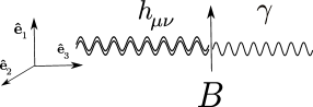
Figure 1: The Gertsenshtein effect.

I The Gertsenshtein effect

Calculating the conversion rate for this oscillation process requires solving Maxwell’s equations for the vector potential, $A^{\mu}$, describing the electromagnetic radiation, together with the linearized Einstein’s equations for the metric $g_{\mu\nu}=\eta_{\mu\nu}+h_{\mu\nu}$, in which $h_{\mu\nu}$ describes the GWs. In this work we will adopt $\eta_{\mu\nu}=\text{diag}(+---)$ and work with natural Heaviside-Lorentz units ($\hbar=c=1$), except in this section where we keep fundamental constants explicitly to emphasize that the Gertsenshtein effect is a classical phenomenon.

Let us ignore the Universe expansion first and consider a GW propagating in the $\mathbf{\hat{e}_{3}}$ direction inside a fixed box of size $\Delta\ell$ that contains a uniform transverse magnetic field, $B$, and a non-negligible uniform density of free electrons, $n_{e}$. Without loss of generality, we assume that the magnetic field points in the $\mathbf{\hat{e}_{1}}$ direction. See Fig. 1. In this coordinate system we introduce $h_{\times}=h^{12}=h^{21}$ and $A_{\times}=A^{1}$ as well as $h_{+}=-h^{22}=h^{11}$ and $A_{+}=-A^{2}$. This is because the aforementioned equations can be elegantly cast as Dolgov:2012be ; Raffelt:1987im  

$$\left(\Box+\omega^{2}_{\text{pl}}/c^{2}\right)A_{\lambda}=-B\partial_{\ell}h_{\lambda}\,, \Box h_{\lambda}=\kappa^{2}B\partial_{\ell}A_{\lambda}\,,$$ (1)

where $\lambda\in\{+,\times\}$, $\ell$ is the third component, $\Box=\partial_{t}^{2}/c^{2}-\partial_{\ell}^{2}$, $\kappa=\left(16\pi G\right)^{1/2}/c^{2}$. We include the plasma frequency $\omega_{\text{pl}}=\sqrt{e^{2}n_{e}/m_{e}}$, which acts as an effective mass term and gives electromagnetic waves of frequency $\omega$ a refractive index $\mu=\sqrt{1-\omega_{\text{pl}}^{2}/\omega^{2}}$ when $B\to 0$. Eq. (1) also applies for arbitrary uniform fields with $B$ interpreted as the corresponding transverse component. See the supplementary material for more details. Assuming a plane wave traveling in the positive direction with $\omega\geq\omega_{\text{pl}}$, the exact solution of Eqs. (1) (see also Ejlli:2020fpt ) can be written as

$$\psi(t,\ell)\equiv\begin{pmatrix}\sqrt{\mu}\,\,A_{\lambda}\\ \frac{1}{\kappa}\,h_{\lambda}\end{pmatrix}=e^{-i\omega t}e^{iK\ell}\psi(0,0)\,,\,$$ (2)

with $K$ being the Hermitian matrix

$$K=\begin{pmatrix}\frac{\mu}{c}\sqrt{\omega^{2}+\left(\frac{\kappa B}{1+\mu}\right)^{2}}\,&-i\frac{\sqrt{\mu}\,\kappa B}{1+\mu}\\ i\frac{\sqrt{\mu}\,\kappa B}{1+\mu}&\frac{1}{c}\sqrt{\omega^{2}+\left(\frac{\kappa B}{1+\mu}\right)^{2}}\end{pmatrix}\,.$$ (3)

It is convenient to introduce $\psi$ because its magnitude, $|\psi(t,\ell)|^{2}$ , is conserved. This easily follows from the unitarity of the matrix ${\cal U(\ell)}=e^{iK\ell}$. In particular, $\psi(0,0)=(0,h_{\lambda,0}/\kappa)$ for a pure GW state entering the box, and consequently $\psi(t,\Delta\ell)=e^{-i\omega t}\left({\cal U}_{12}(\Delta\ell),{\cal U}_{22}(\Delta\ell)\right)h_{\lambda,0}/\kappa$ after leaving the box. Since $|{\cal U}_{12}(\Delta\ell)|^{2}+|{\cal U}_{22}(\Delta\ell)|^{2}=1$, the quantity $P(\Delta\ell)\equiv|{\cal U}_{12}(\Delta\ell)|^{2}$ can be interpreted as the probability of GW conversion after traversing a distance $\Delta\ell$. Simple algebra shows

$$P(\Delta\ell)=|K_{12}|^{2}\,\ell_{\text{osc}}^{2}\,\sin^{2}(\Delta\ell/\ell_{\text{osc}})\,,$$ (4)

with $\ell_{\text{osc}}^{-1}=\sqrt{\omega^{2}(1-\mu)^{2}/c^{2}+\kappa^{2}B^{2}}/2$. These expressions reduce to the approximated formulae previously found (see e.g. Raffelt:1987im ; Ejlli:2018hke ).

Although cosmic magnetic fields are not expected to be perfectly homogeneous, coherent oscillations take place in highly homogeneous patches, for which $\ell_{\text{osc}}\ll\Delta\ell$ and therefore $P(\Delta\ell)=|K_{12}|^{2}\ell_{\text{osc}}^{2}/2$ on average. Taking into account inhomogeneities in $n_{e}$  and $B$, the coherence of the $g\leftrightarrow\gamma$ oscillations is lost on distances larger than $\Delta\ell$, that is, the smallest distance on which $B$ and $n_{e}$ are uniform. Denoting the total distance traveled by the GW as $D$, this corresponds to traversing $N=D/\Delta\ell$ independent regions with a conversion probability $P(\Delta\ell)$ each. As long as $N\cdot P(\Delta\ell)\ll 1$, this gives a total conversion probability of $P(D)=D|K_{12}|^{2}\ell_{\text{osc}}^{2}/(2\Delta\ell)$  Cillis:1996qy ; Pshirkov:2009sf , corresponding to an average conversion rate (i.e. probability per time)  given by

$$\langle\Gamma_{g\leftrightarrow\gamma}\rangle=\frac{c\,|K_{12}|^{2}\ell_{\text{osc}}^{2}}{2\Delta\ell}\,.$$ (5)

In the supplementary material we demonstrate that this simple estimate correctly captures the essential features of a more involved computation based on the expected power spectrum of the magnetic field. Note that any additional inhomogeneities would further enhance the conversion rate by limiting the coherence of the $g\leftrightarrow\gamma$ oscillations.

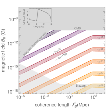
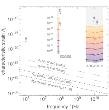
Figure 2: Left: Parameter space for cosmic magnetic fields today. Gray shaded areas show the exclusion discussed in the text. The solid (dashed) colored curves indicate contour lines for the re-scaled conversion probability, $(T_{0}/\omega_{0})^{2}{\cal P}$. See Eqs. (6) and (7). Right: Upper bounds on the stochastic GW background derived from ARCADE2 and EDGES (this work), compared to existing laboratory bounds from a) superconducting parametric converter REECE1984341 , b) waveguide Cruise:2006zt , c) 0.75 m interferometer Akutsu:2008qv , d) magnon detector Ito:2020wxi and e) magnetic conversion detector Cruise_2012 . The solid lines indicate the allowed parameter space for cosmic magnetic fields, as given in the left panel. The dashed lines mark the $N_{\text{eff}}$ constraint for broad GW spectra and for a peaked spectrum with $\Delta\omega/\omega=10^{-3}$. For reference, the dotted lines indicate $\rho_{g}=\rho_{c}$.

We now include the effect of the Universe expansion during the dark ages. This is the period between photon decoupling and reionization, $z_{\text{dec}}\simeq 1100\gtrsim z\gtrsim z_{\text{rei}}\simeq 10$, beginning with the formation of the CMB and ending when the first stars were formed. During this time, the refractive index of MHz-GHz CMB photons is determined by the tiny electron density, with the contributions of neutral hydrogen, helium and birefringence being subdominant Chen:2013gva ; Kunze:2015noa ; Mirizzi:2009iz . This allows us to adopt Eq (5), after a few modifications. The conversion probability in an adiabatic expanding Universe is simply the line-of-sight integral of the rate

$${\cal P}\equiv\int_{l.o.s.}\langle\Gamma_{g\leftrightarrow\gamma}\rangle dt=\int^{z_{\text{ini}}}_{0}\frac{\langle\Gamma_{g\leftrightarrow\gamma}\rangle}{(1+z)\,H}dz\,,$$ (6)

where we use null-geodesics $Hdt=dT/T=dz/(1+z)$. Also, $z_{\text{ini}}\leq z_{\text{dec}}$ is an initial condition to be specified below and $H=H_{\text{dec}}\left(T/T_{\text{dec}}\right)^{3/2}$ is the Hubble parameter during the dark ages, which are matter dominated. Furthermore, the average magnetic energy density of the Universe $\rho_{B}=B^{2}/2$ redshifts as $\rho_{B}=\rho_{B0}\left(1+z\right)^{4}$ . Additionally, such a field is associated with a coherence length, $\lambda_{B}=\lambda^{0}_{B}/(1+z)$, because it is not expected to be homogeneous everywhere. Concerning these two quantities we emphasize three important facts here and refer the reader to Durrer:2013pga for a more comprehensive discussion: i) a recent CMB analysis gives $B_{0}\lesssim 47\,\mathrm{pG}$ Jedamzik:2018itu ii) Blazar observations strongly suggest a lower limit on $B_{0}$ Caprini:2015gga because otherwise their gamma-ray spectra can not be explained under standard cosmological assumptions Neronov:1900zz ; Tavecchio:2010mk ; Takahashi:2013lba ; Chen:2014rsa , and iii) magnetohydrodynamic turbulence damps out large magnetic fields at small distances, imposing an additional (theoretical) upper limit Durrer:2013pga . Fig. 2 show these constraints.

In addition, the electron number density during this epoch is $n_{e}(z)=n_{b0}(1+z)^{3}X_{e}(z)$, where $n_{b0}=0.251\,\mathrm{m^{-3}}$ is the baryon number density today Aghanim:2018eyx and $X_{e}(z)$ is the ionization fraction, taking values $1,\,0.68,\,0.0002$ and $0.15$ at $z=0,\,10,\,20$ and $1100$, respectively . This gives plasma frequencies today, $\omega_{\text{pl},0}$, lying in the Hz range, which allows us to take $1-\mu(z)=(1+z)X_{e}(z)\omega_{\text{pl},0}^{2}/(2\omega_{0}^{2})\ll 1$, for waves of frequency $\omega=\omega_{0}(1+z)$ with $\omega_{0}\sim$ GHz. Moreover, $B_{0}\lesssim 47\,\mathrm{pG}$ results in the oscillation length being numerically dominated by the plasma frequency so that $\ell_{\text{osc}}^{-1}=(1+z)^{2}X_{e}(z)\omega_{\text{pl},0}^{2}/(4\omega_{0}c)$. This gives $\ell_{\text{osc}}\ll 1\,\mathrm{pc}\ll\Delta\ell$, as anticipated above. Here, in order to account for electron inhomogeneities we conservatively take $\Delta\ell=\Delta\ell_{0}/(1+z)$ to be given by $\Delta\ell_{0}=\text{min}[\lambda_{\text{EQ}},\lambda_{B}^{0}]$ where $\lambda_{EQ}/(2\pi)=95\,\mathrm{Mpc}$ is the characteristic comoving scale for the onset of structure formation (corresponding to the perturbation mode entering the horizon at matter-radiation equality). Putting all this together, we obtain

$${\cal P}\simeq\,6.3\times 10^{-19}\left(\frac{B_{0}}{\text{nG}}\right)^{2}\left(\frac{\omega_{0}}{T_{0}}\right)^{2}\left(\frac{\text{Mpc}}{\Delta\ell_{0}}\right)\left(\frac{{\cal I}(z_{\text{ini}})}{10^{6}}\right),$$ (7)

with $T_{0}/(2\pi)=2.725\leavevmode\nobreak\ \text{K}/(2\pi)=56.78$ GHz and ${\cal I}(z_{\text{ini}})=\int_{0}^{z_{\text{ini}}}dz\,(1+z)^{-3/2}X_{e}^{-2}(z)$. The left panel of Fig. 2 displays contours of $(T_{0}/\omega_{0})^{2}{\cal P}$ in the parameter space of cosmic magnetic fields. The inset shows ${\cal I}^{\prime}(z_{\text{ini}})$, explaining the weak redshift-dependence of ${\cal I}(z_{\text{ini}})$, with the largest contribution arising from $z\sim 10$.

II CMB Distortions

The CMB photon distribution, $f_{\gamma}(\omega,T)$, retains its equilibrium form during the dark ages, i.e. is given by a black-body spectrum, $f_{\text{eq}}=1/(e^{\omega/T}-1)$ with $\omega/T=\omega_{0}/T_{0}$. Our aim here is to calculate deviations from such a spectrum, $\delta f_{\gamma}=f_{\gamma}-f_{\text{eq}}$.

The spectrum of GWs is commonly characterized by $\Omega_{\text{GW}}$, which parametrizes the corresponding energy density per logarithmic frequency bin. This quantity can be used to introduce – in an analogous manner to $f_{\gamma}$– the distribution function for GWs, $f_{g}$. More precisely, in terms of it, the energy density is given by

$$\rho_{g}(T)=\int\frac{d\ln\omega}{\pi^{2}}\,\omega^{4}f_{g}\equiv\rho_{c}(T)\int d\ln\omega\,\,\Omega_{\text{GW}}\left(\frac{\omega}{2\pi},T\right),$$ (8)

with $\rho_{c}(T)$ denoting the Universe total energy density.

Both distributions satisfy the Boltzmann equation $\hat{L}f_{\gamma/g}=\pm\langle\Gamma_{g\leftrightarrow\gamma}\rangle(f_{g}-f_{\gamma})$, where $\hat{L}\equiv\partial_{t}-H\omega\partial_{\omega}=-H\left(T\partial_{T}+\omega\partial_{\omega}\right)$ is the corresponding Lioville operator. Its solution leads to

$$\delta f_{\gamma}(\omega_{0},T_{0})=\left(f_{g}(\omega_{\text{ini}},T_{\text{ini}})-f_{\text{eq}}\right){\cal P}+{\cal O}({\cal P}^{2})\,,$$ (9)

with ${\cal P}$ defined as in Eq. (6). We solve the Boltzmann equations from an initial temperature $T=T_{\text{ini}}$ – when the photon distribution is a black-body spectrum, i.e $f_{\gamma}(\omega,T_{\text{ini}})=f_{\text{eq}}(\omega/T_{\text{ini}})$ – until today. If decoupling is prior to the GW emission, the latter fixes $T_{\text{ini}}$. Otherwise, we set $T_{\text{ini}}=T_{\text{dec}}$ because the ionization fraction sharply drops after $z\sim z_{\text{dec}}$ rendering any prior contribution negligible. This is illustrated in the inset of Fig. 2 (left panel), which also shows that the conversion rate is anyways largely insensitive to the precise value of $T_{\text{ini}}$.

Eq. (9) can alternatively be derived by considering the density-matrix formalism. In that case case, $f_{\gamma}$ and $f_{g}$ are proportional to the diagonal entries of such a matrix, which evolves by means of the Hamiltonian associated with Eq. (3). See the supplementary material for details. The fact that using both methods we obtain the same result –i.e. Eq. (9)– is reassuring and indicates that decoherence effects are properly taken into account Dolgov:2012be . Due to this as well as the way we treat inhomogeneities, our results differ from those of Pshirkov:2009sf .

III Constraints on the stochastic GW background

In this letter we focus on the Rayleigh-Jeans part of the CMB, i.e. $\omega\ll T$ implying $f_{\text{eq}}\simeq T/\omega$. In this regime, a subdominant GW contribution to the total radiation energy density is compatible with $f_{g}\gg f_{\gamma}\leavevmode\nobreak\$, and can thus produce an enhancement of the low-frequency CMB tail through the first term of Eq. (9). More precisely, the assumption $f_{g}>f_{\gamma}$ translates to $\Omega_{\text{GW}}/\Omega_{\gamma}>15/\pi^{4}(\omega/T)^{3}$ as can be seen by rewriting Eq. (8) as $\Omega_{\text{GW}}=\omega^{4}f_{g}\left(\omega,T\right)/(\pi^{2}\rho_{c})=(15/\pi^{4})\,\left(\omega/T\right)^{4}f_{g}(\omega,T)\,\Omega_{\gamma}\,$ with $\Omega_{\gamma}=\rho_{\gamma}/\rho_{c}=\pi^{2}T^{4}/(15\,\rho_{c})$. Even a scale-invariant GW spectrum as small as $\Omega_{\text{GW}}\simeq 10^{-15}$ implies $f_{g}>f_{\gamma}$ at e.g. $\omega/T\simeq 10^{-3}$.

With $\omega\ll T$ and $f_{g}\gg f_{\gamma}$, Eq. (9) reads

$$\frac{\delta f_{\gamma}}{f_{\gamma}}\left(\omega_{0},T_{0}\right)=\frac{\pi^{4}}{15}\left(\frac{T}{\omega}\right)^{3}{\cal P}\,\frac{\Omega_{\text{GW}}}{\Omega_{\gamma}}\,.$$ (10)

For a given detector sensitivity $\delta f_{\gamma}/f_{\gamma}$ and a given value of the conversion probability ${\cal P}$, relation (10) sets stringent bounds on the GW spectrum, which can be expressed in terms of the characteristic strain by means of Maggiore:1900zz

$$h_{c}=\left(\frac{3H_{0}^{2}}{4\pi^{2}}\Omega_{\text{GW}}f^{-2}\right)^{1/2}\,.$$ (11)

This is related to the one-sided power spectral density $S_{h}$ as $h_{c}=\sqrt{fS_{h}(f)}$. Fig. 2 contrasts the resulting constraints with existing bounds in the literature.

$N_{\text{eff}}$ bound.

GWs contribute to the energy budget of the Universe in the form of radiation and are as such constrained by the BBN and CMB bounds on the effective number of massless degrees of freedom $N_{\text{eff}}$ Pagano:2015hma ,

$$\rho_{g}(T)\leq\frac{7}{8}\left(\frac{4}{11}\right)^{4/3}\Delta N_{\text{eff}}\,\rho_{\gamma}(T)\,,$$ (12)

with $\Delta N_{\text{eff}}\lesssim 0.1$ Cyburt:2015mya ; Aghanim:2018eyx . For a spectrum $\Omega_{\text{GW}}$ which is approximately scale invariant between $f_{\text{min}}$ and $f_{\text{max}}$ with $\ln(f_{\text{max}}/f_{\text{min}})\sim{\cal O}(1)$, this implies

$$\frac{\Omega_{\text{GW}}}{\Omega_{\gamma}}\lesssim\frac{7}{8}\left(\frac{4}{11}\right)^{4/3}\Delta N_{\text{eff}}\,,$$ (13)

whereas for a narrow spectrum peaked at $\tilde{\omega}$ with width $\Delta\tilde{\omega}\lesssim\tilde{\omega}$ this bound is relaxed by a factor $(\tilde{\omega}/\Delta\tilde{\omega})$. Note that this bound applies only to GWs present already at CMB decoupling.

Probing the Rayleigh-Jeans tail of the CMB spectrum.

Below $\omega_{0}/T_{0}\sim 10^{-2}$, galactic foregrounds dominate the radio sky. Here we focus on the results reported by ARCADE2 Fixsen_2011 which covers the sweet spot of the low-frequency Rayleigh-Jeans spectrum before galactic foregrounds become important ($f=\omega_{0}/(2\pi)=3$, 8, 10, 30 and 90 GHz) and by EDGES Bowman:2018yin , which is a recent measurement of the global 21cm absorption signal at 78 MHz.

ARCADE2 was a balloon experiment equipped with a radio receiver measuring the black body temperature of sky Fixsen_2011 . The cleanest frequency band is around 10 GHz enabling a mK resolution, $\delta f_{\gamma}/f_{\gamma}=\delta T/T_{\text{CMB}}\lesssim 4\times 10^{-4}$ at $\omega_{0}/T_{0}\simeq 0.18$. At smaller frequencies, ARCADE2 observed a significant radio excess beyond the expected galactic foreground whose origin remains an open question (see e.g. Seiffert_2011 ; Feng:2018rje ). Assuming that this excess is entirely astrophysical, we can impose an upper bound on an additional contribution from a stochastic GW background using the 3, 8, 10 and 30 GHz frequency bands. In Fig 2, these frequencies are marked by crosses, the solid lines connecting them serve only to guide the eye.

Recently, the first observation of the global (i.e. sky-averaged) 21cm absorption signal was reported by the EDGES collaboration Bowman:2018yin . The absorption feature was found to be roughly twice as strong as previously expected, which if true, would indicate that either the primordial gas was significantly colder or the radiation background was significantly hotter than expected. Conservatively, we may assume that the deviation from the expected value is due to foreground contamination, and place a bound on any stochastic GW background by using $\delta f_{\gamma}/f_{\gamma}\lesssim 1$ at $\omega/T=1.4\times 10^{-3}$ (78 MHz). The width of the observed absorption feature (19 MHz) determines the width of the frequency coverage.

IV Discussion

Cosmological sources of GWs typically produce stochastic GW backgrounds with a frequency roughly related to the comoving Hubble horizon at the time of production. Processes in the very early Universe at energy scales far beyond the reach of colliders thus generically produce GWs in the MHz and GHz regime. Despite the large amount of redshift, these violent processes can produce sizeable GW signals, saturating the $N_{\text{eff}}$ bound (12). Some examples are axion inflation Barnaby:2010vf , metastable cosmic strings Buchmuller:2019gfy and evaporating light primordial black holes Anantua:2008am ; Dong:2015yjs . Further significant contributions may be expected from preheating Dolgov:1989us ; Traschen:1990sw ; Kofman:1994rk ; Kofman:1997yn ; Figueroa:2017vfa and first order phase transitions occurring above $10^{7}$ GeV Witten:1984rs ; Hogan:1986qda ; Punturo:2010zz ; Hild:2010id ; Evans:2016mbw . The sensitivity of radio telescopes can however not yet compete with the cosmological $N_{\text{eff}}$ bound, unless one considers essentially monochromatic signals (which may arise e.g. from large monochromatic scalar perturbations Bugaev_2010 ; Saito_2010 ).

Since the dominant contribution to ${\cal P}$ arises around reionization, a particularly interesting target are GW sources active around $10\lesssim z\lesssim 10^{3}$, which would not be constrained by the $N_{\text{eff}}$ bound. During the dark ages, there is no generic reason to expect GW production in the GHz regime but there are models which predict such a signal for suitable parameter choices. For example, mergers of light primordial black holes in this epoch (with masses of about $10^{-9..-7}\leavevmode\nobreak\ M_{\odot}$) would result in GHz GW signals today Maggiore:1900zz , see Raidal_2019 ; Gow_2020 for a discussion of possible rates. Superradiant axion clouds around spinning black holes yield an essentially monochromatic GW signal with $f\lesssim$ MHz Arvanitaki:2009fg ; Arvanitaki:2010sy ; Arvanitaki:2012cn , with higher frequency possible when considering primordial black holes with masses below the Chandrasekhar limit.

We emphasize that the use of radio telescopes allows to search for GWs in a wide frequency regime. While the absence of any excess radiation can already constrain some models under the assumption of strong cosmic magnetic fields, the potential of this method will truly unfold with further improvements in the sensitivity of radio telescopes –driven in particular by the advances in 21cm cosmology– or in the case of a positive detection of excess radiation.

An example of future advances in radio astronomy is the case of the Square Kilometer Array (SKA). Assuming an effective area per antenna temperature of at least $10^{2}\,\mathrm{m^{2}/K}$ Braun:2019gdo in the $0.1-10$ GHz range, a few hours of observation will lead to sensitivities in the ballpark of $\mathrm{\mu Jy}$, which must be compared against CMB fluxes of at least $10^{3}\,\mathrm{Jy}$. SKA measurements are thus very promising although sufficient foreground subtraction will be extremely challenging.

Acknowledgments.

It is a pleasure to thank Nancy Aggarwal, Sebastien Clesse, Mike Cruise, Hartmut Grote and Francesco Muia for insightful discussions on the Gertsenshtein effect and high-frequency GW sources at the ICTP workshop “Challenges and opportunities of high-frequency gravitational wave detection”. Likewise, we would also like to thank Torsten Bringmann, Damian Ejlli, Kohei Kamada and Kai Schmidt-Hoberg. This work was partially funded by the Deutsche Forschungsgemeinschaft under Germany’s Excellence Strategy - EXC 2121 “Quantum Universe” - 390833306. C.G.C. is supported by the Alexander von Humboldt Foundation.

V Supplementary material

V.1 The wave equation

Gravitational radiation sourcing electromagnetic waves.

Maxwell’s equations in curved space-time can be written as

$$0=\nabla_{\nu}F^{\mu\nu}+\frac{1}{c}j^{\mu}=\frac{1}{\sqrt{-g}}\partial_{\nu}\left(\sqrt{-g}F^{\mu\nu}\right)+\frac{1}{c}j^{\mu}\,,$$ (14)

where $j^{\mu}$ and $F^{\mu\nu}$ are respectively the electromagnetic current and strength-field tensor in Lorentz-Heaviside units. In this work $\eta_{\mu\nu}=\text{diag}(+---)$. For metric fluctuations describing a gravitational wave, $g_{\mu\nu}=\eta_{\mu\nu}+h_{\mu\nu}$, we have $\partial_{\nu}\sqrt{-g}/\sqrt{-g}=g^{\rho\sigma}\partial_{\nu}g_{\rho\sigma}/2=\partial_{\nu}\left(\eta^{\rho\sigma}h_{\rho\sigma}\right)/2+{\cal O}(h^{2})$. Moreover, for an electromagnetic wave determined by the vector potential, $A^{\mu}$, and propagating in the presence of a uniform and constant magnetic field, $F^{\text{ext}}_{\mu\nu}$, the part of the electromagnetic tensor linear in only $A$ or $h$ is

$$F^{\mu\nu}\supseteq\left(\eta^{\mu\lambda}\partial_{\lambda}A^{\nu}-\eta^{\nu\lambda}\partial_{\lambda}A^{\mu}\right)+\left(\eta^{\alpha\mu}\eta^{\beta\nu}-h^{\alpha\mu}\eta^{\beta\nu}-\eta^{\alpha\mu}h^{\beta\nu}\right)F^{\text{ext}}_{\alpha\beta}\,.$$ (15)

Notice that $F^{\text{ext}\,{\alpha\beta}}$ varies due to the fluctuating metric in contrast to $F^{\text{ext}}_{\alpha\beta}$, which does not change. Then, Eq. (14) to leading order is

$$\eta^{\mu\lambda}\partial_{\lambda}\partial_{\nu}A^{\nu}-\eta^{\nu\lambda}\partial_{\nu}\partial_{\lambda}A^{\mu}-\partial_{\nu}h^{\alpha\mu}\eta^{\beta\nu}F^{\text{ext}}_{\alpha\beta}-\eta^{\alpha\mu}\partial_{\nu}h^{\beta\nu}F^{\text{ext}}_{\alpha\beta}+\frac{1}{2}\partial_{\nu}\left(\eta^{\rho\sigma}h_{\rho\sigma}\right)F^{\text{ext}}_{\alpha\beta}\eta^{\mu\alpha}\eta^{\nu\beta}+\frac{1}{c}j^{\mu}=0\,.$$ (16)

In this work we will adopt the harmonic-Lorentz gauge:

$$\partial_{\nu}h^{\beta\nu}=\frac{1}{2}\eta^{\beta\nu}\partial_{\nu}\left(\eta^{\rho\sigma}h_{\rho\sigma}\right) \partial_{\nu}A^{\nu}=0\,,$$ and (17)

which simplifies the previous equation to

$$-\eta^{\nu\lambda}\partial_{\nu}\partial_{\lambda}A^{\mu}-\partial_{\nu}h^{\alpha\mu}\eta^{\beta\nu}F^{\text{ext}}_{\alpha\beta}+\frac{1}{c}j^{\mu}=0\,.$$ (18)

During the dark ages, a small fraction of electrons are free and can gain momentum from the electromagnetic wave creating a non-vanishing current $j_{\mu}$. More precisely, such momentum is given by the Lorentz force as $p^{i}=(e/c)\int F^{i}_{\,\,\,\nu}dx^{\nu}$, which is approximately $p^{i}\simeq-eA^{i}/c$ up to relativistic corrections. The corresponding velocity induces a current $j^{i}=en_{e}p^{i}/m_{e}$. Therefore

$$j^{\mu}=-\frac{1}{c}\omega_{\text{pl}}^{2}A^{\mu}\,, \omega_{\text{pl}}\equiv\sqrt{\frac{e^{2}n_{e}}{m_{e}}}\,.$$ where (19)

For waves traveling in the $3$-direction, $\partial_{i}=(0,0,\partial_{\ell})$. Hence, Eq. (18) for the transverse components can be cast as

$$\left(\Box+\omega^{2}_{\text{pl}}/c^{2}\right)\begin{pmatrix}A^{1}\\ A^{2}\end{pmatrix}=\begin{pmatrix}\partial_{\ell}h^{11}&\partial_{\ell}h^{12}\\ \partial_{\ell}h^{12}&\partial_{\ell}h^{22}\end{pmatrix}\begin{pmatrix}B^{2}\\ -B^{1}\\ \end{pmatrix}\,,$$ (20)

where, as usual, $F^{\text{ext}}_{23}=-B^{1}$, $F^{\text{ext}}_{13}=B^{2}$ and $\Box=\partial_{0}^{2}/c^{2}-\partial_{\ell}^{2}$. We observe that the plasma frequency $\omega_{\text{pl}}$ acts as a mass term for the electromagnetic waves.

Electromagnetic radiation sourcing gravitational waves.

Einstein’s equations in the aforementioned gauge are $\Box h_{\mu\nu}=\kappa^{2}T_{\mu\nu}$ with $\kappa^{2}=16\pi G/c^{4}$ and $T_{\mu\nu}$ being the energy-momentum tensor. For a wave traveling in the 3-direction, we must focus on the transverse piece which –to zeroth order in the metric perturbation– is given in terms of the Maxwell stress tensor $\sigma_{ij}=B_{\text{tot}}^{i}B_{\text{tot}}^{j}-\delta^{ij}B_{\text{tot}}^{2}/2$ as $T_{ij}=-\sigma_{ij}$. Hence

$$\Box\begin{pmatrix}h^{11}&h^{12}\\ h^{12}&h^{22}\end{pmatrix}=\kappa^{2}\begin{pmatrix}-\dfrac{1}{2}(B_{\text{tot}}^{1})^{2}+\dfrac{1}{2}(B_{\text{tot}}^{2})^{2}+\dfrac{1}{2}(B_{\text{tot}}^{3})^{2}&-B_{\text{tot}}^{1}B_{\text{tot}}^{2}\\ -B_{\text{tot}}^{1}B_{\text{tot}}^{2}&\dfrac{1}{2}(B_{\text{tot}}^{1})^{2}-\dfrac{1}{2}(B_{\text{tot}}^{2})^{2}+\dfrac{1}{2}(B_{\text{tot}}^{3})^{2}\\ \end{pmatrix}\,.$$ (21)

Here $B^{i}_{\text{tot}}$ includes the contributions from the external magnetic field and the electromagnetic wave. In the previous equation, we can neglect the quadratic piece in $A^{\mu}$ as well as the term quadratic in the external magnetic field, which can not source gravitational waves. Under these assumptions and $\partial_{i}=(0,0,\partial_{\ell})$

$$\Box\begin{pmatrix}h^{11}&h^{12}\\ h^{12}&h^{22}\end{pmatrix}=\kappa^{2}\begin{pmatrix}-\partial_{\ell}A^{2}B^{1}-\partial_{\ell}A^{1}B^{2}&\partial_{\ell}A^{1}B^{1}-\partial_{\ell}A^{2}B^{2}\\ \partial_{\ell}A^{1}B^{1}-\partial_{\ell}A^{2}B^{2}&\partial_{\ell}A^{2}B^{1}+\partial_{\ell}A^{1}B^{2}\\ \end{pmatrix}\,.$$ (22)

Eqs. (20) and (22) explicitly show that the component of the external magnetic field parallel to the direction of motion of the waves does not affect their propagation. Furthermore, given this situation, without loss of generality, one can take $(B^{1},B^{2})=(B,0)$ by performing a rotation on the transverse plane. In that reference frame, we find

$$\left(\Box+\omega^{2}_{\text{pl}}/c^{2}\right)A_{\lambda}=-B\,\partial_{\ell}h_{\lambda} \Box h_{\lambda}=\kappa^{2}B\,\partial_{\ell}A_{\lambda}\,,$$ and (23)

where $h_{\times}=h^{12}$ and $A_{\times}=A^{1}$ as well as $h_{+}=-h^{22}$ and $A_{+}=-A^{2}$. Assuming a plane wave of frequency $\omega$, traveling in the positive direction with $\omega\geq\omega_{\text{pl}}$, the exact solution of Eqs. (23) can be written as

$$\psi(t,\ell)\equiv\begin{pmatrix}\sqrt{\mu}\,\,A_{\lambda}\\ \frac{1}{\kappa}\,h_{\lambda}\end{pmatrix}=e^{-i\omega(t-t_{0})}e^{iK(\ell-\ell_{0})}\psi(t_{0},\ell_{0})\,,\, K=\begin{pmatrix}\frac{\mu}{c}\sqrt{\omega^{2}+\left(\frac{\kappa B}{1+\mu}\right)^{2}}\,&-i\frac{\sqrt{\mu}\,\kappa B}{1+\mu}\\ i\frac{\sqrt{\mu}\,\kappa B}{1+\mu}&\frac{1}{c}\sqrt{\omega^{2}+\left(\frac{\kappa B}{1+\mu}\right)^{2}}\end{pmatrix}\,.$$ with (24)

Here $\mu=\sqrt{1-\omega^{2}/\omega_{\text{pl}}^{2}}$ is the refractive index of the electromagnetic waves in the absence of the Gertsenshtein effect, which is assumed to be uniform. Notice that the eigenvalues of $K$, denoted by $k_{\gamma}$ and $k_{g}$, are the wave numbers of the resulting oscillation modes, whose corresponding group velocities to order ${\cal O}((\kappa B)^{2})$ satisfy

$$1-\frac{v_{g}}{c}=\frac{v_{\gamma}}{\mu c}-1=\frac{c^{2}\kappa^{2}B^{2}}{2\omega_{\text{pl}}^{2}}=10^{-46}\left(\frac{B}{1\,\mathrm{nG}}\,\frac{1\,\mathrm{Hz}}{\omega_{\text{pl}}}\right)^{2}\,.$$ (25)

Given the current constraint on this quantity of order $10^{-16}$ from neutron-star mergers Monitor:2017mdv , the effect of cosmological magnetic fields on the GW velocity is negligible. The magnitude of the off-diagonal element of $e^{-i\omega(t-t_{0})}e^{iK(\ell-\ell_{0})}$ in Eq. (24) determines the conversion probability of gravitational waves into electromagnetic radiation and vice-versa. To calculate this, we define the oscillation length, $\ell_{\text{osc}}=2/(k_{\gamma}-k_{g})$, and note that the exponential matrix is given by

$$e^{iK(\ell-\ell_{0})}=e^{\frac{i}{2}\text{tr}{K}(\ell-\ell_{0})}\left(\cos\left(\frac{\ell-\ell_{0}}{\ell_{\text{osc}}}\right){1\!\!1}+i\ell_{\text{osc}}\sin\left(\frac{\ell-\ell_{0}}{\ell_{\text{osc}}}\right)\left(K-\frac{1}{2}\text{tr}{K}{1\!\!1}\right)\right).$$ (26)

The conversion probability is thus

$$P_{\text{homogeneous}}=\left(|K_{12}|\,\ell_{\text{osc}}\,\sin\left(\frac{\ell-\ell_{0}}{\ell_{\text{osc}}}\right)\right)^{2}, \ell_{\text{osc}}^{-1}=\dfrac{1}{2}\sqrt{\left(\frac{\omega(1-\mu)}{c}\right)^{2}+\kappa^{2}B^{2}}\,.$$ with (27)

Typically $\ell_{\text{osc}}\ll\ell-\ell_{0}$ and the probability averages to

$$P_{\text{homogeneous}}=\dfrac{1}{2}\ell_{\text{osc}}^{2}|K_{12}|^{2}\,,$$ (28)

which is in particular independent of $\ell-\ell_{0}$.

V.2 The effect of inhomogeneities and the magnetic-field power spectrum

Inhomogeneities in the magnetic field and the electron density make the coefficients in the wave equation position-dependent. Since the oscillation lengths we consider in this work are significantly smaller than the scale of such position-dependent effects, we can still use Eq. (24) by adding the conversion probabilities in different patches where the magnetic field and the electron density are uniform. We now justify this procedure and prove that it leads to a boost factor in the conversion probability of Eq. (28).

In the presence of the inhomogeneities, the solution of the wave equation can be cast as

$$\psi(t,\ell)=e^{-i\omega(t-t_{0})}{\cal U}(\ell,\ell_{0})\psi(t_{0},\ell_{0})\,, \partial_{\ell}{\cal U}(\ell,\ell_{0})\approx iK(\ell){\cal U}(\ell,\ell_{0})\,,$$ and (29)

with $K(\ell)$ defined as in Eq. (24). The fact that $[K(\ell),K(\ell^{\prime})]\neq 0$ prevents us from writing ${\cal U}(\ell,\ell_{0})$ in exponential form, as we did above. Nonetheless, we can perturbatively solve for it in terms of the magnetic field. More precisely, as argued in the main text, the oscillation length is dominated by the plasma term, which allows to neglect terms quadratic in $B$ in $K(\ell)$. Then, we can split $K(\ell)$ in a $B$-independent piece and a part linear in $B$,

$$K(\ell)=K_{0}(\ell)+\delta K(\ell)\,, K_{0}(\ell)=\begin{pmatrix}K_{11}(\ell)&0\\ 0&K_{22}(\ell)\end{pmatrix}\,, \delta K(\ell)=K_{12}(\ell)\begin{pmatrix}0&1\\ -1&0\end{pmatrix}\,.$$ with and (30)

To this end, notice that $[K_{0}(\ell),K_{0}(\ell^{\prime})]=0$ and that the second part of Eq. (29) implies that

$$\partial_{\ell}\left(e^{-i\int^{\ell}_{\ell_{0}}d\ell^{\prime}K_{0}(\ell^{\prime})}{\cal U}(\ell,\ell_{0})\right)=ie^{-i\int^{\ell}_{\ell_{0}}d\ell^{\prime}K_{0}(\ell^{\prime})}\delta K(\ell){\cal U}(\ell,\ell_{0})\,,$$ (31)

which –after integration– leads to

$$e^{-i\int^{\ell}_{\ell_{0}}d\ell^{\prime}K_{0}(\ell^{\prime})}{\cal U}(\ell,\ell_{0}) = {1\!\!1}+i\int^{\ell}_{\ell_{0}}d\ell^{\prime}e^{-i\int^{\ell^{\prime}}_{\ell_{0}}d\ell^{\prime\prime}K_{0}(\ell^{\prime\prime})}\delta K(\ell^{\prime}){\cal U}(\ell^{\prime},\ell_{0})$$ (32)

$$= {1\!\!1}+i\int^{\ell}_{\ell_{0}}d\ell^{\prime}e^{-i\int^{\ell^{\prime}}_{\ell_{0}}d\ell^{\prime\prime}K_{0}(\ell^{\prime\prime})}\delta K(\ell^{\prime})e^{i\int^{\ell^{\prime}}_{\ell_{0}}d\ell^{\prime\prime}K_{0}(\ell^{\prime\prime})}+{\cal O}\left((\kappa B(\ell-\ell_{0}))^{2}\right)\,.$$

In particular, noting that $\ell_{\text{osc}}(\ell)^{-1}=(K_{11}(\ell)-K_{22}(\ell))/2+{\cal O}(\delta K^{2})$, we can cast the magnitude of the off-diagonal element as

$$|{\cal U}_{12}(\ell,\ell_{0})|=\bigg{|}\int^{\ell}_{\ell_{0}}d\ell^{\prime}e^{-2i\int^{\ell^{\prime}}_{\ell_{0}}d\ell^{\prime\prime}\ell_{\text{osc}}(\ell^{\prime\prime})^{-1}}K_{12}(\ell^{\prime})\bigg{|}+{\cal O}\left((\kappa B(\ell-\ell_{0}))^{2}\right)\,.$$ (33)

The conversion probability is then

$$P=|{\cal U}_{12}(\ell,\ell_{0})|^{2}=\int^{\ell}_{\ell_{0}}d\ell^{\prime}\int^{\ell}_{\ell_{0}}d\tilde{\ell}^{\prime}e^{-2i\int^{\ell^{\prime}}_{\tilde{\ell}^{\prime}}d\ell^{\prime\prime}\ell_{\text{osc}}(\ell^{\prime\prime})^{-1}}K_{12}(\ell^{\prime})K_{12}(\tilde{\ell}^{\prime})^{*}+{\cal O}\left((\kappa B(\ell-\ell_{0}))^{3}\right)\,,$$ (34)

which exactly reduces to Eq. (27), when $K$ is $\ell-$independent. Cosmological homogeneity and isotropy requires  Durrer:2013pga

$$\langle\mathbf{B}_{i}(\mathbf{x})\mathbf{B}_{j}(\mathbf{x}^{\prime})\rangle=\frac{1}{(2\pi)^{3}a(t)^{4}}\int d^{3}ke^{i\mathbf{k}\cdot(\mathbf{x}^{\prime}-\mathbf{x})}\left(\left(\delta_{ij}-\hat{k}_{i}\hat{k}_{j}\right)P_{B}(k)-i\epsilon_{ijk}\hat{k}_{k}P_{aB}(k)\right)\,,$$ (35)

Notice that the adiabatic evolution of the magnetic field due to cosmic expansion is determined by the scale factor $a(t)$. We are interested in the transverse component of the magnetic field, $\sum^{2}_{i=1}\langle\mathbf{B}_{i}(\mathbf{x})\mathbf{B}_{i}(\mathbf{x}^{\prime})\rangle$, and therefore the antisymmetric spectrum, $P_{aB}$, is not relevant here. On the other hand, the average magnetic field is $\langle B^{2}\rangle=1/(\pi^{2}a(t)^{4})\int^{\infty}_{0}dkk^{2}P_{B}(k)$, which can be used to define the magnetic field at a particular scale $\lambda$ as Durrer:2013pga

$$\langle B^{2}\rangle=\int_{-\infty}^{\infty}d\log\lambda\,B_{\lambda}^{2}\,, B_{\lambda}^{2}\equiv\frac{8\pi}{\lambda^{3}a(t)^{4}}P_{B}\left(\frac{2\pi}{\lambda}\right)\,,$$ with (36)

as well as the coherence length

$$\lambda_{B}=\int_{0}^{\infty}d\lambda\frac{B_{\lambda}^{2}}{\langle B^{2}\rangle}\,.$$ (37)

Eq. (35) also leads to

$$\langle B(\ell)B(\ell^{\prime})\rangle=\frac{1}{(2\pi)^{3}a(t)^{4}}\int d^{3}ke^{i\mathbf{k}\cdot\mathbf{\hat{z}}(\ell^{\prime}-\ell)}P_{B}(k)(1+\mathbf{\hat{k}\cdot\mathbf{\hat{z}}})$$ (38)

During the dark ages, the electron density is expected to have inhomogeneities similar to those of dark matter, which are relevant at distances of the order of the horizon size during matter-radiation equality Venhlovska:2008uc ; Dvorkin:2013cga ; 2012PhRvD..85d3522F . In contrast, the magnetic field may have inhomogeneities on much smaller scales Durrer:2013pga , as suggested in Fig. 2 of the main text. Consequently and for simplicity, we first assume that the electron density is uniform. A posteriori, the treatment of the magnetic-field inhomogeneities will indicate how to deal with those of the electron density.

Furthermore, recall that the magnetic field can be safely neglected in $\ell_{\text{osc}}$ and it only enters in Eq. (34) through the expression $K_{12}(\ell^{\prime})K_{12}(\tilde{\ell}^{\prime})\propto B(\ell^{\prime})B(\tilde{\ell}^{\prime})$. We will also assume that $\ell-\ell_{0}$ is sufficiently small so that the Universe expansion can be ignored, then $\ell_{\text{osc}}$ is essentially constant. Under these assumptions, the averaged probability from Eq. (34) is

$$\langle P\rangle \simeq \frac{1}{(2\pi)^{3}a(t)^{4}}\frac{\langle|K_{12}|^{2}\rangle}{\langle B^{2}\rangle}\int d^{3}k\int^{\ell}_{\ell_{0}}d\ell^{\prime}\int^{\ell}_{\ell_{0}}d\tilde{\ell}^{\prime}e^{i\left(2\ell_{\text{osc}}^{-1}+\mathbf{k}\cdot\mathbf{\hat{z}}\right)\left(\tilde{\ell^{\prime}}-\ell^{\prime}\right)}P_{B}(k)(1+\mathbf{\hat{k}\cdot\mathbf{\hat{z}}})$$ (39)

$$= \frac{(\ell-\ell_{0})^{2}}{(2\pi)^{3}a(t)^{4}}\frac{\langle|K_{12}|^{2}\rangle}{\langle B^{2}\rangle}\int d^{3}k\,\text{sinc}^{2}\left(\left(\ell_{\text{osc}}^{-1}+\frac{1}{2}\mathbf{k}\cdot\mathbf{\hat{z}}\right)(\ell-\ell_{0})\right)P_{B}(k)(1+\mathbf{\hat{k}\cdot\mathbf{\hat{z}}})$$

$$\to \frac{(\ell-\ell_{0})^{2}}{(2\pi)^{3}a(t)^{4}}\frac{\langle|K_{12}|^{2}\rangle}{\langle B^{2}\rangle}\int^{\infty}_{0}2\pi k^{2}dk\int^{1}_{-1}d(\cos\theta)\,\pi\delta\left(\left(\ell_{\text{osc}}^{-1}+\frac{1}{2}k\cos\theta\right)(\ell-\ell_{0})\right)P_{B}(k)(1+k\cos\theta)\,,$$

where sinc$(x)\equiv\sin x/x$. In the last line we use the fact that $\ell_{\text{osc}}\ll\ell-\ell_{0}$, for which the sinc vanishes unless its argument is zero. More precisely, for $q\gg 1$, sinc${}^{2}(qx)\to\pi\delta(qx)$. Due to this delta function, positive values of $\cos\theta$ do not contribute to the integral while the negative ones ensure that $k>2\ell_{\text{osc}}^{-1}$, leading to

$$\langle P\rangle = \frac{(\ell-\ell_{0})^{2}}{(2\pi)^{3}a(t)^{4}}\frac{\langle|K_{12}|^{2}\rangle}{\langle B^{2}\rangle}\int^{\infty}_{2\ell_{\text{osc}}^{-1}}2\pi k^{2}dk\,\left(\frac{2\pi}{k(\ell-\ell_{0})}\,P_{B}(k)\left(1+\frac{2}{k\,\ell_{\text{osc}}}\right)\right)$$ (40)

$$= \frac{2\pi\,(\ell-\ell_{0})}{a(t)^{4}}\frac{\langle|K_{12}|^{2}\rangle}{\langle B^{2}\rangle}\int^{\pi\ell_{\text{osc}}}_{0}\frac{d\lambda}{\lambda^{3}}\,\,P_{B}\left(\frac{2\pi}{\lambda}\right)\left(1+\frac{\lambda}{\pi\ell_{\text{osc}}}\right)$$

$$= \frac{1}{2}(\ell-\ell_{0})\langle|K_{12}|^{2}\rangle\int^{\pi\ell_{\text{osc}}}_{0}d\lambda\,\frac{B^{2}_{\lambda}}{\langle B^{2}\rangle}\left(\frac{1}{2}+\frac{\lambda}{2\pi\,\ell_{\text{osc}}}\right)\,.$$

We thus find

$$\langle P\rangle=\frac{(\ell-\ell_{0})\,\cal F}{\ell_{\text{osc}}}\langle P_{\text{homogeneous}}\rangle\,, {\cal F}=\frac{1}{\ell_{\text{osc}}}\int^{\pi\ell_{\text{osc}}}_{0}d\lambda\,\,\frac{B^{2}_{\lambda}}{\langle B^{2}\rangle}\left(\frac{1}{2}+\frac{\lambda}{2\pi\,\ell_{\text{osc}}}\right)=\frac{\pi(1+\xi)}{2}\frac{B^{2}_{\xi\pi\ell_{\text{osc}}}}{\langle B^{2}\rangle}\,,$$ with (41)

where the integral has been evaluated using the mean-value theorem and therefore $0<\xi<1$. The formula on the left has been mentioned in Ref. Cillis:1996qy without specifying the model-dependent factor ${\cal F}$. The rate is thus

$$\langle\Gamma_{g\leftrightarrow\gamma}\rangle=\frac{c\langle P\rangle}{\ell-\ell_{0}}=\frac{\cal F}{c\,\ell_{\text{osc}}}\langle P_{\text{homogeneous}}\rangle\,.$$ (42)

From Eq. (36), it is clear that ${\cal F}\gtrsim 1$ is impossible. Furthermore, on small scales, $\lambda<\pi\ell_{\text{osc}}$, the power spectrum is expected to decrease as a power law $P_{B}(k)\propto k^{-\alpha}$, or equivalently, $B_{\lambda}^{2}/\langle B^{2}\rangle\sim\left(\lambda/\lambda_{B}\right)^{\alpha-3}$ Durrer:2013pga . We thus expect ${\cal F}\sim(\ell_{\text{osc}}/\lambda_{B})^{\alpha-3}$. A scale-invariant power spectrum gives $\alpha=3\rightarrow B_{\lambda}^{2}=\text{cte}\rightarrow{\cal F}\sim 1$. This is unlikely because at small scales there is a damping of the power induced by magnetohydrodynamical effects. In fact, in the light of this, the more realistic (and conservative) scenario corresponds to $\alpha\sim 4$ Durrer:2013pga , or ${\cal F}\sim\ell_{\text{osc}}/\lambda_{B}$. According to Eq. (42), this gives a rate given by Eq. (5) of the main text with the inhomogeneity scale $\Delta\ell=\lambda_{B}$.

Accounting for inhomogeneities in the electron density is analogous. Following a similar procedure (see also Carlson:1994yqa ), we also obtain Eq. (42) with ${\cal F}$ now depending on the power spectrum associated with $n_{e}$. We expect the latter to track the dark matter as argued above. In the main text we conservatively take Eq. (5) with $\Delta\ell=\text{min}[\lambda_{\text{EQ}},\lambda_{B}]$, where $\lambda_{EQ}$ is the scale of the matte perturbations set by matter-radiation equality.

V.3 The Boltzmann-equation approach

The Boltzmann equation describing the GW and CMB distribution is

$$\hat{L}f_{\gamma/g}=\pm\langle\Gamma_{g\leftrightarrow\gamma}\rangle(f_{g}-f_{\gamma})\,,$$ (43)

with $\hat{L}\equiv\partial_{t}-H\omega\partial_{\omega}=-H\left(T\partial_{T}+\omega\partial_{\omega}\right)$. Note that the sum of both distributions simply redshifts because $\hat{L}(f_{\gamma}+f_{g})=0$, which implies that $f_{\gamma}(\omega,T)+f_{g}(\omega,T)=f_{\gamma}(T_{\text{ini}}\omega/T,T_{\text{ini}})+f_{g}(T_{\text{ini}}\omega/T,T_{\text{ini}})$. On the other hand, $\Delta\equiv(f_{\gamma}-f_{g})/2$ satisfies

$$\hat{L}\Delta = -2\langle\Gamma_{g\leftrightarrow\gamma}\rangle\Delta\,,$$ (44)

which can be solved for fixed values of $\omega/T$ as $\Delta(\omega,T)=\Delta(T_{\text{ini}}\omega/T,T)\exp\left(-2\int^{T_{\text{ini}}}_{T}\frac{dT^{\prime}}{T^{\prime}H(T^{\prime})}\langle\Gamma_{g\leftrightarrow\gamma}\rangle|_{\omega/T^{\prime}=\text{cte}}\right)$. Thus, the full solution is

$$\begin{bmatrix}f_{\gamma}(\omega,T)\\ f_{g}(\omega,T)\end{bmatrix}=e^{-{\cal P}}\begin{bmatrix}\cosh{\cal P}&\sinh{\cal P}\\ \sinh{\cal P}&\cosh{\cal P}\end{bmatrix}\begin{bmatrix}f_{\gamma}(\frac{T_{\text{ini}}}{T}\omega,T_{\text{ini}})\\ f_{g}(\frac{T_{\text{ini}}}{T}\omega,T_{\text{ini}})\end{bmatrix}\,, {\cal P}=\int^{T_{\text{ini}}}_{T}\frac{\langle\Gamma_{g\leftrightarrow\gamma}\rangle|_{\omega/T^{\prime}=\text{cte}}}{T^{\prime}\,H(T^{\prime})}dT^{\prime}\,,$$ with (45)

which reduces to Eq. (9) of the main text for ${\cal P}\ll 1$. Note that this ${\cal P}$ is the same as the line-of-sight integral (hence the condition $\omega/T^{\prime}=\text{cte}$) in Eq. (6).

V.4 The density-matrix approach

Eq. (29) determines the evolution of pure states describing electromagnetic and gravitational radiation coupled by means of the Gertsenshtein effect. Nonetheless, accounting for decoherence effects requires to go beyond pure states by considering statistical mixtures. Such mixed states are elegantly described by a density matrix. Using the states in Eq. (29), we can define

$$\rho\left(t_{0},\ell_{0}\right)={\cal N}\left(f_{\gamma}^{0}|\gamma\rangle\langle\gamma|+f_{g}^{0}|g\rangle\langle g|\right)\,$$ (46)

where ${\cal N}$ is a normalization constant chosen so that Tr $\rho=1$. As long as decoherence effects are absent the evolution is unitary and, according to Eq. (29), we have

$$\rho(t,\ell)={\cal U}(\ell,\ell_{0})\rho(t_{0},\ell_{0}){\cal U}(\ell,\ell_{0})^{\dagger}\,.$$ (47)

The diagonal entries determine $f_{\gamma}$ and $f_{g}$, while non-zero off-diagonal elements –also called coherences– indicate interference between $|\gamma\rangle$ and $|g\rangle$ and thus coherent evolution. In particular,

$$f_{\gamma}(t,\ell) = |{\cal U}_{11}(\ell,\ell_{0})|^{2}f^{0}_{\gamma}+|{\cal U}_{12}(\ell,\ell_{0})|^{2}f^{0}_{g}=f^{0}_{\gamma}+|{\cal U}_{12}(\ell,\ell_{0})|^{2}\left(f^{0}_{g}-f^{0}_{\gamma}\right)\,,$$ (48)

$$f_{g}(t,\ell) = |{\cal U}_{22}(\ell,\ell_{0})|^{2}f^{0}_{g}+|{\cal U}_{21}(\ell,\ell_{0})|^{2}f^{0}_{\gamma}=f^{0}_{g}+|{\cal U}_{21}(\ell,\ell_{0})|^{2}\left(f^{0}_{\gamma}-f^{0}_{g}\right)\,.$$ (49)

Inhomogeneities in the electron density or the magnetic field induce decoherence making the off-diagonal entries vanish, which leads to a density matrix such as that in Eq. (46). In that case one can still use Eq. (47) to determine $\rho$ in patches where its evolution is coherent, i.e. $\rho(t_{i+1},\ell_{i+1})={\cal U}(\ell_{i+1},\ell_{i})\rho(t_{i},\ell_{i}){\cal U}(\ell_{i+1},\ell_{i})^{\dagger},$ as long as $|\ell_{i+1}-\ell_{i}|$ is much smaller than the scale of the inhomogeneities. Performing a telescopic sum under the assumption that $|{\cal U}_{12}(\ell_{i+1},\ell_{i})|\ll 1$, we find

$$f_{\gamma}(t,\ell) = f^{0}_{\gamma}+(f^{0}_{g}-f^{0}_{\gamma})\sum_{i}|{\cal U}_{12}(\ell_{i+1},\ell_{i})|^{2}$$ (50)

$$\to f^{0}_{\gamma}+(f^{0}_{g}-f^{0}_{\gamma})\int d\ell\left(\lim_{\ell_{i+1}\to\ell_{i}}\frac{|{\cal U}_{12}(\ell_{i+1},\ell_{i})|^{2}}{\ell_{i+1}-\ell_{i}}\right)=f^{0}_{\gamma}+(f^{0}_{g}-f^{0}_{\gamma})\int\langle\Gamma_{g\leftrightarrow\gamma}(\ell_{i})\rangle\,dt\,,$$

which again reduces to Eq. (9) of the main text, when trajectories along the line-of-sight are considered.

References

- (1) M. Maggiore, Gravitational Waves. Vol. 2: Astrophysics and Cosmology. Oxford University Press, 3, 2018.
- (2) C. Caprini and D. G. Figueroa, Cosmological Backgrounds of Gravitational Waves, Class. Quant. Grav. 35 (2018) 163001 [1801.04268].
- (3) C. Reece, P. Reiner and A. Melissinos, Observation of 4 × 10-17 cm harmonic displacement using a 10 ghz superconducting parametric converter, Physics Letters A 104 (1984) 341 .
- (4) A. Cruise and R. Ingley, A prototype gravitational wave detector for 100-MHz, Class. Quant. Grav. 23 (2006) 6185.
- (5) T. Akutsu et al., Search for a stochastic background of 100-MHz gravitational waves with laser interferometers, Phys. Rev. Lett. 101 (2008) 101101 [0803.4094].
- (6) A. Ito and J. Soda, A formalism for magnon gravitational wave detectors, 2004.04646.
- (7) A. M. Cruise, The potential for very high-frequency gravitational wave detection, Classical and Quantum Gravity 29 (2012) 095003.
- (8) A. Ejlli, D. Ejlli, A. M. Cruise, G. Pisano and H. Grote, Upper limits on the amplitude of ultra-high-frequency gravitational waves from graviton to photon conversion, Eur. Phys. J. C79 (2019) 1032 [1908.00232].
- (9) M. E. Gertsenshtein, Wave Resonance of Light and Gravitational Waves , Sov. Phys. JETP 14 (1962) 84.
- (10) D. Boccaletti, V. De Sabbata, P. Fortini and C. Gualdi, Conversion of photons into gravitons and vice versa in a static electromagnetic field, Il Nuovo Cimento B (1965-1970) 70 (1970) 129.
- (11) W. K. De Logi and A. R. Mickelson, Electrogravitational Conversion Cross-Sections in Static Electromagnetic Fields, Phys. Rev. D16 (1977) 2915.
- (12) G. Raffelt and L. Stodolsky, Mixing of the Photon with Low Mass Particles, Phys. Rev. D 37 (1988) 1237.
- (13) P. Macedo and A. Nelson, PROPAGATION OF GRAVITATIONAL WAVES IN A MAGNETIZED PLASMA, Phys. Rev. D 28 (1983) 2382.
- (14) D. Fargion, Prompt and delayed radio bangs at kilohertz by SN1987A: A Test for gravitation - photon conversion, Grav. Cosmol. 1 (1995) 301 [astro-ph/9604047].
- (15) A. D. Dolgov and D. Ejlli, Conversion of relic gravitational waves into photons in cosmological magnetic fields, JCAP 12 (2012) 003 [1211.0500].
- (16) D. Ejlli, Graviton-photon mixing. Exact solution in a constant magnetic field, JHEP 06 (2020) 029 [2004.02714].
- (17) A. Neronov and I. Vovk, Evidence for strong extragalactic magnetic fields from Fermi observations of TeV blazars, Science 328 (2010) 73 [1006.3504].
- (18) F. Tavecchio, G. Ghisellini, L. Foschini, G. Bonnoli, G. Ghirlanda and P. Coppi, The intergalactic magnetic field constrained by Fermi/LAT observations of the TeV blazar 1ES 0229+200, Mon. Not. Roy. Astron. Soc. 406 (2010) L70 [1004.1329].
- (19) K. Takahashi, M. Mori, K. Ichiki, S. Inoue and H. Takami, Lower Bounds on Magnetic Fields in Intergalactic Voids from Long-term GeV-TeV Light Curves of the Blazar Mrk 421, Astrophys. J. 771 (2013) L42 [1303.3069].
- (20) K. Jedamzik and A. Saveliev, Stringent Limit on Primordial Magnetic Fields from the Cosmic Microwave Background Radiation, Phys. Rev. Lett. 123 (2019) 021301 [1804.06115].
- (21) Planck collaboration, Planck 2015 results. XIX. Constraints on primordial magnetic fields, Astron. Astrophys. 594 (2016) A19 [1502.01594].
- (22) M. S. Pshirkov, P. G. Tinyakov and F. R. Urban, New limits on extragalactic magnetic fields from rotation measures, Phys. Rev. Lett. 116 (2016) 191302 [1504.06546].
- (23) R. Durrer and A. Neronov, Cosmological Magnetic Fields: Their Generation, Evolution and Observation, Astron. Astrophys. Rev. 21 (2013) 62 [1303.7121].
- (24) P. Chen, Resonant photon-graviton conversion and cosmic microwave background fluctuations, Phys. Rev. Lett. 74 (1995) 634.
- (25) A. N. Cillis and D. D. Harari, Photon - graviton conversion in a primordial magnetic field and the cosmic microwave background, Phys. Rev. D54 (1996) 4757 [astro-ph/9609200].
- (26) M. S. Pshirkov and D. Baskaran, Limits on High-Frequency Gravitational Wave Background from its interplay with Large Scale Magnetic Fields, Phys. Rev. D80 (2009) 042002 [0903.4160].
- (27) T. Fujita, K. Kamada and Y. Nakai, Gravitational Waves from Primordial Magnetic Fields via Photon-Graviton Conversion, 2002.07548.
- (28) D. J. Fixsen, A. Kogut, S. Levin, M. Limon, P. Lubin, P. Mirel et al., ARCADE 2 MEASUREMENT OF THE ABSOLUTE SKY BRIGHTNESS AT 3-90 GHz, The Astrophysical Journal 734 (2011) 5.
- (29) J. D. Bowman, A. E. E. Rogers, R. A. Monsalve, T. J. Mozdzen and N. Mahesh, An absorption profile centred at 78 megahertz in the sky-averaged spectrum, Nature 555 (2018) 67 [1810.05912].
- (30) D. Ejlli and V. R. Thandlam, Graviton-photon mixing, Phys. Rev. D 99 (2019) 044022 [1807.00171].
- (31) P. Chen and T. Suyama, Constraining Primordial Magnetic Fields by CMB Photon-Graviton Conversion, Phys. Rev. D 88 (2013) 123521 [1309.0537].
- (32) K. E. Kunze and M. A. Vázquez-Mozo, Constraints on hidden photons from current and future observations of CMB spectral distortions, JCAP 12 (2015) 028 [1507.02614].
- (33) A. Mirizzi, J. Redondo and G. Sigl, Microwave Background Constraints on Mixing of Photons with Hidden Photons, JCAP 03 (2009) 026 [0901.0014].
- (34) C. Caprini and S. Gabici, Gamma-ray observations of blazars and the intergalactic magnetic field spectrum, Phys. Rev. D91 (2015) 123514 [1504.00383].
- (35) W. Chen, J. H. Buckley and F. Ferrer, Search for GeV -Ray Pair Halos Around Low Redshift Blazars, Phys. Rev. Lett. 115 (2015) 211103 [1410.7717].
- (36) Planck collaboration, Planck 2018 results. VI. Cosmological parameters, 1807.06209.
- (37) M. Maggiore, Gravitational Waves. Vol. 1: Theory and Experiments, Oxford Master Series in Physics. Oxford University Press, 2007.
- (38) L. Pagano, L. Salvati and A. Melchiorri, New constraints on primordial gravitational waves from Planck 2015, Phys. Lett. B 760 (2016) 823 [1508.02393].
- (39) R. H. Cyburt, B. D. Fields, K. A. Olive and T.-H. Yeh, Big Bang Nucleosynthesis: 2015, Rev. Mod. Phys. 88 (2016) 015004 [1505.01076].
- (40) M. Seiffert, D. J. Fixsen, A. Kogut, S. M. Levin, M. Limon, P. M. Lubin et al., INTERPRETATION OF THE ARCADE 2 ABSOLUTE SKY BRIGHTNESS MEASUREMENT, The Astrophysical Journal 734 (2011) 6.
- (41) C. Feng and G. Holder, Enhanced global signal of neutral hydrogen due to excess radiation at cosmic dawn, Astrophys. J. 858 (2018) L17 [1802.07432].
- (42) N. Barnaby and M. Peloso, Large Nongaussianity in Axion Inflation, Phys. Rev. Lett. 106 (2011) 181301 [1011.1500].
- (43) W. Buchmuller, V. Domcke, H. Murayama and K. Schmitz, Probing the scale of grand unification with gravitational waves, 1912.03695.
- (44) R. Anantua, R. Easther and J. T. Giblin, GUT-Scale Primordial Black Holes: Consequences and Constraints, Phys. Rev. Lett. 103 (2009) 111303 [0812.0825].
- (45) R. Dong, W. H. Kinney and D. Stojkovic, Gravitational wave production by Hawking radiation from rotating primordial black holes, JCAP 1610 (2016) 034 [1511.05642].
- (46) A. Dolgov and D. Kirilova, ON PARTICLE CREATION BY A TIME DEPENDENT SCALAR FIELD, Sov. J. Nucl. Phys. 51 (1990) 172.
- (47) J. H. Traschen and R. H. Brandenberger, Particle Production During Out-of-equilibrium Phase Transitions, Phys. Rev. D 42 (1990) 2491.
- (48) L. Kofman, A. D. Linde and A. A. Starobinsky, Reheating after inflation, Phys. Rev. Lett. 73 (1994) 3195 [hep-th/9405187].
- (49) L. Kofman, A. D. Linde and A. A. Starobinsky, Towards the theory of reheating after inflation, Phys. Rev. D56 (1997) 3258 [hep-ph/9704452].
- (50) D. G. Figueroa and F. Torrenti, Gravitational wave production from preheating: parameter dependence, JCAP 1710 (2017) 057 [1707.04533].
- (51) E. Witten, Cosmic Separation of Phases, Phys. Rev. D30 (1984) 272.
- (52) C. J. Hogan, Gravitational radiation from cosmological phase transitions, Mon. Not. Roy. Astron. Soc. 218 (1986) 629.
- (53) M. Punturo et al., The Einstein Telescope: A third-generation gravitational wave observatory, Class. Quant. Grav. 27 (2010) 194002.
- (54) S. Hild et al., Sensitivity Studies for Third-Generation Gravitational Wave Observatories, Class. Quant. Grav. 28 (2011) 094013 [1012.0908].
- (55) LIGO Scientific collaboration, Exploring the Sensitivity of Next Generation Gravitational Wave Detectors, Class. Quant. Grav. 34 (2017) 044001 [1607.08697].
- (56) E. Bugaev and P. Klimai, Induced gravitational wave background and primordial black holes, Physical Review D 81 (2010) .
- (57) R. Saito and J. Yokoyama, Gravitational-wave constraints on the abundance of primordial black holes, Progress of Theoretical Physics 123 (2010) 867–886.
- (58) M. Raidal, C. Spethmann, V. Vaskonen and H. Veermäe, Formation and evolution of primordial black hole binaries in the early universe, Journal of Cosmology and Astroparticle Physics 2019 (2019) 018–018.
- (59) A. D. Gow, C. T. Byrnes, A. Hall and J. A. Peacock, Primordial black hole merger rates: distributions for multiple ligo observables, Journal of Cosmology and Astroparticle Physics 2020 (2020) 031–031.
- (60) A. Arvanitaki, S. Dimopoulos, S. Dubovsky, N. Kaloper and J. March-Russell, String Axiverse, Phys. Rev. D81 (2010) 123530 [0905.4720].
- (61) A. Arvanitaki and S. Dubovsky, Exploring the String Axiverse with Precision Black Hole Physics, Phys. Rev. D83 (2011) 044026 [1004.3558].
- (62) A. Arvanitaki and A. A. Geraci, Detecting high-frequency gravitational waves with optically-levitated sensors, Phys. Rev. Lett. 110 (2013) 071105 [1207.5320].
- (63) R. Braun, A. Bonaldi, T. Bourke, E. Keane and J. Wagg, Anticipated Performance of the Square Kilometre Array – Phase 1 (SKA1), 1912.12699.
- (64) LIGO Scientific, Virgo, Fermi-GBM, INTEGRAL collaboration, Gravitational Waves and Gamma-rays from a Binary Neutron Star Merger: GW170817 and GRB 170817A, Astrophys. J. 848 (2017) L13 [1710.05834].
- (65) B. Venhlovska and B. Novosyadlyj, Power spectrum of electron number density perturbations at cosmological recombination epoch, J. Phys. Stud. 12 (2008) 3901 [0812.2452].
- (66) C. Dvorkin, K. Blum and M. Zaldarriaga, Perturbed Recombination from Dark Matter Annihilation, Phys. Rev. D87 (2013) 103522 [1302.4753].
- (67) D. P. Finkbeiner, S. Galli, T. Lin and T. R. Slatyer, Searching for dark matter in the CMB: A compact parametrization of energy injection from new physics, Phys. Rev. D 85 (2012) 043522 [1109.6322].
- (68) E. D. Carlson and W. Garretson, Photon to pseudoscalar conversion in the interstellar medium, Phys. Lett. B 336 (1994) 431.
- (69) M. Pospelov, J. Pradler, J. T. Ruderman and A. Urbano, Room for New Physics in the Rayleigh-Jeans Tail of the Cosmic Microwave Background, Phys. Rev. Lett. 121 (2018) 031103 [1803.07048].
- (70) P. Adshead, J. T. Giblin, M. Pieroni and Z. J. Weiner, Constraining axion inflation with gravitational waves from preheating, 1909.12842.