New robust inference for predictive regressions

Abstract

We propose a robust inference method for predictive regression models under heterogeneously persistent volatility as well as endogeneity, persistence, or heavy-tailedness of regressors. This approach relies on two methodologies, nonlinear instrumental variable estimation and volatility correction, which are used to deal with the aforementioned characteristics of regressors and volatility, respectively. Our method is simple to implement and is applicable both in the case of continuous and discrete time models. According to our simulation study, the proposed method performs well compared with widely used alternative inference procedures in terms of its finite sample properties in various dependence and persistence settings observed in real-world financial and economic markets.

Keywords: predictive regressions, robust inference, near nonstationarity, heavy tails, nonstationary volatility, endogeneity.

JEL Codes: C12, C22

1 Introduction

Many papers in the literature have focused on econometric analysis of predictive regressions for stock returns (see Phillips, 2015, for an up-to-date review). Predictive regression data is known to have several problematic characteristics, especially in statistical inference of stock return predictability. First, it is widely believed that the popular regressors, such as dividend-price and earnings-price ratios, used in the predictive regressions have near unit roots and their innovations are correlated with stock returns in the long run. The characteristics of the regressors, which are persistence and endogeneity jointly cause standard hypothesis tests to become substantially biased (see Stambaugh (1999)). Second, there is some evidence that supporting volatility of stock returns is stochastic and highly persistent (see, e.g., Jacquier et al. (2004) and Hansen and Lunde (2014)). Cavaliere (2004) shows that persistent stochastic volatility may cause substantial size distortions on standard tests developed mostly under the assumption that a volatility process is stationary with a constant unconditional mean, such as stationary GARCH-type models. Lastly, there are several other characteristics of predictive regression data that include heavy-tailedness of regressors as well as jumps, structural breaks and regime switching in volatility. These characteristics may also yield jointly or individually a significant distortion of standard hypothesis tests for predictive regressions.

In this paper, we propose a new method for robust inference on parameters of predictive regression models under the aforementioned characteristics of predictive regression data. Our approach relies on a simple nonlinear instrumental variable (IV) estimation and a nonparametric volatility correction. The nonlinear IV estimator in our approach is an IV estimator with the instrument being the sign transformation of the regressor. This particular IV estimator was first proposed by Cauchy (1836), and is called the Cauchy estimator. As is known in the literature, the use of the instrument can effectively eliminate the problems caused by the persistent endogeneity, heavy-tailedness and other problematic characteristics of the regressors (see So and Shin (1999), Choi et al. (2016) and Kim and Meddahi (2020)). On the other hand, volatility correction is used to deal with the problems caused by the presence of heterogeneity and persistence in stock return’s volatility. As for the volatility correction, we consider a standard kernel-based nonparametric estimator of volatility.

Many authors have studied the issue of persistent endogeneity of regressors in predictive regressions. Among many of them, Campbell and Yogo (2006), Chen and Deo (2009) and Phillips and Magdalinos (2009) have proposed tests of return predictability, which are aimed at dealing with persistent and endogenous regressors. Though their tests perform well under the presence of persistent endogeneity of regressors, they are not expected to deal with other problematic characteristics of predictive regression data effectively. Our simulation study shows they have serious size distortions under the null of no predictability when volatility is persistent or incorporates structural breaks or regime switching. In contrast, the robustness of our approach is quite evident. Our approach always yields almost exact sizes in a variety of designs considered in our simulation study. Moreover, the robustness of our approach is obtained with no significant loss of power. The discriminatory powers of our test are comparable to the tests by Campbell and Yogo (2006) and Chen and Deo (2009), which are optimal for the basic Gaussian model.

Our work is closely related to Choi et al. (2016), who propose an inference approach for predictive regressions. Similar to our method, their approach relies on the Cauchy estimator to eliminate the problems caused by the problematic characteristics of the regressors. They also use a nonparametric volatility correction. However, their approach for volatility correction is quite different from ours, and its applicability is limited to a predictive regression equipped with appropriate high frequency data since their method and theory are developed in a continuous time framework. More precisely, their volatility correction, called the time change, requires uniformly consistent estimation of a quadratic variation of a stock price for which high frequency observations of the stock price are necessary. Consequently, their approach requires the assumption that the sampling interval decreases to zero, and applications of their method on relatively low frequency data, i.e. monthly or quarterly data, are largely restricted. However, predictive regressions are often estimated using monthly or quarterly data. In contrast, our method can be applied to a discrete time model and a discrete sample collected from an underlying continuous time model as in Choi et al. (2016). Our simulation study shows that both our method and the method by Choi et al. (2016) perform well and have good size and power performances under continuous time settings considered in this paper. However, unlike our method, the Choi et al. (2016) method is not applicable under discrete time settings. Therefore, we may say that our method is more flexible and widely applicable since it can be applied to both high and low frequency data.

The rest of the paper is organized as follows. Section 2 introduces the predictive regression models, persistent volatility, and the Cauchy estimator. Section 3 proposes the robust inference method and presents its asymptotic properties. Section 4 generalizes the baseline predictive regression models, which have one persistent volatility factor, to have a two-factor volatility, where one factor is persistent and the other is transient such as a stationary GARCH process. Section 5 provides numerical results on finite sample properties of the proposed robust inference approach. Section 6 makes some concluding remarks.

The online supplementary appendix provides a discussion of the Cauchy estimator and general nonlinear IV estimators with the relevant asymptotic results that, in particular, point to the importance and usefulness of the Cauchy estimator (Appendix A); useful auxiliary results (Appendix B); the proofs of the main results in the paper (Appendix C); and some additional simulation results on finite sample performance of inference approaches dealt with (Appendix D).

2 Predictive Regressions

2.1 Research Problems and Models

Throughout the paper, we consider $(\mathcal{F}_{t})$-adapted processes defined on a filtered probability space $(\Omega,\mathcal{F},(\mathcal{F}_{t})_{t\geq 0},P)$ equipped with an increasing filtration $(\mathcal{F}_{t})$ of sub-$\sigma$-fields of $\mathcal{F}$. We consider a test for no predictability of the process $(y_{t})$ (e.g., the time series of excess stock returns) based on some covariate process $(x_{t})$ (e.g., the time series of price-to-dividend ratios). We consider the linear predictive regression model

$$y_{t} =\alpha+\beta x_{t-1}+u_{t},\;\;t=1,...,T,$$ (1)

where $(u_{t})$ is a martingale difference sequence (MDS) with respect to $(\mathcal{F}_{t})$. In particular, $(u_{t})$ is conditionally heteroskedastistic. Following the usual specification for a volatility model, we assume that

$$u_{t}=v_{t}\varepsilon_{t},$$

where $(v_{t})$ is a volatility process and $(\varepsilon_{t})$ is an MDS with respect to $(\mathcal{F}_{t})$.

Assumption 2.1.

(a) $(v_{t})$ is $(\mathcal{F}_{t-1})$-adapted and is defined on $[\underline{v},\bar{v}]$ for some $0<\underline{v}<\bar{v}<\infty$, (b) $E(\varepsilon_{t}^{2}|\mathcal{F}_{t-1})=1$, and (c) $\sup_{t\geq 1}E(\varepsilon_{t}^{4}|\mathcal{F}_{t-1})<\infty$.

The conditions (a)-(b) in Assumption 2.1 are not stringent, and are required for the identification of the conditional variance of $u_{t}$. In particular, the conditional variance of $u_{t}$ given $\mathcal{F}_{t-1}$ is well identified and we have $E(u_{t}^{2}|\mathcal{F}_{t-1})=v_{t}^{2}$. Our test relies on uniform convergence results for a nonparametric estimator of the volatility process $(v_{t})$. The condition (c) is used to obtain a uniform convergence rate of the nonparametric estimator of the volatility process $(v_{t})$. Note that Assumption 2.1 implies $\sup_{t\geq 1}E(u_{t}^{4})<\infty$, and hence, it rules out a predictive regression model having a heavy-tailed regression error $(u_{t})$.

As for a nontrivial example, we let $v_{t}=f(z_{t-1})$ and $\varepsilon_{t}\sim iid\mathbb{N}(0,1)$, where $f$ is a positive function and $z_{t}$ is an $\mathcal{F}_{t}$-adapted process. Then $(v_{t},\varepsilon_{t})$ satisfies Assumption 2.1. If we assume that $f$ is bounded above, then $u_{t}=v_{t}\varepsilon_{t}$ satisfies $\sup_{t\leq 1}E(|u_{t}|^{4}|\mathcal{F}_{t-1})<\infty$ a.s. for any $\mathcal{F}_{t}$-adapted process $(z_{t})$ since $\varepsilon_{t}\sim iid\mathbb{N}(0,1)$. Moreover, $u_{t}$ is not uniformly bounded, i.e., there does not exist $M$ such that $|u_{t}|\leq M<\infty$ with probability one even if $f$ is bounded above, since the standard normal random variable $\varepsilon_{t}$ is not uniformly bounded. Further examples of martingales with bounded conditional moments of MDS summands are provided by more general martingale transforms and randomly stopped sums of independent r.v.’s (see Remark 3.3 in de la Peña et al. (2003)).

The hypothesis of no predictability of $(y_{t})$ corresponds to the hypothesis $\beta=0$ in predictive model (1). It is well-known that the standard OLS-based $t$-test is not robust with respect to a wide range of statistical problems in predictive regression data. For instance, the standard OLS estimator of $\beta$ is not asymptotically Gaussian under $H_{0}:\beta=0$ if $(x_{t})$ is endogenous and (nearly) nonstationary (see Elliott and Stock, 1994, Phillips, 1987b, Phillips and Magdalinos, 2007) or is stationary with infinite second moment (e.g., Granger and Orr, 1972, Embrechts et al., 1997, Ibragimov et al., 2015, and references therein), even when there is no heteroskedasticity and $v_{t}=\sigma$ is constant.

In the case of predictive regressions for stock returns, the returns process $(y_{t})$ is widely believed to have time-varying stochastic volatility (see Choi et al. (2016) and references therein). Moreover, the volatility process is typically very persistent. For example, many authors have found that the autoregressive parameter for the dynamics of the volatility process is close to one under some appropriate functional transformations. In particular, Jacquier et al. (2004) and Hansen and Lunde (2014), provide convincing evidence that the logarithm of the volatility process follows a near unit root process for a wide range of equity and foreign exchange rate time series. It is well known that the presence of persistent volatility may cause the distribution of the standard $t$-statistic to be far from standard normal, yielding a substantial distortion in testing relying on standard normal critical values (see, e.g., Chung and Park (2007), Choi et al. (2016) and Kim and Park (2017)).

2.2 The Cauchy Estimator

Our inference method is based on the Cauchy estimator. To effectively explain the main idea, we consider model (1) with no intercept term, i.e., $\alpha=0$, and introduce the Cauchy estimator $\check{\beta}$ for $\beta$, which is given by

$$\check{\beta}=\left(\sum_{t=1}^{T}|x_{t-1}|\right)^{-1}\sum_{t=1}^{T}sign(x_{t-1})y_{t},$$

where $sign(\cdot)$ is the sign function defined as $sign(x)=1$ for $x\geq 0$, and $sign(x)=-1$ for $x<0$. Thus, $\check{\beta}$ is an instrumental variable (IV) estimator with the instrument $sign(x_{t-1}).$ This particular IV estimator was first proposed by Cauchy (1836). See, among others, So and Shin (1999), Phillips et al. (2004), Choi et al. (2016) and Kim and Meddahi (2020) for econometric applications of the Cauchy estimator.

Under Assumption 2.1 (b), not only $\varepsilon_{t}$, but also $sign(x_{t-1})\varepsilon_{t}$, hereafter denoted by $\xi_{t}$, is an MDS with respect to the filtration $(\mathcal{F}_{t})$ with $E(\xi_{t}^{2}|\mathcal{F}_{t-1})=1$. Let us define a continuous time partial sum process $(W_{T}(r),0\leq r\leq 1)$ by

$$W_{T}(r)=\frac{1}{T^{1/2}}\sum_{t=1}^{[Tr]}\xi_{t}.$$ (2)

The stochastic process $(W_{T}(r))$ takes values in $\mathbf{D}_{\mathbb{R}}[0,1]$, where $\mathbf{D}_{E}[0,1]$ denotes the space of càdlàg functions from $[0,1]$ to $E\subset\mathbb{R}^{d}$ for some positive integer $d.$ Under Assumption 2.1 (b)-(c), the partial sum process $(W_{T}(r))$ follows the usual functional central limit theorem (CLT) for martingales, see, e.g., Theorem 18.2 of Billingsley (1986), that is,

$$W_{T}\to_{d}W$$

in $\mathbf{D}_{\mathbb{R}}[0,1]$, where $W$ is a standard Brownian motion. The convergence $W_{T}\to_{d}W$ is to be interpreted as the weak convergence in the probability measures on $\mathbf{D}_{\mathbb{R}}[0,1]$. In our context, it is more convenient, and so is assumed, to endow $\mathbf{D}_{E}[0,1]$ with the uniform topology rather than the usual Skorohod topology (see Billingsley (1986, pp. 150-152)).

The use of the Cauchy estimator in our inference method is motivated by the above functional CLT for $(W_{T}(r))$. To convey the main idea, assume that the volatility process $(v_{t})$ is observable. Recall that the numerator of $\check{\beta}$ is $\sum_{t=1}^{T}sign(x_{t-1})y_{t}$, and it becomes $\sum_{t=1}^{T}v_{t}\xi_{t}$ under $\beta=0$, where $\xi_{t}=sign(x_{t-1})\varepsilon_{t}$. One then may construct a robust test for the null hypothesis $H_{0}:\beta=0$ against the alternative $H_{1}:\beta\neq 0$ using the following statistic

$$\tau(v)=\frac{1}{T^{1/2}}\sum_{t=1}^{T}sign(x_{t-1})\frac{y_{t}}{v_{t}}.$$ (3)

In particular, for $\beta=0$,

$$\tau(v)=\frac{1}{T^{1/2}}\sum_{t=1}^{T}\xi_{t}=W_{T}(1)\to_{d}W(1)=\mathbb{N}(0,1).$$

In practice, however, the volatility process $(v_{t})$ is not observable, and hence, the above inference procedure using $\tau(v)$ is not feasible. In Section 3, a feasible version of the Cauchy based inference method above will be fully addressed under our construction of the persistent volatility introduced in Section 2.3.

2.3 Persistent Volatility

This subsection presents a time-varying and persistent volatility model, which is a well-known stylized fact for many financial returns. We define a stochastic process $\sigma_{T}$ on $\mathbf{D}_{\mathbb{R}^{+}}[0,1]$ as $\sigma_{T}(r)=v_{[Tr]}$. We assume that $\sigma_{T}$ has a limiting process $\sigma$ defined over $0\leq r\leq 1$ such that $(W_{T},\sigma_{T})$ converges to $(W,\sigma)$ jointly, where $(W_{T})$ is defined as in (2). Specifically, we consider the following assumption.

Assumption 2.2.

There exists a positive process $\sigma$ on $\mathbf{D}_{\mathbb{R}^{+}}[0,1]$ such that

$$(W_{T},\sigma_{T})\to_{d}(W,\sigma)$$

in $\mathbf{D}_{\mathbb{R}\times\mathbb{R}^{+}}[0,1]$, where $W$ is a standard Brownian motion with respect to the filtration to which $W$ and $\sigma$ are adapted.

The above assumptions hold for wide classes of models, such as models with nonstationary volatility, regime switching, and structural breaks in volatility. It also holds for the processes with $v_{t}=\sigma(t/T),$ where $\sigma(s)$ is a deterministic function on $[0,1],$ considered by Cavaliere and Taylor (2007), Xu and Phillips (2008) and Harvey et al. (2019), among others. The assumptions also hold for processes with nonstationary volatilities considered by Hansen (1995) and Chung and Park (2007), who assume that $v_{t}^{2}$ is a smooth positive transformation of a (near) unit root process, i.e., $v_{t}^{2}=\sigma^{2}(T^{-1/2}z_{t-1})$ for a unit root process $z_{t}$. One should note that Assumption 2.2 is more general than the volatility models considered in the aforementioned literature and, in particular, allows the volatility to be stochastically discontinuous, which are desirable properties for modelling financial volatility having structural breaks or regime switching.

Assumptions 2.1 and 2.2 rule out some cases of globally homoskedastic processes, such as stationary GARCH processes. In Section 4, we generalize the model to have a two-factor volatility, one for a nonstationary long run component and the other one for a stationary short run component, and show the validity of our robust method introduced in Section 3 for the generalized model with the two-factor volatility.

Under our construction of the persistent volatility, the asymptotic behavior of the Cauchy estimator can be obtained immediately. The asymptotics of the Cauchy estimator $\check{\beta}$ are mainly determined by $\sum_{t=1}^{T}v_{t}\xi_{t}$ since $\check{\beta}=\beta+\sum_{t=1}^{T}v_{t}\xi_{t}/\sum_{t=1}^{T}|x_{t-1}|$. Note that $T^{-1/2}\sum_{t=1}^{[Tr]}v_{t}\xi_{t}=\int_{0}^{r}\sigma_{T}(s)dW_{T}(s)$ for $r\in[0,1]$, and the weak convergence of the stochastic integral $\int\sigma_{T}(r)dW_{T}(r)$ is well documented in the literature (see, e.g., Theorem 2.1 of Hansen (1992) and Theorem 4.6 of Kurtz and Protter (1991)), and we have $(\int\sigma_{T}(r)dW_{T}(r))\to_{d}(\int\sigma(r)dW(r))$.

Lemma 2.1.

Under Assumptions 2.1 and 2.2,

$$\left(\sum_{t=1}^{T}|x_{t-1}|/\sqrt{T}\right)\left(\check{\beta}-\beta\right)\to_{d}\int_{0}^{1}\sigma(r)dW(r).$$

Two main implications of Lemma 2.1 are (i) the limit distribution of the Cauchy estimator is generally non-Gaussian and (ii) the rate of convergence of the Cauchy estimator is nonstandard and unknown. These asymptotic properties of the Cauchy estimator subsequently imply that the usual $t$-test relying on the standard normal table becomes an invalid testing procedure for the null hypothesis of $\beta=0$. The limit $\int_{0}^{1}\sigma(r)dW(r)$ is Gaussian if and only if the limiting volatility process $\sigma$ is independent of $W$. In this case, $\int\sigma(r)dW(r)$ has a mixed normal distribution and $\int_{0}^{s}\sigma(r)dW(r)=_{d}\mathbb{MN}(0,\int_{0}^{s}\sigma^{2}(r)dr)$. If the independence condition is violated, then $\int\sigma(r)dW(r)$ becomes a non-Gaussian martingale in general.

Clearly, $\check{\beta}$ requires an extremely mild condition for consistency, that is $\sum_{t=1}^{T}|x_{t-1}|/\sqrt{T}\to_{p}\infty$. For example, if there exists a sequence $p_{T}$ of positive numbers such that

$$\left(p_{T}^{-1}\sum_{t=1}^{T}|x_{t-1}|\right)^{-1}=O_{p}(1),$$

then $\check{\beta}-\beta=O_{p}(T^{1/2}/p_{T})$ by Lemma 2.1. For a wide class of time series, the consistency condition $T^{1/2}/p_{T}\to 0$ is satisfied since $p_{T}\geq T$ unless $x_{t}\approx 0$ for most $t=1,\cdots,T$. Though it is not necessary in our subsequent theory, one may explicitly obtain the sequence $p_{T}$ for some time series satisfying required regularity conditions.

Example 2.1.

(a) For weakly stationary processes $(x_{t})$ with $E|x_{t}|<\infty$, $p_{T}=T$;

(b) For stationary $\alpha$-stable $(x_{t})$ with $0<\alpha<1$, $p_{T}=T^{1/\alpha}\ell(T)$ for some slowly varying function $\ell$ (see Embrechts et al., 1997, Phillips and Solo, 1992, and references therein);

(c) For the case of unit root and near unit root time series $(x_{t})$, $p_{T}=T^{3/2}$ (see Phillips, 1987a, 1987b, Phillips and Magdalinos, 2007, Ibragimov and Phillips, 2008, and references therein);

(d) For fractionally integrated $I(d)$ processes $(x_{t})$ with $1/2<d<3/2,$ $p_{T}=T^{d+1/2}\ell(T)$ for some slowly varying function $\ell$ (see Baillie, 1996; Lemma 3.4 in Phillips, 1999; Kim and Phillips, 2006, Wang et al. (2003) and Chan and Wang (2015) and references therein);

3 New Robust Inference Approach

Now we introduce our test for no predictability in the regression (1). The test is motivated by $\tau(v)$ in (3). Since $(v_{t})$ is not observable, we replace $v_{t}$ by its consistent estimator $\hat{\sigma}((t-1)/T)$, and we consider the test statistic $\tau(\hat{\sigma})$ defined as

$$\tau(\hat{\sigma})=\frac{1}{T^{1/2}}\sum_{t=1}^{T}sign(x_{t-1})\frac{y_{t}}{\hat{\sigma}((t-1)/T)},$$ (4)

where

$$\hat{\sigma}^{2}(r)=\frac{\sum_{t=1}^{T}\hat{u}_{t}^{2}K_{h}(r-t/T)}{\sum_{t=1}^{T}K_{h}(r-t/T)},\quad h\leq r\leq 1;\qquad\hat{\sigma}^{2}(r)=\hat{\sigma}^{2}(h),\quad 0\leq r<h,$$ (5)

where $\hat{u}_{t}$ the OLS residuals given as $\hat{u}_{t}=y_{t}-\hat{\beta}x_{t-1}$ with the OLS estimator $\hat{\beta}$. Here $K_{h}(t)=K(t/h)$ with a kernel function $K$ and bandwidth $h$.

The validity of our approach requires that $\hat{\sigma}(r)$ is close enough to $\sigma_{T}(r)=v_{[Tr]}$ for most $r\in[0,1]$. We first establish a uniform convergence result

$$\sup_{r\in\mathcal{C}_{h}}\left|\hat{\sigma}^{2}(r)-\sigma_{T}^{2}(r)\right|=o_{p}(1)$$ (6)

for some $\mathcal{C}_{h}\subset[0,1]$. Invoking the convergence in Assumption 2.2, $\sigma_{T}\to_{d}\sigma$ is interpreted as the weak convergence in the probability measures on $\mathbf{D}_{\mathbb{R}^{+}}[0,1]$ endowed with the uniform topology. By virtue of the so-called Skorohod representation theorem (e.g., Pollard (1984), pp. 71-72), it is indeed possible to construct $\sigma_{T}$ and $\sigma$ on a common probability space, up to the distributional equivalence, so that $\sigma_{T}\to_{a.s.}\sigma$ uniformly on $[0,1]$. For our development of the uniform convergence results (6), we assume that $\sigma_{T}$ is defined up to the distributional equivalence such that $\sigma_{T}\to_{a.s.}\sigma$ uniformly on $[0,1]$. This assumption is not restrictive since we are interested in the convergence of $\hat{\sigma}^{2}$ to $\sigma_{T}^{2}$ rather than $\sigma^{2}$.

For the nonparametric estimator $\hat{\sigma}$, we assume the kernel function $K$ satisfies the following assumption.

Assumption 3.1.

(a) a nonnegative kernel $K$ has a compact support $[0,1]$ with $\int_{0}^{1}K(r)dr=1$, (b) $|K(r)-K(s)|\leq\bar{K}|r-s|$ for all $r,s\in\mathbb{R}$, and $\sup_{r}K(r)<\bar{K}$ for some $0<\bar{K}<\infty$,

The condition (b) in Assumption 3.1 is standard in the investigation of uniform consistency. In Assumption 3.1 (a), we assume a nonstandard assumption that $K$ is a one-sided kernel, which is unnecessary in developing the uniform consistency (6). When we establish $\tau(\hat{\sigma})\to_{d}\mathbb{N}(0,1)$ under $\beta=0$, however, it is important to make $\hat{\sigma}(t/T)$ measurable with respect to $\mathcal{F}_{t+1}$ so that we can apply a martingale CLT to $\tau(\hat{\sigma})$. For a more precise explanation, we write

$$\hat{\sigma}^{2}(r)=\hat{\sigma}_{1}^{2}(r)+\hat{\sigma}_{2}^{2}(r)+\hat{\sigma}_{3}^{2}(r)+\hat{\sigma}_{4}^{2}(r),$$ (7)

where

$$\hat{\sigma}_{1}^{2}(r)=\frac{\sum_{t=1}^{T}E(u_{t}^{2}|\mathcal{F}_{t-1})K_{h}(r-t/T)}{\sum_{t=1}^{T}K_{h}(r-t/T)}, \hat{\sigma}_{2}^{2}(r)=\frac{\sum_{t=1}^{T}(u_{t}^{2}-E(u_{t}^{2}|\mathcal{F}_{t-1}))K_{h}(r-t/T)}{\sum_{t=1}^{T}K_{h}(r-t/T)},$$

$$\hat{\sigma}_{3}^{2}(r)=(\hat{\beta}-\beta)^{2}\frac{\sum_{t=1}^{T}x_{t-1}^{2}K_{h}(r-t/T)}{\sum_{t=1}^{T}K_{h}(r-t/T)}, \hat{\sigma}_{4}^{2}(r)=2(\hat{\beta}-\beta)\frac{\sum_{t=1}^{T}x_{t-1}u_{t}K_{h}(r-t/T)}{\sum_{t=1}^{T}K_{h}(r-t/T)}.$$

In the decomposition (7), $\hat{\sigma}_{1}^{2}(r)-\sigma_{T}^{2}(r)$ is a bias term since $E(u_{t}^{2}|\mathcal{F}_{t-1})=v_{t}^{2}=\sigma_{T}^{2}(t/T)$, whereas $\hat{\sigma}_{2}^{2}(r)$ is a variance term involving a martingale. On the other hand, $\hat{\sigma}_{3}^{2}$ and $\hat{\sigma}_{4}^{2}$ are error components induced by using $\hat{u}_{t}$, instead of $u_{t}$, in the kernel estimation of $\sigma_{T}^{2}$. Under Assumption 3.1 (a), $\hat{\sigma}_{1}^{2}(t/T)$ is $\mathcal{F}_{t-1}$-adapted, whereas $\hat{\sigma}_{2}^{2}(t/T)$ is $\mathcal{F}_{t}$-adapted. Consequently, $\tilde{\sigma}^{2}(t/T)$, where $\tilde{\sigma}^{2}=\hat{\sigma}_{1}^{2}+\hat{\sigma}_{2}^{2}$, is $\mathcal{F}_{t}$-adapted, from which one may show that $\tau(\tilde{\sigma})\to_{d}\mathbb{N}(0,1)$, where $\tau(\tilde{\sigma})$ is defined as $\tau(\hat{\sigma})$ but with $\hat{\sigma}$ replaced $\tilde{\sigma}$, by a martingale CLT as long as $|\tilde{\sigma}^{2}(r)-\sigma_{T}^{2}(r)|=o_{p}(1)$ for most $r\in[0,1]$. However, $\hat{\sigma}_{3}^{2}(t/T)$ and $\hat{\sigma}_{4}^{2}(t/T)$ are not $\mathcal{F}_{t}$-measurable since $\hat{\beta}$ is not $\mathcal{F}_{t}$-measurable for any $t<T$. Consequently, we cannot directly apply a martingale CLT to show $\tau(\hat{\sigma})\to_{d}\mathbb{N}(0,1)$. Alternatively, for these two terms, it is shown that they have negligible effects in the test statistic $\tau(\hat{\sigma})$, and we have $\tau(\hat{\sigma})=\tau(\tilde{\sigma})(1+o_{p}(1))$ as long as $\hat{\beta}\to_{p}\beta$ sufficiently quickly. For the asymptotic negligibilities of $\hat{\sigma}_{3}^{2}$ and $\hat{\sigma}_{4}^{2}$, we assume

Assumption 3.2.

For any deterministic sequence $(c_{t})_{t=1}^{T}$ such that $0\leq c_{t}\leq 1$ for all $t$, $\sum_{t=1}^{T}c_{t}x_{t-1}u_{t}=O_{p}\left(T^{p}\left(\sum_{t=1}^{T}x_{t-1}^{2}\right)^{1/2}\right)$ for some $p\in[0,1/8)$.

Assumption 3.2 is very general and many time series models satisfy the condition. In particular, it holds with $p=0$ if $(x_{t})$ is either (near) unit root or stationary with finite variance. Moreover, if $(x_{t})$ is stationary with unbounded variance, then the condition holds with $p=0$ under some additional conditions on $(x_{t})$ and $(u_{t})$ (see, e.g., Samorodnitsky et al. (2007)).

Lemma 3.1.

If Assumptions 2.1 and 3.2 hold, then $|\hat{\beta}-\beta|=O_{p}\left(T^{p}\left(\sum_{t=1}^{T}x_{t-1}^{2}\right)^{-1/2}\right)$.

We will show below that the rate of convergence of $\hat{\beta}$ in Lemma 3.1 is enough to obtain the required uniform convergences of $\hat{\sigma}_{3}^{2}$ and $\hat{\sigma}_{4}^{2}$ as well as their asymptotic negligibility in the test relying on the statistic (4).

On the other hand, the convergence $|\hat{\sigma}_{1}^{2}(r)-\sigma_{T}^{2}(r)|\to_{p}0$ requires that $\sigma_{T}^{2}$ be left-continuous at $r$ due, in particular, to the fact that $K$ is a one-sided kernel having support $[0,1]$. However, $\sigma_{T}$ may have countably many jumps since $\sigma_{T}\in\mathbf{D}[0,1]$. In particular, at a discontinuity point $r$ with $\sigma(r)\neq\sigma(r-)$, we have $|\hat{\sigma}_{1}^{2}(r)-\sigma_{T}^{2}(r-)|\to_{p}0$ instead of $|\hat{\sigma}_{1}^{2}(r)-\sigma_{T}^{2}(r)|\to_{p}0$. Therefore, the set $\mathcal{C}_{h}$ in (6) should effectively exclude a set of discontinuity points as well as its neighborhoods so that the uniform convergence result holds. Under our convention of $\sigma_{T}\to_{a.s.}\sigma$ uniformly on $[0,1]$, we only need to consider $\sigma$’s discontinuity points, and we define

$$\mathcal{C}_{h}=[h,1]\setminus\mathcal{J}_{h},\quad\text{where}\quad\mathcal{J}_{h}=\{[r,r+h)\subset[0,1]|\sigma(r)\neq\sigma(r-)\}.$$ (8)

Clearly, $\mathcal{C}_{h}$ is a set of left-continuity points, and we establish the uniform convergence result (6) over $\mathcal{C}_{h}$.

A martingale exponential inequality can be used to show the asymptotic negligibility of the variance component $\hat{\sigma}_{2}^{2}(r)$ uniformly in $r$ (see, e.g., de la Peña (1999) and Bercu and Touati (2008)). In this paper, we use the two-sided exponential inequality in Bercu and Touati (2008) under which we can relax the moment condition for $(\varepsilon_{t})$ at the cost of an assumption on the stochastic order of the extremal process of $(\varepsilon_{t})$.

Assumption 3.3.

For some $q\in[0,1/8)$, $\max_{1\leq t\leq T}|\varepsilon_{t}|=O_{p}(T^{q})$.

Assumption 3.3 is not stringent, and a wide class of time series models for $\varepsilon_{t}$ satisfies the condition. For instance, if $\varepsilon_{t}$ is a Gaussian process with $cov(\varepsilon_{1},\varepsilon_{T})\log T\to 0$, then $\max_{0\leq t\leq T}|\varepsilon_{t}|=O_{p}(\sqrt{\log T})$ and the condition (a) holds for any $q>0$ (see, e.g., Theorem 2.5.2 of Leadbetter and Rootzén (1988)).

Assumption 3.4.

As $h\to 0$ and $T\to\infty$, (a) $hT^{1/2-2p}\to\infty$ where $p\in[0,1/8)$ is defined as in Assumption 3.2, and (b) $hT^{1-4q}\to\infty$ and $hT^{2q}\to 0$, where $q\in[0,1/8)$ is defined as in Assumption 3.3.

Assumption 3.4 provides the connections among the stochastic orders in Assumptions 3.2-3.3 and the bandwidth $h$. If we let $h=cT^{-\alpha}$ for $c,\alpha>0$ as in the typical situation, then Assumption 3.4 holds for $2q<\alpha<\min\{1/2-2p,1-4q\}$. Note that such $\alpha$ always exists for $p,q\in[0,1/8)$. In particular, if $p=q=0$, then $h=cT^{-\alpha}$ satisfies Assumption 3.4 for $0<\alpha<1/2$. We note that the condition (a) is used to guarantee $\hat{\sigma}_{3}^{2}$ and $\hat{\sigma}_{4}^{2}$ being asymptotically negligible in our inference method. In condition (b), $hT^{1-4q}\to\infty$ is needed for the uniform convergence of $\hat{\sigma}_{2}^{2}$, whereas $hT^{2q}\to 0$ is used to effectively handle discontinuity points of $\sigma^{2}$ at which $\hat{\sigma}^{2}$ becomes inconsistent.

Proposition 3.2.

Let Assumptions 2.1-2.2 and 3.1-3.4 hold. As $h\to 0$ and $T\to\infty$, we have

$$(a)\quad\sup_{r\in\mathcal{C}_{h}}|\hat{\sigma}_{1}^{2}(r)-\sigma_{T}^{2}(r)|=o_{p}(1), (b)\quad\sup_{h\leq r\leq 1}|\hat{\sigma}_{2}^{2}(r)|=O_{p}\left(T^{2q}\left(\log(hT)/(hT)\right)^{1/2}\right),$$

$$(c)\quad\sup_{h\leq r\leq 1}|\hat{\sigma}_{3}^{2}(r)|=O_{p}\left(T^{2p}/(hT)\right), (d)\quad\sup_{h\leq r\leq 1}|\hat{\sigma}_{4}^{2}(r)|=O_{p}\left(T^{2p}/(hT)\right),$$

and the uniform convergence result (6) holds.

Under Assumption 3.4, we have

$$T^{2p}/(hT)=o\left(T^{2q}\left(\log(hT)/(hT)\right)^{1/2}\right),$$

from which we can see that the error components $\hat{\sigma}_{3}^{2}$ and $\hat{\sigma}_{4}^{2}$ have smaller orders than $\hat{\sigma}_{2}^{2}$. Indeed, it is shown in the proof of Theorem 3.3 that $\hat{\sigma}_{3}^{2}$ and $\hat{\sigma}_{4}^{2}$ have negligible effects in the test statistic $\tau(\hat{\sigma})$, and we have $\tau(\hat{\sigma})=\tau(\tilde{\sigma})(1+o_{p}(1))$, where $\tilde{\sigma}^{2}=\hat{\sigma}_{1}^{2}+\hat{\sigma}_{2}^{2}$. However, the orders of $\hat{\sigma}_{1}^{2}$ and $\hat{\sigma}_{2}^{2}$ are not sufficiently small to show directly that $\tau(\tilde{\sigma})=\tau(\sigma_{T})(1+o_{p}(1))$ even though $\tilde{\sigma}^{2}$ converges uniformly to $\sigma_{T}^{2}$. That is because the convergence rate of $\hat{\sigma}_{2}^{2}(r)\to_{p}0$ is not fast enough for the direct approximation $\tau(\tilde{\sigma})=\tau(\sigma_{T})(1+o_{p}(1))$, and the convergence rate of $|\hat{\sigma}_{1}^{2}(r)-\sigma_{T}^{2}(r)|\to 0$ depends on the degrees of left-continuity of $\sigma_{T}^{2}$ which are unknown in general.

Alternatively, we use the weak convergence of the stochastic integral $\int_{0}^{1}(\sigma_{T}(r)/\tilde{\sigma}(r))dW_{T}(r)$, as in Lemma S.8, jointly with the facts that $\tilde{\sigma}(t/T)$ is $\mathcal{F}_{t}$-adapted and $\sup_{r\in\mathcal{C}_{h}}|\tilde{\sigma}^{2}(r)-\sigma_{T}^{2}(r)|=o_{p}(1)$. Here, in particular, we require $\mathcal{C}_{h}\to_{a.s.}[0,1]$ which holds when $\sigma$ has finitely many jumps almost surely.

Assumption 3.5.

$\sigma$ has finitely many jumps almost surely.

Theorem 3.3.

Let Assumptions 2.1-2.2 and 3.1-3.5 hold. As $h\to 0$ and $T\to\infty$, we have the following.

(a) Under $\beta=0$, $\tau(\hat{\sigma})\to_{d}\mathbb{N}(0,1)$.

(b) If $\beta\neq 0$ and $\sum_{t=1}^{T-1}|x_{t}|/\sqrt{T}\to_{p}\infty$, then

$$|\tau(\hat{\sigma})|\geq\frac{|\beta|}{\underline{v}}\frac{1}{\sqrt{T}}\sum_{t=1}^{T-1}|x_{t}|+O_{p}(1)\to_{p}\infty,$$

and hence, $P\left[|\tau(\hat{\sigma})|>c\right]\to 1$ for any positive constant $c$.

Remark 3.1.

The asymptotic power result in Theorem 3.3 (b) implies that the testing power is mainly determined by the asymptotic behavior of $\sum_{t=1}^{T-1}|x_{t}|$. As an illustration, assume that there exists a diverging sequence $p_{T}$ such that $p_{T}/T^{1/2}\to\infty$ and

$$\frac{1}{p_{T}}\sum_{t=1}^{T}|x_{t-1}|\to_{d}P$$ (9)

for a random variable $P>0$. Clearly, a wide class of time series satisfies (9) (see, e.g., Example 2.1). It then follows immediately from Theorem 3.3 (b) that $|\tau(\hat{\sigma})|\to_{p}\infty$ and the speed of divergence is no slower than $p_{T}/\sqrt{T}$.

Heuristically, we may consider the power of the proposed test by considering local alternatives in which $\beta\neq 0$, but $\beta\to 0$ at an appropriate rate. For our purpose, let $(P_{T}(r),0\leq r\leq 1)$ be a continuous time process defined as

$$P_{T}(r)=\frac{1}{p_{T}}\sum_{t=1}^{[Tr]}\frac{|x_{t-1}|}{\sigma_{T}(t/T)}$$

for a diverging sequence $p_{T}$ such that $p_{T}/T^{1/2}\to\infty$. We then assume instead of (9) that

$$P_{T}\to_{d}P$$ (10)

for a stochastic process $(P(r),0\leq r\leq 1)$ having a positive support. If the convergence (10) holds jointly with the convergence in Assumption 2.2, then we may develop the power of the proposed test by considering the following alternative hypothesis

$$\beta=\bar{\beta}\times\frac{\sqrt{T}}{p_{T}}$$ (11)

for a constant $\bar{\beta}\in\mathbb{R}\setminus\{0\}$. Clearly, the hypothesis (11) can be interpreted as a local alternative since $\beta\neq 0$ and $\beta\to 0$. Our construction of the local alternative (11) is useful to develop the asymptotic power result in a unified framework, especially, when the covariate $(x_{t})$ is general, but satisfies (10). Under the local alternative (11), one can easily deduce from the proof of Theorem 3.3 with (10) that

$$\tau(\hat{\beta})\to_{d}\bar{\beta}P(1)+\mathbb{N}(0,1).$$

Clearly, $\tau(\hat{\sigma})$ under (11) is not Gaussian asymptotically unless $P(1)$ is either constant or Gaussian.

Example 3.1.

Let $\sigma_{T}(r)=\sigma$ for all $r\in[0,1]$.

(a) $(x_{t})$ be a stationary process such that $T^{-1}\sum_{t=1}^{T}|x_{t}|\to_{p}E|x_{1}|<\infty$. Under (11) with $p_{T}=T$, $\tau(\hat{\sigma})\to_{d}\mathbb{N}\big{(}(\bar{\beta}/\sigma)E|x_{1}|,\,\,1\big{)}$.

(b) $(x_{t})$ be a unit root (or near unit root) process such that $T^{-3/2}\sum_{t=1}^{T}|x_{t}|\to_{d}\int_{0}^{1}|X(r)|dr$, where $(X(r))$ is the limiting Brownian motion (or Ornstein-Uhlenbeck process) of $(x_{t})$ such that $X_{T}\to_{d}X$ for $X_{T}(r)=T^{-1/2}x_{[Tr]}$. Under (11) with $p_{T}=T^{3/2}$, $\tau(\hat{\sigma})\to_{d}(\bar{\beta}/\sigma)\int_{0}^{1}|X(r)|dr+\mathbb{N}(0,1)$.

When $\sigma_{T}(r)=\sigma$ for all $r\in[0,1]$ and $(x_{t})$ is stationary with $E(x_{t}^{2})<\infty$, the usual $t$-test procedure is a valid hypothesis testing procedure for the model (1). In this case, the asymptotic power property of the usual $t$-test is also well known under the local alternative hypothesis (11) with $p_{T}=T$, and is given by

$$\text{$t$-statistic}\to_{d}\mathbb{N}\big{(}(\bar{\beta}/\sigma)(E(x_{t}^{2}))^{1/2},\,\,1\big{)}.$$

The ratio of the asymptotic biases of the $t$-test and our test, obtained in Example 3.1 (a), is given by $(E(x_{t}^{2}))^{1/2}/E|x_{t}|$. Importantly, the ratio is always greater than one as long as $E(x_{t}^{2})<\infty$ due to Jensen’s inequality. This implies that the usual $t$-test is more powerful than our test under the ideal assumptions, even though the statistics in both tests diverge at the same rate $T^{1/2}$ under a fixed alternative hypothesis. However, when one or more of the ideal assumptions are violated, our test remains valid, whereas the usual $t$-test becomes invalid. This is another example of the traditional issue of trade-off between efficiency and robustness.

Remark 3.2.

A number of works in statistics and econometrics have focused on robust inference using sign tests applied to different models, including time series regressions (see, among others, Dufour and Hallin (1993), Campbell and Dufour (1995), So and Shin (2001), de la Peña and Ibragimov (2017), Brown and Ibragimov (2019), Kim and Meddahi (2020), and references therein). For instance, Campbell and Dufour (1995) propose sign tests for testing independence of a zero median time series $Y_{t}$ with $P(Y_{t}=0)=0,$ e.g., a time series with continuous distributions symmetric about zero, of past values of $Y_{t}$ and another time series $X_{t}.$ The tests in Campbell and Dufour (1995) are based on the observation that, under the above independence/orthogonality hypothesis, for any $T\geq 1,$ the sign statistic like $S_{0}=0.5(\sum_{t=1}^{T}sign(Y_{t}X_{t-1})+T)$ and its more general analogues follow a Binomial distribution with parameters $T$ and 0.5: $S_{0}\sim Bi(T,0.5)$ (the results in Brown and Ibragimov (2019) imply that sign tests for general zero median or symmetric processes $Y_{t}$ can be based on similar statistics with randomization over zero values of $Y_{t}$). Efron (1969), Edelman (1990), Pinelis (1994), Dufour and Hallin (1993), and de la Peña and Ibragimov (2017) consider related testing procedures based on bounds for tail probabilities of $t$-statistics of a parameter of interest (e.g., a location parameter or a regression/autoregression coefficient) under symmetry assumptions implied by (sharp) bounds on tail probabilities of weighted sums of i.i.d. symmetric Bernoulli r.v.’s.

Naturally, in the time series regression context, the above sign-based inference approaches are more robust to moment assumptions and heavy tails than the inference procedures based on the Gaussian asymptotics for the full-sample OLS and Cauchy estimators. Typically, the sign-based tests can be used without any moment conditions on the time series considered, e.g., under infinite variances. However, they usually require symmetry or zero median assumptions on the processes. Such assumptions are often too restrictive in empirical applications, including the analysis of financial markets due to the stylized fact of gain-loss asymmetry in financial returns (see, among others, Cont (2001) and references therein). Further, sign-based tests are less efficient than those on the Gaussian asymptotics for the OLS estimator under the validity of the latter tests.

Remark 3.3.

Our method can be applied to a discrete time model and a discrete sample collected from an underlying continuous time model as in Choi et al. (2016). The main difference between our approach to Choi et al. (2016) is that we do not require the assumption $\delta\to 0$, where $\delta$ is the sampling interval of the discrete samples. Clearly, the method of Choi et al. (2016) is applicable to high frequency data. Therefore, we may say that our method is more flexible since it can be applied to both high and low frequency data. The price we have to pay for the flexibility is the persistent volatility assumption $\sigma_{T}\to_{d}\sigma$ in Assumption 2.2. Persistent volatility is a well-known stylized fact of financial time series and, in our view, is best considered within the model formulation.

Our method is also comparable to the IVX approach proposed by Phillips and Magdalinos (2009). The IVX approach is based on a self-generated instrument obtained by differencing the predictor $x_{t}$ and using an autoregressive filter to construct the instrument. As is shown in Phillips and Magdalinos (2009), the IVX approach is robust to a (near) unit root or mildly explosive predictor. The Cauchy estimator approaches to inference, including ours and Choi et al. (2016), are restricted to a single regressor. Unlike the Cauchy based inferences, the IVX approach is applicable to predictive regressions with multiple regressors. We also note that the IVX approach allows for conditional heteroskedasticity. However, to our knowledge, it is not known whether the IVX approach is valid when the volatility is persistent or the predictor is heavy-tailed with infinite second moments, and a continuous time extension of the IVX approach is not available in the literature. Therefore, our method and the IVX may be regarded as complementing each other.

Hansen (1995) provides a nonparametric GLS method for regression models with nonstationary volatility using the estimator $\hat{\sigma}$ to correct the heteroskedasticity. One should note that the assumptions on the limiting volatility $\sigma$ are more general than those in Hansen (1995) and other work in the literature on the topic. In particular, the assumptions in Hansen (1995) do not allow for structural changes or regime switching in the volatility process as the limiting volatility is assumed to have continuous sample paths almost surely. In contrast, the limiting volatility is allowed to have an arbitrary number of jumps in this paper, and hence, structural changes or regime switching are allowed. Moreover, we further extend our model to have a two-factor volatility in Section 4.

4 An Extension to Two-Factor Volatility Models

In this section, we generalize the model (1) to have a two-factor volatility in the regression error $(u_{t})$. More specifically, we assume that $(\varepsilon_{t})$ is conditionally heteroskedastic, rather than conditional homoscedastic as is assumed in Assumption 2.1 (b).

Assumption 4.1.

(a) $E(\varepsilon_{t}^{2}|\mathcal{F}_{t-1})=w_{t}^{2}$ and $E(w_{t}^{2})=1$, (b) $\max_{t\geq 1}E(|w_{t}|^{2\eta_{1}})<\infty$ for some $\eta_{1}>2$, (c) $(w_{t})$ is $\alpha$-mixing such that the mixing coefficient $\alpha$ satisfies $\alpha(k)\leq Ak^{-\eta_{2}}$ for some $A<\infty$ and $\eta_{2}>(2\eta_{1}+2)/(\eta_{1}-2)$, and (d) $hT^{\eta_{3}}\to\infty$ for some $\eta_{3}>(\eta_{2}(1-2/\eta_{1})-2/\eta_{1}-2)/(\eta_{2}+2)$.

Under Assumptions 2.1 (a) and 4.1, the regression error $(u_{t})$ in the model (1) can be written as $u_{t}=v_{t}w_{t}e_{t}$, where $(e_{t})$ is an MDS with respect to $(\mathcal{F}_{t})$ such that $E(e_{t}^{2}|\mathcal{F}_{t-1})=1$. Clearly, $(u_{t})$ has two volatility factors, $(v_{t})$ and $(w_{t})$, where $(v_{t})$ is the long run component by Assumption 2.2 and $(w_{t})$ is the short run component by Assumption 4.1 (c). Moreover, under Assumption 2.2 and the condition $E(w_{t}^{2})=1$ in Assumption 4.1, we can identify and estimate the persistent volatility component $v_{t}$ by the nonparametric estimator (5). In particular, under Assumption 4.1, we may show that

$$\sup_{h\leq r\leq 1}\left|\frac{1}{hT}\sum_{t=1}^{T}(w_{t}^{2}-1)K_{h}(r-t/T)\right|=O_{p}\left((\log T/(hT))^{1/2}\right)$$

using an exponential inequality for a strongly mixing process (see, e.g., Liebscher (1996, Theorem 2.1), Vogt (2012, Theorem 4.1)) and Kristensen (2009, Theorem 1)). The above uniform convergence result for the mixing process is sufficient to develop the required uniform convergence of the volatility estimator as well as the validity of the inference procedure proposed in Section 3. We also note that the conditions for $h$ and $T$ in Assumption 4.1 (d) and Assumption 3.4 hold simultaneously for any $p,q\in[0,1/8)$ as long as Assumption 4.1 (d) holds for some $\eta_{3}>1/4$, which is not stringent. For instance, if $(w_{t})$ is a stationary GARCH(1,1) process and $\beta$-mixing with exponential decay, which hold under some mild conditions (see, e.g., Carrasco and Chen (2002) and Francq and Zakoïan (2006)), then both Assumption 4.1 (d) and Assumption 3.4 hold for any $p,q\in[0,1/8)$ since Assumption 4.1 (d) holds for any $\eta_{3}>1$.

For our purpose, we again consider the decomposition (7) of the nonparametric estimator (5), and write $\hat{\sigma}^{2}=\sum_{k=1}^{4}\hat{\sigma}_{k}^{2}$. We then can obtain the uniform convergence rate of each component $\hat{\sigma}_{k}^{2}$ for $k=1,2,3,4$ as in Proposition 3.2, and establish the validity of the inference method relying on the test statistic (4) as in Theorem 3.3.

Corollary 4.1.

Let Assumptions 2.1 (a) and (c), 2.2, 3.1-3.5 and 4.1 hold. As $h\to 0$ and $T\to\infty$, Proposition 3.2 and Theorem 3.3 remain valid.

5 Monte-Carlo Simulations

This section provides the numerical results on finite sample performance of the proposed robust test based on $\tau(\hat{\sigma})$. We present the comparisons of the finite sample properties of the test with the test proposed by Choi et al. (2016) (denoted as Cauchy RT; RT for random time) and also two other tests considered in Choi et al. (2016): the Bonferroni $Q$-test of Campbell and Yogo (2006) (denoted as BQ) and the restricted likelihood ratio test of Chen and Deo (2009) (denoted as RLRT).

We consider two different settings for simulation models: continuous time and discrete time DGPs. As for the continuous time DGPs, we follow the simulation designs of Choi et al. (2016). The data is generated in the continuous time setting using the following DGP:

$$dY_{t} = \frac{\bar{\beta}}{T}X_{t}dt+dU_{t},\quad\quad dU_{t}=\sigma_{t}\left(dW_{1t}+\int_{\mathbb{R}}{x\Lambda(dt,dx)}\right),$$ (12)

$$dX_{t} = -\frac{\bar{\kappa}}{T}X_{t}dt+\sigma_{t}dW_{2t},$$ (13)

where $W_{1t}$ and $W_{2t}$ are Brownian motions with $E(W_{1t}W_{2t})=-0.98t$. We set the constant term in the predictive regression to be zero and use recursive de-meaning. We assume that the continuous time models are observed at $\delta$-intervals over $T$ years with $\delta=1/252$, which corresponds to daily observations of size $252T$.

The volatility process considered in the numerical results is assumed to follow one of the following models:

• Model CNST. Constant volatility: $\sigma_{t}^{2}=\sigma_{0}^{2}$, $\sigma_{0}=1$.

• Model SB. Structural break in volatility: $\sigma_{0}+(\sigma_{1}-\sigma_{0})1\{t/T\geq 4/5\}$ with $\sigma_{0}=1$ and $\sigma_{1}=4$.

• Model GBM. Geometric Brownian motion: $d\sigma_{t}^{2}=\frac{1}{2}\frac{\bar{\omega}^{2}}{T}\sigma_{t}^{2}dt+\frac{\bar{\omega}^{2}}{\sqrt{T}}\sigma_{t}^{2}dZ_{t}$, where $Z_{t}$ is a Brownian motion with $E(W_{1t}Z_{t})=-0.4t$, and $\bar{\omega}=9$.

• Model RS. Regime switching: $\sigma_{t}=\sigma_{0}(1-s_{t})+\sigma_{1}s_{t}$, where $s_{t}$ is a homogeneous Markov process indicating the current state of the world which is independent of both $Y_{t}$ and $X_{t}$ with the state space $\{0,1\}$ and the transition matrix

  $$P_{t}=\begin{pmatrix}0.8&0.2\\ 0.8&0.2\end{pmatrix}+\begin{pmatrix}0.2&-0.2\\ -0.8&0.8\end{pmatrix}\exp\left(-\frac{\bar{\lambda}}{T}t\right),$$

  where $\bar{\lambda}=60$, $\sigma_{0}=1$ and $\sigma_{1}=4$. The process $s_{t}$ is initialized by its invariant distribution.

We set the number of years $T\in\{5,20,50\}$ (which corresponds to 60, 240 and 600 monthly data) and consider the values $\bar{\kappa}\in\{0,5,10\}$ for the persistence parameter $\bar{\kappa}$ of $X_{t}$ in (13).

As indicated before, in contrast to the Cauchy RT test in Choi et al. (2016), our test is applicable, not only in the continuous time models, but also in the discrete time framework. We consider the following discrete time models in the analysis of the finite sample performance of the tests:

$$y_{t}=\frac{\bar{\beta}}{T}x_{t-1}+\sigma_{\varepsilon,t}\varepsilon_{t},\qquad x_{t}=\left(1-\frac{\bar{\kappa}}{T}\right)x_{t-1}+\sigma_{\eta,t}\eta_{t},$$ (14)

for $t=2,\dots,T$, where $T\in\{60,240,600\}$ (the same number of monthly observations as in continuous time simulations) and the same values of $\bar{\beta}$ and $\bar{\kappa}$. Here the innovations $(\varepsilon_{t},\eta_{t})$ are assumed to be multivariate normal with the correlation coefficient $-$0.98.

For the volatility processes in the discrete time setting, we consider three specifications: Model CNST and Model SB as in the continuous time setup, and GARCH volatility dynamics with

$$\sigma_{\varepsilon,t}^{2}=1+\alpha\varepsilon_{t-1}^{2}+\theta\sigma_{\varepsilon,t-1}^{2},\qquad\sigma_{\eta,t}^{2}=1+\alpha\eta_{t-1}^{2}+\theta\sigma_{\eta,t-1}^{2}.$$

In the numerical analysis, we consider the ARCH(1) processes with $\theta=0,$ $\alpha=0.5773$ (stationary with infinite fourth moment); $\theta=0,$ $\alpha=0.7325$ (stationary with infinite third moment); IGARCH(1,1) models with $\alpha=0.9$, $\theta=0.1$ and $\alpha=0.1$, $\theta=0.9$ (nonstationary). Note that the ARCH(1) processes in our simulations violate the moment conditions in Assumption 4.1. As shown in our simulation results below, our approach has reliable size and power properties even though the required moment conditions are violated.

5.1 Finite Sample Size Properties

In this section, we analyze finite sample size properties of the no predictability tests by setting $\bar{\beta}=0$ in the regression models (12) and (14). The numerical results on the finite sample size properties are presented in Tables 1-2.

Table 1 provides the finite sample size results for models CNST, SB, GBM and RS in the continuous time setting. The finite sample size values for the OLS, BQ, RLRT and Cauchy RT tests are exactly the same as those reported in Choi et al. (2016). These numerical results show that the size of the OLS, BQ and RLRT tests is highly distorted for most of the time-varying volatility models considered. In contrast, the rejection probabilities of the proposed test are very close to their nominal levels, such as the Cauchy RT test, regardless of the values of $\bar{\kappa}$ and $T$, and the volatility models we consider in our simulations. For the $5\%$ test, rejection probabilities stay between $4\%$ to $8\%$ without any exception.

As mentioned before, the Cauchy RT test is inapplicable in the discrete time settings. Table 2 provides the numerical results on finite sample size properties of all the tests except Cauchy RT under the discrete time settings. The quantitative and qualitative comparisons of the size properties of the tests are similar to the continuous time case. In summary, the finite sample size properties reported in Tables 1-2 show that the proposed test has a reliable size performance and is widely applicable for both discrete and continuous time settings.

5.2 Finite Sample Power Properties

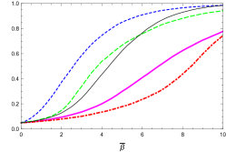
(a) $\bar{\kappa}=0$, $T=5$

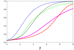
(b) $\bar{\kappa}=0$, $T=20$

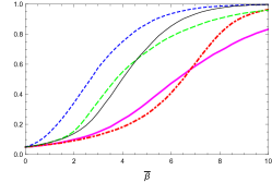
(c) $\bar{\kappa}=0$, $T=50$

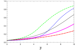
(d) $\bar{\kappa}=5$, $T=5$

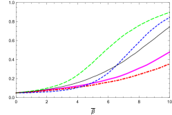
(e) $\bar{\kappa}=5$, $T=20$

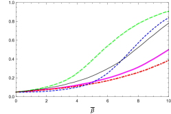
(f) $\bar{\kappa}=5$, $T=50$

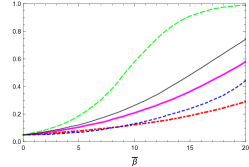
(g) $\bar{\kappa}=20$, $T=5$

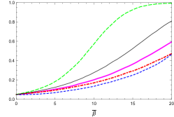
(h) $\bar{\kappa}=20$, $T=20$

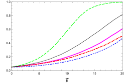
(i) $\bar{\kappa}=20$, $T=50$

Figure 1: Power for SB (continuous time)

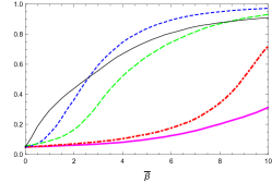
(a) $\bar{\kappa}=0$, $T=5$

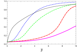
(b) $\bar{\kappa}=0$, $T=20$

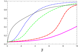
(c) $\bar{\kappa}=0$, $T=50$

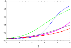
(d) $\bar{\kappa}=5$, $T=5$

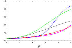
(e) $\bar{\kappa}=5$, $T=20$

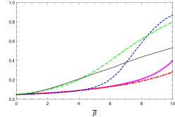
(f) $\bar{\kappa}=5$, $T=50$

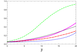
(g) $\bar{\kappa}=20$, $T=5$

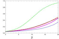
(h) $\bar{\kappa}=20$, $T=20$

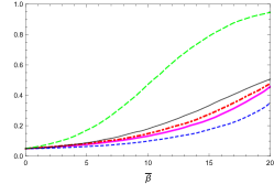
(i) $\bar{\kappa}=20$, $T=50$

Figure 2: Power for GBM (continuous time)

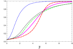
(a) $\bar{\kappa}=0$, $T=5$

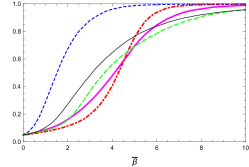
(b) $\bar{\kappa}=0$, $T=20$

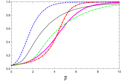
(c) $\bar{\kappa}=0$, $T=50$

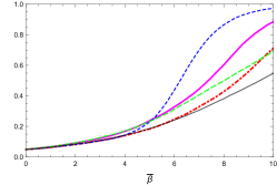
(d) $\bar{\kappa}=5$, $T=5$

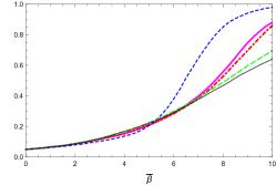
(e) $\bar{\kappa}=5$, $T=20$

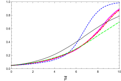
(f) $\bar{\kappa}=5$, $T=50$

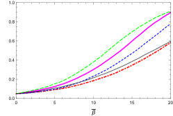
(g) $\bar{\kappa}=20$, $T=5$

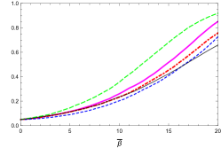
(h) $\bar{\kappa}=20$, $T=20$

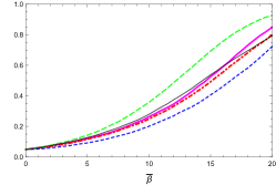
(i) $\bar{\kappa}=20$, $T=50$

Figure 3: Power for RS (continuous time)

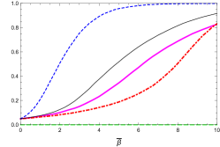
(a) $\bar{\kappa}=0$, $T=60$

(b) $\bar{\kappa}=0$, $T=240$

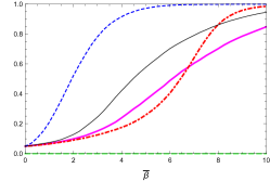
(c) $\bar{\kappa}=0$, $T=600$

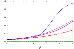
(d) $\bar{\kappa}=5$, $T=60$

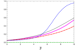
(e) $\bar{\kappa}=5$, $T=240$

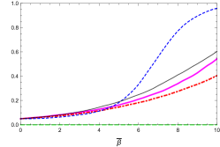
(f) $\bar{\kappa}=5$, $T=600$

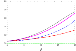
(g) $\bar{\kappa}=20$, $T=60$

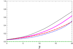
(h) $\bar{\kappa}=20$, $T=240$

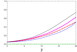
(i) $\bar{\kappa}=20$, $T=600$

Figure 4: Power for SB (discrete time)

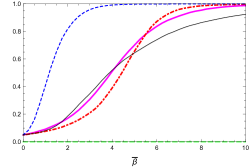
(a) $\bar{\kappa}=0$, $T=60$

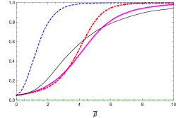
(b) $\bar{\kappa}=0$, $T=240$

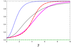
(c) $\bar{\kappa}=0$, $T=600$

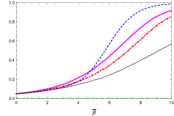
(d) $\bar{\kappa}=5$, $T=60$

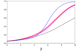
(e) $\bar{\kappa}=5$, $T=240$

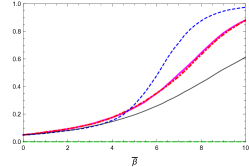
(f) $\bar{\kappa}=5$, $T=600$

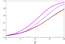
(g) $\bar{\kappa}=20$, $T=60$

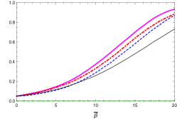
(h) $\bar{\kappa}=20$, $T=240$

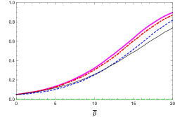
(i) $\bar{\kappa}=20$, $T=600$

Figure 5: Power for GARCH with $\alpha=0.9$ and $\theta=0.1$ (discrete time)

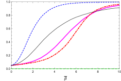
(a) $\bar{\kappa}=0$, $T=60$

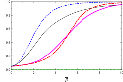
(b) $\bar{\kappa}=0$, $T=240$

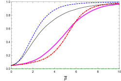
(c) $\bar{\kappa}=0$, $T=600$

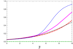
(d) $\bar{\kappa}=5$, $T=60$

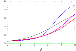
(e) $\bar{\kappa}=5$, $T=240$

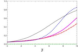
(f) $\bar{\kappa}=5$, $T=600$

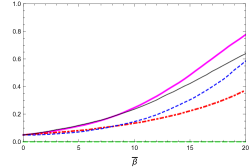
(g) $\bar{\kappa}=20$, $T=60$

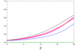
(h) $\bar{\kappa}=20$, $T=240$

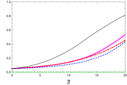
(i) $\bar{\kappa}=20$, $T=600$

Figure 6: Power for GARCH with $\alpha=0.1$ and $\theta=0.9$ (discrete time)

Figures 1-6 present the results on finite sample power properties of the tests considered. In our simulations, we consider the DGPs in (12) in continuous time and (14) in discrete time with $\bar{\beta}$ ranging from 0 to 20. All the power curves presented in the figures are size-adjusted. Taking into account the results of finite sample size performance of the tests and their comparisons, we mainly focus on two tests: the Cauchy RT and our test, in the analysis of finite sample power properties. For comparison, the analysis also provides the numerical results on the finite sample power of the OLS, BQ and RLRT tests.

In Figure 1 for the case of the structural break in volatility, one observes that the Cauchy RT test appears to be superior to other testing approaches (except in the cases with $\bar{\kappa}=0$ and large $\bar{\beta}$). At the same time, the proposed test $\tau(\hat{\sigma})$ also appears to have good finite sample power properties especially in the case of highly persistent predictors.

Figure 2 provides the numerical results on finite sample properties of the tests in the geometric Brownian motion case. For the case of a unit root regressor, the power properties of the proposed test based on $\tau(\hat{\sigma})$ appear to outperform those of the Cauchy RT test which in turn outperforms other tests considered. However, the finite sample power performance of the Cauchy RT test improves in the case of near unit root regressor with $\bar{\kappa}=5$ and $\bar{\kappa}=20$.

The power curves for the regime switching case presented in Figure 3 demonstrate that the test based on the proposed test $\tau(\hat{\sigma})$ has better power properties than other tests in the case $\bar{\kappa}=0.$ For the case of the near unit root persistence in the regressor, the power properties of the Cauchy RT test appear to be better than those of the test based on $\tau(\hat{\sigma})$ for relatively small sample sizes (small values of $T$). However, as the sample size increases, the test based on $\tau(\hat{\sigma})$ becomes more powerful than the Cauchy RT test (see, e.g., Figure 3 for the case $\bar{\kappa}=5$ and $T=50$). For large deviations from a unit root regressor ($\bar{\kappa}=20$), the Cauchy RT is more powerful than other tests, but the power curves appear to be very similar.

Figures 4-6 present the numerical results on power properties under discrete time settings for all the tests considered except Cauchy RT which is inapplicable in discrete time settings. Results in the figures are provided for the cases of the structural break in volatility (Figure 4); the GARCH cases with $(\alpha,\theta)=(0.9,0.1)$ (Figure 5) and $(\alpha,\theta)=(0.1,0.9)$ (Figure 6). For all the cases, the conclusions on power properties of the tests and their comparisons are virtually the same as in the continuous time framework.

Overall, the numerical results on finite sample properties of the tests indicate good performance of the test based on $\tau(\hat{\sigma})$ in comparison to the Cauchy RT. Again, the latter test is inapplicable in the discrete time settings. Their relative finite sample performances vary across different models. Which test should be used in practice depends on the availability of high frequency data as well as the size-power trade-off for a specific model. Therefore, the test proposed in this paper and the Cauchy RT complement rather than substitute one another.

6 Conclusion

Endogenously persistent regressors have been extensively analyzed in the predictive regression literature. A widely believed characteristic of stock returns is heteroskedastic and persistent volatility, which is often ignored in the predictive regression literature except for Choi et al. (2016). These two characteristics cause standard hypothesis tests to become substantially biased and often over-reject the null of no predictability. The main contribution of this paper is to provide an inference method that is designed to be robust to these problematic characteristics of predictive regression data. The proposed method relies on the Cauchy estimator and a kernel-based nonparametric correction of volatility. Its theoretical validity is provided by analyzing the asymptotic size and power properties. Moreover, it is shown through a simulation study that the proposed method has a reliable finite sample performance compared to the most advanced existing inference methods.

Our inference method is comparable to the method proposed by Choi et al. (2016). Similar to our method, their approach relies on the Cauchy estimator and a nonparametric volatility correction. However, their approach to the volatility correction is quite different from ours, and its applicability is limited to a predictive regression equipped with appropriate high frequency data. In terms of finite sample properties, our method and the method by Choi et al. (2016) perform well and have good size and power performances under continuous time settings. However, unlike our method, Choi et al. (2016) method is not applicable under discrete time settings. In contrast, our method can be applied to a discrete time model as well as a discrete sample collected from an underlying continuous time model. Therefore, our method is more flexible and widely applicable since it can be applied to both high and low frequency data.

A further approach to robust inference in predictive regressions under heterogeneous and persistent volatility as well as endogenous, persistent or heavy-tailed regressors is provided by the simple to implement robust $t$-statistic inference approach (see Ibragimov and Müller (2010)) based on asymptotically normal group Cauchy estimators of a regression parameter of interest. This approach will be explored in a companion paper now in preparation.

Online Supplementary Material

Ibragimov, R., Kim, J, and Skrobotov, A. (2022): Supplement to ‘‘New robust inference for predictive regressions,’’ Econometric Theory Supplementary Material. To view, please visit:

Table 1: Size for the continuous time models

		$\bar{\kappa}=0$			$\bar{\kappa}=5$			$\bar{\kappa}=20$
T		5	20	50	5	20	50	5	20	50
CNST	OLS	42.2	42.0	43.0	19.5	19.5	19.7	11.1	11.2	10.9
	BQ	8.6	4.9	4.3	7.5	4.5	4.2	8.6	4.1	3.2
	RLRT	8.5	7.7	8.1	5.4	5.9	5.6	4.8	5.2	5.3
	Cauchy RT	5.3	4.9	5.3	5.2	5.4	4.7	5.5	5.1	5.1
	$\tau(\hat{\sigma})$	5.6	5.0	5.3	5.4	5.0	5.1	5.4	5.0	4.8
SB	OLS	38.3	38.8	39.9	29.6	30.8	31.2	24.3	26.4	26.0
	BQ	18.1	12.9	11.9	17.0	15.1	14.1	17.4	14.8	14.3
	RLRT	23.8	22.8	23.6	21.0	21.9	21.8	22.4	24.5	23.6
	Cauchy RT	5.6	5.0	5.1	5.2	5.3	5.0	5.4	5.0	4.9
	$\tau(\hat{\sigma})$	8.0	6.7	6.3	7.8	6.5	6.0	7.9	6.4	6.0
RS	OLS	42.9	43.6	44.6	22.0	23.4	24.5	14.9	18.9	19.5
	BQ	8.8	6.3	6.0	9.8	7.2	6.8	12.6	8.9	8.4
	RLRT	9.3	10.0	10.7	7.5	9.4	9.6	9.6	13.0	14.2
	Cauchy RT	5.0	4.8	5.2	4.9	4.9	4.9	5.4	5.1	4.8
	$\tau(\hat{\sigma})$	5.2	5.4	6.1	5.2	5.1	5.8	5.6	5.8	5.8
GBM	OLS	52.2	53.7	53.1	28.6	30.2	30.9	23.2	26.0	27.0
	BQ	16.8	12.5	11.3	13.9	12.4	13.2	15.8	11.7	12.0
	RLRT	21.7	22.3	21.9	16.3	17.8	19.0	21.4	23.3	23.5
	Cauchy RT	4.4	4.7	4.4	4.3	4.5	4.4	4.6	4.5	4.5
	$\tau(\hat{\sigma})$	5.4	5.5	6.1	5.7	5.7	5.9	5.7	5.9	6.5

The parameter $\bar{\kappa}$ measures the degree of persistence in the predictor. The sample size corresponds to $T$ yearly observations (total $12T$ observations). CNST, SB, GBM, and RS denote respectively constant volatility, structural break, geometric Brownian motion, and regime switching in volatility.

Table 2: Size for the discrete time models with CNST and SB

		$\bar{\kappa}=0$			$\bar{\kappa}=5$			$\bar{\kappa}=20$
T		5	20	50	5	20	50	5	20	50
CNST	OLS	43.9	43.8	44.7	19.4	19.8	20.1	9.7	11.2	10.8
	BQ	8.4	5.2	4.8	7.8	4.9	4.5	9.2	4.1	3.4
	RLRT	8.3	8.0	8.1	5.2	5.4	5.3	4.1	5.4	5.3
	$\tau(\hat{\sigma})$	5.5	5.1	5.0	5.5	4.8	5.1	5.1	5.2	5.2
SB	OLS	38.0	39.6	40.0	29.1	31.1	31.4	22.1	26.1	26.8
	BQ	17.2	12.8	12.3	16.5	15.1	14.5	17.7	15.0	15.2
	RLRT	23.1	23.5	24.2	19.9	21.8	21.4	21.2	24.6	25.1
	$\tau(\hat{\sigma})$	8.0	6.7	6.3	7.9	6.2	5.8	7.5	6.5	6.2
ARCH(1)	OLS	45.0	44.1	43.5	23.5	22.5	21.2	17.2	17.0	15.2
$\alpha=0.5773$	BQ	9.7	5.4	4.8	9.5	5.8	4.6	13.1	6.3	4.6
$\xi=4$	RLRT	9.6	8.8	8.7	9.0	7.9	6.7	13.1	11.3	9.1
	$\tau(\hat{\sigma})$	6.1	5.4	6.0	6.1	5.2	5.4	6.0	5.9	6.1
ARCH(1)	OLS	45.8	44.0	43.6	24.4	24.1	22.6	19.7	19.8	18.1
$\alpha=0.7325$	BQ	10.2	6.2	5.2	10.4	7.1	5.8	14.7	8.3	6.8
$\xi=3$	RLRT	10.7	10.0	9.2	10.6	10.0	8.1	15.9	14.9	12.9
	$\tau(\hat{\sigma})$	5.9	5.8	6.5	6.2	5.6	6.0	6.4	6.1	6.1
IGARCH(1,1)	OLS	44.9	45.8	45.6	20.1	21.8	24.3	11.1	14.9	17.3
$\alpha=0.9$	BQ	8.9	5.8	6.0	7.8	6.0	6.9	9.3	5.3	6.4
$\beta=0.1$	RLRT	9.1	10.1	11.5	5.7	8.3	9.8	6.2	9.0	11.5
	$\tau(\hat{\sigma})$	6.2	5.5	5.5	5.8	5.6	6.0	5.9	5.8	5.7
IGARCH(1,1)	OLS	46.0	46.5	45.1	26.9	28.5	28.0	21.6	26.1	26.2
$\alpha=0.1$	BQ	11.7	8.3	8.1	12.7	10.4	10.9	16.4	12.2	13.4
$\beta=0.9$	RLRT	13.3	13.0	12.7	13.7	14.7	15.1	20.2	23.7	23.2
	$\tau(\hat{\sigma})$	6.3	6.4	7.4	6.9	6.7	7.2	6.6	6.9	6.9

The parameter $\bar{\kappa}$ measures the degree of persistence in the predictor. The sample size corresponds to $T$ yearly observations (total $12T$ observations). CNST, SB, GBM, and RS denote respectively constant volatility, structural break, geometric Brownian motion, and regime switching in volatility.

OLS:   , Bonf. Q:${\color[rgb]{1,0,0}\rule[2.0pt]{4.80005pt}{1.7pt}\ \mathbf{\cdot}\ \rule[2.0pt]{4.80005pt}{1.7pt}\ }$ RLRT:      , Cauchy RT:      , NP: 

OLS:   , Bonf. Q:${\color[rgb]{1,0,0}\rule[2.0pt]{4.80005pt}{1.7pt}\ \mathbf{\cdot}\ \rule[2.0pt]{4.80005pt}{1.7pt}\ }$ RLRT:      , Cauchy RT:      , NP: 

OLS:   , Bonf. Q:${\color[rgb]{1,0,0}\rule[2.0pt]{4.80005pt}{1.7pt}\ \mathbf{\cdot}\ \rule[2.0pt]{4.80005pt}{1.7pt}\ }$ RLRT:      , Cauchy RT:      , NP: 

OLS:   , Bonf. Q:${\color[rgb]{1,0,0}\rule[2.0pt]{4.80005pt}{1.7pt}\ \mathbf{\cdot}\ \rule[2.0pt]{4.80005pt}{1.7pt}\ }$ RLRT:      , NP: 

OLS:   , Bonf. Q:${\color[rgb]{1,0,0}\rule[2.0pt]{4.80005pt}{1.7pt}\ \mathbf{\cdot}\ \rule[2.0pt]{4.80005pt}{1.7pt}\ }$ RLRT:      , NP: 

OLS:   , Bonf. Q:${\color[rgb]{1,0,0}\rule[2.0pt]{4.80005pt}{1.7pt}\ \mathbf{\cdot}\ \rule[2.0pt]{4.80005pt}{1.7pt}\ }$ RLRT:      , NP: 

This supplement includes four appendices, Appendices A, B, C, and D. In Appendix A, we consider a class of nonlinear IV estimators, and discuss why the Cauchy estimator, which is a special case of nonlinear IV estimators, is useful in inference problems. Appendix B presents some useful lemmas, Lemmas S.1-S.8, and their proofs; Appendix C provides the proofs of the main results in the paper; and Appendix D provides some additional simulation results on finite sample performance of inference approaches dealt with.

Appendix A: Nonlinear IV Approaches

As mentioned in the main paper, the Cauchy estimator $\check{\beta}$ is the special case of a class of nonlinear IV estimators $\tilde{\beta}(\gamma)$ with $\gamma(\cdot)=sign(\cdot)$, where

$$\tilde{\beta}(\gamma)=\left(\sum_{t=1}^{T}\gamma(x_{t-1})x_{t-1}\right)^{-1}\sum_{t=1}^{T}\gamma(x_{t-1})y_{t}$$

for some function $\gamma:\mathbb{R}\to\mathbb{R}$. Clearly, $\tilde{\beta}(sign)=\check{\beta}$. Moreover, if we let $\iota$ be an identity function: $\iota(x)=x$, then $\tilde{\beta}(\iota)$ becomes the OLS estimator $\hat{\beta}$. In this section, we discuss why the choice of $\gamma(\cdot)=sign(\cdot)$, as in the Cauchy estimator, is important and useful when considering the class of nonlinear IV estimators in an inference problem. To explain the idea, we focus on the issues about the predictor $x_{t}$, and assume that $v_{t}=\sigma$ for all $t\geq 1$.

A.1 Nonstationary Predictor

The asymptotics for (near) unit root processes under various transformations are well known (see Park and Phillips (2001) and Park (2003)). For instance, let $x_{t}$ be a unit root process and $(x_{t},\sum_{s=1}^{t}\varepsilon_{s})$ satisfy the functional CLT with a limiting bivariate Brownian motion $(X,W)$. It then follows from Park and Phillips (2001) that for regularly integrable functions $f$ and $g^{2}$

$$\frac{1}{T^{1/2}}\sum_{t=1}^{T}f(x_{t-1}) \to_{d}L_{X}(1,0)\int_{-\infty}^{\infty}f(x)dx,$$ (S.1)

$$\frac{1}{T^{1/4}}\sum_{t=1}^{T}g(x_{t-1})\varepsilon_{t} \to_{d}\left(L_{X}(1,0)\int_{-\infty}^{\infty}g^{2}(x)dx\right)^{1/2}Z(1),$$

where $L_{X}(1,0)$ is the local time at the origin of $X$ and $Z$ is a Brownian motion independent of $X$. In particular, $\left(L_{X}(1,0)\int_{-\infty}^{\infty}g^{2}(x)dx\right)^{1/2}Z(1)=_{d}\mathbb{MN}\left(0,L_{X}(1,0)\int_{-\infty}^{\infty}g^{2}(x)dx\right)$, where $\mathbb{MN}$ is a mixed normal distribution.

On the other hand, if $f$ and $g^{2}$ are asymptotically homogeneous functions, then

$$\frac{1}{T}f_{\nu}(T^{1/2})\sum_{t=1}^{T}f(x_{t-1}) \to_{d}\int_{0}^{1}f_{H}(X(r))dr,$$ (S.2)

$$\frac{1}{T^{1/2}g_{\nu}(T^{1/2})}\sum_{t=1}^{T}g(x_{t-1})\varepsilon_{t} \to_{d}\int_{0}^{1}g_{H}(X(r))dW(r),$$

where $F_{\nu}$ and $F_{H}$ are, respectively, the asymptotic order and the limit homogeneous function of asymptotically homogeneous function $F=f,g$. The reader is referred to Section 3 of Park and Phillips (2001) for more detailed discussions about the asymptotics (S.1) and (S.2) as well as the precise definitions of the regularly integrable and asymptotically homogeneous functions. Note also that for a near unit root process the asymptotics (S.1) and (S.2) remain valid if $X$ is replaced by the limiting Ornstein-Uhlenbeck process of $(x_{t})$ (see, e.g., Section 3 of Park (2003)).

Importantly, the limit distribution of $\sum_{t=1}^{T}g(x_{t-1})\varepsilon_{t}$ in (S.2) is not Gaussian for an asymptotically homogeneous $g^{2}$ except in some special cases including $g_{H}(x)=sign(x)$. In particular, the sign function $sign(\cdot)$ is asymptotically homogeneous with $sign_{\nu}(\lambda)=1$ for all $\lambda$ and $sign_{H}(x)=sign(x)$. Since $\int_{0}^{r}sign(X(s))dW(s)$ is a Brownian motion by Lévy’s characterization of Brownian motion, we have

$$\frac{1}{T^{1/2}}\sum_{t=1}^{T}sign(x_{t-1})\varepsilon_{t}\to_{d}W(1).$$

Using the asymptotics (S.1) and (S.2), one may construct a nonlinear IV estimator $\tilde{\beta}(\gamma)$ being asymptotically Gaussian for a proper choice of $\gamma$, i.e., for $\gamma$ square integrable or the sign function. For such $\gamma$, one may use the following test statistic

$$\tilde{\tau}(\gamma)=\frac{\sum_{t=1}^{T}\gamma(x_{t-1})x_{t-1}}{\left(\sum_{t=1}^{T}\gamma^{2}(x_{t-1})\right)^{1/2}}\times\tilde{\beta}(\gamma)$$

to test the null hypothesis of $\beta=0$.

Proposition S.1.

Let Assumption 2.1 hold with $v_{t}=\sigma$ for all $t\geq 1$, and let $(x_{t})$ be a unit root process. Further assume that the convergences in (S.1) and (S.2) hold.

(a) Let $\gamma(\cdot)=sign(\cdot)$ or $\gamma^{2}$ be regularly integrable. Under $\beta=0$,

$$\tilde{\tau}(\gamma)\to_{d}\mathbb{N}(0,\sigma^{2})$$

(b) Let $\gamma(\cdot)=sign(\cdot)$. Under $\beta\neq 0$,

$$\frac{1}{T}\tilde{\tau}(\gamma)\to_{d}\beta\int_{0}^{1}|B(r)|dr.$$

(c) Let $\gamma^{2}(x)$ be regularly integrable, and let $x\gamma(x)$ be either asymptotically homogeneous or regularly integrable such that $\int_{-\infty}^{\infty}x\gamma(x)dx\neq 0$. Under $\beta\neq 0$, we have $\tilde{\tau}(\gamma)\to_{p}\infty$ and $\tilde{\tau}(\gamma)=o_{p}(T)$.

Proof.

Note that

$$\tilde{\tau}(\gamma)=\frac{\sum_{t=1}^{T}\gamma(x_{t-1})y_{t}}{\left(\sum_{t=1}^{T}\gamma^{2}(x_{t-1})\right)^{1/2}}=\beta\frac{\sum_{t=1}^{T}\gamma(x_{t-1})x_{t-1}}{\left(\sum_{t=1}^{T}\gamma^{2}(x_{t-1})\right)^{1/2}}+\frac{\sum_{t=1}^{T}\gamma(x_{t-1})u_{t}}{\left(\sum_{t=1}^{T}\gamma^{2}(x_{t-1})\right)^{1/2}}.$$

The stated results in the parts (a) and (b) then follow immediately from the convergences (S.1) and (S.2) since, in particular for $\gamma(\cdot)=sign(\cdot)$, we have

$$\sum_{t=1}^{T}sign^{2}(x_{t-1})=T(1+o_{p}(1)),\quad\frac{1}{T^{3/2}}\sum_{t=1}^{T}|x_{t-1}|\to_{d}\int_{0}^{1}|B_{r}|dr.$$

We let $\iota(x)=x$. As for Part (c), we first let $\gamma^{2}$ and $\iota\gamma$ be regularly integrable. Then, under $\beta\neq 0$,

$$\tilde{\tau}(\gamma)=\beta\frac{\sum_{t=1}^{T}\gamma(x_{t-1})x_{t-1}}{\left(\sum_{t=1}^{T}\gamma^{2}(x_{t-1})\right)^{1/2}}(1+o_{p}(1))$$

and

$$\frac{1}{T^{1/4}}\frac{\sum_{t=1}^{T}\gamma(x_{t-1})x_{t-1}}{\left(\sum_{t=1}^{T}\gamma^{2}(x_{t-1})\right)^{1/2}}\to_{d}\frac{L_{X}(1,0)\int_{-\infty}^{\infty}\gamma(x)xdx}{\left(L_{X}(1,0)\int_{-\infty}^{\infty}\gamma^{2}(x)dx\right)^{1/2}}$$

by (S.1), from which $\tilde{\tau}(\gamma)=o_{p}(T)$.

On the other hand, if $\iota\gamma$ is asymptotically homogeneous and $\gamma^{2}$ is regularly integrable, then

$$\frac{1}{T^{3/4}(\iota\gamma)_{\nu}(T^{1/2})}\frac{\sum_{t=1}^{T}\gamma(x_{t-1})x_{t-1}}{\left(\sum_{t=1}^{T}\gamma^{2}(x_{t-1})\right)^{1/2}}\to_{d}\frac{\int_{0}^{1}(\iota\gamma)_{H}(X_{r})dr}{\left(L_{X}(1,0)\int_{-\infty}^{\infty}\gamma^{2}(x)dx\right)^{1/2}}$$

by (S.1) and (S.2). Since $\gamma^{2}$ is regularly integrable, $\gamma(\lambda)\lambda^{1/2}=o(1)$, and hence, $(\iota\gamma)(\lambda)=o(\lambda^{1/2})$. It then follows from the construction of the asymptotically homogeneous function that $(\iota\gamma)_{\nu}(T^{1/2})=o(T^{1/4})$. Therefore, if $\gamma^{2}$ is regularly integrable and $\iota\gamma$ is either regularly integrable or asymptotically homogeneous, then $\tilde{\tau}(\gamma)=o_{p}(T)$ as required. ∎

According to Proposition S.1 (a) and (b), one may easily conduct a Gaussian inference using the nonlinear IV estimator with $\gamma(\cdot)=sign(\cdot)$. Moreover, Proposition S.1 (a) and (c) imply that a similar Gaussian inference can be conducted using a square integrable $\gamma$. However, Proposition S.1 (b) and (c) imply that under $\beta\neq 0$ the divergence rate of $\tilde{\tau}(sign)$ is faster than that of $\tilde{\tau}(\gamma)$ with a square integrable $\gamma$, which implies the test with $\tilde{\tau}(sign)$ tends to have a better power property than the test with $\tilde{\tau}(\gamma)$ in finite samples.

A.2 Stationary Predictor

For a stationary $x_{t}$, the asymptotic distribution of the nonlinear IV based test statistic $\tilde{\tau}(\gamma)$ can be obtained easily and is given by a Gaussian distribution under $\beta=0$ when $\mathbb{E}|\gamma^{2}(x_{t-1})|<\infty$. However, if $x_{t}$ has a heavy-tailed marginal distribution and $\mathbb{E}|\gamma^{2}(x_{t-1})|$ is unbounded for a given $\gamma$, then the limit distribution of $\tilde{\tau}(\gamma)$ is generally non-Gaussian. Therefore, the choice of $\gamma$, as in the unit root type predictor, is important in a Gaussian inference relying on the nonlinear IV. Importantly, the Cauchy based test statistic is always asymptotically Gaussian since $\mathbb{E}|\gamma^{2}(x_{t-1})|=1$, and hence, the result of Proposition S.1 (a) remains valid. Moreover, it is shown in Theorem 3.3 that the test statistic based on the Cauchy estimator diverges under the alternative hypothesis and its divergence rate is no slower than the usual $\sqrt{T}$ rate for any nontrivial stationary process. As a conclusion of Section 2.3, the Cauchy estimator can be used to construct a robust inference having a Gaussian limit with no significant loss of testing power compared with other nonlinear IV based methods.

Appendix B: Useful Lemmas

Lemma S.1.

Let Assumption 3.1 hold, and let $f_{h}(s)=f(s/h)$ for $f=K,K^{2}$. We have

$$\sup_{h\leq r\leq 1}\left|\frac{1}{hT}\sum_{t=1}^{T}f_{h}(r-t/T)-\int_{0}^{1}f(s)ds\right|=O(1/(h^{2}T)).$$

Proof.

We only prove the result for the case $f=K$ since the argument in the case $f=K^{2}$ is similar. For the proof, we define a function $I_{r,h}:[0,1]\to\{0,1\}$ for $r\in[0,1]$ and $h>0$ as $I_{r,h}(s)=1\{r-h\leq s\leq r\}$. We then write

$$\sup_{h\leq r\leq 1-h}\sum_{t=1}^{T}\int_{t-1}^{t}|K_{h}(r-t/T)-K_{h}(r-s/T)|ds=A_{T}(r)+B_{T}(r)+C_{T}(r),$$

where

$$A_{T}(r) =\sum_{t=1}^{T}\left(\int_{t-1}^{t}|K_{h}(r-t/T)-K_{h}(r-s/T)|ds\right)I_{r,h-1/T}(t/T),$$

$$B_{T}(r) =\sum_{t=1}^{T}\left(\int_{t-1}^{t}|K_{h}(r-t/T)-K_{h}(r-s/T)|ds\right)(1-I_{r,h+1/T}(t/T)),$$

$$C_{T}(r) =\sum_{t=1}^{T}\left(\int_{t-1}^{t}|K_{h}(r-t/T)-K_{h}(r-s/T)|ds\right)(I_{r,h+1/T}(t/T)-I_{r,h-1/T}(t/T)).$$

By Assumption 3.1 (a) and (c), we have

$$\sup_{h\leq r\leq 1}A_{T}(r)\leq C\sum_{t=1}^{T}\int_{t-1}^{t}\frac{|t-s|}{hT}ds\leq C\frac{1}{h}.$$

Moreover, $\int_{t-1}^{t}|K_{h}(r-t/T)-K_{h}(r-s/T)=0$ for all $t$ satisfying $I_{r,h+1/T}(t/T)=0$ by Assumption 3.1 (a), and hence, $\sup_{h\leq r\leq 1}B_{T}(r)=0$. Moreover, it may be deduced from Assumption 3.1 (a) that

$$\sup_{h\leq r\leq 1}\sum_{t=1}^{T}|I_{r,h+1/T}(t/T)-I_{r,h-1/T}(t/T)|\leq 2,$$

from which, jointly with Assumption 3.1 (b), we have $\sup_{h\leq r\leq 1}C_{T}(r)=O(1)$. The stated result for $f=K$ then follows immediately since

$$\frac{1}{hT}\int_{0}^{T}K_{h}(r-s/T)ds=\frac{1}{h}\int_{0}^{1}K_{h}(r-s)ds=\int_{0}^{1}K(s)ds$$ (S.3)

for $r\in[h,1]$, by Assumption 3.1 (a) and the change of variable in integrals. ∎

Lemma S.2.

Let Assumption 2.2 hold. As $h\to 0$,

$$\sup_{r\in\mathcal{C}_{h},0<h^{\prime}<h}|\sigma_{T}^{2}(r)-\sigma_{T}^{2}(r-h^{\prime})|=o_{a.s.}(1).$$

Proof.

We have

$$|\sigma_{T}^{2}(r)-\sigma_{T}^{2}(r-h^{\prime})|\leq|\sigma_{T}^{2}(r)-\sigma^{2}(r)|+|\sigma_{T}^{2}(r-h^{\prime})-\sigma^{2}(r-h^{\prime})|+|\sigma^{2}(r)-\sigma^{2}(r-h^{\prime})|.$$

Note that, under our conventions, $\sup_{0\leq r\leq 1}|\sigma_{T}^{2}(r)-\sigma^{2}(r)|=o_{a.s.}(1)$ since $\sigma_{T}\to_{d}\sigma$ in Assumption 2.2 holds almost surely on $\mathbf{D}_{\mathbb{R}^{+}}[0,1]$ endowed with the uniform topology. It follows that the first two terms are of $o_{a.s.}(1)$.

As for the last term, we note that a càdlàg function is uniformly right-continuous on finite closed intervals (see, e.g., Applebaum (2009), pp. 140). It follows that an associated càdlàg function $\sigma_{-}(r)=\sigma(r-)$ is uniformly left continuous, and hence,

$$\sup_{r\in[h,1],0<h^{\prime}<h}|\sigma^{2}(r-)-\sigma^{2}(r-h^{\prime})|=o_{a.s.}(1).$$

However, $\sigma^{2}(r-)=\sigma^{2}(r)$ for all $r\in\mathcal{C}_{h}$, which completes the proof. ∎

Lemma S.3.

Let Assumptions 2.2 and 3.1 hold. If $h\to 0$ and $h^{2}T\to\infty$, then for any fixed real number $c\geq 0$

$$\sup_{r\in\mathcal{C}_{h}}|\hat{\sigma}_{1}^{2}(r-c/T)-\sigma_{T}^{2}(r)|=o_{p}(1).$$

Proof.

We have

$$\hat{\sigma}_{1}^{2}(r-c/T)-\sigma_{T}^{2}(r)=\frac{\sum_{t=1}^{T}\left(\sigma_{T}^{2}(t/T)-\sigma_{T}^{2}(r)\right)K_{h}(r-c/T-t/T)}{\sum_{t=1}^{T}K_{h}(r-c/T-t/T)}$$

and $\sup_{h\leq r\leq 1}hT/(\sum_{t=1}^{T}K_{h}(r-c/T-t/T))=O_{p}(1)$ by Lemma S.1 and Assumption 3.1 (a).

To complete the proof, we write

$$\frac{1}{hT}\sum_{t=1}^{T}\left(\sigma_{T}^{2}(t/T)-\sigma_{T}^{2}(r)\right)K_{h}(r-c/T-t/T)=A_{T}(r)+B_{T}(r),$$

where

$$A_{T}(r) =\frac{1}{hT}\sum_{t=1}^{T}\left(\sigma_{T}^{2}(t/T)1\{t/T\in(r-h,r]\}-\sigma_{T}^{2}(r)\right)K_{h}(r-c/T-t/T)ds,$$

$$B_{T}(r) =\frac{1}{hT}\sum_{t=1}^{T}\sigma_{T}^{2}(t/T)\left(1\{(t+c)/T\in[r-h,r]\}-1\{t/T\in(r-h,r]\}\right)K_{h}(r-c/T-t/T)ds.$$

We can deduce from Lemmas S.1 and S.2 that

$$\sup_{r\in\mathcal{C}_{h}}|A_{T}(r)|=\sup_{r\in\mathcal{C}_{h},0<h^{\prime}<h}|\sigma_{T}^{2}(r)-\sigma_{T}^{2}(r-h^{\prime})|\left(\frac{1}{hT}\sum_{t=1}^{T}K_{h}(r-t/T)\right)=o_{p}(1).$$

We note that $\sigma_{T}$ and $K$ are bounded due to Assumptions 2.1 (a) and 3.1 (b). Also, we have for a fixed $c\geq 0$ and large $T$

$$\left|1\left\{\frac{t+c}{T}\in[r-h,r]\right\}-1\left\{\frac{t}{T}\in(r-h,r]\right\}\right|$$

$$\leq 1\left\{\frac{t}{T}\in\left[r-\frac{c}{T}-h,r-h\right]\right\}+1\left\{\frac{t}{T}\in\left[r-\frac{c}{T},r\right]\right\},$$

and hence,

$$\sup_{h\leq r\leq 1}\sum_{t=1}^{T}\left|1\{(t+c)/T\in[r-h,r]\}-1\{t/T\in(r-h,r]\}\right|\leq 2c+2.$$

It follows that

$$\sup_{h\leq r\leq 1}|B_{T}(r)| \leq\frac{1}{hT}\sup_{h\leq r\leq 1}|\sigma_{T}^{2}(r)K(r)|\sup_{h\leq r\leq 1}\sum_{t=1}^{T}\left|1\{(t+c)/T\in[r-h,r]\}-1\{t/T\in(r-h,r]\}\right|$$

$$=O_{p}(1/(hT)).$$

This completes the proof. ∎

Lemma S.4.

Let Assumptions 2.1, 3.1 and 3.3 hold. If $h\to 0$, $h^{2}T\to\infty$ and $h^{\kappa}T=O(1)$ for some $\kappa>2$, then

$$\sup_{h\leq r\leq 1}|\hat{\sigma}_{2}^{2}(r)| =O_{p}\left(\left(\log(hT)/(hT)\right)^{1/2}T^{2q}\right).$$

Proof.

Since $\sup_{h\leq r\leq 1}hT/(\sum_{t=1}^{T}K_{h}(r-t/T))=O_{p}(1)$, it suffices to show that

$$\sup_{h\leq r\leq 1}\left|\sum_{t=1}^{T}v_{t}^{2}(\varepsilon_{t}^{2}-1)K_{h}(r-t/T)\right|=O_{p}((hT\log(hT))^{1/2}T^{2q}).$$

To complete the proof, we split the interval $[h,1]$ into $\bar{k}$ intervals of the form $I_{k}=1\{r|r_{k}\leq r\leq r_{k+1}\}$, where $r_{k}=h+kh^{\bar{\kappa}}$ for $k=0,\cdots,[(1-h)/h^{\bar{\kappa}}]$ for some $\bar{\kappa}\geq(\kappa+2)/2$. Then we can write

$$\sup_{h\leq r\leq 1}\left|\sum_{t=1}^{T}v_{t}^{2}(\varepsilon_{t}^{2}-1)K_{h}(r-t/T)\right| \leq\max_{0\leq k\leq\bar{k}}|S_{T}(r_{k})|+R_{T},$$

where $S_{t}(r_{k})=\sum_{s=1}^{t}v_{s}^{2}(\varepsilon_{s}^{2}-1)K_{h}(r_{k}-s/T)$ for $t=1,\cdots,T$, and

$$R_{T}=\max_{0\leq k\leq\bar{k}}\sup_{r\in I_{k}}\sum_{t=1}^{T}|v_{t}^{2}(\varepsilon_{t}^{2}-1)|\left|K_{h}(r-t/T)-K_{h}(r_{k}-t/T)\right|.$$

For $R_{T}$, we note that for each $k$, $r_{k+1}=r_{k}+h^{\bar{\kappa}}$ and

$$\left|K_{h}(r-t/T)-K_{h}(r_{k}-t/T)\right|=\left|K_{h}(r-t/T)-K_{h}(r_{k}-t/T)\right|1\{r_{k}-h\leq t/T\leq r_{k}+h^{\bar{\kappa}}\}$$

for $r\in I_{k}$. It follows that

$$R_{T} =\max_{0\leq k\leq\bar{k}}\sup_{r\in I_{k}}\sum_{t=1}^{T}|v_{t}^{2}(\varepsilon_{t}^{2}-1)|\left|K_{h}(r-t/T)-K_{h}(r_{k}-t/T)\right|1\{r_{k}-h\leq t/T\leq r_{k}+h^{\bar{\kappa}}\}$$

$$\leq Ch^{\bar{\kappa}-1}\sum_{t=1}^{T}|v_{t}^{2}(\varepsilon_{t}^{2}-1)|1\{r_{k}-h\leq t/T\leq r_{k}+h^{\bar{\kappa}}\}$$

$$\leq Ch^{\bar{\kappa}-1}\left(\max_{0\leq k\leq\bar{k}}\sum_{t=1}^{T}v_{t}^{4}1\{r_{k}-h\leq t/T\leq r_{k}+h^{\bar{\kappa}}\}\right)^{1/2}\left(\sum_{t=1}^{T}(\varepsilon_{t}^{2}-1)^{2}\right)^{1/2}$$

$$\leq O_{p}(h^{\bar{\kappa}-1}T^{1/2}(hT)^{1/2}),$$

where the second line follows from Assumption 3.1, the third line holds due to the Cauchy-Schwarz inequality, and the last line follows from the fact that for any $\bar{\kappa}\geq 1$

$$\max_{0\leq k\leq\bar{k}}\sum_{t=1}^{T}v_{t}^{4}1\{r_{k}-h\leq t/T\leq r_{k}+h^{\bar{\kappa}}\}\leq 2\sup_{h\leq r\leq 1}\sum_{t=1}^{T}v_{t}^{4}1\{r-h\leq t/T\leq r\}=O_{p}(hT).$$

Consequently, we have $R_{T}=O_{p}((hT)^{1/2})$ since $\bar{\kappa}\geq 2$ and $h^{2\bar{\kappa}-2}T\leq h^{\kappa}T=O(1)$.

As for $S_{T}(r_{k})$, we note that for each $k=1,\cdots,\bar{k}$, $(S_{t}(r_{k}),\mathcal{F}_{t})$ is a square integrable martingale since $(\varepsilon_{t}^{2}-1,\mathcal{F}_{t})$ is an MDS and $v_{t}^{2}$ is $\mathcal{F}_{t}$-adapted such that $\varepsilon_{t}^{2}-1$ has a finite second moment and $\sup_{r\in[h,1]}\sum_{t=1}^{T}v_{t}^{2}1\{r-h\leq t/T\leq r\}=O_{p}(hT)$ by Assumptions 2.1. The predictive quadratic variation $\langle S(r_{k})\rangle$ and the total quadratic variation $[S(r_{k})]$ of $S(r_{k})$ are respectively given by

$$\langle S(r_{k})\rangle_{T} =\sum_{t=1}^{T}v_{t}^{4}E[(\varepsilon_{t}^{2}-1)^{2}|\mathcal{F}_{t-1}]K_{h}^{2}(r_{k}-t/T),$$

$$[S(r_{k})]_{T} =\sum_{t=1}^{T}v_{t}^{4}(\varepsilon_{t}^{2}-1)^{2}K_{h}^{2}(r_{k}-t/T).$$

Clearly, $\max_{0\leq k\leq\bar{k}}\langle S(r_{k})\rangle_{T}=O_{p}(hT)$ and $\max_{0\leq k\leq\bar{k}}[S(r_{k})]_{T}=O_{p}(hTT^{4q})$. It follows that $\max_{0\leq k\leq\bar{k}}\left|\langle S(r_{k})\rangle_{T}+[S(r_{k})]_{T}\right|=O_{p}(hTT^{4q})$ which implies that for any $\delta$, we can find a constant $M>0$ such that

$$P\left(\max_{0\leq k\leq\bar{k}}\left|\langle S(r_{k})\rangle_{T}+[S(r_{k})]_{T}\right|<M(hTT^{4q})\right)\leq\delta.$$

Consequently, we have

$$P\left(\max_{0\leq k\leq\bar{k}}|S_{T}(r_{k})|>M(hTT^{4q}\log(hT))^{1/2}\right)$$

$$\leq P\left(\max_{0\leq k\leq\bar{k}}|S_{T}(r_{k})|>M(hTT^{4q}\log(hT))^{1/2},\max_{0\leq k\leq\bar{k}}\left|\langle S(r_{k})\rangle_{T}+[S(r_{k})]_{T}\right|<M(hTT^{4q})\right)+\delta$$

$$\leq\sum_{k=0}^{\bar{k}}P\left(|S_{T}(r_{k})|>M(hTT^{4q}\log(hT))^{1/2},\langle S(r_{k})\rangle_{T}+[S(r_{k})]_{T}<M(hTT^{4q})\right)+\delta$$

$$\leq\frac{2}{h^{\bar{\kappa}}}\exp\left(-M\log(hT)/2\right)+\delta,$$

where the last line follows from the two-sided martingale exponential inequality (see, e.g., Theorem 2.1 of Bercu and Touati (2008)). Moreover, $h^{-\bar{\kappa}}\exp\left(-M\log(hT)/2\right)=(h^{\bar{\kappa}}(hT)^{M/2})^{-1}\to 0$ for all $M\geq 2\bar{\kappa}$ as $h^{2}T\to\infty$. This completes the proof. ∎

Lemma S.5.

Let Assumptions 2.1, 3.1 and 3.2 hold. If $h\to 0$ and $h^{2}T\to\infty$, then

$$\sup_{h\leq r\leq 1}|\hat{\sigma}_{3}^{2}(r)|=O_{p}\left(T^{2p}/(hT)\right).$$

Proof.

By Lemma 3.1, we have $(\hat{\beta}-\beta)^{2}=O_{p}\left(T^{2p}\left(\sum_{t=1}^{T}x_{t-1}^{2}\right)^{-1}\right)$. Moreover, we may deduce from Lemma S.1 with Assumptions 3.1 that for some $0<M<\infty$

$$\sup_{h\leq r\leq 1}\left|\frac{\sum_{t=1}^{T}x_{t-1}^{2}K_{h}(r-t/T)}{\sum_{t=1}^{T}K_{h}(r-t/T)}\right|\leq\frac{M}{hT}\left(\sum_{t=1}^{T}x_{t-1}^{2}\right)(1+o_{p}(1)),$$

from which we have the stated result. ∎

Lemma S.6.

Let Assumptions 2.1, 3.1 and 3.2 hold. If $h\to 0$ and $h^{2}T\to\infty$, then

$$\sup_{h\leq r\leq 1}|\hat{\sigma}_{4}^{2}(r)|=O_{p}\left(T^{2p}/(hT)\right).$$

Proof.

As in the proof of Lemma S.5, we have $\sup_{h\leq r\leq 1}|\sum_{t=1}^{T}K_{h}(r-t/T)|^{-1}=O_{p}((hT)^{-1})$ and $\hat{\beta}-\beta=O_{p}\left(T^{p}\left(\sum_{t=1}^{T}x_{t-1}^{2}\right)^{-1/2}\right)$. Moreover, we have

$$\sup_{h\leq r\leq 1}\left|\sum_{t=1}^{T}x_{t-1}u_{t}K_{h}(r-t/T)\right|=O_{p}\left(T^{p}\left(\sum_{t=1}^{T}x_{t-1}^{2}\right)^{1/2}\right)$$

by Assumption 3.2. This completes the proof.

∎

Lemma S.7.

Let Assumptions 2.1, 3.1 and 3.2 hold. If $h\to 0$, $h^{2}T\to\infty$ and $h^{\kappa}T=O(1)$ for some $\kappa>2$, then

$$\sup_{h\leq r\leq 1}\frac{1}{\hat{\sigma}^{2}(r)},\quad\sup_{h\leq r\leq 1}\frac{1}{\hat{\sigma}_{1}^{2}(r)+\hat{\sigma}_{2}^{2}(r)}=O_{p}(1).$$

Proof.

It follows from Lemmas S.4-S.6 that

$$\frac{1}{\hat{\sigma}(r)}=\frac{\sum_{t=1}^{T}K_{h}(r-t/T)}{\sum_{t=1}^{T}\sigma_{T}^{2}(t/T)K_{h}(r-t/T)}+o_{p}(1)$$

uniformly in $r\in[h,1]$. However, $\sigma_{T}^{2}(r)\geq\underline{v}>0$ by Assumption 2.1, and hence, $\sup_{h\leq r\leq 1}1/\hat{\sigma}^{2}(r)\geq\underline{v}+o_{p}(1)=O_{p}(1)$. Similarly, we can show that $\sup_{h\leq r\leq 1}1/(\hat{\sigma}_{1}^{2}(r)+\hat{\sigma}_{2}^{2}(r))=O_{p}(1)$. ∎

Lemma S.8.

Under Assumptions 2.1 and 2.2,

$$\left(W_{T},\sigma_{T},\int\sigma_{T}(r)dW_{T}(r)\right)\to_{d}\left(W,\sigma,\int\sigma(r)dW(r)\right)$$

in $\mathbf{D}_{\mathbb{R}\times\mathbb{R}^{+}\times\mathbb{R}}[0,1]$.

Proof.

The lemma follows from Theorem 4.6 of Kurtz and Protter (1991) (see also Theorem 2.1 of Hansen (1992). ∎

Appendix C: Proofs of the Main Results

Proof of Lemmas 2.1.

The stated result follows immediately from Lemma S.8. ∎

Proof of Lemma 3.1.

The stated result follows immediately from Assumptions 2.1 and 3.2. ∎

Proof of Proposition 3.2.

Assumption 3.4 implies that $h^{2}T\to\infty$ and $h^{\kappa}T=O(1)$ for some $\kappa>2$. The stated results then follow immediately from Lemmas S.3-S.6. ∎

Proof of Theorem 3.3.

We define $\tilde{\sigma}$ by $\tilde{\sigma}(r)=\hat{\sigma}_{1}(r-1/T)+\hat{\sigma}_{2}(r-1/T)$ for $r\in[h,1]$ and $\tilde{\sigma}(r)=\sigma_{T}(r)$ for $r\in[0,h)$. We also define $\bar{\sigma}$ as

$$\bar{\sigma}(r)=\tilde{\sigma}(r)1\{\sigma(s)=\sigma(s-),s\in(r-h,r]\}+\sigma_{T}(r)1\{\sigma(s)\neq\sigma(s-),s\in(r-h,r]\}$$

for $r\in[h,1]$, and $\bar{\sigma}(r)=\sigma_{T}(r)$ for $r\in[0,h)$.

Clearly, $\bar{\sigma}(r)$ is a $\mathcal{F}_{Tr}$-adapted càdlàg process such that $\bar{\sigma}\to_{d}\sigma$ since

$$\sup_{0\leq r\leq 1}|\bar{\sigma}^{2}(r)-\sigma_{T}^{2}(r)|\leq\sup_{r\in\mathcal{C}_{h}}|\bar{\sigma}^{2}(r)-\sigma_{T}^{2}(r)|\leq\sup_{r\in\mathcal{C}_{h}}|\hat{\sigma}_{1}^{2}(r-1/T)-\sigma_{T}^{2}(r)|+\sup_{h\leq r\leq 1}|\hat{\sigma}_{2}(r)|$$

which is of $o_{p}(1)$ by Lemmas S.3 and S.4. It then follows from Lemma S.8 that under $\beta=0$

$$\tau(\bar{\sigma})=\frac{1}{\sqrt{T}}\sum_{t=1}^{T}\frac{sign(x_{t-1})y_{t}}{\bar{\sigma}(t/T)}=\frac{1}{\sqrt{T}}\sum_{t=1}^{T}sign(x_{t-1})\varepsilon_{t}\frac{\sigma_{T}(t/T)}{\bar{\sigma}(t/T)}\to_{d}\mathbb{N}(0,1).$$

To complete the proof, we show that

$$\tau(\hat{\sigma})-\tau(\tilde{\sigma}),\,\,\tau(\tilde{\sigma})-\tau(\bar{\sigma})=o_{p}(1).$$

We write

$$\tau(\hat{\sigma})-\tau(\tilde{\sigma})=A_{T}-B_{T}+C_{T},$$

where

$$A_{T} =\frac{1}{\sqrt{T}}\sum_{t=1}^{hT}sign(x_{t-1})\varepsilon_{t}\frac{\sigma_{T}(t/T)}{\hat{\sigma}((t-1)/T)},\quad B_{T}=\frac{1}{\sqrt{T}}\sum_{t=1}^{hT}sign(x_{t-1})\varepsilon_{t}\frac{\sigma_{T}(t/T)}{\tilde{\sigma}(t/T)},$$

$$C_{T} =\frac{1}{\sqrt{T}}\sum_{t=hT+1}^{T}sign(x_{t-1})\varepsilon_{t}\left(\frac{\sigma_{T}(t/T)}{\hat{\sigma}((t-1)/T)}-\frac{\sigma_{T}(t/T)}{\tilde{\sigma}(t/T)}\right).$$

To show $A_{T},B_{T}=o_{p}(1)$, we note that

$$\frac{1}{\sqrt{hT}}\sum_{t=1}^{hT}sign(x_{t-1})\varepsilon_{t}\sigma_{T}(t/T),\quad\frac{1}{\sqrt{hT}}\sum_{t=1}^{hT}sign(x_{t-1})\varepsilon_{t}=O_{p}(1)$$

by Lemma S.8. It follows that

$$A_{T} =\sqrt{h}\frac{1}{\hat{\sigma}(h)}\left(\frac{1}{\sqrt{hT}}\sum_{t=1}^{hT}sign(x_{t-1})\varepsilon_{t}\sigma_{T}(t/T)\right)=O_{p}(\sqrt{h})$$

since $1/\hat{\sigma}(h)=O_{p}(1)$ by Lemma S.7, and

$$B_{T} =\sqrt{h}\left(\frac{1}{\sqrt{hT}}\sum_{t=1}^{hT}sign(x_{t-1})\varepsilon_{t}\right)=O_{p}(\sqrt{h}).$$

For $C_{T}$, we have

$$|C_{T}| \leq\frac{1}{\sqrt{T}}\sum_{t=hT+1}^{T}|\sigma_{T}(t/T)\varepsilon_{t}|\left|\frac{\tilde{\sigma}^{2}(t/T)-\hat{\sigma}^{2}((t-1)/T)}{\hat{\sigma}((t-1)/T)\tilde{\sigma}(t/T)(\tilde{\sigma}(t/T)+\sigma_{T}(t/T))}\right|$$

$$\leq O_{p}(\sqrt{T})\times\sup_{h\leq r\leq 1}|\tilde{\sigma}^{2}(r)-\hat{\sigma}^{2}(r-1/T)|$$

since $\sum_{t=hT+1}^{T}|\sigma_{T}(t/T)\varepsilon_{t}|=O_{p}(T)$ and $1/\hat{\sigma}(r),1/\tilde{\sigma}(r)=O_{p}(1)$ uniformly in $h\leq r\leq 1$ by Lemma S.7. However, it follows from Lemmas S.5 and S.6 that

$$\sup_{h\leq r\leq 1}|\tilde{\sigma}^{2}(r)-\hat{\sigma}^{2}(r-1/T)|\leq\sup_{h\leq r\leq 1}|\hat{\sigma}_{3}^{2}(r)|+\sup_{h\leq r\leq 1}|\hat{\sigma}_{4}^{2}(r)|=O_{p}(T^{2p}/(hT)),$$

from which we have

$$C_{T}=O_{p}(T^{2p}/(hT^{1/2}))=o_{p}(1)$$

due to Assumption 3.4 (a). Thus, $\tau(\hat{\sigma})-\tau(\tilde{\sigma})=o_{p}(1)$.

We write $\tau(\tilde{\sigma})-\tau(\bar{\sigma})=T^{-1/2}D_{T}$, where

$$D_{s} =\sum_{t=1}^{s}\varepsilon_{t}\left(sign(x_{t-1})\left(\frac{\sigma_{T}(t/T)}{\tilde{\sigma}(t/T)}-\frac{\sigma_{T}(t/T)}{\bar{\sigma}(t/T)}\right)1\{\sigma(r)\neq\sigma(r-),r\in(t/T-h,t/T]\}\right)$$

$$\equiv\sum_{t=1}^{s}\varepsilon_{t}z_{t}.$$

We note that $(D_{t},\mathcal{F}_{t})$ is a square integrable martingale due, in particular, to Assumption 2.1 and our constructions of $\tilde{\sigma}$ and $\bar{\sigma}$. Moreover, the predictive quadratic variation $\langle D\rangle$ and the total quadratic variation $[D]$ of $D$ satisfy

$$\langle D\rangle_{T}=\sum_{t=1}^{T}z_{t}^{2}=O_{p}(hT),\quad[D]_{T}=\sum_{t=1}^{T}z_{t}^{2}\varepsilon_{t}^{2}=O_{p}(hTT^{2q})$$

by Lemma S.7 and Assumption 3.3. It then follows from the two-sided martingale exponential inequality as in the proof of Lemma S.4 that $D_{T}=O_{p}(T^{q}\sqrt{hT})$, and hence, $\tau(\tilde{\sigma})-\tau(\bar{\sigma})=O_{p}(T^{q}\sqrt{h})=o_{p}(1)$ by Assumption 3.4 (b).

Now we let $\beta\neq 0$. We have

$$\left|\tau(\hat{\sigma})\right| =\left|\frac{\beta}{\sqrt{T}}\sum_{t=1}^{T-1}\frac{|x_{t}|}{\hat{\sigma}((t-1)/T)}+\frac{\beta}{\sqrt{T}}\sum_{t=1}^{T-1}sign(x_{t-1})\frac{\sigma_{T}(t)}{\hat{\sigma}((t-1)/T)}\right|$$

$$\geq\left|\frac{\beta}{\sqrt{T}}\sum_{t=1}^{T-1}\frac{|x_{t}|}{\hat{\sigma}((t-1)/T)}\right|-\left|\frac{\beta}{\sqrt{T}}\sum_{t=1}^{T-1}sign(x_{t-1})\frac{\sigma_{T}(t)}{\hat{\sigma}((t-1)/T)}\right|$$

$$=\frac{|\beta|}{\sqrt{T}}\sum_{t=1}^{T-1}\frac{|x_{t}|}{\hat{\sigma}((t-1)/T)}+O_{p}(1)$$

$$\geq\frac{1}{\sqrt{T}}\frac{|\beta|}{\underline{v}}\sum_{t=1}^{T-1}|x_{t}|+O_{p}(1),$$

where the second line follows from the reverse triangle inequality, the third line holds due to Theorem 3.3 (a), and the last line can be deduced from the proof of Lemma S.7. The stated result then follows immediately from the condition $\sum_{t=1}^{T-1}|x_{t}|/\sqrt{T}\to\infty$ in the theorem. ∎

Proof of Corollary 4.1.

We note that Lemma 3.1 holds under Assumption 4.1 as long as Assumption 3.2 holds. Also, we can show the stated results in Proposition 3.2 (b)-(d) under Assumption 4.1 similar to the proofs of Proposition 3.2 (b)-(d).

To show that Proposition 3.2 (a) holds under Assumption 4.1, we write for any fixed $c\geq 0$

$$\hat{\sigma}_{1}^{2}(r-c/T)-\sigma_{T}^{2}(r)=\frac{\sum_{t=1}^{T}(\sigma_{T}(t/T)w_{t}^{2}-\sigma_{T}(r))K_{h}(r-c/T-t/T)}{\sum_{t=1}^{T}K_{h}(r-c/T-t/T)}=A_{T}(r)+B_{T}(r),$$

where

$$A_{T}(r) =\frac{\sum_{t=1}^{T}(\sigma_{T}(t/T)-\sigma_{T}(r))w_{t}^{2}K_{h}(r-c/T-t/T)}{\sum_{t=1}^{T}K_{h}(r-c/T-t/T)},$$

$$B_{T}(r) =\sigma_{T}(r)\frac{\sum_{t=1}^{T}(w_{t}^{2}-1)K_{h}(r-c/T-t/T)}{\sum_{t=1}^{T}K_{h}(r-c/T-t/T)}.$$

Similar to the proof of Lemma S.3, we can show that $\sup_{r\in\mathcal{C}_{h}}|A_{T}(r)|=o_{p}(1)$. Moreover, by applying an exponential inequality for a strong mixing process (see, e.g., Vogt (2012), Theorem 4.1 with $d=0$), we may show under Assumption 4.1 that

$$\sup_{h\leq r\leq 1}|B_{T}(r)|=O_{p}\left((\log T/(hT))^{1/2}\right)=o_{p}(1).$$

This shows that Proposition 3.2 (a) holds under Assumption 4.1.

As for the validity of Theorem 3.3 under Assumption 4.1, we consider $\bar{\sigma}$ as defined in the proof of Theorem 3.3. It is easy to see that $\bar{\sigma}(r)$ is a $\mathcal{F}_{Tr}$-adapted càdlàg process such that $\bar{\sigma}\to_{d}\sigma$. Therefore, the validity of Theorem 3.3 under Assumption 4.1 can be shown similarly to the proof of Theorem 3.3. ∎

Appendix D: Additional Figures

In this section, we present the finite sample power properties for Models CNST (continuous time) and Models CNST and ARCH (discrete time). The simulation settings are the same as those in Section 5.2 of the main paper.

Figure S.1 presents the results on finite sample power properties of the tests for the constant volatility case in continuous time. One can see that the power curves of the Cauchy RT test and our test are very close to each other. The other tests have higher size-adjusted power for the local-to-unit root regressor cases and comparable size-adjusted power for purely non-stationary regressors.

Figures S.2-S.4 present the numerical results on power properties under discrete time settings for all the tests considered except Cauchy RT which is inapplicable in discrete time settings. Results in the figures are provided for the cases of constant volatility (Figure S.2); the ARCH cases with $\alpha=0.5773$ (Figure S.3) and $\alpha=0.7325$ (Figure S.4).

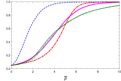
(a) $\bar{\kappa}=0$, $T=5$

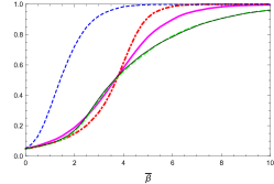
(b) $\bar{\kappa}=0$, $T=20$

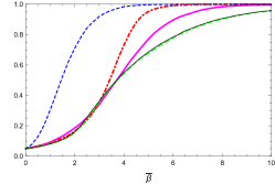
(c) $\bar{\kappa}=0$, $T=50$

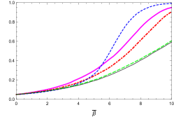
(d) $\bar{\kappa}=5$, $T=5$

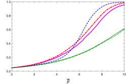
(e) $\bar{\kappa}=5$, $T=20$

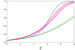
(f) $\bar{\kappa}=5$, $T=50$

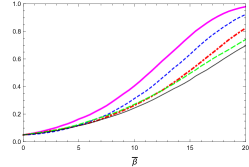
(g) $\bar{\kappa}=20$, $T=5$

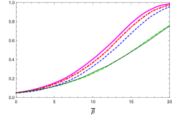
(h) $\bar{\kappa}=20$, $T=20$

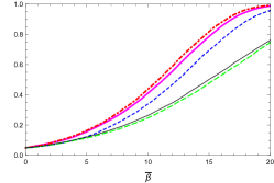
(i) $\bar{\kappa}=20$, $T=50$

Figure S.1: Power for CNST (continuous time)

OLS:   , Bonf. Q:${\color[rgb]{1,0,0}\rule[2.0pt]{4.80005pt}{1.7pt}\ \mathbf{\cdot}\ \rule[2.0pt]{4.80005pt}{1.7pt}\ }$ RLRT:      , Cauchy RT:      , NP: 

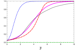
(a) $\bar{\kappa}=0$, $T=60$

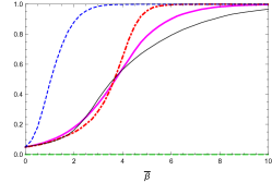
(b) $\bar{\kappa}=0$, $T=240$

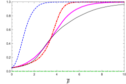
(c) $\bar{\kappa}=0$, $T=600$

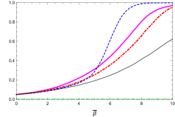
(d) $\bar{\kappa}=5$, $T=60$

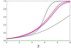
(e) $\bar{\kappa}=5$, $T=240$

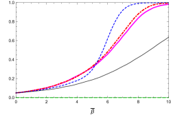
(f) $\bar{\kappa}=5$, $T=600$

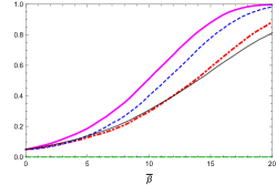
(g) $\bar{\kappa}=20$, $T=60$

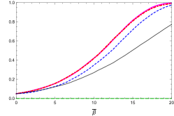
(h) $\bar{\kappa}=20$, $T=240$

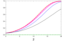
(i) $\bar{\kappa}=20$, $T=600$

Figure S.2: Power for CNST (discrete time)

OLS:   , Bonf. Q:${\color[rgb]{1,0,0}\rule[2.0pt]{4.80005pt}{1.7pt}\ \mathbf{\cdot}\ \rule[2.0pt]{4.80005pt}{1.7pt}\ }$ RLRT:      , NP: 

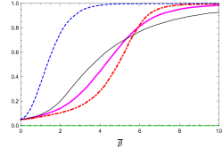
(a) $\bar{\kappa}=0$, $T=60$

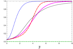
(b) $\bar{\kappa}=0$, $T=240$

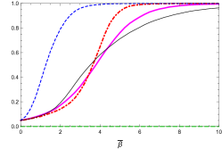
(c) $\bar{\kappa}=0$, $T=600$

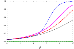
(d) $\bar{\kappa}=5$, $T=60$

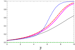
(e) $\bar{\kappa}=5$, $T=240$

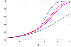
(f) $\bar{\kappa}=5$, $T=600$

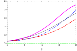
(g) $\bar{\kappa}=20$, $T=60$

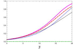
(h) $\bar{\kappa}=20$, $T=240$

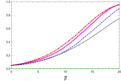
(i) $\bar{\kappa}=20$, $T=600$

Figure S.3: Power for ARCH with $\alpha=0.5773$ (discrete time)

OLS:   , Bonf. Q:${\color[rgb]{1,0,0}\rule[2.0pt]{4.80005pt}{1.7pt}\ \mathbf{\cdot}\ \rule[2.0pt]{4.80005pt}{1.7pt}\ }$ RLRT:      , NP: 

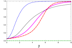
(a) $\bar{\kappa}=0$, $T=60$

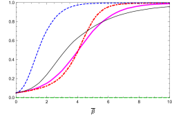
(b) $\bar{\kappa}=0$, $T=240$

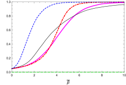
(c) $\bar{\kappa}=0$, $T=600$

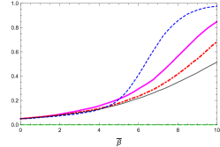
(d) $\bar{\kappa}=5$, $T=60$

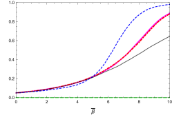
(e) $\bar{\kappa}=5$, $T=240$

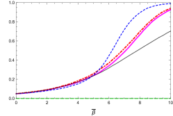
(f) $\bar{\kappa}=5$, $T=600$

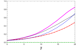
(g) $\bar{\kappa}=20$, $T=60$

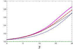
(h) $\bar{\kappa}=20$, $T=240$

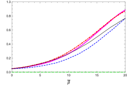
(i) $\bar{\kappa}=20$, $T=600$

Figure S.4: Power for ARCH with $\alpha=0.7325$ (discrete time)

OLS:   , Bonf. Q:${\color[rgb]{1,0,0}\rule[2.0pt]{4.80005pt}{1.7pt}\ \mathbf{\cdot}\ \rule[2.0pt]{4.80005pt}{1.7pt}\ }$ RLRT:      , NP: 

References

Applebaum, D. (2009), ‘Lévy Processes and Stochastic Calculus’. Cambridge University Press.

Bercu, B., and Touati, A. (2008), ‘Exponential inequalities for self-normalized martingales with applications’, Annals of Applied Probability 18, 1848–1869.

Kurtz, T. G. and Protter, P. (1991), ‘Weak limit theorems for stochastic integrals and stochastic differential equations’, Annals of Probability 19, 1035–1070.

Hansen, B. E. (1992), ‘Convergence to stochastic integrals for dependent heterogeneous processes’, Econometric Theory 8, 489–500.

Vogt, M. (2012), ‘Nonparametric regression for locally stationary time series’, Annals of Statistics 40, 2601–2633.

References

- (1)
- Baillie (1996) Baillie, R. T. (1996), ‘Long memory processes and fractional integration in econometrics’, Journal of Econometrics 59, 5–59.
- Bercu and Touati (2008) Bercu, B. and Touati, A. (2008), ‘Exponential inequalities for self-normalized martingales with applications’, Annals of Applied Probability 18(5), 1848–1869.
- Billingsley (1986) Billingsley, P. (1986), Convergence of Probability Measures, John Wiley & Sons.
- Brown and Ibragimov (2019) Brown, D. and Ibragimov, R. (2019), ‘Sign tests for dependent observations’, Econometrics and Statistics 10, 1–8.
- Campbell and Dufour (1995) Campbell, B. and Dufour, J.-M. (1995), ‘Exact nonparametric orthogonality and random walk tests’, Review of Economics and Statistics 77, 1–16.
- Campbell and Yogo (2006) Campbell, J. and Yogo, M. (2006), ‘Efficient tests of stock return predictability’, Journal of Financial Econometrics 81, 27–60.
- Carrasco and Chen (2002) Carrasco, M. and Chen, X. (2002), ‘Mixing and moment properties of various GARCH and stochastic volatility models’, Econometric Theory 18, 17–39.
- Cauchy (1836) Cauchy, A. (1836), ‘On a new formula for solving the problem of interpolation in a manner applicable to physical investigations’, The London, Edinburgh, and Dublin Philosophical Magazine and Journal of Science 8(49), 459–468.
- Cavaliere (2004) Cavaliere, G. (2004), ‘Testing stationarity under a permanent variance shift’, Economics Letters 82, 403–408.
- Cavaliere and Taylor (2007) Cavaliere, G. and Taylor, A. R. (2007), ‘Testing for unit roots in time series models with non-stationary volatility’, Journal of Econometrics 140, 919–947.
- Cavaliere and Taylor (2009) Cavaliere, G. and Taylor, A. R. (2009), ‘Heteroskedastic time series with a unit root’, Econometric Theory 25, 1228–1276.
- Chan and Wang (2015) Chan, N. and Wang, Q. (2015), ‘Nonlinear regressions with nonstationary time series’, Journal of Econometrics 185, 182–195.
- Chen and Deo (2009) Chen, W. and Deo, R. (2009), ‘Bias reduction and likelihood-based almost exactly sized hypothesis testing in predictive regressions using the restricted likelihood’, Econometric Theory 25, 1143–1179.
- Choi et al. (2016) Choi, Y., Jacewitz, S. and Park, J. Y. (2016), ‘A reexamination of stock return predictability’, Journal of Econometrics 192, 168–189.
- Chung and Park (2007) Chung, H. and Park, J. Y. (2007), ‘Nonstationary nonlinear heteroskedasticity in regression’, Journal of Econometrics 137, 230–259.
- Cont (2001) Cont, R. (2001), ‘Empirical properties of asset returns: Stylized facts and statistical issues’, Quantitative Finance 1, 223–236.
- Davis and Mikosch (1998) Davis, R. A. and Mikosch, T. (1998), ‘The sample autocorrelations of heavy-tailed processes with applications to ARCH’, Annals of Statistics 26, 2049–2080.
- de la Peña et al. (2003) de la Peña, V. H., Ibragimov, R. and Sharakhmetov, S. (2003), ‘On extremal distributions and sharp -bounds for sums of multilinear forms’, Annals of Probability 31, 630–675.
- de la Peña (1999) de la Peña, V. H. (1999), ‘A general class of exponential inequalities for martingales and ratios’, The Annals of Probability 27(1), 537–564.
- de la Peña and Ibragimov (2017) de la Peña, V. H. and Ibragimov, R. (2017), Sharp probability inequalities for random polynomials, generalized sample cross-moments, and Studentized processes, in I. Pinelis, ed., ‘ Inequalities and Extremal Problems in Probability and Statistics: Selected Topics’, pp. 159–187.
- Dufour and Hallin (1993) Dufour, J.-M. and Hallin, M. (1993), ‘Improved Eaton bounds for linear combinations of bounded random variables, with statistical applications’, Journal of the American Statistical Association 88, 1026–1033.
- Edelman (1990) Edelman, D. (1990), ‘An inequality of optimal order for the tail probabilities of the statistic under symmetry’, Journal of the American Statistical Association 85, 120–122.
- Efron (1969) Efron, B. (1969), ‘Student’s test under symmetry conditions’, Journal of the American Statistical Association 64, 1278–1302.
- Elliott and Stock (1994) Elliott, G. and Stock, J. H. (1994), ‘Inference in time series regression when the order of integration of a regressor is unknown’, Econometric Theory 10, 672–700.
- Embrechts et al. (1997) Embrechts, P., Klüppelberg, C. and Mikosch, T. (1997), Modelling Extremal Events for Insurance and Finance, Springer.
- Francq and Zakoïan (2006) Francq, C. and Zakoïan, J.-M. (2006), ‘Mixing properties of a general class of GARCH (1, 1) models without moment assumptions on the observed process’, Econometric Theory 22, 815–834.
- Ghysels et al. (2020) Ghysels, E., Hill, J. B. and Motegi, K. (2020), ‘Testing a large set of zero restrictions in regression models, with an application to mixed frequency Granger causality’, Journal of Econometrics 218, 633–654.
- Granger and Orr (1972) Granger, C. W. J. and Orr, D. (1972), ‘Infinite variance and research strategy in time series analysis’, Journal of the American Statistical Association 67, 275–285.
- Hansen (1992) Hansen, B. E. (1992), ‘Convergence to stochastic integrals for dependent heterogeneous processes’, Econometric Theory 8, 489–500.
- Hansen (1995) Hansen, B. E. (1995), ‘Regression with nonstationary volatility’, Econometrica 63, 1113–1132.
- Hansen and Lunde (2014) Hansen, P. R. and Lunde, A. (2014), ‘Estimating the persistence and the autocorrelation function of a time series that is measured with error’, Econometric Theory 30, 60–93.
- Harvey et al. (2019) Harvey, D. I., Leybourne, S. J. and Zu, Y. (2019), ‘Testing explosive bubbles with time-varying volatility’, Econometric Reviews 38, 1131–1151.
- Ibragimov et al. (2015) Ibragimov, M., Ibragimov, R. and Walden, J. (2015), Heavy-tailed Distributions and Robustness in Economics and Finance, Vol. 214 of Lecture Notes in Statistics, Springer.
- Ibragimov and Müller (2010) Ibragimov, R. and Müller, U. (2010), ‘-statistic Based Correlation and Heterogeneity Robust Inference’, Journal of Business & Economic Statistics 28, 453–468.
-
Ibragimov et al. (2021)
Ibragimov, R., Pedersen, R. S. and Skrobotov, A. (2021), ‘New approaches to robust inference on market
(non-)efficiency, volatility clustering and nonlinear dependence’.
Working paper, Imperial College Business School and the
University of Copenhagen.
https://papers.ssrn.com/sol3/papers.cfm?abstract_id=3580916 - Ibragimov and Phillips (2008) Ibragimov, R. and Phillips, P. C. B. (2008), ‘Regression asymptotics using martingale convergence methods’, Econometric Theory 24, 888–947.
- Jacquier et al. (2004) Jacquier, E., Polson, N. G. and Rossi, P. E. (2004), ‘Bayesian analysis of stochastic volatility models with fat-tails and correlated errors’, Journal of Econometrics 122, 185–212.
-
Kim and Phillips (2006)
Kim, C. S. and Phillips, P. C. B. (2006), ‘Log periodogram regression: The nonstationary case’.
Cowles Foundation Discussion Paper No. 1587.
https://papers.ssrn.com/sol3/papers.cfm?abstract_id=937915 - Kim and Meddahi (2020) Kim, J. and Meddahi, N. (2020), ‘‘Volatility regressions with fat tails’’, Journal of Econometrics 218, 690–713.
- Kim and Park (2017) Kim, J. and Park, J. Y. (2017), ‘Asymptotics for recurrent diffusions with application to high frequency regression’, Journal of Econometrics 196, 37–54.
- Kristensen (2009) Kristensen, D. (2009), ‘Uniform convergence rates of kernel estimators with heterogeneous dependent data’, Econometric Theory 25, 1433–1445.
- Kurtz and Protter (1991) Kurtz, T. G. and Protter, P. (1991), ‘Weak limit theorems for stochastic integrals and stochastic differential equations’, Annals of Probability 19, 1035–1070.
- Leadbetter and Rootzén (1988) Leadbetter, M. and Rootzén, H. (1988), ‘Extremal theory for stochastic processes’, Annals of Probability 16, 431–478.
- Liebscher (1996) Liebscher, E. (1996), ‘Strong convergence of sums of -mixing random variables with applications to density estimation’, Stochastic Processes and Their Applications 65, 69–80.
- Mikosch and Stărică (2000) Mikosch, T. and Stărică, C. (2000), ‘Limit theory for the sample autocorrelations and extremes of a GARCH process’, Annals of Statistics 28, 1427–1451.
-
Park (2003)
Park, J. Y. (2003), ‘Weak unit roots’, Unpublished Manuscript .
http://www.ruf.rice.edu/~econ/papers/2003papers/17park.pdf - Park and Phillips (2001) Park, J. Y. and Phillips, P. C. B. (2001), ‘Nonlinear regressions with integrated time series’, Econometrica 69, 117–161.
- Phillips (1987a) Phillips, P. C. B. (1987a), ‘Time-series regression with a unit root’, Econometrica 55, 277–301.
- Phillips (1987b) Phillips, P. C. B. (1987b), ‘Towards a unified asymptotic theory for autoregression’, Biometrika 74, 535–547.
- Phillips (1999) Phillips, P. C. B. (1999), ‘Discrete Fourier transforms of fractional processes’. Cowles Foundation Discussion Paper No. 1243.
- Phillips (2015) Phillips, P. C. B. (2015), ‘Halbert White Jr. Memorial JFEC Lecture: Pitfalls and possibilities in predictive regression’, Journal of Financial Econometrics 13, 521–555.
- Phillips and Magdalinos (2007) Phillips, P. C. B. and Magdalinos, T. (2007), ‘Limit theory for moderate deviations from a unit root’, Journal of Econometrics 136, 115–130.
- Phillips and Magdalinos (2009) Phillips, P. C. B. and Magdalinos, T. (2009), ‘Econometric inference in the vicinity of unity’, Working paper, Yale University and University of Nottingham .
- Phillips et al. (2004) Phillips, P. C. B., Park, J. Y. and Chang, Y. (2004), ‘Nonlinear instrumental variable estimation of an autoregression’, Journal of Econometrics 118, 219–246.
- Phillips and Solo (1992) Phillips, P. C. B. and Solo, V. (1992), ‘Asymptotics for linear processes’, Annals of Statistics 20, 971–1001.
- Pinelis (1994) Pinelis, I. (1994), ‘Extremal probabilistic problems and Hotelling’s test under a symmetry condition’, Annals of Statistics 22, 357–368.
- Samorodnitsky et al. (2007) Samorodnitsky, G., Rachev, S. T., Kurz-Kim, J.-R. and Stoyanov, S. V. (2007), ‘Asymptotic Distributions of Unbiased Linear Estimators in the Presence of Heavy-Tailed Stochastic Regressors and Residuals’, Probability and Mathematical Statistics 27, 275–302.
- Shephard (2020) Shephard, N. (2020), ‘An estimator for predictive regression: reliable inference for financial economics’, Working Paper, Harvard University .
- So and Shin (1999) So, B. and Shin, D. (1999), ‘Cauchy estimators for autoregressive processes with applications to unit root tests and confidence intervals’, Econometric Theory 15, 165–176.
- So and Shin (2001) So, B. and Shin, D. (2001), ‘An invariant sign tests for random walks based on recursive median adjustment’, Journal of Econometrics 102, 197–229.
- Stambaugh (1999) Stambaugh, R. F. (1999), ‘Predictive regressions’, Journal of Financial Economics 54, 375–421.
- Vogt (2012) Vogt, M. (2012), ‘Nonparametric regression for locally stationary time series’, Annals of Statistics 40, 2601–2633.
- Wang and Chan (2014) Wang, Q. and Chan, N. (2014), ‘Uniform convergence rates for a class of martingales with application in non-linear cointegrating regression’, Bernoulli 20, 207–230.
- Wang et al. (2003) Wang, Q., Lin, Y.-X. and Gulati, C. M. (2003), ‘Asymptotics for general fractionally integrated processes with applications to unit root tests’, Econometric Theory 19, 143–164.
- Xu and Guo (2022) Xu, K.-L. and Guo, J. (2022), ‘A new test for multiple predictive regression’, Journal of Financial Econometrics .
- Xu and Phillips (2008) Xu, K.-L. and Phillips, P. C. B. (2008), ‘Adaptive estimation of autoregressive models with time-varying variances’, Journal of Econometrics 142, 265–280.