Explaining $(g-2)_{\mu,e}$, the KOTO anomaly and the MiniBooNE excess in an extended Higgs model with sterile neutrinos

Abstract

We consider a simple extension of the Standard Model (SM) by a complex scalar doublet and a singlet along with three sterile neutrinos. The sterile neutrinos mix with the SM neutrinos to produce three light neutrino states consistent with the oscillation data and three heavy sterile states. The lightest sterile neutrino has lifetime longer than the age of the Universe and can provide correct dark matter relic abundance. Utilizing tree-level flavor changing interactions of a light scalar with mass $\sim\mathcal{O}(100)$ MeV along with sterile neutrinos, we can explain the anomalous magnetic moments of both muon and electron, KOTO anomalous events and the MiniBooNE excess simultaneously.

I Introduction

The Standard Model (SM) of particle physics is a very successful, mathematically consistent theory of the known elementary particles. Most of the SM predictions are consistent with the experimental data. However, some theoretical puzzles and experimental results cannot be explained solely based on the SM. These are the hints that we need some new physics beyond the SM. The need for new physics beyond the SM is well established in the neutrino sector of the SM where the neutrino oscillation data Fukuda et al. (1998); Ahmad et al. (2002) definitely require at least two neutrinos to have non-zero masses. On the other hand, the SM does not provide any dark matter (DM) candidate which could explain the observed DM content of the Universe Aghanim et al. (2018). In addition to the neutrino and DM puzzles, a few other experimental results associated with the quarks and charged leptons also pose challenges to the SM.

The anomalous magnetic moment of the muon is one of the long-standing deviations of the experimental data from the theoretical predictions of the SM. There exists a 3.7 $\sigma$ discrepancy between the experimental results Bennett et al. (2006); Tanabashi et al. (2018) and theoretical predictions Davier et al. (2017); Blum et al. (2018); Keshavarzi et al. (2018); Davier et al. (2020). This was recently accompanied by a 2.4 $\sigma$ discrepancy between the experimental Hanneke et al. (2011, 2008) and theoretical Aoyama et al. (2018) values of the anomalous magnetic moment of the electron due to a recent precise measurement of the fine structure constant Parker et al. (2018). It is interesting to note that the deviations are in opposite directions, and $\Delta a_{e}/\Delta a_{\mu}$ does not follow the lepton mass scaling $m_{e}^{2}/m_{\mu}^{2}\sim 2.25\times 10^{-5}$. It would require a model with new flavor structure in the leptonic sector to explain these discrepancies. Universal flavor structure requires very large Yukawa coupling to explain the anomalies Hiller et al. (2019). More data is needed to confirm the $\Delta a_{e}$ discrepancy. There will be new results for the $a_{\mu}$ measurement from the Fermilab soon. Very recently, the lattice calculation for the hadronic light-by-light scattering contribution confirms the $\Delta a_{\mu}$ discrepancy Blum et al. (2020). Recently, the measurement of the radiative corrections to the pion form factor also confirm the need of a beyond SM explanation of $a_{\mu}$ Campanario et al. (2019).

Any observations of the flavor changing rare decays of kaons also indicate new physics beyond the SM. One very interesting development in this topic is the recent results from the KOTO experiment which is indicating that $K_{L}\rightarrow\pi^{0}\bar{\nu}\nu$ decay takes place at a higher rate compared to the SM prediction Shinohara (2019); Lin (2019). The branching ratio is estimated to be at least two orders of magnitude larger than the SM prediction Buras et al. (2015). Any new physics explanation of this excess is, however, constrained by the charged kaon decay mode $K^{+}\rightarrow\pi^{+}\nu\bar{\nu}$ and $K^{+}\rightarrow\pi^{+}X$ which are being investigated at NA62 Ruggiero (2019) and E949 Artamonov et al. (2009) experiments, respectively. The new physics to explain the anomaly also requires flavor violating interactions in the quark sector.

The interesting question is can any simple extension of the SM explain all these observations? In an attempt to find the answer to this question, we propose a simple extension of the SM which contains an additional scalar doublet, a singlet, and three sterile neutrinos. This Higgs sector extension is simple, well-motivated, and is associated with the electroweak sector of the SM Branco et al. (2012). We investigate the most general renormalized scalar potential utilizing the electroweak symmetry breaking and explore the parameter space associated with the masses and mixings of the Higgs bosons. The interesting feature of this parameter space is the emergence of a light scalar that has tree-level flavor violating couplings to the SM fermions. Further, the sterile neutrinos would help us to realize tiny neutrino masses utilizing type I seesaw in this model. The lightest sterile neutrino can be a viable DM candidate. Utilizing the flavor violation in the lepton sector, we explain the $g-2$ of both muon and electron. The quark sector flavor violation leads to tree level decays of kaon into pion and dark matter pair which will mimic the $K_{L}\rightarrow\pi^{0}\bar{\nu}\nu$ decay channel inside the KOTO detector and help to explain the KOTO anomaly.

In addition to the light neutrino masses and KOTO anomaly, the existence of the sterile neutrinos would help us to explain two other puzzles. One of them is the DM content of the Universe which can be explained by the DM candidate in this model, i.e., the lightest sterile neutrino. The other one is the recent MiniBooNE observation where the data exhibits a 4.8 $\sigma$ excess Aguilar-Arevalo et al. (2018, 2020) of events over the known background. This excess can be explained with the muon neutrino getting upscattered to a heavy sterile neutrino due to the light scalar.

Finally, the parameter space of this light scalar with couplings to leptons and quarks is constrained by various proton, electron beam dump, and collider experiments, lepton flavor violating decays, kaon mixing, and astrophysical data. We explore various constraints and determine the allowed parameter space where all the anomalies can be explained simultaneously. We also make predictions of this allowed parameter space for various ongoing and upcoming experiments.

The rest of the paper is organized as follows: In Sec. II we discuss the model by defining necessary parameters and interaction terms. The origin of neutrino mass is presented in Sec. III. In Sec. IV, we discuss the possibility of the lightest sterile neutrino as a DM candidate. We generate a viable physical scalar spectrum in Sec. V. In Sec. VI, we study the anomalous magnetic moments of the electron and muon and allowed parameter space. In Sec. VII, we discuss the allowed parameter space associated with the KOTO anomaly. In Sec. VIII V, we discuss the recent MiniBooNE observation. We summarize our analysis in Sec. IX by showing a few benchmark points (BP) which explain all the anomalies after satisfying all other experimental data. We provide additional pieces of information in the Appendices.

II model

The scalar sector of the SM has the simplest possible structure with one scalar doublet Higgs (1964, 1966); Englert and Brout (1964); Guralnik et al. (1964); Kibble (1967). Two-Higgs-doublet model (2HDM) Lee (1973); Branco et al. (2012) and its singlet/triplet extensions are well motivated extension of the SM scalar sector He et al. (2009); Grzadkowski and Osland (2010); Logan (2011); Boucenna and Profumo (2011); He et al. (2012); Bai et al. (2013); He and Tandean (2013); Cai and Li (2013); Guo and Kang (2015); Wang and Han (2014); Drozd et al. (2014); Campbell et al. (2015); Drozd et al. (2016); von Buddenbrock et al. (2016); Muhlleitner et al. (2017); Liu et al. (2016). In this work, we consider a simple extension of the CP-conserving 2HDM by adding one complex scalar singlet. In addition to this, we extend the SM fermion sector by adding three right-handed sterile neutrinos $n^{\prime}_{R_{i}}$ with $i=1,2,3$ to explain the observed neutrino masses and mixings. The quantum numbers of the scalars under the SM gauge group $SU(2)_{L}\times U(1)_{Y}$ are

$$\phi_{1}\sim(2,1/2),~{}~{}~{}~{}~{}\phi_{2}\sim(2,1/2),~{}~{}~{}~{}~{}\phi_{S}\sim(1,0)~{},~{}\,$$ (1)

and the definition of the electric charge is $Q\equiv T_{3}+Y$.

In general, the scalar sector can be CP-violating. For simplicity, we assume that the scalar sector respects the CP symmetry. Also, we do not impose any discrete symmetry. The most general renormalizable and CP-conserving scalar potential can be written as follows

$$V=m_{1}^{2}\phi_{1}^{\dagger}\phi_{1}+m_{2}^{2}\phi_{2}^{\dagger}\phi_{2}+m_{12}^{2}(\phi_{1}^{\dagger}\phi_{2}+\phi_{2}^{\dagger}\phi_{1})+m_{S}^{2}\phi_{S}^{\dagger}\phi_{S}-m_{S^{\prime}}^{2}(\phi_{S}^{2}+{\phi^{\dagger 2}_{S}})+m_{1S}(\phi_{1}^{\dagger}\phi_{1}\phi_{S}+\phi_{1}^{\dagger}\phi_{1}\phi_{S}^{\dagger})+m_{2S}(\phi_{2}^{\dagger}\phi_{2}\phi_{S}+\phi_{2}^{\dagger}\phi_{2}\phi_{S}^{\dagger})+\frac{\lambda_{1}}{2}(\phi_{1}^{\dagger}\phi_{1})^{2}+\frac{\lambda_{2}}{2}(\phi_{2}^{\dagger}\phi_{2})^{2}+\frac{\lambda_{S}}{2}(\phi_{S}^{\dagger}\phi_{S})^{2}+\lambda_{3}(\phi_{1}^{\dagger}\phi_{1})(\phi_{2}^{\dagger}\phi_{2})+\lambda_{4}(\phi_{1}^{\dagger}\phi_{2})(\phi_{2}^{\dagger}\phi_{1})+\lambda_{5}\left[(\phi_{1}^{\dagger}\phi_{2})^{2}+(\phi_{2}^{\dagger}\phi_{1})^{2}\right]+\lambda_{6}\left[(\phi_{1}^{\dagger}\phi_{1})(\phi_{1}^{\dagger}\phi_{2})+(\phi_{1}^{\dagger}\phi_{1})(\phi_{2}^{\dagger}\phi_{1})\right]+\lambda_{7}\left[(\phi_{2}^{\dagger}\phi_{2})(\phi_{1}^{\dagger}\phi_{2})+(\phi_{2}^{\dagger}\phi_{2})(\phi_{2}^{\dagger}\phi_{1})\right]+\lambda_{1S}(\phi_{1}^{\dagger}\phi_{1})(\phi_{S}^{\dagger}\phi_{S})+\lambda_{2S}(\phi_{2}^{\dagger}\phi_{2})(\phi_{S}^{\dagger}\phi_{S})+\lambda_{12S}\left[(\phi_{1}^{\dagger}\phi_{2})(\phi_{S}^{\dagger}\phi_{S})+(\phi_{2}^{\dagger}\phi_{1})(\phi_{S}^{\dagger}\phi_{S})\right]+m_{12S}(\phi_{1}^{\dagger}\phi_{2}\phi_{S}+\phi_{S}^{\dagger}\phi_{2}^{\dagger}\phi_{1})~{}.~{}\,$$ (2)

We choose to work in the Higgs basis Georgi and Nanopoulos (1979); Botella and Silva (1995); Lavoura and Silva (1994); Donoghue and Li (1979); Lavoura (1994), where only one of the doublet $\phi_{1}$ gets a vacuum expectation value (vev), $\braket{\phi_{1}}=v/\sqrt{2}$. The details about the Higgs basis for the scalar structure of our model is given in Appendix A. The doublet $\phi_{1}$ completely controls the spontaneous electroweak gauge symmetry breaking and the mass generations of the fermions and gauge bosons. While the other doublet and the singlet are ordinary scalars. In the following, we analyze the scalar sector in the Higgs basis. After the spontaneous symmetry breaking, we can write the scalars as

$$\phi_{1} \sim\left(\begin{array}[]{c}{G}^{+}\\ \frac{1}{\sqrt{2}}(v+\rho_{1}+iG_{0})\end{array}\right),\phi_{2}\sim\left(\begin{array}[]{c}{\phi_{2}}^{+}\\ \frac{1}{\sqrt{2}}(\rho_{2}+i\eta_{2})\end{array}\right),~{}~{}~{}~{}$$ (6)

$$\phi_{S} \sim\frac{1}{\sqrt{2}}(\rho_{S}+i\eta_{S})~{}.~{}\,$$ (7)

The extremization of the potential in Eq. 2 gives the following conditions

$$m_{1}^{2}+\frac{\lambda_{1}v^{2}}{2} = 0~{},~{}\,$$ (8)

$$m_{12}^{2}+\frac{\lambda_{6}v^{2}}{2} = 0~{}.~{}\,$$ (9)

Eq. 9 makes sure that the $\phi_{2}$ does not get a vev. From the minimizing conditions, we further get

$$\lambda_{1} >0,~{}~{}~{}~{}m_{1}^{2}<0,~{}~{}~{}\lambda_{5}>0,~{}~{}~{}\lambda_{6}>0,~{}~{}~{}m_{12}^{2}<0,$$ (10)

$$m_{12S} >0,~{}~{}~{}m_{1S}=0~{}.~{}\,$$

The vev of $\phi_{S}$ is zero due to $m_{1S}=0$. Therefore, the total number of free parameters in the scalar sectors is 17 including the vev $v$. The total number of scalar degrees of freedom (dof) is 10. Three dof get eaten to give mass to $W^{\pm}~{}\mbox{and}~{}Z$ gauge bosons. The remaining 7 are physical Higgs. In the Higgs basis, $G^{\pm}$ and $G_{0}$ become the Goldstone bosons. $\phi_{2}^{\pm}$ gives two charged physical Higgs $h^{\pm}$. CP-even states $\rho_{1}$, $\rho_{2}$ and $\rho_{S}$ mix to give three neutral physical scalars $h$, $h_{1}$ and $h_{2}$. We identify the $h$ as the SM Higgs boson. The CP-odd states $\eta_{2}$ and $\eta_{S}$ mix and gives two neutral physical pseudoscalar $s_{1}$ and $s_{2}$.

The physical charged scalar mass is given by

$$m_{h^{\pm}}^{2}=m_{2}^{2}+\frac{\lambda_{3}v^{2}}{2}~{}.~{}\,$$ (11)

The mixing of the three CP-even neutral scalars $\rho_{1}$, $\rho_{2}$ and $\rho_{S}$ is

$$V^{\rho}_{mass}=\frac{1}{2}\left(\rho_{1}~{}~{}~{}\rho_{2}~{}~{}~{}\rho_{S}\right)~{}\left(M^{2}_{\rho}\right)_{3\times 3}~{}\left(\begin{array}[]{c}\rho_{1}\\ \rho_{2}\\ \rho_{S}\end{array}\right)~{},~{}\,$$ (12)

where the $3\times 3$ mass square matrix $M^{2}_{\rho}$ is

$$M^{2}_{\rho}=\left(\begin{array}[]{ccc}\lambda_{1}v^{2}&\lambda_{6}v^{2}&0\\ \lambda_{6}v^{2}&m_{2}^{2}+\frac{\lambda^{+}_{345}v^{2}}{2}&\frac{m_{12S}v}{\sqrt{2}}\\ 0&\frac{m_{12S}v}{\sqrt{2}}&m_{S}^{2}-2m_{S^{\prime}}^{2}+\frac{\lambda_{8}v^{2}}{2}\end{array}\right)~{}.~{}\,$$ (13)

Here, we have used Eq. 9 to simplify terms in the mass squared matrix and defined $\lambda^{+}_{345}\equiv\lambda_{3}+\lambda_{4}+\lambda_{5}$. We get three physical scalars from this mixing, $h$, $h_{1}$ and $h_{2}$ with mass squared $m_{h}^{2},m_{h_{1}}^{2}$ and $m_{h_{2}}^{2}$, respectively. The fields in the mass basis, $h,h_{1}$ and $h_{2}$ are related to those in the interaction basis, $\rho_{1},\rho_{2}$ and $\rho_{S}$ by a $3\times 3$ rotation matrix ${U_{R}}_{3\times 3}(\theta_{i})$ which can be parametrized with three Euler angles $\theta_{1},\theta_{2}~{}\mbox{and}~{}\theta_{3}$. We write $U_{R}$ as follows

$$U_{R} = \left(\begin{array}[]{ccc}c_{11}&c_{12}&c_{13}\\ c_{21}&c_{22}&c_{23}\\ c_{31}&c_{32}&c_{33}\end{array}\right)~{},~{}\,$$ (17)

where $\rho_{i}={U_{R}}_{ij}h_{j}$. The quantities $c_{ij}$ are functions of $\cos\theta_{k}$ and $\sin\theta_{k}$ ($k=1,2,3$). The interaction states can be written in terms of the physical states as

$$\rho_{1} = c_{11}h_{2}+c_{12}h+c_{13}h_{1}~{},~{}\,$$

$$\rho_{2} = c_{21}h_{2}+c_{22}h+c_{23}h_{1}~{},~{}\,$$

$$\rho_{S} = c_{31}h_{2}+c_{32}h+c_{33}h_{1}~{}.~{}\,$$ (18)

The mixing of the two CP-odd neutral scalars $\eta_{2}$-$\eta_{S}$ can be written as

$$V^{\eta}_{mass}=\frac{1}{2}\left(\eta_{2}~{}~{}~{}\eta_{S}\right)\left(M^{2}_{\eta}\right)_{2\times 2}\left(\begin{array}[]{c}\eta_{2}\\ \eta_{S}\end{array}\right)~{},~{}\,$$ (21)

where the $2\times 2$ mass square matrix $M^{2}_{\eta}$ is given by

$$M^{2}_{\eta}=\left(\begin{array}[]{cc}m_{2}^{2}+\frac{\lambda^{-}_{345}v^{2}}{2}&-\frac{m_{12S}v}{\sqrt{2}}\\ -\frac{m_{12S}v}{\sqrt{2}}&m_{S}^{2}+2m_{S^{\prime}}^{2}+\frac{\lambda_{8}v^{2}}{2}\end{array}\right)~{},~{}\,$$ (22)

where we define $\lambda^{-}_{345}\equiv\lambda_{3}+\lambda_{4}-\lambda_{5}$. From the above mixing, we get two physical neutral pseudoscalar

$$\left(\begin{array}[]{c}s_{1}\\ s_{2}\end{array}\right)=\left(\begin{array}[]{cc}\cos\alpha&-\sin\alpha\\ \sin\alpha&\cos\alpha\end{array}\right)\left(\begin{array}[]{c}\eta_{2}\\ \eta_{S}\end{array}\right)~{},~{}\,$$ (23)

where the mixing angle is given by

$$\tan 2\alpha=\frac{m_{12S}v/\sqrt{2}}{m_{11}^{2}-m_{22}^{2}}$$ (24)

with the corresponding mass squared

$$m_{s_{1}}^{2}=\frac{1}{2}(m^{2}_{11}+m^{2}_{22})-\frac{1}{2}\sqrt{(m^{2}_{11}-m^{2}_{22})^{2}+\frac{m_{12S}^{2}v^{2}}{2}}$$ (25)

and

$$m_{s_{2}}^{2}=\frac{1}{2}(m^{2}_{11}+m^{2}_{22})+\frac{1}{2}\sqrt{(m^{2}_{11}-m^{2}_{22})^{2}+\frac{m_{12S}^{2}v^{2}}{2}}~{},~{}\,$$ (26)

respectively, where

$$m^{2}_{11}=\frac{1}{2}\left(m_{2}^{2}+\frac{\lambda_{3}v^{2}}{2}+\frac{\lambda_{4}v^{2}}{2}-\frac{\lambda_{5}v^{2}}{2}\right)$$ (27)

and

$$m^{2}_{22}=\frac{1}{2}\left(m_{S}^{2}+2m_{S^{\prime}}^{2}+\frac{\lambda_{8}v^{2}}{2}\right)~{}.~{}\,$$ (28)

The interaction states can be written in terms of the mass eigenstates as

$$\eta_{2} = \cos\alpha~{}s_{1}+\sin\alpha~{}s_{2}~{},~{}\,$$

$$\eta_{S} = -\sin\alpha~{}s_{1}+\cos\alpha~{}s_{2}~{}.~{}\,$$ (29)

Both scalar doublets interact with all the fermions in the interaction basis, while the singlet scalar only interacts with the sterile neutrinos. The masses of the fermions come from the interactions with $\phi_{1}$. The couplings of $\phi_{2}$ to the fermions are unconstrained and do not need to respect the SM fermion flavor symmetry. Therefore, the interactions of the fermions with the neutral components of $\phi_{2}$ can generate the tree-level flavor-changing neutral current (FCNC), which would be useful to explain the KOTO anomaly and g-2 of the electron. The fermions can interact with the singlet scalar through the scalar mixings discussed above. The complete Yukawa sector Lagrangian in the interaction basis is

$$-\mathcal{L} = \bar{q}^{\prime}_{L_{i}}(y^{\prime}_{1d})_{ij}d^{\prime}_{R_{j}}\phi_{1}+\bar{q}^{\prime}_{L_{i}}(y^{\prime}_{1u})_{ij}u^{\prime}_{R_{j}}\tilde{\phi_{1}}$$ (30)

$$+ \bar{l}^{\prime}_{L_{i}}(y^{\prime}_{1e})_{ij}e^{\prime}_{R_{j}}\phi_{1}+\bar{l}^{\prime}_{L_{i}}(y^{\prime}_{1n})_{ij}n^{\prime}_{R_{j}}\tilde{\phi_{1}}$$

$$+ \bar{q}^{\prime}_{L_{i}}(y^{\prime}_{2d})_{ij}d^{\prime}_{R_{j}}\phi_{2}+\bar{q}^{\prime}_{L_{i}}(y^{\prime}_{2u})_{ij}u^{\prime}_{R_{j}}\tilde{\phi_{2}}$$

$$+ \bar{l}^{\prime}_{L_{i}}(y^{\prime}_{2e})_{ij}e^{\prime}_{R_{j}}\phi_{2}+\bar{l}^{\prime}_{L_{i}}(y^{\prime}_{2n})_{ij}n^{\prime}_{R_{j}}\tilde{\phi_{2}}$$

$$+ \bar{n}^{\prime c}_{R_{i}}(y^{\prime}_{sn})_{ij}n^{\prime}_{R_{j}}\phi_{S}+\frac{1}{2}\bar{n}^{\prime c}_{R_{i}}M^{\prime}_{ij}n^{\prime}_{R_{j}}+H.c.~{},~{}\,$$

where $i,j$ are the family indices, $i,j=1,2,3$, and $a,b=1,2$. The primed fermions are the fermions in the interaction basis. The first four terms give the down-type quark masses, up-type quark masses, charged lepton masses, and Dirac mass terms of neutrino, respectively. The last term gives the Majorana mass terms for the right-handed neutrinos. In general, all the Yukawa couplings are $3\times 3$ complex matrices.

In general, the $3\times 3$ Yukawa matrices $y^{\prime}_{1d}$, $y^{\prime}_{1u}$, $y^{\prime}_{1e}$ and $y^{\prime}_{1n}$, and the mass matrix $M^{\prime}_{ij}$ can be diagonalized through biunitary transformations as follows

$$U^{\dagger}_{d_{L}}y^{\prime}_{1d}U_{d_{R}}=y_{1d},~{}~{}~{}~{}~{}\mbox{with}~{}~{}~{}(y_{1d})_{ij}=(y_{1d})_{ii}\delta_{ij}~{},~{}\,$$ (31)

$$U^{\dagger}_{u_{L}}y^{\prime}_{1u}U_{u_{R}}=y_{1u},~{}~{}~{}~{}~{}\mbox{with}~{}~{}~{}(y_{1u})_{ij}=(y_{1u})_{ii}\delta_{ij}~{},~{}\,$$ (32)

$$U^{\dagger}_{e_{L}}y^{\prime}_{1e}U_{e_{R}}=y_{1e},~{}~{}~{}~{}~{}\mbox{with}~{}~{}~{}(y_{1e})_{ij}=(y_{1e})_{ii}\delta_{ij}~{},~{}\,$$ (33)

$$U^{\dagger}_{\nu_{L}}y^{\prime}_{1n}U_{n_{R}}=y_{1n},~{}~{}~{}~{}~{}\mbox{with}~{}~{}~{}(y_{1n})_{ij}=(y_{1n})_{ii}\delta_{ij}~{},~{}\,$$ (34)

$$U^{\dagger}_{n_{R}}M^{\prime}U_{n_{R}}=M,~{}~{}~{}~{}~{}\mbox{with}~{}~{}~{}M_{ij}=M_{ii}\delta_{ij}~{},~{}\,$$ (35)

where $U_{d_{L}}$, $U_{d_{R}}$, $U_{u_{L}}$, $U_{u_{R}}$, $U_{e_{L}}$, $U_{e_{R}}$, $U_{\nu_{L}}$ and $U_{n_{R}}$ are eight appropriate $3\times 3$ unitary matrices. These matrices can be used to define the physical states of the fermions,

$$d_{L_{i}}=(U^{\dagger}_{d_{L}})_{ij}{d}^{\prime}_{L_{j}},~{}~{}~{}~{}~{}~{}~{}~{}~{}~{}~{}~{}~{}d_{R_{i}}=(U^{\dagger}_{d_{R}})_{ij}{d}^{\prime}_{R_{j}}~{},~{}\,$$ (36)

$$u_{L_{i}}=(U^{\dagger}_{u_{L}})_{ij}{u}^{\prime}_{L_{j}},~{}~{}~{}~{}~{}~{}~{}~{}~{}~{}~{}~{}~{}u_{R_{i}}=(U^{\dagger}_{u_{R}})_{ij}{u}^{\prime}_{R_{j}}~{},~{}\,$$ (37)

$$e_{L_{i}}=(U^{\dagger}_{e_{L}})_{ij}{e}^{\prime}_{L_{j}},~{}~{}~{}~{}~{}~{}~{}~{}~{}~{}~{}~{}~{}e_{R_{i}}=(U^{\dagger}_{e_{R}})_{ij}{e}^{\prime}_{R_{j}}~{},~{}\,$$ (38)

$$\nu_{L_{i}}=(U^{\dagger}_{\nu_{L}})_{ij}{\nu}^{\prime}_{L_{j}},~{}~{}~{}~{}~{}~{}~{}~{}~{}~{}~{}~{}~{}n_{R_{i}}=(U^{\dagger}_{n_{R}})_{ij}{n}^{\prime}_{R_{j}}~{}.~{}\,$$ (39)

We also define the following matrices,

$$(y_{2d})_{ij} = (U^{\dagger}_{d_{L}})_{ik}(y^{\prime}_{2d})_{kl}(U_{d_{R}})_{lj}~{},~{}\,$$ (40)

$$(y_{2u})_{ij} = (U^{\dagger}_{u_{L}})_{ik}(y^{\prime}_{2u})_{kl}(U_{u_{R}})_{lj}~{},~{}\,$$ (41)

$$(y_{2e})_{ij} = (U^{\dagger}_{e_{L}})_{ik}(y^{\prime}_{2e})_{kl}(U_{e_{R}})_{lj}~{},~{}\,$$ (42)

$$(y_{2n})_{ij} = (U^{\dagger}_{\nu_{L}})_{ik}(y^{\prime}_{2n})_{kl}(U_{n_{R}})_{lj}~{},~{}\,$$ (43)

$$(y_{sn})_{ij} = (U^{\dagger}_{n_{R}})_{ik}(y^{\prime}_{sn})_{kl}(U_{n_{R}})_{lj}~{}.~{}\,$$ (44)

Using the definitions Eq. 31-44 and the physical scalar states, the Eq. 30 can be written compactly as follows

$$-\mathcal{L} = (m_{f})_{i}\bar{f}_{i}f_{i}+(m_{\nu_{d}})_{i}(\bar{\nu}_{L_{i}}n_{R_{i}}+\bar{n}_{R_{i}}\nu_{L_{i}})$$ (45)

$$+ \frac{1}{2}M_{i}(\bar{n}^{c}_{R_{i}}n_{R_{i}}+\bar{n}_{R_{i}}n^{c}_{R_{i}})$$

$$+ \bar{\nu}_{L_{i}}(U^{\dagger}_{PMNS})_{ik}(y_{2e})_{kj}e_{R_{j}}h^{+}$$

$$+ \bar{e}_{R_{i}}(y_{2e})_{ik}(U_{PMNS})_{kj}\nu_{L_{j}}h^{-}$$

$$- \bar{e}_{L_{i}}(U_{PMNS})_{ik}(y_{2n})_{kj}n_{R_{j}}h^{-}$$

$$- \bar{n}_{R_{i}}(y_{2n})_{ik}(U^{\dagger}_{PMNS})_{kj}e_{L_{j}}h^{+}$$

$$+ \bar{u}_{i}[(U_{CKM})_{ik}(y_{2d})_{kj}P_{R}-(y_{2u})_{ik}(U_{CKM})_{kj}P_{L}]d_{j}h^{+}$$

$$+ \bar{d}_{i}[(y_{2d})_{ik}(U^{\dagger}_{CKM})_{kj}P_{L}-(U^{\dagger}_{CKM})_{ik}(y_{2u})_{kj}P_{R}]u_{j}h^{-}$$

$$+ \bar{f}_{i}(y_{f\phi})_{ij}f_{j}\phi+(y_{n\phi})_{ij}(\bar{\nu}_{L_{i}}n_{R_{j}}+\bar{n}_{R_{i}}\nu_{L_{j}})\phi$$

$$+ (y_{nn\phi})_{ij}(\bar{n}^{c}_{R_{i}}n_{R_{j}}+\bar{n}_{R_{i}}n^{c}_{R_{j}})\phi~{},~{}\,$$

where $f=d,u,e$; $\phi=h,h_{1},h_{2},s_{1},s_{2}$ and $(m_{f})_{i}=(y_{1f})_{i}v/\sqrt{2}$. The Dirac mass matrix of neutrinos is defined as $(m_{\nu_{d}})_{i}=(y_{1n})_{ii}v/\sqrt{2}$ while $M_{i}=M_{ii}\delta_{ij}$ is the Majorana mass matrix. The definitions of the Cabibbo-Kobayashi-Maskawa (CKM) and Pontecorvo-Maki-Nakagawa-Sakata (PMNS) matrices are

$$U_{CKM} = U^{\dagger}_{u_{L}}U_{d_{L}}~{},~{}\,$$ (46)

$$U_{PMNS} = U^{\dagger}_{e_{L}}U_{\nu_{L}}~{}.~{}\,$$ (47)

The couplings $y_{f\phi}$ are defined as

$$(y_{fh_{2}})_{ij} = \frac{(m_{f})_{i}}{v}c_{11}\delta_{ij}+\frac{(y_{2f})_{ij}}{\sqrt{2}}c_{21}~{},~{}\,$$

$$(y_{fh})_{ij} = \frac{(m_{f})_{i}}{v}c_{12}\delta_{ij}+\frac{(y_{2f})_{ij}}{\sqrt{2}}c_{22}~{},~{}\,$$

$$(y_{fh_{1}})_{ij} = \frac{(m_{f})_{i}}{v}c_{13}\delta_{ij}+\frac{(y_{2f})_{ij}}{\sqrt{2}}c_{23}~{},~{}\,$$

$$(y_{fs_{1}})_{ij} = i\frac{(y_{2f})_{ij}}{\sqrt{2}}\cos{\alpha}~{},~{}\,$$

$$(y_{fs_{2}})_{ij} = i\frac{(y_{2f})_{ij}}{\sqrt{2}}\sin{\alpha}~{}.~{}\,$$ (48)

The couplings $y_{n\phi}$ of active-sterile neutrino states with the scalars are defined as

$$(y_{nh_{2}})_{ij} = \frac{(m_{\nu_{D}})_{i}}{v}c_{11}\delta_{ij}+\frac{(y_{2n})_{ij}}{\sqrt{2}}c_{21}~{},~{}\,$$

$$(y_{nh})_{ij} = \frac{(m_{\nu_{D}})_{i}}{v}c_{12}\delta_{ij}+\frac{(y_{2n})_{ij}}{\sqrt{2}}c_{22}~{},~{}\,$$

$$(y_{nh_{1}})_{ij} = \frac{(m_{\nu_{D}})_{i}}{v}c_{13}\delta_{ij}+\frac{(y_{2n})_{ij}}{\sqrt{2}}c_{23}~{},~{}\,$$

$$(y_{ns_{1}})_{ij} = i\frac{(y_{2n})_{ij}}{\sqrt{2}}\cos{\alpha}~{},~{}\,$$

$$(y_{ns_{2}})_{ij} = i\frac{(y_{2n})_{ij}}{\sqrt{2}}\sin{\alpha}~{}.~{}\,$$ (49)

And the couplings between two sterile neutrinos and the scalars, $y_{nn\phi}$ are defined as

$$(y_{nnh_{2}})_{ij} = \frac{(y_{sn})_{ij}}{\sqrt{2}}c_{31}~{},~{}\,$$

$$(y_{nnh})_{ij} = \frac{(y_{sn})_{ij}}{\sqrt{2}}c_{32}~{},~{}\,$$

$$(y_{nnh_{1}})_{ij} = \frac{(y_{sn})_{ij}}{\sqrt{2}}c_{33}~{},~{}\,$$

$$(y_{nns_{1}})_{ij} = -i\frac{(y_{sn})_{ij}}{\sqrt{2}}\sin{\alpha}~{},~{}\,$$

$$(y_{nns_{2}})_{ij} = i\frac{(y_{sn})_{ij}}{\sqrt{2}}\cos{\alpha}~{}.~{}\,$$ (50)

So far, we have presented the general framework of the model without assuming any particular parameter space in mind. In the next three sections, Secs. III-V, we want to generate a particular parameter space relevant for the rest of the paper.

III neutrino masses and mixings

We study the mixings between the active and sterile neutrino states and the generation of neutrino masses in this section. The sterile neutrinos will generically mix with the active states and produce six neutrino eigenstates. The masses of the three lightest eigenstates can be determined by the type-I seesaw mechanism Minkowski (1977); Yanagida (1979); Gell-Mann et al. (1979); Mohapatra and Senjanovic (1980). The part of the Lagrangian from the Eq. 45, which is responsible for the masses of the neutrinos, is given by

$$-\mathcal{L}_{\text{neutrino}} = (m_{\nu_{d}})_{i}(\bar{\nu}_{L_{i}}n_{R_{i}}+\bar{n}_{R_{i}}\nu_{L_{i}})$$ (55)

$$+\frac{1}{2}M_{i}(\bar{n}^{c}_{R_{i}}n_{R_{i}}+\bar{n}_{R_{i}}n^{c}_{R_{i}})$$

$$= \frac{1}{2}\left(\bar{\nu}^{C}_{L_{i}}~{}\bar{\eta}_{R_{i}}\right)\left(\begin{array}[]{cc}0&(m^{T}_{\nu_{d}})_{i}\\ (m_{\nu_{d}})_{i}&M_{i}\end{array}\right)\left(\begin{array}[]{c}\nu_{L_{i}}\\ n^{C}_{R_{i}}\end{array}\right)$$

$$+\text{H.c.}~{}.~{}\,$$ (56)

The Dirac-Majorana mass matrix of neutrinos is given the $6\times 6$ matrix

$$M^{D+M}_{i}=\left(\begin{array}[]{cc}0&(m^{T}_{\nu_{d}})_{i}\\ \\ (m_{\nu_{d}})_{i}&M_{i}\end{array}\right)~{}.~{}\,$$ (57)

The mass matrix $M^{D+M}_{i}$ can be diagonalized by blocks Kanaya (1980); Schechter and Valle (1982), up to corrections at the order of $M_{i}^{-1}(m_{\nu_{d}})_{i}$, under the assumption that all the eigenvalues of $M_{i}$ are much larger than the eigenvalues of $(m_{\nu_{d}})_{i}$

$$\mathcal{W}^{T}M^{D+M}_{i}\mathcal{W}\simeq\left(\begin{array}[]{cc}(M_{\text{light}})_{i}&0\\ \\ 0&(M_{\text{heavy}})_{i}\end{array}\right)~{},~{}\,$$ (58)

where the $6\times 6$ diagonalizing matrix $\mathcal{W}$ is given by

$$\mathcal{W}\simeq\left(\begin{array}[]{cc}1-\frac{1}{2}RR^{\dagger}&R^{\dagger}\\ \\ -R&1-\frac{1}{2}R^{\dagger}R\end{array}\right)$$ (59)

with $R=M_{i}^{-1}(m_{\nu_{d}})_{i}$. The $3\times 3$ light and heavy neutrino mass matrices are given by

$$m_{\nu_{i}} = (M_{\text{light}})_{i}=-(m^{T}_{\nu_{d}})_{i}M_{i}^{-1}(m_{\nu_{d}})_{i}~{},~{}\,$$

$$m_{n_{i}} = (M_{\text{heavy}})_{i}=M_{i}~{}.~{}\,$$ (60)

We redefine $\nu_{i}$ and $n_{i}$ as the physical light active neutrinos and heavy sterile neutrinos, respectively. The masses $m_{\nu_{i}}$ are not known experimentally because the neutrino oscillations are only sensitive to the differences, $m_{\nu_{i}}^{2}-m_{\nu_{j}}^{2}$. In normal hierarchy scenario, $i.e.$, assuming $m_{\nu_{1}}\ll m_{\nu_{2}}<m_{\nu_{3}}$, the two mass square differences determined from the oscillation data de Salas et al. (2018) is given by $\Delta m_{21}^{2}=(7.05-8.24)\times 10^{-5}$ eV² and $\Delta m_{31}^{2}=(2.334-2.524)\times 10^{-3}$ eV². Therefore, there are at least two non-zero $m_{\nu_{i}}$. Assuming the lightest neutrino to be massless, we get $m_{\nu_{i}}\simeq(0,8.66\times 10^{-3},0.05)$ eV. In Table 1, we show two typical BPs that can generate the tiny $m_{\nu_{i}}$, $m_{n_{2,3}}\sim\mathcal{O}(100)$ MeV range, and $m_{n_{1}}\sim\mathcal{O}(10)$ keV. Another important quantity is the mixing angle between the active-sterile states. The mixing parameters can be defined as $\theta_{ij}=M_{i}^{-1}(m_{\nu_{d}})_{i}(U^{\dagger}_{nR})_{ij}$. We also define $\theta^{2}\equiv\sum_{ij}|\theta_{ij}|^{2}$, and estimate it for the two BPs in Table. 1. A more detail treatment of low scale type-I seesaw can be found in Ref. Branco et al. (2020).

Table 1: The parameters of two typical BPs which are needed to generate 3 light and 3 heavy neutrinos in the normal hierarchy scenario.

BP	$M_{i}$ (MeV)	$(m_{\nu_{d}})_{i}$ (GeV)	$\theta^{2}$
BP1	$(0.002,420,10)$	$(0,1.9\times 10^{-6},1.58\times 10^{-4})$	$6\times 10^{-9}$
BP2	$(0.007,380,640)$	$(0,1.81\times 10^{-6},5.62\times 10^{-6})$	$10^{-11}$

IV Dark matter

The lightest candidate of the heavy sterile neutrinos $n_{1}$ can be the DM candidate in this model if we take $m_{n_{1}}\simeq\mathcal{O}(1-10)$ keV. These particles can be produced at high temperature in the early Universe but never in thermal equilibrium due to their very weak interaction strength. These massive neutral particles are not protected by any symmetry from decaying into the lighter SM states but can have a lifetime longer than the age of the Universe controlled by the active-sterile mixing parameter. The decay of sterile neutrinos puts bounds on the mixing parameter. The dominant decay channel of $n_{1}$ would be $n_{1}\rightarrow 3\nu$ through active-sterile neutrino mixing and weak interaction of $\nu$. Another possible decay channel for the given mass range could be $n_{1}\rightarrow\nu(h_{1}^{*}\rightarrow\gamma\gamma)$, where the $h_{1}$ decays to $2\gamma$ final state through a muon loop. But the choice of $(m_{\nu_{d}})_{1}=0$ forbids the channel as $(y_{nh_{1}})_{11}$ is directly proportional to $(m_{\nu_{d}})_{1}$. The decay width of $n_{1}$ decaying into $3\nu$ is given by Pal and Wolfenstein (1982); Barger et al. (1995)

$$\Gamma_{n_{1}} = \frac{G_{F}^{2}m^{5}_{n_{1}}\theta^{2}}{96\pi^{3}}$$ (61)

$$\simeq \frac{\theta^{2}}{1.5\times 10^{14}~{}\text{sec}}\left(\frac{m_{n_{1}}}{10~{}\text{keV}}\right)^{5}~{}.~{}\,$$

The lifetime of $n_{1}$ is defined as $\tau_{n_{1}}=1/\Gamma_{n_{1}}$. The decay of $n_{1}$ into $3\nu$ final state is not protected by any symmetry, therefore, to contemplate $n_{1}$ as a DM candidate, we need to make sure that it is long-lived enough. To make it long-lived we require $\tau_{n_{1}}\gg~{}t_{U}$, where $t_{U}=4.4\times 10^{17}$ sec Aghanim et al. (2018) is the age of the Universe. This gives a bound on $\theta^{2}$  as follows

$$\theta^{2}\ll 3.4\times 10^{-4}\left(\frac{10~{}\text{keV}}{m_{n_{1}}}\right)^{5}~{}.~{}\,$$ (62)

The sterile neutrinos are neutral under the SM gauge symmetry, and thus do not interact with the other particles with known forces. Because of this reason, they were not in equilibrium in the early Universe. However, they somehow must interact with other particles to be produced in the early Universe to be a DM candidate. Therefore, the production mechanism of $n_{1}$ would be model dependent. In the following, we consider two benchmark mass values of $n_{1}$ and discuss their production mechanism.

1. $m_{n_{1}}=2$ keV : If the mass of $n_{1}$ is $2$ keV, it can be produced by the non-resonant Dodelson-Widrow mechanism Dodelson and Widrow (1994). In this scenario, the sterile neutrinos mix with the active neutrinos and produced at high temperatures through the mixing angle suppressed weak interactions. In the type-I seesaw scenario considered in Sec. III, this mixing arises generically and we estimated the mixing parameter to be $\theta^{2}\simeq 6\times 10^{-9}$ for the $2$ keV $n_{1}$. If we consider $n_{1}$ as the sole DM candidate then for a given thermal history of the Universe, the DM density is uniquely determined by $m_{n_{1}}$ and $\theta^{2}$ as follows Kusenko (2009)

   $$\Omega_{n_{1}}{h}^{2}\sim 0.1\left(\frac{\theta^{2}}{3\times 10^{-9}}\right)\left(\frac{m_{n_{1}}}{3\text{keV}}\right)^{1.8}~{},~{}\,$$ (63)

   where $h=.72\pm 0.08$ Aghanim et al. (2018). From Eq. 63, we get that for $m_{n_{1}}=2$ keV, $\theta^{2}$, which is needed to get the correct DM abundance, is equal to $6\times 10^{-9}$. The peak production happens at $T\sim 200$ MeV. This benchmark point is also favored by structure formation bounds and X-ray searches Boyarsky et al. (2019).

2. $m_{n_{1}}=7$ keV : For $n_{1}$ having mass $7$ keV, we estimate $\theta^{2}\simeq 10^{-11}$ by taking $M_{i}=(0.01,420,500)$ MeV . This satisfies the bounds from the X-ray search Boyarsky et al. (2019). For such a low mixing parameter, the $n_{1}$ production requires an enhancement. The Shi-Fuller resonant production mechanism Shi and Fuller (1999) can be applied to generate $n_{1}$. Here, lepton asymmetry produces large enhancement due to the Mikheyev-Smirnov-Wolfenstein (MSW) effect Mikheyev and Smirnov (1985); Wolfenstein (1978). The DM density is determined by the lepton asymmetry and $m_{n_{1}}$ by Shi and Fuller (1999)

   $$\Omega_{n_{1}}{h}^{2}\sim 0.1\left(\frac{m_{n_{1}}}{1\text{keV}}\right)\left(\frac{\Delta L}{0.02}\right)~{},~{}\,$$ (64)

   where $\Delta L$ is the lepton asymmetry. To get the correct relic density for $7$ keV $n_{1}$, we need $\Delta L\sim 3\times 10^{-3}$. The lepton asymmetry can be introduced in our model by assuming CP-violation in the lepton sector. The lepton asymmetry for two scalar doublet model has been studied in Ref. Atwood et al. (2006). The decay of $7$ keV $n_{1}$ can be interpreted as the source of the recently observed $3.5$ keV line in the X-ray spectra of the galaxies Bulbul et al. (2014); Boyarsky et al. (2015, 2014) with $\theta^{2}\simeq 10^{-11}$ Boyarsky et al. (2019).

For simplicity, we assume only real Yukawa couplings and $m_{n_{1}}\sim\mathcal{O}(1-10)$ keV for the rest of our analysis. The complex Yukawa couplings give us more freedom on the choice of the $(\theta^{2},m_{n_{1}})$ parameter space.

V light scalar

In this section, we generate a physical scalar spectrum that has interesting phenomenological aspects. Specifically, there exists a light physical scalar with mass $\mathcal{O}(100-200)$ MeV, which interacts with the physical SM fermions through tree-level FCNCs. The rest of the physical scalar masses are chosen in a way to avoid the LHC constraints. The values of the parameters in Eq. 2 that serve our purpose are summarized in Table. 2. We also present one specific BP. We see that the scalar masses $O(100)$ GeV and couplings $\lambda_{i}\sim 0.01-0.1$ can give rise to the lightest physical scalar mass $\sim 100$ MeV.

Table 2: The descriptions of the parameters defined in Eq. 2. We choose the given range of values to generate a light scalar and other heavy scalars consistent with the LHC bounds. We show one specific BP. The value of $v$ is $246$ GeV.

Parameters	Descriptions and Values	Benchmark Values
$m_{1}^{2},m_{2}^{2},m_{12}^{2}$ $m_{S}^{2},m_{S^{\prime}}^{2}$	$\sim[\mathcal{O}(100)~{}\text{GeV}]^{2}$ , $m_{1}^{2}<0,m_{12}^{2}<0$	$m_{1}^{2}=-(88.7)^{2}$ GeV2 $m_{2}^{2}=(497)^{2}$ GeV2 $m_{12}^{2}=-(55)^{2}$ GeV2 $m_{S}^{2}=(277.7)^{2}$ GeV2 $m_{S^{\prime}}^{2}=(199.8)^{2}$ GeV2
$m_{1S},m_{2S}$ $m_{12S}$	$\sim\mathcal{O}(100)$ GeV, $m_{1S}=0,m_{12S}>0$	$m_{1S}=0$ $m_{2S}=50$ GeV $m_{12S}=50$ GeV
$\lambda_{1},\lambda_{2},\lambda_{3},\lambda_{4}$ $\lambda_{5},\lambda_{6},\lambda_{7}$ $\lambda_{S},\lambda_{12S}$	$\sim\mathcal{O}(0.1)$, $\lambda_{1},\lambda_{5},\lambda_{6}>0$	$\lambda_{1}=0.26$ $\lambda_{2},\lambda_{3},\lambda_{4},\lambda_{5},\lambda_{6},\lambda_{7}$ $\lambda_{S},\lambda_{12S}=0.1$
$\lambda_{1S},\lambda_{2S}$	$\sim\mathcal{O}(0.01)$	$\lambda_{1S}=\lambda_{2S}=0.01$

We summarize the result of the numerical calculations of the mass spectrum in Table. 3,  along with the possible final states in the detectors. Details are given in the Appendix. B. One important decay channel to note is the invisible SM Higgs decay, $h\rightarrow h_{1}h_{1}$, where $h_{1}$ mostly decays into $n_{1}\bar{n}_{1}$ pairs. Lack of signals from the searches at the LHC for the invisibly decaying Higgs boson put a bound on the branching fractions, Br$(h\rightarrow\text{invisible})<0.24$ at $95\%$ Confidence Level (C.L.) Khachatryan et al. (2017); Aaboud et al. (2019). For the given parameters we find the $hh_{1}h_{1}$ coupling to be $0.42$ and $\text{Br}(h\rightarrow\text{invisible})=0.01$.

Table 3: Brief descriptions of the physical scalar spectrum needed for our analysis. We show the values of the physical masses for the BP defined in Table 2 as well as the mass range.

Particles	Mass values for the benchmark of Table. 2	Possible final states
Charged scalars : $h^{\pm}$ $m_{h^{\pm}}\sim\mathcal{O}(500)$ GeV	$m_{h^{\pm}}=500$ GeV	$h^{+}\rightarrow\bar{d}_{i}u_{j},$ $e_{i}^{+}+$MET
Neutral scalars : $h,h_{1},h_{2}$ $m_{h_{1}}\sim\mathcal{O}(.1)$ GeV $m_{h_{2}}\sim\mathcal{O}(500)$ GeV	$m_{h}=125.5$ GeV, $m_{h_{1}}=0.15$ GeV $m_{h_{2}}=500$ GeV	$h,h_{2}\rightarrow\bar{f}_{i}f_{j}$, $\gamma\gamma,h_{1}h_{1}$ $h_{1}\rightarrow e^{+}e^{-},$ $\bar{n}_{1}n_{1}$
Neutral pseudoscalars : $s_{1},s_{2}$ $m_{s_{i}}\sim\mathcal{O}(500)$ GeV	$m_{s_{1}}=500$ GeV, $m_{s_{2}}=400$ GeV	$s_{1,2}\rightarrow\bar{e}_{i}e_{j}$, $\bar{d}_{i}d_{j}$

For the rest of the work, the light scalar $h_{1}$ is taken to be lighter than the muon and it promptly decays mainly to $\bar{n}_{1}n_{1}$ or $e^{+}e^{-}$ pair with decay widths given as

$$\Gamma(h_{1}\rightarrow\bar{n}_{1}n_{1}) = (y_{nnh_{1}})_{11}^{2}\times\frac{m_{h_{1}}}{16\pi}\left(1-\frac{4m_{n_{1}}^{2}}{m_{h_{1}}^{2}}\right)^{3/2}~{},~{}\,$$

$$\Gamma(h_{1}\rightarrow e^{+}e^{-}) = (y_{eh_{1}})_{11}^{2}\times\frac{m_{h_{1}}}{8\pi}\left(1-\frac{4m_{e}^{2}}{m_{h_{1}}^{2}}\right)^{3/2}~{}.~{}\,$$ (66)

The total decay width of $h_{1}$ is $\Gamma_{h_{1}}=\Gamma(h_{1}\rightarrow\bar{n}_{1}n_{1})+\Gamma(h_{1}\rightarrow e^{+}e^{-})$, and the lifetime of $h_{1}$ is $\tau_{h_{1}}=1/\Gamma_{h_{1}}$. For rest of the calculations, we choose $(y_{nnh_{1}})_{11}=7\times 10^{-5}$ and $(y_{eh_{1}})_{11}=10^{-5}$. Therefore, for $m_{n_{1}}=\mathcal{O}(1-10)$ keV and $m_{h_{1}}$ in the range $100-200$ MeV, we get the lifetime of $h_{1}$, $\tau_{h_{1}}\simeq 7\times 10^{-14}$ sec. We also obtain

$$\text{Br}(h_{1}\rightarrow\bar{n}_{1}n_{1}) \simeq 0.95~{},~{}\,$$

$$\text{Br}(h_{1}\rightarrow e^{+}e^{-}) \simeq 0.05~{}.~{}\,$$ (67)

The different constraints relevant for a light scalar of mass $\mathcal{O}(100)$ MeV are:

1. Fixed target/ Beam dump experiment: In such experiments, $h_{1}$ can be produced by $e$-bremsstrahlung and subsequently decays to $\bar{n}_{1}n_{1}$ or $e^{+}e^{-}$ pair when $m_{h_{1}}<2m_{\mu}$. NA64 Gninenko et al. (2019) is sensitive to the invisible final states while E137 Döbrich et al. (2016); Dolan et al. (2017); Bjorken et al. (1988); Batell et al. (2017) and Orsay Batell et al. (2017) are sensitive to $e^{+}e^{-}$ final states. In electron beam dump experiments $h_{1}$ can also be produced via the effective coupling $h_{1}F^{\mu\nu}F_{\mu\nu}$ through a muon loop. These experiments can constrain the parameter space in $(m_{h_{1}},(y_{eh_{1}})_{11})$ and $(m_{h_{1}},(y_{eh_{1}})_{22})$ planes. We show these bounds in Fig. 3 and Fig. 2, respectively. We also show the projections from future experiments. This parameter space is relevant for the explanations of anomalous magnetic moments of muon and electron.

2. Kaon decay: RareKaon decay into pion and electron-positron pair/invisible states can be generated via $h_{1}$ because of the tree-level flavor violating quark coupling, i.e., nonzero $(y_{dh_{1}})_{21}$. The process $K_{L}\rightarrow\pi^{0}n_{1}\bar{n}_{1}$ can mimic the $K_{L}\rightarrow\pi^{0}\nu\bar{\nu}$ decay. NA62 Ruggiero (2019) and E949 Artamonov et al. (2009) experiments put bounds on $((y_{dh_{1}})_{21},m_{h_{1}})$ parameter space. We show the bounds in Fig. 4. This parameter space is relevant for the explanation of the anomalous KOTO events. LSND Aguilar-Arevalo et al. (2001) can also put constraints on this parameter space Foroughi-Abari and Ritz (2020).

3. B-meson decay : Rare B decays $B\rightarrow K\mu^{+}\mu^{-}$ can occur via $h_{1}$ due to the tree-level flavor violation in the quark sector and can put bound from LHCb experiment Aaij et al. (2015). Without affecting any other results of our analysis, we simply choose the coupling that generates this decay to be $(y_{dh_{1}})_{32}\sim 0$. And then this decay is highly suppressed through the Yukawa interactions of $h_{1}$ channel, and we neglect the bounds on the $(m_{h_{1}},(y_{dh_{1}})_{32})$ parameter space.

4. Supernova cooling, $\Delta N_{eff}$, BBN: For the mass range $m_{h_{1}}\sim(100-200)$ MeV, the astrophysical and the cosmological bounds are very weak Batell et al. (2018); Harnik et al. (2012) and therefore we do not show them here.

5. Future experiments: We also show the projected bounds from a few future/ongoing experiments such as FASER Feng et al. (2018a, b); Batell et al. (2018), SHiP Alekhin et al. (2016); Batell et al. (2018), Fermilab $\mu$-beam fixed target Chen et al. (2017); Batell et al. (2018) and NA64${\mu,e}$ Gninenko et al. (2019); Chen et al. (2017).

We will show the constraints in later sections as required.

VI The Muon and Electron Anomalous Magnetic Moments

The anomalous magnetic moment of the muon, $a_{\mu}=(g_{\mu}-2)/2$ has been one of the long-standing deviations between the experimental data and theoretical predictions of the SM. The $3.7\sigma$ discrepancy between the experimental value Bennett et al. (2006); Tanabashi et al. (2018) and theoretical prediction Davier et al. (2017); Blum et al. (2018); Keshavarzi et al. (2018); Davier et al. (2020) was found to be

$$\Delta a_{\mu}=a_{\mu}^{exp}-a_{\mu}^{th}=(2.74\pm.73)\times 10^{-9}~{}.~{}\,$$ (68)

Several theoretical efforts are underway to improve the precision of the SM predictions Aubin et al. (2020); Blum et al. (2016); Lehner et al. (2019); Davies et al. (2020); Borsanyi et al. (2020) by computing the hadronic light-by-light contribution with all errors under control by using lattice QCD. Recently first such result Blum et al. (2020) was obtained and found to be consistent with the previous predictions, indicating a new physics explanation of the discrepancy. From the experimental side, the ongoing experiment at Fermilab Grange et al. (2015); Fienberg (2019) and one planned at J-PARC Saito (2012) are aiming to reduce the uncertainty.

Recently, this has been compounded with a $2.4\sigma$ discrepancy between the experimental Hanneke et al. (2011, 2008) and theoretical Aoyama et al. (2018) values of the electron magnetic moment $a_{e}$

$$\Delta a_{e}=a_{e}^{exp}-a_{e}^{th}=(-8.7\pm 3.6)\times 10^{-13}~{}.~{}\,$$ (69)

This $2.4\sigma$ discrepancy came recently from the high precision measurement of the fine structure constant, $\alpha$ using the cesium atoms Parker et al. (2018). Note, the deviations are in the opposite directions and $\Delta a_{e}/\Delta a_{\mu}$ does not follow the lepton mass scaling, $m_{e}^{2}/m_{\mu}^{2}\sim 2.25\times 10^{-5}$. A new physics solution is needed to explain them simultaneously. A few possible solutions in other contexts have been considered in literature Davoudiasl and Marciano (2018); Crivellin et al. (2018); Liu et al. (2019); Dutta and Mimura (2019); Han et al. (2019); Crivellin and Hoferichter (2019); Endo and Yin (2019); Abdullah et al. (2019); Hiller et al. (2019); Haba et al. (2020); Kawamura et al. (2020); Bigaran and Volkas (2020); Jana et al. (2020); Calibbi et al. (2020); Chen and Nomura (2020); Yang et al. (2020); Hati et al. (2020).

We utilize the tree-level lepton flavor violating couplings of the light scalar $h_{1}$ given by Eq. 45 to address the issue. These couplings allow one-loop diagrams as shown in Fig. 1 mediated by $h_{1}$ with different leptons inside the loop. In general, there would be 6 different realizations of each process with three leptons inside the loop and different chirality of $e_{i}$ and $e_{j}$. Assuming an asymmetric Yukawa matrix, $(y_{eh_{1}})_{ij}$, we get that $\bar{e}_{iL}e_{jR}h_{1}$ and $\bar{e}_{iR}e_{jL}h_{1}$ couplings are different. We use this fact to get the opposite sign for $\Delta a_{\mu}$ and $\Delta a_{e}$. For simplicity, we further assume that some of the elements of $(y_{eh_{1}})_{ij}$ are zero, given in Eq. 73.

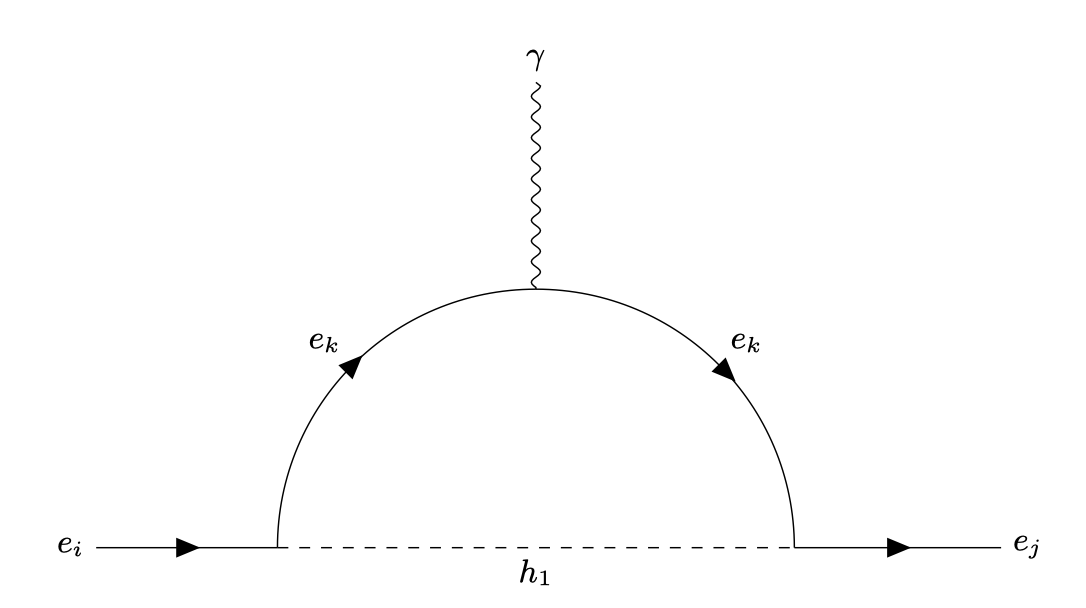
Figure 1: We denote an expression as $e_{i}e_{j},e_{k}$ where $e_{i}$, $e_{j}$ are the leptons in the outer legs and $e_{k}$ runs inside the loop. Similar diagrams with heavier scalars are also possible which are further suppressed by the large masses.

For $a_{\mu}$ calculation, the diagrams with muon inside the loop will dominate. The contribution of such diagrams to the muon anomalous magnetic moments is Leveille (1978)

$$\Delta a_{\mu\mu,\mu}=\left(y_{eh_{1}}\right)_{22}^{2}~{}\frac{m_{\mu}^{2}}{4\pi^{2}}~{}\int_{0}^{1}dx\frac{2x^{2}-x^{3}}{x^{2}m_{\mu}^{2}+(1-x)m_{h_{1}}^{2}}~{}.~{}\,$$ (70)

In Fig. 2, we show the allowed parameter space in the $(m_{h_{1}},(y_{eh_{1}})_{22})$ plane for $\Delta a_{\mu\mu,\mu}=\Delta a_{\mu}$. We also show relevant future bounds. This parameter space is allowed by all the muon experiment because $m_{h_{1}}<2m_{\mu}$.

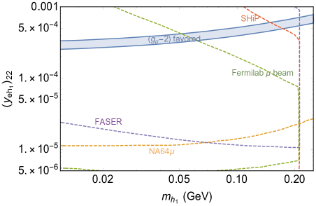
Figure 2: The blue shaded region shows the allowed parameter space favored by $\Delta a_{\mu}$. This region of the parameter space is allowed by all muon experiments. The dotted lines show the future bounds.

For the electron magnetic moment both tau and electron-induced loop diagrams are non-vanishing. The contributions to the electron anomalous magnetic moment with tau and electron inside the loop respectively are  Leveille (1978)

$$\Delta a_{ee,\tau} = \left(y_{eh_{1}}\right)_{13}\left(y_{eh_{1}}\right)_{31}~{}\frac{m_{e}^{2}}{4\pi^{2}}~{}$$ (71)

$$\times~{}\int_{0}^{1}dx\frac{x^{2}-x^{3}+\frac{m_{\tau}}{m_{e}}x^{2}}{x^{2}m_{e}^{2}+x(m_{\tau}^{2}-m_{e}^{2})+(1-x)m_{h_{1}}^{2}}~{},~{}\,$$

$$\Delta a_{ee,e}=\left(y_{eh_{1}}\right)_{11}^{2}~{}\frac{m_{e}^{2}}{4\pi^{2}}~{}\int_{0}^{1}dx\frac{2x^{2}-x^{3}}{x^{2}m_{e}^{2}+(1-x)m_{h_{1}}^{2}}~{}.~{}\,$$ (72)

Note that $\Delta a_{ee,e}$ always gives positive contributions while $\Delta a_{ee,\tau}$ can be negative if one of the couplings is negative. To explain the electron anomalous magnetic moment, we require that $\Delta a_{ee,\tau}$ gives the dominating contribution, and $\Delta a_{ee,\tau}+\Delta a_{ee,e}$ explains the deviation. In Fig. 3, we present various constraints mentioned in Sec. V in the $(m_{h_{1}},(y_{eh_{1}})_{11})$ plane. The values of $(y_{eh_{1}})_{13}$ and $(y_{eh_{1}})_{31}$ that gives, $\Delta a_{ee,\tau}\simeq\Delta a_{e}$ are shown in Eq. 73.

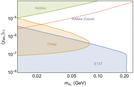
Figure 3: The shaded regions are the excluded regions and the dotted lines show the future bounds. The value of $(y_{eh_{1}})_{11})=10^{-5}$ chosen in Sec. V falls in the allowed region for $m_{h_{1}}=\mathcal{O}(100-200)$ MeV.

We choose one benchmark point which gives correct values and signs for both $\Delta a_{\mu}$ and $\Delta a_{e}$. The light scalar mass is $m_{h_{1}}=140$ MeV, and the elements of the Yukawa matrix $(y_{eh_{1}})_{ij}$ is given by

$$(y_{eh_{1}})_{ij}\simeq\left(\begin{array}[]{ccc}10^{-5}&0&-6.8\times 10^{-4}\\ 0&5.13\times 10^{-4}&10^{-7}\\ 3.5\times 10^{-4}&0&0\end{array}\right)~{}.~{}\,$$ (73)

In particular, these values do not vary much for the mass range $m_{h_{1}}=\mathcal{O}(100-200)$ MeV.

The Yukawa matrix in Eq. 73 introduces flavor violating decays mediating through the light scalar $h_{1}$: $\mu\rightarrow e\gamma$ with $\tau$ inside the loop,  $\tau\rightarrow e\gamma$ with $e$ inside the loop and $\tau\rightarrow\mu\gamma$ with $\mu$ inside the loop. The analytical expression of the branching fractions of these decays is given in Eq. 99. We show the values of these branching ratios using Eq. 73 and $m_{h_{1}}=140$ MeV and the corresponding experimental bounds Baldini et al. (2016); Aubert et al. (2010) in Table 4. We find that the branching ratios are smaller than the experimental bounds. The values do not change significantly over the mass range $m_{h_{1}}=\mathcal{O}(100-200)$ MeV.

Table 4: We summarize the values of different lepton flavor violating processes for the Yukawa matrix of Eq. 73. We also show corresponding experimental bounds.

Descriptions	Values for $m_{h_{1}}=140$ MeV	Experimental bounds
$\text{Br}(\mu\rightarrow e\gamma)$	$5.75\times 10^{-14}$	$<4.2\times 10^{-13}$
$\text{Br}(\tau\rightarrow e\gamma)$	$1.15\times 10^{-11}$	$<1.1\times 10^{-7}$
$\text{Br}(\tau\rightarrow\mu\gamma)$	$1.92\times 10^{-15}$	$<4.5\times 10^{-8}$

VII koto anomaly

The flavor changing processes like rare K meson decays, $K_{L}^{0}\rightarrow\pi^{0}\nu\bar{\nu}$ and $K^{+}\rightarrow\pi^{+}\nu\bar{\nu}$, are among the most sensitive probe for new physics beyond the SM Buras et al. (2015); Tanimoto and Yamamoto (2016); Crivellin et al. (2017); Bordone et al. (2017); Endo et al. (2018); He et al. (2018); Chen and Nomura (2018); Fajfer et al. (2018). These decays are loop suppressed in the SM Littenberg (1989); Cirigliano et al. (2012). Any observation of such a signal would require new physics for an explanation. The SM predictions are Buras et al. (2015)

$$\text{Br}(K_{L}^{0}\rightarrow\pi^{0}\nu\bar{\nu})_{\text{SM}} = (3.00\pm 0.30)\times 10^{-11}$$ (74)

$$\text{Br}(K^{+}\rightarrow\pi^{+}\nu\bar{\nu})_{\text{SM}} = (9.11\pm 0.72)\times 10^{-11}$$ (75)

The KOTO experiment Comfort et al. (2019); Yamanaka (2012) at J-PARC Nagamiya (2012) and NA62 experiment Cortina Gil et al. (2017) at CERN are dedicated to probing these processes. Recently, four candidate events were observed in the signal region of $K_{L}^{0}\rightarrow\pi^{0}\nu\bar{\nu}$ search at KOTO experiment, whereas the SM prediction is only $0.10\pm 0.02$ Shinohara (2019); Lin (2019). Out of four events, one can be suspected as a background coming from the SM upstream activity, while the other three can be considered as signals as they are not consistent with the currently known background. Given, single event sensitivity as $6.9\times 10^{-10}$ Shinohara (2019); Lin (2019), three events are consistent with

$$\text{Br}(K_{L}^{0}\rightarrow\pi^{0}\nu\bar{\nu})_{\text{_{\scriptsize{KOTO19}}}}<2.1^{+2.0(4.1)}_{-1.1(-1.7)}\times 10^{-9}$$ (76)

at 68(90)$\%$ C.L., including statistical uncertainties. The result includes the interpretation of photons and invisible final states as $\nu\bar{\nu}$. Note, the central value is almost two orders of magnitude larger than the SM prediction. This new result is in agreement with their previous bounds Ahn et al. (2019)

$$\text{Br}(K_{L}^{0}\rightarrow\pi^{0}\nu\bar{\nu})_{\text{_{\scriptsize{KOTO18}}}}<3.0\times 10^{-9}~{}.~{}\,$$ (77)

On the other hand, the charged kaon decay searches did not see any excess events. The recent update from NA62 puts a bound Ruggiero (2019)

$$\text{Br}(K^{+}\rightarrow\pi^{+}\nu\bar{\nu})_{\text{_{\scriptsize{NA62}}}}<2.44\times 10^{-10}$$ (78)

at 95$\%$ C.L., which is consistent with the SM prediction of Eq. 75.

In general, the neutral and charged kaon decays satisfy the following Grossman-Nir (GN) bound Grossman and Nir (1997)

$${\rm Br}\left(K^{0}_{L}\rightarrow\pi^{0}\nu{\bar{\nu}}\right)\leq 4.3\times{\rm Br}\left(K^{+}\rightarrow\pi^{+}\nu{\bar{\nu}}\right)~{},~{}\,$$ (79)

which depends on the isospin symmetry and kaon lifetimes. The GN bound might give a strong constraint on the explanations for the KOTO anomaly. Thus, the new physics explanation for the KOTO anomaly is required to generate three anomalous events and satisfy the GN bound. Several such solutions have been proposed in the literature Kitahara et al. (2020); Fabbrichesi and Gabrielli (2020); Egana-Ugrinovic et al. (2020); Dev et al. (2020); Li et al. (2020); Jho et al. (2020); Liu et al. (2020); Liao et al. (2020); Cline et al. (2020); Gori et al. (2020); He et al. (2020a, b); Datta et al. (2020); Foroughi-Abari and Ritz (2020); Altmannshofer et al. (2020).

In this work, we rely on the tree-level flavor violating couplings of the light scalar $h_{1}$ in the quark sector of Eq. 45 and invisible decay channel of $h_{1}$ to interpret Eq. 76. The non-zero value of $(y_{dh_{1}})_{21}$ leads to the tree-level $s\rightarrow d$ transition through $h_{1}$. Thus, the neutral kaon can decay into a neutral pion and a $h_{1}$ through the tree-level coupling. The same coupling would allow the charged kaon to decay into a charged pion and a $h_{1}$. The produced $h_{1}$ promptly decays into either a DM pair $n_{1}\bar{n}_{1}$ or an electron pair. The decay channel $\text{Br}(K_{L}^{0}\rightarrow\pi^{0}n_{1}\bar{n}_{1})$ will mimic the $\text{Br}(K_{L}^{0}\rightarrow\pi^{0}\nu\bar{\nu})$ search signals and can account for the required branching fractions of Eq. 76. Note that the $\text{Br}(K^{+}\rightarrow\pi^{+}+\text{invisible})$ bound is generally stronger except in the mass range $\sim m_{\pi}\pm 25$ MeV Ruggiero (2019); Artamonov et al. (2009); Cortina Gil et al. (2019); Fuyuto et al. (2015), therefore, we choose the mass parameter $m_{h_{1}}$ in that range to evade the GN bound,

The non-zero coupling $(y_{dh_{1}})_{21}$ also gives the tree-level $K^{0}-\bar{K}^{0}$ mixing mediated via $h_{1}$. The contribution of this mixing to the $K_{L}-K_{S}$ mass difference can be calculated as follows

$$\Delta m_{K}=-\frac{2(y_{dh_{1}})_{21}^{2}}{m_{h_{1}}^{2}}\frac{f_{K}^{2}m_{K}^{2}}{12m_{K}}\left[1-\frac{m_{K}^{2}}{(m_{s}+m_{d})^{2}}\right]~{},~{}\,$$ (80)

with $\Delta m_{K}^{\text{exp}}=3.52\times 10^{-15}$ GeV Tanabashi et al. (2018). Here. $f_{K}\simeq 1.23m_{\pi}$ is the kaon decay constant Tanabashi et al. (2018). For $m_{h_{1}}=\mathcal{O}(100-200)$ MeV, one only needs $(y_{dh_{1}})_{21}<10^{-8}$ to avoid this constraint, which is obviously satisfied in the following discussions.

The decay width of $K_{L}^{0}$ decaying into a neutral pion and an on-shell $h_{1}$ is

$$\Gamma(K_{L}^{0}\rightarrow\pi^{0}h_{1}) = \frac{[{\rm Re}(y_{dh_{1}})_{21}]^{2}}{16\pi m_{K_{L}^{0}}}~{}\left(\frac{m_{K^{0}}^{2}-m_{\pi^{0}}^{2}}{m_{s}-m_{d}}\right)^{2}f^{2}(m_{h_{1}}^{2})$$ (81)

$$\times~{}\lambda^{1/2}\left(1,\frac{m_{\pi^{0}}^{2}}{m_{K_{L}^{0}}^{2}},\frac{m_{h_{1}}^{2}}{m_{K_{L}^{0}}^{2}}\right)~{},~{}\,$$

where $\lambda(x,y,z)=x^{2}+y^{2}+z^{2}-2xy-2yz-2zx$ is the triangle function, and the function $f(q^{2})$ for the vector form factor is defined as McWilliams and Shanker (1980)

$$f(q^{2}) = f_{+}(0)\left(1+\frac{\lambda_{0}}{m_{\pi}^{2}}q^{2}\right)$$ (82)

with $f_{+}(0)=0.97$ and $\lambda_{0}=1.8\times 10^{-2}$.

And the decay width of $K_{L}^{+}$ decaying into a charged pion and an on-shell $h_{1}$ is

$$\Gamma(K^{\pm}\rightarrow\pi^{\pm}h_{1}) = \frac{|(y_{dh_{1}})_{21}|^{2}}{16\pi m_{K^{\pm}}}~{}\left(\frac{m_{K^{\pm}}^{2}-m_{\pi^{\pm}}^{2}}{m_{s}-m_{d}}\right)^{2}f^{2}(m_{h_{1}}^{2})$$ (83)

$$\times~{}\lambda^{1/2}\left(1,\frac{m_{\pi^{\pm}}^{2}}{m_{K^{\pm}}^{2}},\frac{m_{h_{1}}^{2}}{m_{K^{\pm}}^{2}}\right)~{}.~{}\,$$

The $h_{1}$ produced in the decay of the kaon is short-lived with typical lifetime $\tau_{h_{1}}\simeq 10^{-13}$ sec for the choice of the parameters in Sec. V. Now taking the energy of the produced $h_{1}$ to be $E_{h_{1}}\simeq 1.5$ GeV, we estimate the path it travels before it decays as, $\gamma c\tau_{h_{1}}\simeq 10^{-4}$ m. The length of the KOTO detector is $3$ m, hence $h_{1}$ decays inside the detector. It can promptly decay into $n_{1}\bar{n}_{1}$ or $e^{+}e^{-}$ pair with branching fractions of $0.95$ and $0.05$, respectively. So we get

$$\text{Br}(K_{L}^{0}\rightarrow\pi^{0}n_{1}\bar{n}_{1}) = \frac{\Gamma(K_{L}^{0}\rightarrow\pi^{0}h_{1})\times\text{Br}(h_{1}\rightarrow n_{1}\bar{n}_{1})}{\Gamma_{K_{L}^{0}}},$$

$$\text{Br}(K_{L}^{0}\rightarrow\pi^{0}e^{+}e^{-}) = \frac{\Gamma(K_{L}^{0}\rightarrow\pi^{0}h_{1})\times\text{Br}(h_{1}\rightarrow e^{+}e^{-})}{\Gamma_{K_{L}^{0}}},$$

where $\Gamma_{K_{L}^{0}}=\Gamma_{K_{L}^{0}}^{\text{SM}}+\Gamma(K_{L}^{0}\rightarrow\pi^{0}n_{1}\bar{n}_{1})+\Gamma(K_{L}^{0}\rightarrow\pi^{0}e^{+}e^{-})$ with $\Gamma_{K_{L}^{0}}^{\text{SM}}=(1.29\pm 0.01)\times 10^{-17}$ GeV. We get similar expressions for the $K^{\pm}$ decays.

In Fig. 4, we show the favored parameter space in $(m_{h_{1}},(y_{dh_{1}})_{21})$ plane corresponding to the branching fraction of Eq. 76. We also show the region excluded by KOTO 2018 result and $K_{L}^{0}\rightarrow\pi^{0}e^{+}e^{-}$ decay channel. As mentioned earlier, the KOTO favored region is allowed by the NA62 experiment, thus avoiding the GN bound.

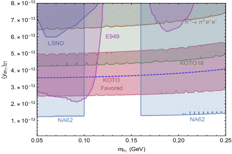
Figure 4: The pink shaded region is the parameter space favored by the KOTO anomaly in our model. The blue dashed line is the contour corresponding to the central value of the KOTO anomaly. The green contour corresponds to the KOTO18 excluded region. Contour line corresponding to the $K_{L}^{0}\rightarrow\pi^{0}e^{+}e^{-}$ decay is shown in brown. We also show the excluded region by NA62, E949 and LSND.

VIII Miniboone excess

MiniBooNE is a Cherenkov detector consists of a $12.2$ m diameter sphere filled with 818 tonnes of pure mineral oil (CH₂), located at the Booster Neutrino Beam (BNB) line at Fermilab Aguilar-Arevalo et al. (2009a). The experiment gets the neutrinos and antineutrinos flux from BNB Aguilar-Arevalo et al. (2009b). Recently, in 2018, after taking data for 15 years, they have reported a $4.7\sigma$ excess of $\nu_{e}+\bar{\nu}_{e}$ like events over the estimated background in the energy range $200<E_{\nu}^{QE}<1250$ MeV  Aguilar-Arevalo et al. (2018). The amount of combined excess events is $460.5\pm 99.0$ corresponding to $12.84\times 10^{20}$ protons on target in neutrino mode and $11.27\times 10^{20}$ protons on target in antineutrino mode. This result is in tension with the two-neutrino oscillation within the standard three neutrino scenario. More recently this result was updated by MiniBooNE with $638\pm 132.8$ electron-like events (4.8$\sigma$) as the reported number of excess events corresponding to $18.75\times 10^{20}$ protons on target in neutrino mode and $11.27\times 10^{20}$ protons on target in antineutrino mode Aguilar-Arevalo et al. (2020).

Recently, several attempts have been put forth to explain this anomaly within the context of dark neutrino mass models using heavy sterile neutrinos and dark gauge bosons Bertuzzo et al. (2019, 2018); Ballett et al. (2019a, b, 2020); Abdallah et al. (2020) and dark sector models with dark scalars Datta et al. (2020). They all considered the scenario where the light neutrinos upscatter to a heavy neutrino after coherent scattering off the nucleus and subsequent decay of the heavy neutrino into a pair of electrons. The MiniBooNE detector cannot distinguish the electron pair. One can get the reconstructed neutrino energy using the energy and angular distribution of the mediator coming from the sterile neutrino decay Martini et al. (2012). Recently, it was shown that parameter space needed for the explanation of MiniBooNE data in the dark gauge boson models are constrained by CHARM-II data Argüelles et al. (2019), because the scattering cross-section get enhanced for large neutrino energy. The scalar mediator models have the advantages as for similar parameters, as the scattering cross-section is much smaller Datta et al. (2020).

In the framework of our model, the heavy sterile neutrino $n_{2}$ can be produced from the upscattering process: $\nu_{2}A\rightarrow n_{2}A$ mediated through the light scalar $h_{1}$ as shown Fig. 5. The $\nu_{2}A$ scattering being coherent is enhanced by $\sim A^{2}$. The produced $n_{2}$ promptly decays into $n_{1}$ and an on-shell $h_{1}$, which subsequently decays into a pair of $e^{+}e^{-}$ with $\text{Br}(h_{1})\rightarrow e^{+}e^{-}\simeq 5\%$. Taking the typical energies, $E_{n_{2}},E_{h_{1}}\sim 1$ GeV, we estimate the length of the path they travel before decay as $l_{n_{2}}\leq 10^{-4}$ m and $l_{h_{1}}\simeq 10^{-4}$ m.

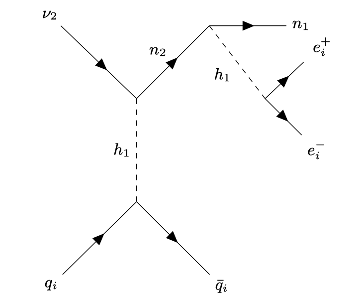
Figure 5: The Feynman diagram for the upscattering process $\nu A\rightarrow nA$ that contributes to the cross-section that generates the MiniBooNE excess events in our model.

As both the heavy neutrino $n_{2}$ and the light scalar $h_{1}$ decay promptly, we can write the total number of events observed due to this process as

$$N_{\text{event}} = f_{\text{exp}}\int_{E_{\nu_{\text{min}}}}^{E_{\nu_{\text{max}}}}dE_{\nu}\Phi(E_{\nu})\int_{E_{R_{\text{min}}}}^{E_{R_{\text{max}}}}dE_{R}$$ (85)

$$\times~{}\frac{d\sigma(E_{R},E_{\nu})}{dE_{R}}\times\text{Br}(h_{1}\rightarrow e^{+}e^{-})~{},~{}\,$$

where $f_{\text{exp}}$ is a factor which involves the numbers of protons on target, exposure, effective area of the detector and depends on the experiments; $E_{R}$ is the nuclear recoil energy; $E_{\nu}$ is the incoming neutrino energy; and $\Phi(E_{\nu})$ is the incoming neutrino flux from the BNB. Therefore, $f_{\text{model}}=N_{\text{event}}/f_{\text{exp}}$ is the model-dependent part.

The differential scattering cross-section of $\nu A\rightarrow nA$ is given by

$$\frac{d\sigma}{dE_{R}} = [Zf_{p}+(A-Z)f_{n}]^{2}\frac{(y_{nh_{1}})_{22}^{2}}{16\pi E_{\nu}^{2}}$$ (86)

$$\times \frac{(m_{n_{2}}^{2}+2m_{A}E_{R})(2m_{A}+E_{R})}{(m_{h_{1}}^{2}+2m_{A}E_{R})^{2}}F^{2}(E_{R})~{},~{}\,$$

where $m_{A}$ is the mass of the target nucleus; $Z$ and $A-Z$ are the proton and neutron numbers of the target nucleus; $F(E_{R})$ is the nuclear form factor Helm (1956); Engel (1991); and the factors $f_{p,n}$ are defined as Falk et al. (2000)

$$\frac{f_{p,n}}{m_{N}}=\sum_{q=u,d,s}f_{T_{q}}^{(p,n)}\frac{f_{q}}{m_{q}}+\frac{2}{27}\left(1-\sum_{q=u,d,s}f_{T_{q}}^{(p,n)}\right)\sum_{q=c,b,t}\frac{f_{q}}{m_{q}}.$$ (87)

We take, $f_{(u,d)}=(y_{(u,d)h_{1}})_{11}$ and $f_{s,c,b,t}=0$. The constants $f_{T_{u}}^{(p)}$, $f_{T_{d}}^{(p)},f_{T_{u}}^{(n)}$ and $f_{T_{d}}^{(n)}$ are taken to have the values 0.020, 0.041, 0.0189, and 0.0451, respectively Alarcon et al. (2012, 2014); Crivellin et al. (2014); Hoferichter et al. (2015); Junnarkar and Walker-Loud (2013).

Fig. 6 shows the allowed values of $n_{2}$ masses for $m_{h_{1}}=\mathcal{O}(100-200)$ MeV to generate the MiniBooNE events given the couplings : $(y_{nh_{1}})_{22}=6.1\times 10^{-2}$, $(y_{uh_{1}})_{11}=5.0\times 10^{-6}$ and $(y_{dh_{1}})_{11}=5.0\times 10^{-6}$. This is consistent with the neutrino masses and mixing in our model as shown in Table. 1.

Figure 6: The shaded region is the allowed parameter space in the $(m_{h_{1}},m_{n_{2}})$ plane which gives the desired numbers of total events. We take the couplings: $(y_{nh_{1}})_{22}=6.1\times 10^{-2}$, $(y_{uh_{1}})_{11}=5.0\times 10^{-6}$ and $(y_{dh_{1}})_{11}=5.0\times 10^{-6}$.

We choose one typical benchmark point $m_{n_{2}}=420~{}\text{MeV and }~{}m_{h_{1}}=140~{}\text{MeV}$ to show the scattering cross-section as a function of the incoming neutrino energy in Fig. 7. Note, the cross-section is small at the relevant incoming neutrino energy, $E_{\nu_{\mu}}=20$ GeV Layda (1991) of the CHARM-II experiment De Winter et al. (1989); Geiregat et al. (1993); Vilain et al. (1994), therefore gives no excess events Datta et al. (2020). It was shown recently Brdar et al. (2020) that, if the decay length of the produced sterile neutrino $n_{2}$ in the upscattering has decay length $l_{n_{2}}\leq 10^{-4}$ m, then the scalar mediated process does not produce any excess events in T2K ND280 Abe et al. (2011); Kudenko (2009); Assylbekov et al. (2012); Amaudruz et al. (2012); Abe et al. (2013, 2019) and MINER$\nu$A Wolcott et al. (2016a); Park et al. (2016); Wolcott et al. (2016b); Valencia et al. (2019) experiments. We also verify that our model-dependent part $f_{\text{model}}$ is consistent with other dark gauge bosons Bertuzzo et al. (2018); Argüelles et al. (2019) or dark scalar models Datta et al. (2020). We show the estimated number of excess events for a few benchmark points in Table 6.

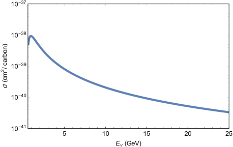
Figure 7: The line shows the cross section as a function of the incoming neutrino energy for the BP: $m_{n_{2}}=420~{}\text{MeV}$, $m_{h_{1}}=140~{}\text{MeV}$, $(y_{nh_{1}})_{22}=6.1\times 10^{-2}$, $(y_{uh_{1}})_{11}=5.0\times 10^{-6}$, and $(y_{dh_{1}})_{11}=5.0\times 10^{-6}$.

IX discussions

We have considered a general framework of the scalar singlet-doublet extension of the SM scalar sector and added three sterile neutrinos. We have generated a very interesting physical particle mass spectrum which has rich phenomenological consequences. In particular, the particles that play central role in our analysis are: one light scalar with mass $m_{h_{1}}\sim\mathcal{O}(100-200)$ MeV, the lightest sterile neutrino with mass $m_{n_{1}}\sim\mathcal{O}(1-10)$ keV and the next-to-lightest sterile neutrino with mass $m_{n_{2}}\sim\mathcal{O}(400)$ MeV. The lightest sterile neutrino $n_{1}$ can be a viable DM candidate. $n_{1}$ with a mass of 7 keV can explain the 3.5 keV line in the X-ray search. We have shown that one can get tiny neutrino mass and DM relic abundance in this model as well.

The main focus of the work was to address a few of the recent experimental puzzles: anomalous magnetic moments of both muon and electron; KOTO anomalous events and excess events found in the MiniBooNE neutrino experiment. The tree-level flavor violating couplings of the light scalar to the leptons enable us to explain the $(g-2)_{\mu,e}$ using one-loop diagrams. And the flavor violation in the quark sector allows the Kaon to decay at tree level. All the flavor violations associated with the scalars in this model appear at the tree level. The MiniBooNE, on the other hand, requires the production of heavy sterile neutrino from the light scalar mediated neutrino-nucleus scattering. Note, the tree-level FCNC of the light scalar and the decay of the light scalar to electron-positron pair and a pair of lightest sterile neutrinos connect all three puzzles.

Table 5: Three BPs are shown, for which we calculate the different observables quantities, and can account for three anomalies.

Parameters	BP1	BP2	BP3
$m_{h_{1}}(\text{MeV})$	$130$	$140$	$150$
$m_{n_{1}}(\text{keV})$	$2$	$3$	$2$
$m_{n_{2}}(\text{MeV})$	$435$	$420$	$440$
$(y_{eh_{1}})_{22}$	$5\times 10^{-4}$	$4.75\times 10^{-4}$	$5.5\times 10^{-4}$
$(y_{eh_{1}})_{13}$	$-3.5\times 10^{-4}$	$-6\times 10^{-4}$	$-6.8\times 10^{-4}$
$(y_{eh_{1}})_{31}$	$6.8\times 10^{-4}$	$4\times 10^{-4}$	$3.5\times 10^{-4}$
$(y_{dh_{1}})_{21}$	$3\times 10^{-13}$	$3.5\times 10^{-13}$	$4\times 10^{-13}$

We showed that the parameter space found in Sec. III-V can explain these anomalies simultaneously. We found that the light scalar mass is tightly constrained for the explanation of the KOTO anomaly which emerges in a large region in the allowed parameter space. We chose three BPs in the allowed region of the parameter space and summarize them in Table 5. For all these BPs, we fix the coupling constants: $(y_{nnh_{1}})_{11}=7\times 10^{-5}$, $(y_{eh_{1}})_{11}=1\times 10^{-5}$, $(y_{nh_{1}})_{22}=6.1\times 10^{-2}$, $(y_{uh_{1}})_{11}=5.0\times 10^{-6}$, and $(y_{dh_{1}})_{11}=5.0\times 10^{-6}$. We summarize the observables in Table 6. These BPs can also explain neutrino masses and mixing angles.

Table 6: The observables corresponding to the three BPs.

Observables	BP1	BP2	BP3
$\Omega_{n_{1}}h^{2}$	$0.1$	$0.1$	$0.1$
$\Delta a_{\mu}\times 10^{-9}$	$2.67$	$2.27$	$2.86$
$\Delta a_{e}\times 10^{-13}$	$-8.43$	$-8.50$	$-8.43$
$Br(K_{L}^{0}\rightarrow\pi^{0}n_{1}\bar{n}_{1})\times 10^{-9}~{}$	$1.42$	$1.91$	$2.47$
$Br(K_{L}^{0}\rightarrow\pi^{0}e^{+}e^{-})\times 10^{-11}~{}$	$5.81$	$7.82$	$1.01$
$N_{\text{event}}~{}(\nu+\bar{\nu})$	$671$	$644$	$497$

The parameter space associated with the explanation of MiniBooNE excess is not constrained by the existing data from MINER$\nu$A, CHARM-II and T2K ND280 data due to the scalar mediator. If however, in future, the MiniBooNE data requires the scalar mediator mass to be $\leq 100$ MeV then the KOTO explanation would be in tension with the model. In that case, we would need more than one light scalar to satisfy both KOTO and MiniBooNE anomalies. Further, since this model has three sterile neutrinos, the lightest sterile neutrino mass can be $\sim 1$ eV which satisfies the oscillation data whereas the second to lightest neutrino ($\sim 400$ MeV) can explain the low energy excess in the MiniBooNE data.

The light scalar model we presented in this paper appears to be quite effective in explaining the DM content, neutrino masses, and various anomalies. This model would be investigated as we obtain more results on these anomalies from KOTO, $(g-2)_{\mu,e}$, MicroBooNE etc. along with various ongoing and upcoming experiments, e.g., NA64$\mu$,e; FASER, SHiP, Fermilab $\mu$-beam etc. and various lepton flavor violating rare decays.

Appendix A Higgs Basis Transformation

We consider two complex scalar doublet $H_{1,2}$ and one scalar singlet $H_{S}$ singlet with the following quantum numbers under $SU(2)_{L}\times U(1)_{Y}$ gauge symmetry

$$H_{1}\sim(2,1/2),~{}~{}~{}~{}~{}H_{2}\sim(2,1/2),~{}~{}~{}~{}~{}H_{S}\sim(1,0)~{}.~{}\,$$ (88)

The most general charge conserving vev’s are

$$\small{\braket{H_{1}}=\left(\begin{array}[]{c}0\\ \frac{v_{1}}{\sqrt{2}}\end{array}\right),~{}\braket{H_{2}}=\left(\begin{array}[]{c}0\\ \frac{v_{2}}{\sqrt{2}}\end{array}\right),~{}\braket{H_{S}}=\frac{v_{3}}{\sqrt{2}}}~{}.~{}\,$$ (93)

We redefine the neutral components of the Higgs fields by rotating via a Unitary matrix $U$ in such a way that only one scalar doublet will develop a non-zero vev. The neutral components of the new Higgs fields can be written as

$$\phi^{0}_{a}=\sum_{b}U_{ab}H^{0}_{b}~{},~{}\,$$ (94)

where, $a,b=1,2$ and $S$. The Unitary matrix $U$ is given as

$$U=\left(\begin{array}[]{ccc}\frac{v_{1}}{v}&\frac{v_{2}}{v}&\frac{v_{3}}{v}\\ -\frac{v_{2}}{v}&\frac{v_{1}}{v}&0\\ -\frac{v_{3}}{v}&0&\frac{v_{1}}{v}\end{array}\right)~{}.~{}\,$$ (95)

It is easy to see that the vev’s of the new Higgs fields are given by

$$\braket{\phi^{0}_{1}}=\left(\begin{array}[]{c}0\\ \frac{v}{\sqrt{2}}\end{array}\right),~{}\braket{\phi^{0}_{2}}=0,~{}\braket{\phi^{0}_{S}}=0~{},~{}\,$$ (96)

where $v=\left(v_{1}^{2}+v_{2}^{2}+v_{3}^{2}\right)^{1/2}$. Therefore, only one doublet will control the spontaneous electroweak gauge symmetry breaking and the generation of the SM fermion masses.

Appendix B Numerical Calculation of Scalar Spectrum

Some details about the numerical analysis of Sec. V is given here. Given the benchmark values of the parameters in Table 2, one can follow Eqs. 11-II to calculate the mixing of the scalar interaction states and the masses of the physical scalars. The summary of the masses is given in Table 3. In particular, the physical neutral scalars are given by $h_{i}=(U_{R}^{-1})_{ij}\rho_{j}$:

$$h_{2} = 0.056~{}\rho_{1}+0.995~{}\rho_{2}+0.081~{}\rho_{3}~{},~{}\,$$

$$h = 0.997~{}\rho_{1}-0.053~{}\rho_{2}-0.035~{}\rho_{3}~{},~{}\,$$

$$h_{1} = 0.030~{}\rho_{1}-0.083~{}\rho_{2}+0.996~{}\rho_{3}~{}.~{}\,$$ (97)

Eq. B tells us that the heavy scalar $h_{2}$ mostly comes from the second doublet $\phi_{2}$, while the SM Higgs is associated with the doublet $\phi_{1}$. The light scalar $h_{1}$ mostly comes from the singlet. These mixing elements also enter into Eq. II. The mixing angle between the pseudoscalars are $\alpha=5.44^{\degree}$ and the physical states are given by

$$s_{1} = 0.995~{}\eta_{2}-0.094~{}\eta_{S}~{},~{}\,$$

$$s_{2} = 0.094~{}\eta_{2}+0.995~{}\eta_{S}~{}.~{}\,$$ (98)

The physical scalars $s_{1}$ and $s_{2}$ are mostly associated with the doublet $\phi_{2}$ and $\phi_{S}$, respectively.

Appendix C Calculation of $e_{i}\rightarrow e_{j}\gamma$

The most general expression for the branching fraction of the process $e_{i}\rightarrow e_{j}\gamma$ for a light scalar mediator of Fig. 1 is given by

$$\text{Br}(e_{i}\rightarrow e_{j}\gamma) = \frac{\Gamma(e_{i}\rightarrow e_{j}\gamma)}{\Gamma(e_{i}\rightarrow e_{j}\bar{\nu}_{j}\nu_{i})}$$ (99)

$$= \frac{3\alpha}{8\pi G_{F}^{2}m_{e_{i}}^{2}}\left(1-\frac{m_{e_{j}}^{2}}{m_{e_{i}}^{2}}\right)\left[(y_{eh_{1}})_{ik}(y_{eh_{1}})_{kj}\right]^{2}$$

$$\times~{}\frac{I_{1}(m_{e_{i}},m_{e_{j}},m_{e_{k}},m_{h_{1}})}{I_{2}(m_{e_{j}}^{2}/m_{e_{i}}^{2})}~{},~{}\,$$

where the lepton $e_{k}$ runs inside the loop. The function $I_{1}(m_{e_{i}},m_{e_{j}},m_{e_{k}},m_{h_{1}})$ comes from the partial decay width $\Gamma(e_{i}\rightarrow e_{j}\gamma)$ whereas $I_{2}(m_{e_{j}}^{2}/m_{e_{i}}^{2})$ comes from $\Gamma(e_{i}\rightarrow e_{j}\bar{\nu}_{j}\nu_{i})$ . The definitions of the functions $I_{1}$ and $I_{2}$ respectively are

$$I_{1}(m_{e_{i}},m_{e_{j}},m_{e_{k}},m_{h_{1}})=\int_{0}^{1}dz\int_{0}^{1-z}dy$$ (100)

$$~{}~{}~{}~{}~{}\times\frac{yz(m_{e_{j}}-m_{e_{i}})-(z-1)(zm_{e_{i}}+m_{e_{k}})}{z(y+z-1)m_{e_{i}}^{2}-yzm_{e_{j}}^{2}+(1-z)m_{e_{k}}^{2}+zm_{h_{1}}^{2}}~{},~{}\,$$

$$I_{2}\left(\frac{m_{e_{j}}^{2}}{m_{e_{i}}^{2}}\right)=1-8\frac{m_{e_{j}}^{2}}{m_{e_{i}}^{2}}+8\frac{m_{e_{j}}^{6}}{m_{e_{i}}^{6}}-\frac{m_{e_{j}}^{8}}{m_{e_{i}}^{8}}$$

$$~{}~{}~{}~{}~{}~{}~{}~{}~{}~{}~{}~{}~{}~{}~{}~{}~{}+12\frac{m_{e_{j}}^{4}}{m_{e_{i}}^{4}}\ln\left(\frac{m_{e_{i}}^{2}}{m_{e_{j}}^{2}}\right)~{}.~{}\,$$

References

- Fukuda et al. (1998) Y. Fukuda et al. (Super-Kamiokande), Phys. Rev. Lett. 81, 1562 (1998), arXiv:hep-ex/9807003 [hep-ex] .
- Ahmad et al. (2002) Q. R. Ahmad et al. (SNO), Phys. Rev. Lett. 89, 011301 (2002), arXiv:nucl-ex/0204008 [nucl-ex] .
- Aghanim et al. (2018) N. Aghanim et al. (Planck), (2018), arXiv:1807.06209 [astro-ph.CO] .
- Bennett et al. (2006) G. W. Bennett et al. (Muon g-2), Phys. Rev. D73, 072003 (2006), arXiv:hep-ex/0602035 [hep-ex] .
- Tanabashi et al. (2018) M. Tanabashi et al. (Particle Data Group), Phys. Rev. D98, 030001 (2018).
- Davier et al. (2017) M. Davier, A. Hoecker, B. Malaescu, and Z. Zhang, Eur. Phys. J. C77, 827 (2017), arXiv:1706.09436 [hep-ph] .
- Blum et al. (2018) T. Blum, P. A. Boyle, V. Gülpers, T. Izubuchi, L. Jin, C. Jung, A. Jüttner, C. Lehner, A. Portelli, and J. T. Tsang (RBC, UKQCD), Phys. Rev. Lett. 121, 022003 (2018), arXiv:1801.07224 [hep-lat] .
- Keshavarzi et al. (2018) A. Keshavarzi, D. Nomura, and T. Teubner, Phys. Rev. D97, 114025 (2018), arXiv:1802.02995 [hep-ph] .
- Davier et al. (2020) M. Davier, A. Hoecker, B. Malaescu, and Z. Zhang, Eur. Phys. J. C 80, 241 (2020), [Erratum: Eur.Phys.J.C 80, 410 (2020)], arXiv:1908.00921 [hep-ph] .
- Hanneke et al. (2011) D. Hanneke, S. F. Hoogerheide, and G. Gabrielse, Phys. Rev. A83, 052122 (2011), arXiv:1009.4831 [physics.atom-ph] .
- Hanneke et al. (2008) D. Hanneke, S. Fogwell, and G. Gabrielse, Phys. Rev. Lett. 100, 120801 (2008), arXiv:0801.1134 [physics.atom-ph] .
- Aoyama et al. (2018) T. Aoyama, T. Kinoshita, and M. Nio, Phys. Rev. D97, 036001 (2018), arXiv:1712.06060 [hep-ph] .
- Parker et al. (2018) R. H. Parker, C. Yu, W. Zhong, B. Estey, and H. Müller, Science 360, 191 (2018), arXiv:1812.04130 [physics.atom-ph] .
- Hiller et al. (2019) G. Hiller, C. Hormigos-Feliu, D. F. Litim, and T. Steudtner, (2019), arXiv:1910.14062 [hep-ph] .
- Blum et al. (2020) T. Blum, N. Christ, M. Hayakawa, T. Izubuchi, L. Jin, C. Jung, and C. Lehner, Phys. Rev. Lett. 124, 132002 (2020), arXiv:1911.08123 [hep-lat] .
- Campanario et al. (2019) F. Campanario, H. Czyż, J. Gluza, T. Jeliński, G. Rodrigo, S. Tracz, and D. Zhuridov, Phys. Rev. D 100, 076004 (2019), arXiv:1903.10197 [hep-ph] .
- Shinohara (2019) S. Shinohara, Search for the rare decay at JPARC KOTO experiment (2019), KAON2019, Perugia, Italy.
- Lin (2019) C. Lin, Recent Result on the Measurement of at the J-PARC KOTO Experiment (2019), J-PARC Symposium.
- Buras et al. (2015) A. J. Buras, D. Buttazzo, J. Girrbach-Noe, and R. Knegjens, JHEP 11, 033 (2015), arXiv:1503.02693 [hep-ph] .
- Ruggiero (2019) G. Ruggiero, New Result on from the NA62 Experiment (2019), KAON2019, Perugia, Italy.
- Artamonov et al. (2009) A. Artamonov et al. (BNL-E949), Phys. Rev. D 79, 092004 (2009), arXiv:0903.0030 [hep-ex] .
- Branco et al. (2012) G. Branco, P. Ferreira, L. Lavoura, M. Rebelo, M. Sher, and J. P. Silva, Phys. Rept. 516, 1 (2012), arXiv:1106.0034 [hep-ph] .
- Aguilar-Arevalo et al. (2018) A. Aguilar-Arevalo et al. (MiniBooNE), Phys. Rev. Lett. 121, 221801 (2018), arXiv:1805.12028 [hep-ex] .
- Aguilar-Arevalo et al. (2020) A. Aguilar-Arevalo et al. (MiniBooNE), (2020), arXiv:2006.16883 [hep-ex] .
- Higgs (1964) P. W. Higgs, Phys. Rev. Lett. 13, 508 (1964).
- Higgs (1966) P. W. Higgs, Phys. Rev. 145, 1156 (1966).
- Englert and Brout (1964) F. Englert and R. Brout, Phys. Rev. Lett. 13, 321 (1964).
- Guralnik et al. (1964) G. Guralnik, C. Hagen, and T. Kibble, Phys. Rev. Lett. 13, 585 (1964).
- Kibble (1967) T. Kibble, Phys. Rev. 155, 1554 (1967).
- Lee (1973) T. Lee, Phys. Rev. D 8, 1226 (1973).
- He et al. (2009) X.-G. He, T. Li, X.-Q. Li, J. Tandean, and H.-C. Tsai, Phys. Rev. D 79, 023521 (2009), arXiv:0811.0658 [hep-ph] .
- Grzadkowski and Osland (2010) B. Grzadkowski and P. Osland, Phys. Rev. D 82, 125026 (2010), arXiv:0910.4068 [hep-ph] .
- Logan (2011) H. E. Logan, Phys. Rev. D 83, 035022 (2011), arXiv:1010.4214 [hep-ph] .
- Boucenna and Profumo (2011) M. Boucenna and S. Profumo, Phys. Rev. D 84, 055011 (2011), arXiv:1106.3368 [hep-ph] .
- He et al. (2012) X.-G. He, B. Ren, and J. Tandean, Phys. Rev. D 85, 093019 (2012), arXiv:1112.6364 [hep-ph] .
- Bai et al. (2013) Y. Bai, V. Barger, L. L. Everett, and G. Shaughnessy, Phys. Rev. D 88, 015008 (2013), arXiv:1212.5604 [hep-ph] .
- He and Tandean (2013) X.-G. He and J. Tandean, Phys. Rev. D 88, 013020 (2013), arXiv:1304.6058 [hep-ph] .
- Cai and Li (2013) Y. Cai and T. Li, Phys. Rev. D 88, 115004 (2013), arXiv:1308.5346 [hep-ph] .
- Guo and Kang (2015) J. Guo and Z. Kang, Nucl. Phys. B 898, 415 (2015), arXiv:1401.5609 [hep-ph] .
- Wang and Han (2014) L. Wang and X.-F. Han, Phys. Lett. B 739, 416 (2014), arXiv:1406.3598 [hep-ph] .
- Drozd et al. (2014) A. Drozd, B. Grzadkowski, J. F. Gunion, and Y. Jiang, JHEP 11, 105 (2014), arXiv:1408.2106 [hep-ph] .
- Campbell et al. (2015) R. Campbell, S. Godfrey, H. E. Logan, A. D. Peterson, and A. Poulin, Phys. Rev. D 92, 055031 (2015), [Erratum: Phys.Rev.D 101, 039905 (2020)], arXiv:1505.01793 [hep-ph] .
- Drozd et al. (2016) A. Drozd, B. Grzadkowski, J. F. Gunion, and Y. Jiang, JCAP 10, 040 (2016), arXiv:1510.07053 [hep-ph] .
- von Buddenbrock et al. (2016) S. von Buddenbrock, N. Chakrabarty, A. S. Cornell, D. Kar, M. Kumar, T. Mandal, B. Mellado, B. Mukhopadhyaya, R. G. Reed, and X. Ruan, Eur. Phys. J. C 76, 580 (2016), arXiv:1606.01674 [hep-ph] .
- Muhlleitner et al. (2017) M. Muhlleitner, M. O. P. Sampaio, R. Santos, and J. Wittbrodt, JHEP 03, 094 (2017), arXiv:1612.01309 [hep-ph] .
- Liu et al. (2016) X. Liu, L. Bian, X.-Q. Li, and J. Shu, Nucl. Phys. B 909, 507 (2016), arXiv:1508.05716 [hep-ph] .
- Georgi and Nanopoulos (1979) H. Georgi and D. V. Nanopoulos, Phys. Lett. B 82, 95 (1979).
- Botella and Silva (1995) F. Botella and J. P. Silva, Phys. Rev. D 51, 3870 (1995), arXiv:hep-ph/9411288 .
- Lavoura and Silva (1994) L. Lavoura and J. P. Silva, Phys. Rev. D 50, 4619 (1994), arXiv:hep-ph/9404276 .
- Donoghue and Li (1979) J. F. Donoghue and L. F. Li, Phys. Rev. D 19, 945 (1979).
- Lavoura (1994) L. Lavoura, Phys. Rev. D 50, 7089 (1994), arXiv:hep-ph/9405307 .
- Minkowski (1977) P. Minkowski, Phys. Lett. B 67, 421 (1977).
- Yanagida (1979) T. Yanagida, Conf. Proc. C 7902131, 95 (1979).
- Gell-Mann et al. (1979) M. Gell-Mann, P. Ramond, and R. Slansky, Conf. Proc. C 790927, 315 (1979), arXiv:1306.4669 [hep-th] .
- Mohapatra and Senjanovic (1980) R. N. Mohapatra and G. Senjanovic, Phys. Rev. Lett. 44, 912 (1980).
- Kanaya (1980) K. Kanaya, Progress of Theoretical Physics 64, 2278 (1980), https://academic.oup.com/ptp/article-pdf/64/6/2278/5277200/64-6-2278.pdf .
- Schechter and Valle (1982) J. Schechter and J. Valle, Phys. Rev. D 25, 774 (1982).
- de Salas et al. (2018) P. de Salas, D. Forero, C. Ternes, M. Tortola, and J. Valle, Phys. Lett. B 782, 633 (2018), arXiv:1708.01186 [hep-ph] .
- Branco et al. (2020) G. Branco, J. Penedo, P. M. Pereira, M. Rebelo, and J. Silva-Marcos, JHEP 07, 164 (2020), arXiv:1912.05875 [hep-ph] .
- Pal and Wolfenstein (1982) P. B. Pal and L. Wolfenstein, Phys. Rev. D 25, 766 (1982).
- Barger et al. (1995) V. D. Barger, R. Phillips, and S. Sarkar, Phys. Lett. B 352, 365 (1995), [Erratum: Phys.Lett.B 356, 617–617 (1995)], arXiv:hep-ph/9503295 .
- Dodelson and Widrow (1994) S. Dodelson and L. M. Widrow, Phys. Rev. Lett. 72, 17 (1994), arXiv:hep-ph/9303287 .
- Kusenko (2009) A. Kusenko, Phys. Rept. 481, 1 (2009), arXiv:0906.2968 [hep-ph] .
- Boyarsky et al. (2019) A. Boyarsky, M. Drewes, T. Lasserre, S. Mertens, and O. Ruchayskiy, Prog. Part. Nucl. Phys. 104, 1 (2019), arXiv:1807.07938 [hep-ph] .
- Shi and Fuller (1999) X.-D. Shi and G. M. Fuller, Phys. Rev. Lett. 82, 2832 (1999), arXiv:astro-ph/9810076 .
- Mikheyev and Smirnov (1985) S. Mikheyev and A. Smirnov, Sov. J. Nucl. Phys. 42, 913 (1985).
- Wolfenstein (1978) L. Wolfenstein, Phys. Rev. D 17, 2369 (1978).
- Atwood et al. (2006) D. Atwood, S. Bar-Shalom, and A. Soni, Phys. Lett. B 635, 112 (2006), arXiv:hep-ph/0502234 .
- Bulbul et al. (2014) E. Bulbul, M. Markevitch, A. Foster, R. K. Smith, M. Loewenstein, and S. W. Randall, Astrophys. J. 789, 13 (2014), arXiv:1402.2301 [astro-ph.CO] .
- Boyarsky et al. (2015) A. Boyarsky, J. Franse, D. Iakubovskyi, and O. Ruchayskiy, Phys. Rev. Lett. 115, 161301 (2015), arXiv:1408.2503 [astro-ph.CO] .
- Boyarsky et al. (2014) A. Boyarsky, O. Ruchayskiy, D. Iakubovskyi, and J. Franse, Phys. Rev. Lett. 113, 251301 (2014), arXiv:1402.4119 [astro-ph.CO] .
- Khachatryan et al. (2017) V. Khachatryan et al. (CMS), JHEP 02, 135 (2017), arXiv:1610.09218 [hep-ex] .
- Aaboud et al. (2019) M. Aaboud et al. (ATLAS), Phys. Rev. Lett. 122, 231801 (2019), arXiv:1904.05105 [hep-ex] .
- Gninenko et al. (2019) S. Gninenko, D. Kirpichnikov, M. Kirsanov, and N. Krasnikov, Phys. Lett. B 796, 117 (2019), arXiv:1903.07899 [hep-ph] .
- Döbrich et al. (2016) B. Döbrich, J. Jaeckel, F. Kahlhoefer, A. Ringwald, and K. Schmidt-Hoberg, JHEP 02, 018 (2016), arXiv:1512.03069 [hep-ph] .
- Dolan et al. (2017) M. J. Dolan, T. Ferber, C. Hearty, F. Kahlhoefer, and K. Schmidt-Hoberg, JHEP 12, 094 (2017), arXiv:1709.00009 [hep-ph] .
- Bjorken et al. (1988) J. Bjorken, S. Ecklund, W. Nelson, A. Abashian, C. Church, B. Lu, L. Mo, T. Nunamaker, and P. Rassmann, Phys. Rev. D 38, 3375 (1988).
- Batell et al. (2017) B. Batell, N. Lange, D. McKeen, M. Pospelov, and A. Ritz, Phys. Rev. D 95, 075003 (2017), arXiv:1606.04943 [hep-ph] .
- Aguilar-Arevalo et al. (2001) A. Aguilar-Arevalo et al. (LSND), Phys. Rev. D 64, 112007 (2001), arXiv:hep-ex/0104049 .
- Foroughi-Abari and Ritz (2020) S. Foroughi-Abari and A. Ritz, Phys. Rev. D 102, 035015 (2020), arXiv:2004.14515 [hep-ph] .
- Aaij et al. (2015) R. Aaij et al. (LHCb), Phys. Rev. Lett. 115, 161802 (2015), arXiv:1508.04094 [hep-ex] .
- Batell et al. (2018) B. Batell, A. Freitas, A. Ismail, and D. Mckeen, Phys. Rev. D 98, 055026 (2018), arXiv:1712.10022 [hep-ph] .
- Harnik et al. (2012) R. Harnik, J. Kopp, and P. A. Machado, JCAP 07, 026 (2012), arXiv:1202.6073 [hep-ph] .
- Feng et al. (2018a) J. L. Feng, I. Galon, F. Kling, and S. Trojanowski, Phys. Rev. D 97, 035001 (2018a), arXiv:1708.09389 [hep-ph] .
- Feng et al. (2018b) J. L. Feng, I. Galon, F. Kling, and S. Trojanowski, Phys. Rev. D 97, 055034 (2018b), arXiv:1710.09387 [hep-ph] .
- Alekhin et al. (2016) S. Alekhin et al., Rept. Prog. Phys. 79, 124201 (2016), arXiv:1504.04855 [hep-ph] .
- Chen et al. (2017) C.-Y. Chen, M. Pospelov, and Y.-M. Zhong, Phys. Rev. D 95, 115005 (2017), arXiv:1701.07437 [hep-ph] .
- Aubin et al. (2020) C. Aubin, T. Blum, C. Tu, M. Golterman, C. Jung, and S. Peris, Phys. Rev. D 101, 014503 (2020), arXiv:1905.09307 [hep-lat] .
- Blum et al. (2016) T. Blum, P. Boyle, T. Izubuchi, L. Jin, A. Jüttner, C. Lehner, K. Maltman, M. Marinkovic, A. Portelli, and M. Spraggs, Phys. Rev. Lett. 116, 232002 (2016), arXiv:1512.09054 [hep-lat] .
- Lehner et al. (2019) C. Lehner et al. (USQCD), Eur. Phys. J. A 55, 195 (2019), arXiv:1904.09479 [hep-lat] .
- Davies et al. (2020) C. Davies et al. (Fermilab Lattice, LATTICE-HPQCD, MILC), Phys. Rev. D 101, 034512 (2020), arXiv:1902.04223 [hep-lat] .
- Borsanyi et al. (2020) S. Borsanyi et al., (2020), arXiv:2002.12347 [hep-lat] .
- Grange et al. (2015) J. Grange et al. (Muon g-2), (2015), arXiv:1501.06858 [physics.ins-det] .
- Fienberg (2019) A. Fienberg (Muon g-2), in 54th Rencontres de Moriond on QCD and High Energy Interactions (2019) pp. 163–166, arXiv:1905.05318 [hep-ex] .
- Saito (2012) N. Saito (J-PARC g-’2/EDM), Proceedings, International Workshop on Grand Unified Theories (GUT2012): Kyoto, Japan, March 15-17, 2012, AIP Conf. Proc. 1467, 45 (2012).
- Davoudiasl and Marciano (2018) H. Davoudiasl and W. J. Marciano, Phys. Rev. D98, 075011 (2018), arXiv:1806.10252 [hep-ph] .
- Crivellin et al. (2018) A. Crivellin, M. Hoferichter, and P. Schmidt-Wellenburg, Phys. Rev. D98, 113002 (2018), arXiv:1807.11484 [hep-ph] .
- Liu et al. (2019) J. Liu, C. E. M. Wagner, and X.-P. Wang, JHEP 03, 008 (2019), arXiv:1810.11028 [hep-ph] .
- Dutta and Mimura (2019) B. Dutta and Y. Mimura, Phys. Lett. B790, 563 (2019), arXiv:1811.10209 [hep-ph] .
- Han et al. (2019) X.-F. Han, T. Li, L. Wang, and Y. Zhang, Phys. Rev. D99, 095034 (2019), arXiv:1812.02449 [hep-ph] .
- Crivellin and Hoferichter (2019) A. Crivellin and M. Hoferichter, in 33rd Rencontres de Physique de La Vallée d’Aoste (LaThuile 2019) La Thuile, Aosta, Italy, March 10-16, 2019 (2019) arXiv:1905.03789 [hep-ph] .
- Endo and Yin (2019) M. Endo and W. Yin, JHEP 08, 122 (2019), arXiv:1906.08768 [hep-ph] .
- Abdullah et al. (2019) M. Abdullah, B. Dutta, S. Ghosh, and T. Li, Phys. Rev. D 100, 115006 (2019), arXiv:1907.08109 [hep-ph] .
- Haba et al. (2020) N. Haba, Y. Shimizu, and T. Yamada, (2020), arXiv:2002.10230 [hep-ph] .
- Kawamura et al. (2020) J. Kawamura, S. Okawa, and Y. Omura, JHEP 08, 042 (2020), arXiv:2002.12534 [hep-ph] .
- Bigaran and Volkas (2020) I. Bigaran and R. R. Volkas, (2020), arXiv:2002.12544 [hep-ph] .
- Jana et al. (2020) S. Jana, V. P. K., and S. Saad, Phys. Rev. D 101, 115037 (2020), arXiv:2003.03386 [hep-ph] .
- Calibbi et al. (2020) L. Calibbi, M. López-Ibáñez, A. Melis, and O. Vives, JHEP 06, 087 (2020), arXiv:2003.06633 [hep-ph] .
- Chen and Nomura (2020) C.-H. Chen and T. Nomura, (2020), arXiv:2003.07638 [hep-ph] .
- Yang et al. (2020) J.-L. Yang, T.-F. Feng, and H.-B. Zhang, J. Phys. G 47, 055004 (2020), arXiv:2003.09781 [hep-ph] .
- Hati et al. (2020) C. Hati, J. Kriewald, J. Orloff, and A. Teixeira, (2020), arXiv:2005.00028 [hep-ph] .
- Leveille (1978) J. P. Leveille, Nucl. Phys. B137, 63 (1978).
- Baldini et al. (2016) A. Baldini et al. (MEG), Eur. Phys. J. C 76, 434 (2016), arXiv:1605.05081 [hep-ex] .
- Aubert et al. (2010) B. Aubert et al. (BaBar), Phys. Rev. Lett. 104, 021802 (2010), arXiv:0908.2381 [hep-ex] .
- Tanimoto and Yamamoto (2016) M. Tanimoto and K. Yamamoto, PTEP 2016, 123B02 (2016), arXiv:1603.07960 [hep-ph] .
- Crivellin et al. (2017) A. Crivellin, G. D’Ambrosio, T. Kitahara, and U. Nierste, Phys. Rev. D 96, 015023 (2017).
- Bordone et al. (2017) M. Bordone, D. Buttazzo, G. Isidori, and J. Monnard, Eur. Phys. J. C 77, 618 (2017), arXiv:1705.10729 [hep-ph] .
- Endo et al. (2018) M. Endo, T. Goto, T. Kitahara, S. Mishima, D. Ueda, and K. Yamamoto, JHEP 04, 019 (2018), arXiv:1712.04959 [hep-ph] .
- He et al. (2018) X.-G. He, G. Valencia, and K. Wong, Eur. Phys. J. C 78, 472 (2018), arXiv:1804.07449 [hep-ph] .
- Chen and Nomura (2018) C.-H. Chen and T. Nomura, JHEP 08, 145 (2018), arXiv:1804.06017 [hep-ph] .
- Fajfer et al. (2018) S. Fajfer, N. Košnik, and L. Vale Silva, Eur. Phys. J. C 78, 275 (2018), arXiv:1802.00786 [hep-ph] .
- Littenberg (1989) L. S. Littenberg, Phys. Rev. D 39, 3322 (1989).
- Cirigliano et al. (2012) V. Cirigliano, G. Ecker, H. Neufeld, A. Pich, and J. Portoles, Rev. Mod. Phys. 84, 399 (2012), arXiv:1107.6001 [hep-ph] .
- Comfort et al. (2019) J. Comfort et al., Proposal for experiment at J-Parc (2019).
- Yamanaka (2012) T. Yamanaka (KOTO), PTEP 2012, 02B006 (2012).
- Nagamiya (2012) S. Nagamiya, PTEP 2012, 02B001 (2012).
- Cortina Gil et al. (2017) E. Cortina Gil et al. (NA62), JINST 12, P05025 (2017), arXiv:1703.08501 [physics.ins-det] .
- Ahn et al. (2019) J. Ahn et al. (KOTO), Phys. Rev. Lett. 122, 021802 (2019), arXiv:1810.09655 [hep-ex] .
- Grossman and Nir (1997) Y. Grossman and Y. Nir, Phys. Lett. B 398, 163 (1997), arXiv:hep-ph/9701313 .
- Kitahara et al. (2020) T. Kitahara, T. Okui, G. Perez, Y. Soreq, and K. Tobioka, Phys. Rev. Lett. 124, 071801 (2020), arXiv:1909.11111 [hep-ph] .
- Fabbrichesi and Gabrielli (2020) M. Fabbrichesi and E. Gabrielli, Eur. Phys. J. C 80, 532 (2020), arXiv:1911.03755 [hep-ph] .
- Egana-Ugrinovic et al. (2020) D. Egana-Ugrinovic, S. Homiller, and P. Meade, Phys. Rev. Lett. 124, 191801 (2020), arXiv:1911.10203 [hep-ph] .
- Dev et al. (2020) P. B. Dev, R. N. Mohapatra, and Y. Zhang, Phys. Rev. D 101, 075014 (2020), arXiv:1911.12334 [hep-ph] .
- Li et al. (2020) T. Li, X.-D. Ma, and M. A. Schmidt, Phys. Rev. D 101, 055019 (2020), arXiv:1912.10433 [hep-ph] .
- Jho et al. (2020) Y. Jho, S. M. Lee, S. C. Park, Y. Park, and P.-Y. Tseng, JHEP 04, 086 (2020), arXiv:2001.06572 [hep-ph] .
- Liu et al. (2020) J. Liu, N. McGinnis, C. E. Wagner, and X.-P. Wang, JHEP 04, 197 (2020), arXiv:2001.06522 [hep-ph] .
- Liao et al. (2020) Y. Liao, H.-L. Wang, C.-Y. Yao, and J. Zhang, (2020), arXiv:2005.00753 [hep-ph] .
- Cline et al. (2020) J. M. Cline, M. Puel, and T. Toma, JHEP 05, 039 (2020), arXiv:2001.11505 [hep-ph] .
- Gori et al. (2020) S. Gori, G. Perez, and K. Tobioka, JHEP 08, 110 (2020), arXiv:2005.05170 [hep-ph] .
- He et al. (2020a) X.-G. He, X.-D. Ma, J. Tandean, and G. Valencia, JHEP 04, 057 (2020a), arXiv:2002.05467 [hep-ph] .
- He et al. (2020b) X.-G. He, X.-D. Ma, J. Tandean, and G. Valencia, (2020b), arXiv:2005.02942 [hep-ph] .
- Datta et al. (2020) A. Datta, S. Kamali, and D. Marfatia, Phys. Lett. B 807, 135579 (2020), arXiv:2005.08920 [hep-ph] .
- Altmannshofer et al. (2020) W. Altmannshofer, B. V. Lehmann, and S. Profumo, (2020), arXiv:2006.05064 [hep-ph] .
- Cortina Gil et al. (2019) E. Cortina Gil et al. (NA62), Phys. Lett. B 791, 156 (2019), arXiv:1811.08508 [hep-ex] .
- Fuyuto et al. (2015) K. Fuyuto, W.-S. Hou, and M. Kohda, Phys. Rev. Lett. 114, 171802 (2015), arXiv:1412.4397 [hep-ph] .
- McWilliams and Shanker (1980) B. McWilliams and O. U. Shanker, Phys. Rev. D 22, 2853 (1980).
- Aguilar-Arevalo et al. (2009a) A. Aguilar-Arevalo et al. (MiniBooNE), Nucl. Instrum. Meth. A 599, 28 (2009a), arXiv:0806.4201 [hep-ex] .
- Aguilar-Arevalo et al. (2009b) A. Aguilar-Arevalo et al. (MiniBooNE), Phys. Rev. D 79, 072002 (2009b), arXiv:0806.1449 [hep-ex] .
- Bertuzzo et al. (2019) E. Bertuzzo, S. Jana, P. A. Machado, and R. Zukanovich Funchal, Phys. Lett. B 791, 210 (2019), arXiv:1808.02500 [hep-ph] .
- Bertuzzo et al. (2018) E. Bertuzzo, S. Jana, P. A. N. Machado, and R. Zukanovich Funchal, Phys. Rev. Lett. 121, 241801 (2018), arXiv:1807.09877 [hep-ph] .
- Ballett et al. (2019a) P. Ballett, S. Pascoli, and M. Ross-Lonergan, Phys. Rev. D 99, 071701 (2019a), arXiv:1808.02915 [hep-ph] .
- Ballett et al. (2019b) P. Ballett, M. Hostert, and S. Pascoli, Phys. Rev. D 99, 091701 (2019b), arXiv:1903.07590 [hep-ph] .
- Ballett et al. (2020) P. Ballett, M. Hostert, and S. Pascoli, Phys. Rev. D 101, 115025 (2020), arXiv:1903.07589 [hep-ph] .
- Abdallah et al. (2020) W. Abdallah, R. Gandhi, and S. Roy, (2020), arXiv:2006.01948 [hep-ph] .
- Martini et al. (2012) M. Martini, M. Ericson, and G. Chanfray, Phys. Rev. D 85, 093012 (2012), arXiv:1202.4745 [hep-ph] .
- Argüelles et al. (2019) C. A. Argüelles, M. Hostert, and Y.-D. Tsai, Phys. Rev. Lett. 123, 261801 (2019), arXiv:1812.08768 [hep-ph] .
- Helm (1956) R. H. Helm, Phys. Rev. 104, 1466 (1956).
- Engel (1991) J. Engel, Phys. Lett. B 264, 114 (1991).
- Falk et al. (2000) T. Falk, A. Ferstl, and K. A. Olive, Astropart. Phys. 13, 301 (2000), arXiv:hep-ph/9908311 .
- Alarcon et al. (2012) J. Alarcon, J. Martin Camalich, and J. Oller, Phys. Rev. D 85, 051503 (2012), arXiv:1110.3797 [hep-ph] .
- Alarcon et al. (2014) J. Alarcon, L. Geng, J. Martin Camalich, and J. Oller, Phys. Lett. B 730, 342 (2014), arXiv:1209.2870 [hep-ph] .
- Crivellin et al. (2014) A. Crivellin, M. Hoferichter, and M. Procura, Phys. Rev. D 89, 054021 (2014), arXiv:1312.4951 [hep-ph] .
- Hoferichter et al. (2015) M. Hoferichter, J. Ruiz de Elvira, B. Kubis, and U.-G. Meißner, Phys. Rev. Lett. 115, 092301 (2015), arXiv:1506.04142 [hep-ph] .
- Junnarkar and Walker-Loud (2013) P. Junnarkar and A. Walker-Loud, Phys. Rev. D 87, 114510 (2013), arXiv:1301.1114 [hep-lat] .
- Layda (1991) T. Layda (CHARM II), in 26th Rencontres de Moriond: Electroweak Interactions and Unified Theories (1991) pp. 79–86.
- De Winter et al. (1989) K. De Winter et al. (CHARM-II), Nucl. Instrum. Meth. A 278, 670 (1989).
- Geiregat et al. (1993) D. Geiregat et al. (CHARM-II), Nucl. Instrum. Meth. A 325, 92 (1993).
- Vilain et al. (1994) P. Vilain et al. (CHARM-II), Phys. Lett. B 335, 246 (1994).
- Brdar et al. (2020) V. Brdar, O. Fischer, and A. Y. Smirnov, (2020), arXiv:2007.14411 [hep-ph] .
- Abe et al. (2011) K. Abe et al. (T2K), Nucl. Instrum. Meth. A 659, 106 (2011), arXiv:1106.1238 [physics.ins-det] .
- Kudenko (2009) Y. Kudenko (T2K), Nucl. Instrum. Meth. A 598, 289 (2009), arXiv:0805.0411 [physics.ins-det] .
- Assylbekov et al. (2012) S. Assylbekov et al., Nucl. Instrum. Meth. A 686, 48 (2012), arXiv:1111.5030 [physics.ins-det] .
- Amaudruz et al. (2012) P. Amaudruz et al. (T2K ND280 FGD), Nucl. Instrum. Meth. A 696, 1 (2012), arXiv:1204.3666 [physics.ins-det] .
- Abe et al. (2013) K. Abe et al. (T2K), Phys. Rev. D 87, 012001 (2013), [Addendum: Phys.Rev.D 87, 019902 (2013)], arXiv:1211.0469 [hep-ex] .
- Abe et al. (2019) K. Abe et al. (T2K), Phys. Rev. D 100, 052006 (2019), arXiv:1902.07598 [hep-ex] .
- Wolcott et al. (2016a) J. Wolcott et al. (MINERvA), Phys. Rev. Lett. 117, 111801 (2016a), arXiv:1604.01728 [hep-ex] .
- Park et al. (2016) J. Park et al. (MINERvA), Phys. Rev. D 93, 112007 (2016), arXiv:1512.07699 [physics.ins-det] .
- Wolcott et al. (2016b) J. Wolcott et al. (MINERvA), Phys. Rev. Lett. 116, 081802 (2016b), arXiv:1509.05729 [hep-ex] .
- Valencia et al. (2019) E. Valencia et al. (MINERvA), Phys. Rev. D 100, 092001 (2019), arXiv:1906.00111 [hep-ex] .
- Ellis (2017) J. Ellis, Comput. Phys. Commun. 210, 103 (2017), arXiv:1601.05437 [hep-ph] .