Numerical analysis of neutrino physics within a high scale supersymmetry model via machine learning

Abstract

A machine learning method is applied to analyze lepton mass matrices numerically. The matrices were obtained within a framework of high scale SUSY and a flavor symmetry, which are too complicated to be solved analytically. In this numerical calculation, the heuristic method in machine learning is adopted. Neutrino masses, mixings, and CP violation are obtained. It is found that neutrinos are normally ordered and the favorable effective Majorana mass is about $7\times 10^{-3}$ eV.

I Introduction

The fermion mass pattern is an interesting problem in elementary particle physics. Notably, in the leptonic sector, some unknown physical parameters are still under experimental measurements, such as the CP-violating phase in neutrino oscillation and mass ordering of neutrinos acciarri2016long ; Djurcic:2015vqa ; abi2018dune ; Abe:2015zbg ; Chen:2016qcd . They will provide checks for various theoretical models about the fermion mass pattern like that in Refs. Guo:2012xb ; Hu:2012ei ; Zhao:2012wq ; Kawamura:2019mrl .

In our last work Lei:2018lln , we analyzed a theoretical model for fermion masses, which involves high scale supersymmetry (SUSY) and a flavor symmetry Liu:2005qic ; Liu:2015rs ; Liu:2012qua . The form of mass matrices has been predicted with all the basic parameters being in the natural range. However, there are many parameters in the model, as a consequence, the matrices are still too complicated to get a full analytical discussion. We simplified the analysis by taking some phase parameters in the mass matrices to be zero. Although some results were obtained, the conclusion might not be generic. Nevertheless, it is necessary to perform the analysis without arbitrary approximation.

There are fifteen parameters in our mass matrices, whereas experimentally known quantities are the charged lepton masses, the neutrino mass-squared differences, and the mixing angles. Because of the high dimensionality of the parameter space, the whole solution area may be disconnected and irregular. It is difficult, if not impossible, to find the whole solution area analytically. It is unnecessary to find solutions which require a large cancellation among the parameters and thus are regarded as being unlikely. We notice that some pioneer works use machine learning techniques to explore SUSY models, such as SUSY-AI Caron2016The and Machine Learning Scan Ren:2017ymm . These machine learning techniques aim at finding all the solution ranges of the model. In this work, we are interested in finding a representative solution region, in order to see the typical prediction of the model. To this end, we utilize a heuristic way to find a desirable region, it is very efficient. Through some physical consideration, we can set a rough initial parameter range, then the initial range is gradually optimized until all the parameters in it are feasible. A generic neutrino mass pattern is predicted. And the sensitiveness of each parameter to the model results can be easily seen. Moreover, our previous work can be also verified.

This paper is organized as follows. In Sect. II, we will review and expand the discussion of the leptonic mass matrices. Additionally, the physical meaning and ranges of the parameters will be also analyzed. The solutions are found in Sect. III by the machine learning method. Sect. IV gives discussion and prediction. A summary is given in the final section.

II Mass analysis

The aim is to analyze the mass matrices of the model of Ref. Lei:2018lln . The charged lepton mass matrix is

$$M^{l}=\begin{pmatrix}0&\lambda_{\mu}v_{l_{\mu}}e^{i\delta_{l_{\mu}}}&\lambda_{\tau}v_{l\mu}e^{i\delta_{l\mu}}\\ 0&\lambda_{\mu}v_{le}e^{i\delta_{le}}&\lambda_{\tau}v_{le}e^{i\delta_{le}}\\ 0&0&y_{\tau}v_{d}e^{i\delta_{d}}\\ \end{pmatrix},$$ (1)

and the neutrino mass matrix is

$${M}^{\nu}=-\frac{a^{2}}{M_{\tilde{Z}}}\begin{pmatrix}\lambda^{\prime}_{1}e^{i\delta_{\lambda_{1}}}+v^{2}_{l_{e}}e^{2i\delta_{le}-i\delta_{Z}}&v_{l_{e}}v_{l_{\mu}}e^{i(\delta_{l_{e}}+\delta_{l_{\mu}}-i\delta_{Z})}&v_{l_{e}}v_{l_{\tau}}e^{i(\delta_{l_{\tau}}+\delta_{l_{e}})-i\delta_{Z}}\\ v_{l_{e}}v_{l_{\mu}}e^{i(\delta_{l_{e}}+\delta_{l_{\mu}}-\delta_{Z})}&\lambda^{\prime}_{1}e^{i\delta_{\lambda_{1}}}+v^{2}_{l_{\mu}}e^{2i\delta_{l_{\mu}}-i\delta_{Z}}&v_{l_{\mu}}v_{l_{\tau}}e^{i\delta_{\tau}+i\delta_{\mu}-i\delta_{Z}}\\ v_{l_{e}}v_{l_{\tau}}e^{i\delta_{\tau}+i\delta_{\mu}-i\delta_{Z}}&v_{l_{\mu}}v_{l_{\tau}}e^{i(\delta_{l_{\tau}}+\delta_{l_{\mu}}-\delta_{Z})}&\lambda^{\prime}_{2}+v^{2}_{l_{\tau}}e^{2i\delta_{\tau}-i\delta_{Z}}\end{pmatrix}.$$ (2)

In the mass matrices, $\lambda^{\prime}_{1,2}=\displaystyle\frac{\lambda_{1,2}\lambda_{4}v_{u}^{2}M_{\tilde{Z}}}{M_{T}}$, where $M_{\tilde{Z}}$ and $M_{T}$ are mass parameters $\sim 10^{12}$ GeV. $y_{\tau}$, $\lambda_{\mu,\tau}$ and $\lambda_{1,2,4}$ are coupling constants, $v_{l_{e,\mu,\tau}}$ are the absolute vacuum expectation values (VEVs) of sneutrino fields, $v_{u,d}$ are the absolute VEVs of Higgs fields, $\delta_{Z,d,l_{e,\mu,\tau}}$are the phases of the VEVs. Our principle is that all the coupling constants are natural in the Dirac sense, namely they take values in the range $\sim 0.01-1$. On the other hand, the naturalness in the ’t Hooft sense is not required, the electroweak scale is due to a cancelation of large scales ($\sim 10^{12}$ GeV). The VEVs are expected to vary within one order of magnitude $\sim(1-100)$ GeV, and their phases are naturally distributed in $(0-2\pi)$. The complex matrix $M^{l}$ is diagonalized in the standard way. Namely $M^{l}{M^{l\dagger}}$ is diagonalized by an unitary matrix $U_{l}$, $U_{l}M^{l}{M^{l}}^{\dagger}U^{\dagger}_{l}=(M^{l}_{\rm diag})^{2}$, where $M^{l}_{\rm diag}$ is written as

$$\begin{pmatrix}m_{e}&0&0\\ 0&m_{\mu}&0\\ 0&0&m_{\tau}\\ \end{pmatrix}.$$ (3)

Analytical expressions of the charged leptons are obtained as

$$m_{\tau}\simeq\sqrt{y^{2}_{\tau}v^{2}_{d}+\lambda^{2}_{\tau}(v^{2}_{l_{e}}+v^{2}_{l_{\mu}})},~{}~{}~{}m_{\mu}\simeq\lambda_{\mu}\sqrt{v^{2}_{l_{e}}+v^{2}_{l_{\mu}}},~{}~{}~{}m_{e}\simeq 0\,.$$ (4)

The complex symmetric matrix $M^{\nu}$ consists of two parts,

$$M^{\nu} ={M}^{\nu}_{1}+{M}^{\nu}_{0}$$ (5)

$$=\frac{a^{2}}{M_{\tilde{Z}}}\begin{pmatrix}\lambda^{\prime}_{1}e^{i\delta_{\lambda_{1}}}&0&0\\ 0&\lambda^{\prime}_{1}e^{i\delta_{\lambda_{1}}}&0\\ 0&0&\lambda^{\prime}_{2}\\ \end{pmatrix}+\frac{a^{2}}{M_{\tilde{Z}}e^{i\delta_{Z}}}\begin{pmatrix}v^{2}_{l_{e}}e^{2i\delta_{le}}&v_{l_{e}}v_{l_{\mu}}e^{i(\delta_{l_{e}}+\delta_{l_{\mu}})}&v_{l_{e}}v_{l_{\tau}}e^{i(\delta_{l_{\tau}}+\delta_{l_{e}})}\\ v_{l_{e}}v_{l_{\mu}}e^{i(\delta_{l_{e}}+\delta_{l_{\mu}})}&v^{2}_{l_{\mu}}e^{2i\delta_{l_{\mu}}}&v_{l_{\mu}}v_{l_{\tau}}e^{i\delta_{\tau}}\\ v_{l_{e}}v_{l_{\tau}}e^{i\delta_{\tau}}&v_{l_{\mu}}v_{l_{\tau}}e^{i(\delta_{l_{\tau}}+\delta_{l_{\mu}})}&v^{2}_{l_{\tau}}e^{2i\delta_{\tau}}\end{pmatrix}.$$

Each part can have dominant contribution to neutrino masses. First, we consider that $M^{\nu}_{1}$ is the main part, that is, the second part $M^{\nu}_{0}$ is just a correction, it is seen that the first two generation neutrinos are degenerate. It is further classified into two cases: $\lambda^{\prime}_{1}>\lambda^{\prime}_{2}$ and $\lambda^{\prime}_{2}>\lambda^{\prime}_{1}$. The former is the normal mass ordering, and the latter one inverted mass ordering. Second, $M^{\nu}_{0}$ plays the main role. In this situation, it is found that $\lambda^{\prime}_{1}$ and $\lambda^{\prime}_{2}$ are much smaller than $v_{l_{e}}^{2}$. It means the magnitude of $\lambda^{\prime}_{1,2}$ should be taken at most $0.1$ GeV². Thus the mass of the second generation neutrino is about $10^{-3}$ eV. This is not viable and will not be considered.

III Parameter range determination

The matrices (1) and (2) can be solved via numerical methods. One way is to apply the grid search. It divides the parameter space into pieces and then checks whether each piece belongs to the solution region. However, the solutions are scattered in too many irregular or disconnected regions due to the high dimension of the parameter space (15D). Finding all sets of solutions by the grid search is inefficient, if not unaffordable. Rather than complex and fragmented solution sets, a simple and integrated range for each parameter is more preferred and useful in practice. In this section, we make use of the heuristic search to obtain such a solution efficiently and effectively.

III.1 Parameter range evaluation

For a given candidate range, the density of the solution is usually low. It is reasonable if inappropriate sub-ranges are removed. By estimating the solution density, we can judge a range whether it is good. To avoid performing a calculation in all the chosen parameter ranges, which is difficult in technique, a Monte Carlo simulation can be constructed to estimate the whole distribution by limited samples. Specifically, $n$ sets of parameters are sampled randomly in given parameter ranges. Then the number of solutions in sampling parameters obeys binomial distribution $B(n,p)$, where $p$ is the probability of each sampling for hitting a solution. Finally, the expectation of $p$ can be obtained by Maximum Likelihood Estimation.

III.2 Heuristic search

In order to find a high-density solution region efficiently, we utilize the heuristic search. A reasonable initial range for every parameter is required, which will make the parameter range converge. As Fig. 1 shows, ranges of $m$ parameters are initialized manually, by shaking each side of the parameter range to increase or decrease the range length, $4m$ new sets of parameter ranges are generated. Ranges of all the parameters are updated by those with the biggest expectation of $p$. Each range is updated iteratively until $p\geq\theta$ (pre-set probability) or it converges. Finally, the range for each parameter is output.

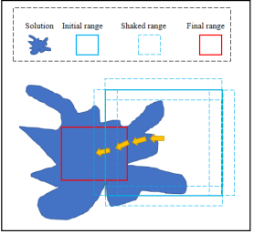
Figure 1: The heuristic search

The heuristic method can produce and compare results by itself, the calculation goes on until the best parameter ranges generate almost identical experimental results. Here is the method. First, input a set of parameter ranges, physical quantities calculated with these parameters are compared to experimental values. The probability that these calculated results match the experimental data can be obtained, it is proportional to the solution density. When the probability is less than 99.99$\%$, the parameters will change 30 percent automatically, and the probability will be recalculated. Repeat the calculation like this until the results are almost identical to the experimental values with a consistency of 99.99$\%$. The newly obtained parameter ranges are taken as the true ones. Fig.2 is the flowchart,

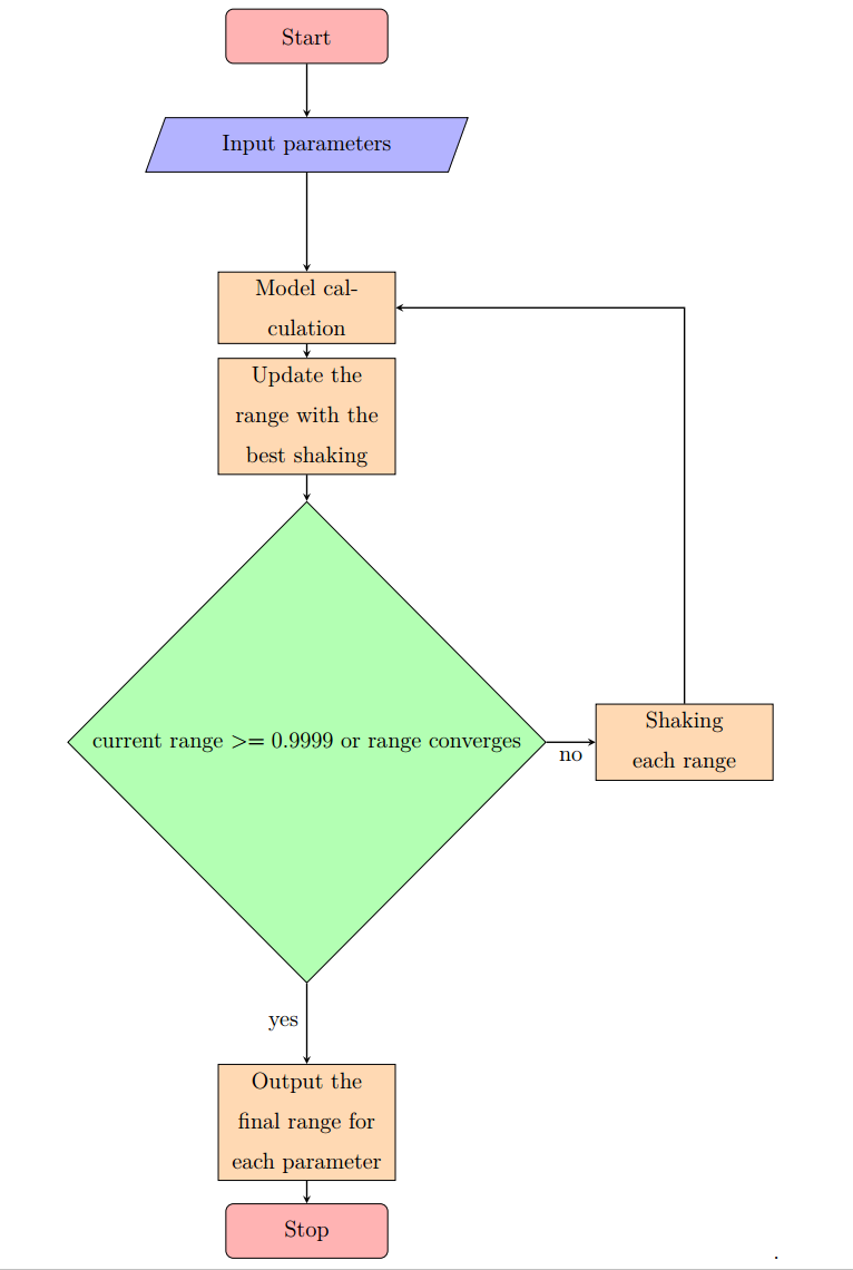
Figure 2: The Majorana phases

Even if the probability of the solution in the final ranges is as high as $0.9999$, it does not always mean the expected value is high. For instance, when we flip a fair coin, if X denotes the value of the coin flip with the head, then the expected value of the random quantity X is $1/2$. However, if we flip the coin ten times, it is possible to get the head every time. Ten times is not an ideal number of experiments. As long as we do enough many times coin-flipping experiments, the probability will close to the expected value. Similar to that situation, it is necessary to prove that picking 10,000 points randomly is reasonable. According to the Chernoff bound Buot2006Probability ,

$$\ P_{r}(X\geq(1+\delta)Np)\leq\frac{e^{\delta Np}}{(1+\delta)^{(1+\delta)Np}},\\$$ (6)

namely,

$$\ P_{r}(p\leq\frac{X}{(1+\delta)N})\leq\frac{e^{\delta Np}}{(1+\delta)^{(1+\delta)Np}},$$ (7)

where function $P_{r}(x)$ means the probability of $x$, $N$ is the total times, $X$ is the number of the valid points, and $\displaystyle\frac{X}{(1+\delta)N}$ approximately equals to the calculated probability with $\delta$ standing for the uncertainty of the probability. Let $p_{0}=\displaystyle\frac{X}{(1+\delta)N}$, $P_{r}(p\leq p_{0})$ is the probability that the expected value $p$ is smaller than $p_{0}$. Fig. 3 shows the relationship between $P_{r}(p\leq p_{0})$ and the probability $p_{0}$ when $N=10000$. As can be seen from this figure that the probability that the expected value $p$ is smaller than 0.98 is 0 when $N=10,000$ is chosen. In other words, the expected value is almost the same as the calculated probability.

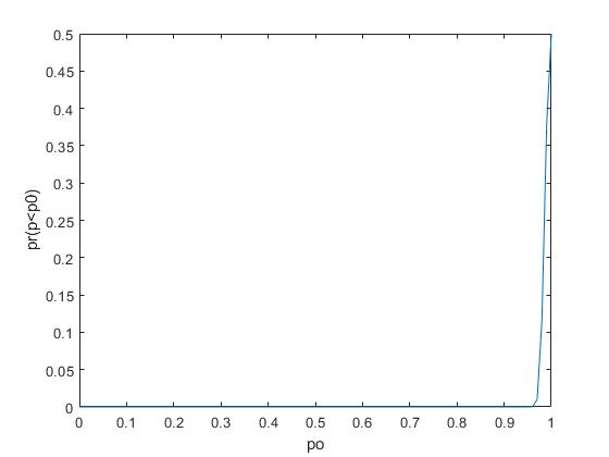
Figure 3: Relation of probability $P_{r}(p\leq p_{0})$ and expectation $p_{0}$ when $N=10000$. The abscissa $p_{0}$ indicates the calculated probability.

III.3 Experiments and results

The parameters in the model can be divided into two parts according to matrices (1) and (2), their ranges can be analyzed by the heuristic method. First, we consider the charged lepton sector. For initial ranges, we input all the dimensionless couplings $\lambda_{\tau}$, $\lambda_{\mu}$, $y_{\tau}$ to be in (0.01-1), $v_{l_{\alpha}}$ in (1-10) GeV and $\delta_{l_{e}}$, $\delta_{l_{\mu}}$ and $\delta_{d}$ in $(0-2\pi)$. Compared with experimental data Tanabashi:2018oca , $m_{\mu}=0.105$ GeV and $m_{\tau}=1.776$ GeV, the heuristic method can filter out the values of parameters by shaking, then the final ranges can be obtained.

In the neutrino sector, the final ranges from the charged lepton sector are taken as initial ranges. Moreover, other parameters $\lambda^{\prime}_{1}$, $\lambda^{\prime}_{2}$, $v_{l_{\tau}}$, $\delta_{Z,\lambda_{1}}$ and $\delta_{l_{\tau}}$ are also considered. For the normal neutrino mass ordering, after multiple feedback from comparing with experimental data by shaking, it is found that $\lambda^{\prime}_{1}\simeq 10$ GeV², and $\lambda^{\prime}_{2}\simeq 30$ GeV² as suitable initial values. As with the parameters in the charged lepton sector, we enter $v_{l_{\tau}}$ in (1-10) GeV, $\delta_{l_{\tau}}$ and $\delta_{\lambda_{1}}$ in $(0-2\pi)$ as the initial ranges. By repeating the shaking step, full parameter ranges are obtained. Note in this sector, we filter parameter value ranges with experimentally known neutrino mass squared differences ${\Delta m_{21}}^{2}=(7.53\pm 0.18)\times 10^{-5}$ eV² and ${\Delta m_{32}}^{2}=(2.51\pm 0.05)\times 10^{-3}$ eV² and the mixing angles $\sin^{2}{(\theta_{12})}=0.307\pm 0.013$, $\sin^{2}{(\theta_{23})}=0.417\pm 0.025$ and $\sin^{2}{(\theta_{13})}=(2.12\pm 0.08)\times 10^{-2}$ Tanabashi:2018oca .

On the other hand, for the case of the inverted neutrino mass ordering, by choosing $\lambda^{\prime}_{2}>\lambda^{\prime}_{1}$, it is found that the initial ranges should be $\lambda^{\prime}_{1}\simeq(5-10)$ GeV² and $\lambda^{\prime}_{2}\simeq(10-20)$ GeV². But it always gives out empty final ranges. This indicates that there is no natural solution for the inverted neutrino mass ordering.

IV Analysis and prediction

Because in the shaking step, range boundaries change randomly, there are different or disconnected solutions. Here we list three representative solutions in Tables 1, 2 and 3. As can be seen from Table 1, several dimensionless coefficients are almost fixed, whereas the phase $\delta_{d}$ can be chosen values almost from 0 to 2$\pi$. This means the later parameters are insensitive to the measured quantities. It is seen from Tables 2 and 3 that $\lambda^{\prime}_{1}$ and $\lambda^{\prime}_{2}$ make major contribution to the neutrino masses. They are also almost fixed.

Parameter	Initial range	Output range 1	Output range 2	Output range 3
$\delta_{{l_{e}}}$	0-$2\pi$	1.2566-1.5009	3.9609-4.6449	4.5752-5.1800
$\delta_{{l_{\mu}}}$	0-$2\pi$	5.2517-5.5449	5.2517-5.5449	2.7266-2.9156
$\delta_{d}$	0-$2\pi$	0.7540-1.4326	1.2566-3.1416	3.1416-6.2754
$y_{\tau}$	0.01- 1	0.4525 -0.4540	0.4525-0.4550	0.4540-0.4570
$\lambda_{\tau}$	0.01- 1	0.4886-0.4900	0.4876-0.4890	0.4886-0.4900
$\lambda_{\mu}$	0.01- 1	0.0600 -0.0602	0.0598-0.0604	0.0600-0.0606
$\delta_{l_{\tau}}$	0-$2\pi$	2.4288-2.500	2.4453-2.4712	2.4280-2.500
$\delta_{\lambda_{1}}$	0-$2\pi$	1.5800-1.800	1.6997-1.7396	2.7463-2.9515
$\delta_{Z}$	0-$2\pi$	0.0305-0.032	0.0312-0.0323	0.0318-0.0333

Table 1: The different out put of dimensionless parameter ranges

Parameter	Initial range (GeV)	Output range 1(GeV)	Output range 2(GeV)	Output range 3(GeV)
$v_{l_{e}}$	1-10	1.2532-1.2651	1.2585-1.2783	1.2617-1.2783
$v_{l_{\mu}}$	1-10	2.5767-2.5809	2.5712-2.5770	2.5712-2.5809
$v_{d}$	1-10	2.3572-2.3661	2.3511-2.3586	2.3607-2.3661
$v_{l_{\tau}}$	1-10	6.1352-6.200	6.0200-6.200	6.0788-6.0927

Table 2: The different output of dimensionful parameter ranges

Parameter	Initial range (GeV2)	Output range 1 (GeV2)	Output range 2 (GeV2)	Output range 3 (GeV2)
$\lambda^{\prime}_{1}$	10-11	11.5800-11.700	11.5320-11.6200	11.500-11.5720
$\lambda^{\prime}_{2}$	30-31	30.5000 -30.700	30.500-30.6200	30.500-30.700

Table 3: $\lambda^{\prime}_{1}$ and $\lambda^{\prime}_{2}$

With these determined parameter ranges, neutrino physical results can be calculated. Firstly, three neutrino masses are predicted as in Fig. 4. Three generation neutrino masses are $m_{\nu_{1}}\simeq 0.007$ eV, $m_{\nu_{2}}\simeq 0.011$ eV and $m_{\nu_{3}}\simeq 0.051-0.056$ eV.

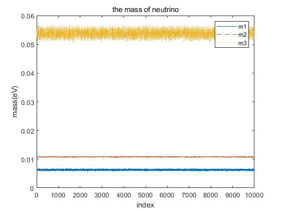
Figure 4: Neutrino masses

.

Secondly, the CP-violation phase $\delta_{CP}$ is generically large. The area of the unitarity triangle is calculated with obtained parameter ranges. Jarlskog invariant is twice of the area of the unitarity triangle, $\mathcal{J}=c_{12}c_{13}^{2}c_{23}s_{12}s_{13}s_{23}\sin\delta_{CP}\equiv\mathrm{Im}(V_{\alpha i}V_{\beta j}V_{\alpha j}^{*}V_{\beta i}^{*})$. $\mathcal{J}$ can be written as $\mathcal{J}=\mathcal{J}^{max}_{CP}\sin\delta_{CP}$ Esteban:2018azc . By choosing $\mathcal{J}^{max}_{CP}=0.033$, $\sin\delta_{CP}$ is calculated. Distribution of the CP violation phase is shown in Fig. 5. From the figure, $\sin\delta_{CP}\leq 0$, namely $\delta_{CP}$ takes values from $\pi$ to $2\pi$, and most probably $\sin\delta_{CP}\simeq-0.4$.

Thirdly, the effective Majorana mass in neutrinoless double $\beta$ decays is defined as $|\left\langle m_{ee}\right\rangle|=|m_{\nu_{1}}U^{2}_{e1}+m_{\nu_{2}}U^{2}_{e2}+m_{\nu_{3}}U^{2}_{e3}|$. The effective mass is shown in Fig. 6. Since 10,000 points are taken per range, we use ”index” in the abscissa in the figure to indicate the order of the valid points. The ordinate indicates the value of the effective mass calculated at each point. From the figure, it can be seen that the effective Majorana mass ranges from $5.5\times 10^{-3}$ eV to $8.5\times 10^{-3}$ eV. The order of magnitude of the effective Majorana neutrino mass is about $\sim 7\times 10^{-3}$ eV.

With the PMNS matrix given in the following form,

$$\begin{pmatrix}U_{e1}&U_{e2}&U_{e3}\\ U_{\mu 1}&U_{\mu 2}&U_{\mu 3}\\ U_{\tau 1}&U_{\tau 2}&U_{\tau 3}\\ \end{pmatrix}\begin{pmatrix}1&0&0\\ 0&e^{i\rho}&0\\ 0&0&e^{i\sigma}\\ \end{pmatrix},$$ (8)

the Majorana phases are given in Fig. 7. They are predicted as $\rho\simeq(0.44\pi-0.63\pi)$ and $\sigma\simeq(0.73\pi-1.01\pi)$.

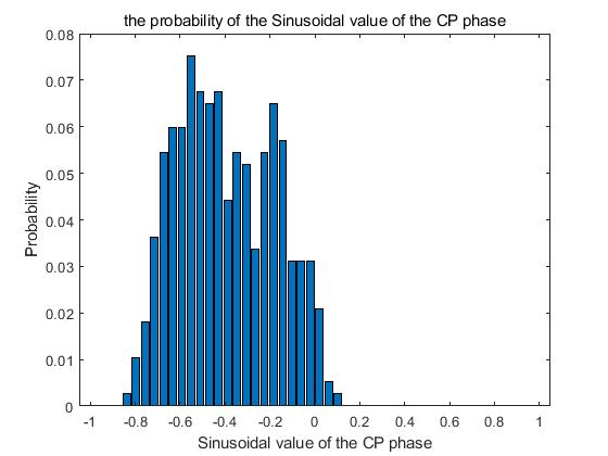
Figure 5: The distribution of the Dirac CP violation phase.

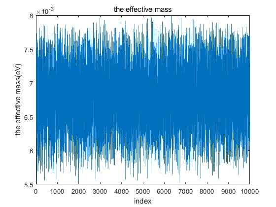
Figure 6: The range of effective Majorana neutrino mass.

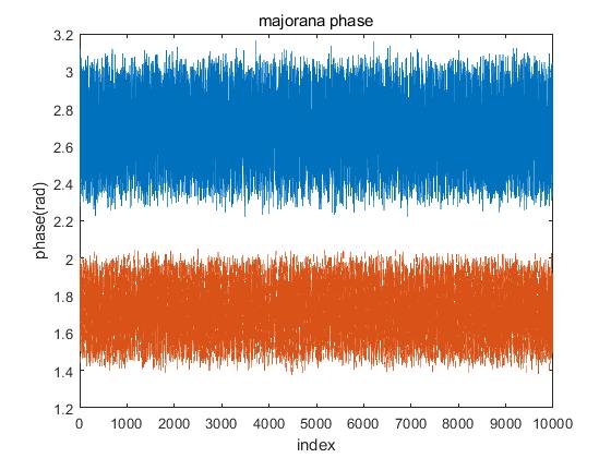
Figure 7: The Majorana phases.

It is necessary to check our last approximated anlysis of Ref. Lei:2018lln by this method. We take approximation in the previous work, that is, $\delta_{l\alpha}=0$ as the input condition. Repeating the process of the heuristic search, neutrino masses and the distribution of CP violation are obtained in Figs. 8 and 9, respectively. It is seen from the Fig. 8 that the masses of the first two generation neutrinos are almost the same, $m_{\nu_{1}}$ and $m_{\nu_{2}}$ are around 0.02 eV. These results are consistent with our previous predictions. Note, however, that the number of abscissa indices tells us that this solution is unlikely.

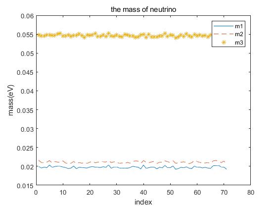
Figure 8: Neutrino masses of Lei:2018lln

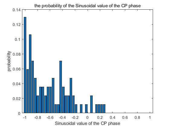
Figure 9: Distribution of the CP violation phase of Ref. Lei:2018lln

V Summary

We have tried to find out phenomenological consequences for neutrino physics of the high scale SUSY model for fermion masses. For the lepton mass matrices (1) and (2) obtained from the theory model, the heuristic method has been applied to find the most suitable solution for all the physical parameters numerically. And the Monte Carlo simulation has been also used to judge the reasonability of the results.

Probabilities that can match experimental data for different ranges of all the parameters have been calculated out. By constantly adjusting the range of parameters, we have finally found the maximum probability of solutions, to determine the most appropriate parameter values. Then the physical quantities can be calculated. Following results have been obtained. (1) The model only supports normal hierarchical neutrino mass pattern. The masses are that $m_{\nu_{1}}\simeq 0.007$ eV, $m_{\nu_{2}}\simeq 0.011$ eV, and $m_{\nu_{3}}\simeq 0.05$ eV. (2) The effective Majorana neutrino mass to be discovered in neutrinoless double $\beta$ decay experiments, is $7\times 10^{-3}$ eV. (3) The Dirac CP violating phase can be anywhere from $\pi$ to $2\pi$.

Finally, several discussions and remarks should be made. (1) Although the number of parameters is a kind of many, all the basic dimensionless coupling constants of the model are required to be in the natural range ($0.01-1$). What we have pursued here is to find phenomenological consequences of neutrino physics due to mass matrices (1) and (2) resulted from a high scale supersymmetry model. The results are physically meaningful. For example, inverted neutrino mass ordering is not allowed with our naturalness requirement. It is not trivial that right neutrino masses and mixings can be obtained without introducing in small parameters or accidentally large cancellation of the parameters. (2) It is necessary to compare our results in this work with that we obtained previously with approximation Lei:2018lln . Note that what we have obtained here is the most probable solution. Other solutions, like the one obtained in Ref. Lei:2018lln , is not ruled out. To be in detail, it is seen that the degeneracy of the first two generation neutrinos is not obvious compared to our previous work. $m_{\nu_{1,2}}$ are smaller than that in Ref. Lei:2018lln . This difference is due to the uncertainties of the parameters.

The effect of the phases of the sneutrino VEVs on the model is larger than we thought, especially that of $\delta_{l_{\tau}}$ and $\delta_{\lambda_{1}}$. Nevertheless, it is remarkable to note that, for each physical quantity, the result of this analysis and that in Ref. Lei:2018lln is in the same order. In terms of orders of magnitude, our results agree with previous ones. Thus we emphasize on that this model generically has the following neutrino mass pattern, $m_{\nu_{1,2}}\sim 10^{-2}$ eV and $m_{\nu_{3}}\sim 5\times 10^{-2}$ eV. This model once predicted large $\theta_{13}$ Liu:2005qic ; Liu:2012qua . But one number is not enough for justfying a model. The results obtained in this work will be further checked in the near future. One specific feature of the results is that the first two generation neutrino masses are very close to each other. This implies a relatively large effective Majorana neutrino mass to be measured in neutrinoless double beta decay experiments, meanwhile with normal mass ordering. (3) Our heuristic searching method is quite efficient. Compared to other methods, it has advantages in analyzing a given complex model with quite a lot of trigonometric function calculations, and in finding the range of dense solutions. It may have wider use in other complicated problems in particle physics.

- (1) K. Abe et al. Physics potential of a long-baseline neutrino oscillation experiment using a J-PARC neutrino beam and Hyper-Kamiokande. PTEP, 2015:053C02, 2015.
- (2) Babak Abi, R Acciarri, MA Acero, M Adamowski, C Adams, D Adams, P Adamson, M Adinolfi, Z Ahmad, CH Albright, et al. The dune far detector interim design report volume 1: Physics, technology and strategies. arXiv preprint arXiv:1807.10334, 2018.
- (3) R Acciarri, MA Acero, M Adamowski, C Adams, P Adamson, S Adhikari, Z Ahmad, CH Albright, T Alion, E Amador, et al. Long-baseline neutrino facility (LBNF) and deep underground neutrino experiment (DUNE) conceptual design report, volume 4 the dune detectors at lbnf. arXiv preprint arXiv:1601.02984, 2016.
- (4) Max Buot. Probability and computing: Randomized algorithms and probabilistic analysis. Publications of the American Statistical Association, 101(473):395–396, 2006.
- (5) Sascha Caron, Jong Soo Kim, and Krzysztof Rolbiecki . The bsm-ai project: Susy-ai-generalizing lhc limits on supersymmetry with machine learning. European Physical Journal C, 77(4), 2016.
- (6) Xun Chen et al. PandaX-III: Searching for neutrinoless double beta decay with high pressure136Xe gas time projection chambers. Sci. China Phys. Mech. Astron., 60(6):061011, 2017.
- (7) Zelimir Djurcic et al. JUNO Conceptual Design Report. arXiv preprint arXiv:1508.07166, 2015.
- (8) Ivan Esteban, M. C. Gonzalez-Garcia, Alvaro Hernandez-Cabezudo, Michele Maltoni, and Thomas Schwetz. Global analysis of three-flavour neutrino oscillations: synergies and tensions in the determination of , , and the mass ordering. JHEP, 01:106, 2019.
- (9) Wu-zhong Guo and Miao Li. A Possible Hermitian Neutrino Mixing Ansatz. Phys. Lett., B718:1385–1389, 2013.
- (10) Bo Hu. Neutrino Mixing and Discrete Symmetries. Phys. Rev., D87(3):033002, 2013.
- (11) Yoshiharu Kawamura. Study on fermion mass hierarchy due to vector-like fermions from the bottom up. 2019.
- (12) Ying-Ke Lei and Chun Liu. Neutrino phenomenology of a high scale supersymmetry model. Commun. Theor. Phys., 71(3):287, 2019.
- (13) Chun Liu. A supersymmetry model of leptons. Phys. Lett., B609:111–116, 2005.
- (14) Chun Liu. Supersymmetry for fermion masses. Commun. Theor. Phys., 47:1088–1098, 2007.
- (15) Chun Liu and Zhen-hua Zhao. and the Higgs mass from high scale supersymmetry. Commun. Theor. Phys., 59:467–471, 2013.
- (16) Jie Ren, Lei Wu, Jin Min Yang, and Jun Zhao. Exploring supersymmetry with machine learning. Nucl. Phys. B, 943:114613, 2019.
- (17) M. Tanabashi et al. Review of Particle Physics. Phys. Rev., D98(3):030001, 2018.
- (18) Zhen-hua Zhao. Understanding for flavor physics in the lepton sector. Phys. Rev., D86:096010, 2012.