Bilocal quantum criticality

Abstract

We consider 2+1 dimensional conformal gauge theories coupled to additional degrees of freedom which induce a spatially local but long-range in time $1/(\tau-\tau^{\prime})^{2}$ interaction between gauge-neutral local operators. Such theories have been argued to describe the hole-doped cuprates near optimal doping. We focus on a SU(2) gauge theory with $N_{h}$ flavors of adjoint Higgs fields undergoing a quantum transition between Higgs and confining phases: the $1/(\tau-\tau^{\prime})^{2}$ interaction arises from a spectator large Fermi surface of electrons. The large $N_{h}$ expansion leads to an effective action containing fields which are bilocal in time but local in space. We find a strongly-coupled fixed point at order $1/N_{h}$, with dynamic critical exponent $z>1$. We show that the entropy preserves hyperscaling, but nevertheless leads to a linear in temperature specific heat with a co-efficient which has a finite enhancement near the quantum critical point.

I Introduction

Strongly-coupled gauge theories in 2+1 spacetime dimensions play a fundamental role in many phenomena in quantum condensed matter physics. Of special interest are ‘deconfined’ critical points of such theories, which separate phases with different patterns of confinement, broken symmetry, and/or topological order. The best understood class of such critical points have an emergent relativistic conformal symmetry, allowing use of many tools from the conformal field theory literature. However, such conformal gauge theories apply to limited classes of phenomena in insulators or quantum Hall systems, and usually not to metallic, compressible systems with Fermi surfaces in the clean limit. In particular, conformal critical systems have a low temperature ($T$) specific heat $C_{v}\sim T^{2}$, which is smaller than the specific heat $C_{v}\sim T$ in metals.

Our interest in studying gauge theories of critical points in metals was motivated by numerous experimental indications Proust and Taillefer (2019); Vishik et al. (2012); He et al. (2014); Fujita et al. (2014); Badoux et al. (2016); Loram et al. (2001); Michon et al. (2019); Tallon et al. (2019); Tang et al. (2018); Chen et al. (2019); Panagopoulos et al. (2002, 2004); Frachet et al. (2019) of optimal doping criticality in the hole-doped cuprate superconductors. We examine here further aspects of a recently proposed Sachdev et al. (2019); Scammell et al. (2020) SU(2) gauge theory for the vicinity of optimal doping in which a parent conformal theory is coupled to a large Fermi surface of gauge-neutral electrons. This theory describes a phase transition from a Higgs phase, representing the pseudogap regime, to a confining phase, representing the overdoped Fermi liquid. The main effect of the spectator Fermi surface is a spatially local, but long-range in time interaction $\sim 1/(\tau-\tau^{\prime})^{2}$ between gauge-neutral local operators, where $\tau,\tau^{\prime}$ are the imaginary time co-ordinates of two such operators Sachdev and Morinari (2002); Nussinov and Zaanen (2002); Zaanen and Nussinov (2003); Grover and Senthil (2010); Kaul et al. (2008); Mross and Senthil (2012a, b). Within the context of a $1/N_{h}$ expansion, where $N_{h}$ is the number of flavors of Higgs fields, we find that this long-range interaction leads to a field theory that is bilocal in time, but local in space i.e. some fields depend upon one spatial co-ordinate $x$, and two time co-ordinates $\tau$ and $\tau^{\prime}$.

The bilocality is a consequence of the spectator Fermi surface. In the vicinity of conventional symmetry breaking transitions, Hertz Hertz (1976) argued that the low energy excitations on the Fermi surface could be accounted for by long-range interactions between the order parameter fields. Such arguments were extended to the SU(2) gauge theory in Ref. Sachdev et al., 2019, and in the case of interest to us, the long-range interactions induced by the large Fermi surface were irrelevant near the upper critical spatial dimension $d=3$. However, as we will describe in detail here, the long-range interactions are relevant for the SU(2) gauge theory in $d=2$ in the large $N_{h}$ limit, and lead to a bilocal field theory for computing the $1/N_{h}$ expansion.

We will find that the bilocal criticality is described by a new fixed point. This new fixed point is not relativistically invariant, and has dynamic critical exponent $z>1$ (see (75)). We show that the free energy preserves hyperscaling i.e its leading singular term is consistent with scaling dimension $d+z$. At first sight, this suggests that there is no contribution to a linear in $T$ specific heat from the singular hyperscaling preserving term. This turns out to not be the case. The specific heat is given by

$$C_{v}=\gamma_{b}\,T+T^{d/z}\,\Phi\left(\frac{T}{\Delta}\right)\,.$$ (1)

Here $\gamma_{b}T$ is the background and non-critical specific heat from the spectator Fermi surface; the prefactor $\gamma_{b}$ evolves smoothly across the critical point. The second term is the interesting, singular hyperscaling preserving term, with $\Phi$ a scaling function, and $\Delta$ an energy scale measuring the distance from the quantum critical point on the confining/Fermi liquid side. In the Fermi liquid regime, $T\ll\Delta$, this hyperscaling preserving term contributes $C_{v}/T\sim-\Delta^{d/z-1}$, and so yields a finite enhancement of $\lim_{T\rightarrow 0}C_{v}/T$ near the quantum critical point.

We note that bilocal field theories have appeared earlier in the context of systems with random interactions. Ref. Read et al., 1995 obtained a bilocal field theory for the Ising spin glass in a transverse field. Bilocal field theories also play a central role in models with random and all-to-all interactions, and in particular those related to the Sachdev-Ye-Kitaev (SYK) models Georges et al. (2000, 2001); Maldacena and Stanford (2016); Kitaev and Suh (2018); Gu et al. (2020). Our model appears to be the first realization in a non-random system, and the bilocality arises from a subtle interplay between the gauge-charged matter fields, and the Fermi surface of electrons. Given the phenomenological appeal of SYK models, the appearance of bilocality in more realistic models of cuprate physics is encouraging.

We will introduce our model field theory with bilocality in Section II. We describe $N_{h}=\infty$ saddle-point theory in Section III. A key ingredient in our analysis is the bilocal field $C(x,\tau,\tau^{\prime})$, and we describe its low $T$ saddle point value $C(\tau-\tau^{\prime})$ in Sections III.1-III.3. We will compute the free energy at $N_{h}=\infty$ in Section III.4. Full numerical solutions of the saddle point equations appears in Section III.5. We turn to a renormalization group analysis in Section IV, where we will obtain some results to order $1/N_{h}$, including the value of $z$ in (75).

II The Model

The gauge-charged matter sector of the model of Refs. Sachdev et al., 2019; Scammell et al., 2020 has real Higgs fields $H_{a\ell}$, where $a=1,2,3$ is the SU(2) adjoint gauge index, and $\ell=1\ldots N_{h}$ is the flavor index. This is coupled to SU(2) gauge field $A_{a\mu}$, where $\mu$ is a spacetime index. The Higgs field arises from a transformation of the spin density wave order parameter to a rotating reference frame, and optimal doping criticality is mapped onto the Higgs-confinement transition of such a gauge theory. The continuum action for the theory is $\int d^{d}xd\tau\mathcal{L}_{H}+\mathcal{S}_{f}$ (we set $d=2$) with the Lagrangian density

$$\mathcal{L}_{H}=\frac{1}{4g_{a}^{2}}F_{a\mu\nu}F_{a\mu\nu}+\frac{1}{2}\left(\partial_{\mu}H_{a\ell}-\varepsilon_{abc}A_{b\mu}H_{c\ell}\right)^{2}+V(H)$$ (2)

with the field strength

$$F_{a\mu\nu}=\partial_{\mu}A_{a\nu}-\partial_{\nu}A_{a\mu}-\varepsilon_{abc}A_{b\mu}A_{c\nu}\,,$$ (3)

and the Higgs potential

$$V(H) =\frac{{u}_{0}}{2N_{h}}\left[H_{a\ell}H_{a\ell}-\frac{3N_{h}}{g}\right]^{2}+\frac{{u}_{1}}{2N_{h}}H_{a\ell}H_{am}H_{b\ell}H_{bm}$$ (4)

The coupling $g$ is the tuning parameter across the Higgs transition. For $g<g_{c}$, we have the Higgs phase: this is proposed to describe the underdoped pseudogap regime of the cuprates, and its properties were discussed in detail in Ref. Sachdev et al., 2019. For $g>g_{c}$, the theory confines, and after including the spectator Fermi surface, we eventually obtain a conventional Fermi liquid description of the overdoped cuprates. Our focus in the body of the paper will be for values $g\geq g_{c}$ where there is no Higgs condensate

We can take the limit of strong quartic interactions $u_{0}\rightarrow\infty$ without modifying universal properties, and this simplifies the analysis and allows comparison with previous large $N_{h}$ work without gauge fields Chubukov et al. (1994); Podolsky and Sachdev (2012). The coupling $u_{1}$ is important in distinguishing possible Higgs phases for $g<g_{c}$, but it will not play a significant role for $g\geq g_{c}$. The gauge coupling $g_{a}$ will play no direct role in the large $N_{h}$ computations in this paper.

The effective potential $V(H)$ is constrained by the SU(2) gauge symmetry, and a global O($N_{h}$) symmetry acting on the flavor indices $\ell,m$. In the models considered in Ref. Sachdev et al., 2019, the global symmetry is smaller, and arises from the action of the square lattice space group symmetry on the charge density wave (and other) order parameters. We have enhanced the space group symmetry to O($N_{h}$) for simplicity Sachdev et al. (2019); Scammell et al. (2020).

The second term in the action is the long-range interaction obtained by integrating out the large Fermi surface of electrons.

$$\mathcal{S}_{f}=-\frac{1}{2N_{h}}\int d^{d}xd\tau d\tau^{\prime}H_{a\ell}(x,\tau)H_{am}(x,\tau)J_{f}(\tau-\tau^{\prime})H_{b\ell}(x,\tau^{\prime})H_{bm}(x,\tau^{\prime})$$ (5)

The electrons couple to the gauge-invariant order parameters

$$Q_{\ell m}=H_{a\ell}H_{am}-\frac{\delta_{\ell m}}{N_{h}}H_{an}H_{an},$$ (6)

and then integrating out the electrons leads to the index and spacetime structure in $\mathcal{S}_{f}$; this structure will be crucial to the appearance of bilocality. We are assuming here that $Q_{\ell m}$ correspond to order parameters at non-zero wavevectors, and in that case we expect Hertz (1976) $J_{f}(\tau)\sim 1/\tau^{2}$ at large $\tau$, which is the Fourier transform of a $|\omega|$ frequency dependence. In the more complete model of Ref. Sachdev et al., 2019, some of the $Q_{\ell m}$ correspond to order parameters at zero momentum, in which case the corresponding $J_{f}$ will be different: it will have both space and time dependencies arising from the Fourier transform of $|\omega|/|{\bm{k}}|$. We will not consider this more complex case here.

Our computations with $\mathcal{S}_{f}$ require an ultra-violet (UV) cutoff, and we choose

$$J_{f}(\tau)=\frac{K}{\varkappa^{2}+\tau^{2}}$$ (7)

where $\varkappa$ is a short time cutoff. This has a simple Fourier transform

$$\tilde{J}_{f}(\omega)=\frac{\pi K}{\varkappa}e^{-\varkappa|\omega|}$$ (8)

We will use the form in (8) but with Matsubara frequencies

$$\tilde{J}_{f}(\omega_{n})=\frac{\pi K}{\varkappa}e^{-\varkappa|\omega_{n}|}\,.$$ (9)

So the $T>0$ form of $J_{f}(\tau)$ is

$$J_{f}(\tau) = \frac{\pi KT\sinh(2\varkappa\pi T)}{\varkappa\left[\cosh(2\varkappa\pi T)-\cos(2\pi T\tau)\right]}.$$ (10)

To obtain the large $N_{f}$ limit, we decouple $\mathcal{S}_{f}$ by introducing a bilocal field $C_{ab}(x,\tau,\tau^{\prime})$, and the terms in $V(H)$ with local fields $B_{0}(x,\tau)$, $B_{1,ab}(x,\tau)$. In this manner, we obtain the partition function

$$\mathcal{Z} =\int\mathcal{D}C_{ab}(x,\tau,\tau^{\prime})\mathcal{D}B_{0}(x,\tau)\mathcal{D}B_{1,ab}(x,\tau)\mathcal{D}H_{a\ell}e^{-\mathcal{S}_{f}-\mathcal{S}_{b}}$$

$$\mathcal{S}_{f} =\int d^{d}xd\tau d\tau^{\prime}\left[\frac{N_{h}}{2}\frac{\left[C_{ab}(x,\tau,\tau^{\prime})\right]^{2}}{J_{f}(\tau-\tau^{\prime})}-C_{ab}(x,\tau,\tau^{\prime})H_{a\ell}(x,\tau)H_{b\ell}(x,\tau^{\prime})\right],$$

$$\mathcal{S}_{b} =\frac{1}{2}\int d^{d}xd\tau\Biggl{[}\left[\partial_{\mu}H_{a\ell}(x,\tau)\right]^{2}+iB_{0}(x,\tau)\left(H_{a\ell}(x,\tau)H_{a\ell}(x,\tau)-\frac{3N_{h}}{g}\right)+\frac{N_{h}\left[B_{0}(x,\tau)\right]^{2}}{4u_{0}}$$

$$~{}~{}~{}~{}~{}~{}~{}~{}~{}~{}~{}~{}~{}~{}~{}~{}~{}~{}~{}+iB_{1,ab}(x,\tau)H_{a\ell}(x,\tau)H_{b\ell}(x,\tau)+\frac{N_{h}\left[B_{1,ab}(x,\tau)\right]^{2}}{4u_{1}}\Biggr{]}.$$ (11)

In the large $N_{h}$ limit, we integrate over the $H_{a\ell}$ and obtain an effective action for the $C_{ab}$, $B_{0}$, and $B_{1,ab}$ with a prefactor of $N_{h}$. Note that the bilocal field $C_{ab}(x,\tau_{1},\tau^{\prime})$ is included in this effective action. The large $N_{h}$ limit then involves the saddle point analysis of this action, which we present in the following sections.

III Large $N_{h}$ limit

For the symmetric phase, at the large $N_{h}$ saddle point, we take the following gauge invariant ansatz

$$C_{ab}(x,\tau,\tau^{\prime}) =\delta_{ab}C(\tau-\tau^{\prime}),$$

$$iB_{0}(x,\tau) =B_{0},$$

$$iB_{1,ab}(x,\tau) =\delta_{ab}B_{1}.$$ (12)

From (11) we observe that

$$\frac{3B_{1}}{2u_{1}}=\frac{B_{0}}{2u_{0}}+\frac{1}{g}=\frac{1}{N_{h}}\left\langle H_{a\ell}^{2}\right\rangle$$ (13)

We can therefore express $B_{1}$ in terms of $B_{0}$ everywhere, and only treat $B_{0}$ as an independent variable. Let us also introduce $\tilde{C}(\omega_{n})$ as the Fourier transform of $C(\tau)$, and define the parameter

$$[\Delta(T)]^{2}\equiv B_{0}+B_{1}-2\tilde{C}(0)\,,$$ (14)

where we explicitly identify the $T$ dependence to distinguish it from $\Delta\equiv\Delta(T=0)$. We will see below that $[\Delta(T)]^{-1}$ is best understood as a spatial correlation length $\xi_{x}$, and not a temporal correlation length $\xi_{\tau}$; hence we do not call it a ‘gap’. Then, in the limit $u_{0}\rightarrow\infty$ the free energy density $F$ is a functional only of $\Delta(T)$ and $C(\tau)$ given by (after dropping an additive constant)

$$\frac{F[\Delta(T),C(\tau)]}{3N_{h}} = \frac{1}{2}\int_{0}^{\beta}d\tau\frac{\left[C(\tau)\right]^{2}}{J_{f}(\tau)}+\frac{T}{2}\sum_{\omega_{n}}\int^{\Lambda}\frac{d^{2}k}{4\pi^{2}}\ln\bigl{[}k^{2}+\omega_{n}^{2}+[\Delta(T)]^{2}-2\tilde{C}(\omega_{n})+2\tilde{C}(0)\bigr{]}$$ (15)

$$~{}~{}~{}~{}~{}~{}~{}~{}~{}~{}~{}~{}~{}~{}~{}~{}~{}~{}-\frac{[\Delta(T)]^{2}+2\tilde{C}(0)}{2g}\,.$$

Here $\beta=1/T$, and $\Lambda$ is large momentum cutoff which we impose by a Pauli-Villars subtraction (see Section III.5). Our task in this section is to solve the saddle-point equations of $F$, and then determine $F$ as a function of $T$ and $g$.

The saddle point equations of (15) are

$$C(\tau) = J_{f}(\tau)\int^{\Lambda}\frac{d^{2}k}{4\pi^{2}}G(k,\tau)$$ (16)

$$\frac{1}{g} = \int^{\Lambda}\frac{d^{2}k}{4\pi^{2}}G(k,0)$$ (17)

where the Higgs field Green’s function is

$$\tilde{G}(k,\omega_{n})=\frac{1}{k^{2}+\omega_{n}^{2}+[\Delta(T)]^{2}-2\tilde{C}(\omega_{n})+2\tilde{C}(0)}$$ (18)

and $G(k,\tau)$ is its Fourier transform in frequency/time. We have to solve (16) and (17) for $\Delta(T)$ and $C(\tau)$ as a function of $T$ and $g$. In practice, it is easier to pick a value of $\Delta(T)$, solve (16) for $C(\tau)$, and then determine the value of $g$ as a dependent variable from (17). In particular, the critical value $g_{c}$ is determined by following this procedure for $\Delta(T=0)=0$.

III.1 Critical point

First, let us examine the nature of the critical point at $g=g_{c}$ at $T=0$. Let us assume the power-law behavior

$$C(\tau)=\frac{\kappa_{0}}{|\tau|^{\alpha}}\quad\mbox{as $|\tau|\rightarrow\infty$},$$ (19)

for some exponent $\alpha$ and prefactor $\kappa_{0}$. Then

$$\tilde{C}(\omega)-\tilde{C}(0)=2\kappa_{0}|\omega|^{\alpha-1}\Gamma(1-\alpha)\sin(\pi\alpha/2)\quad\mbox{as $|\omega|\rightarrow 0$}.$$ (20)

We can drop the $\omega_{n}^{2}$ term in (18) if $\alpha<3$. So we evaluate

$$\int\frac{d^{d}kd\omega}{(2\pi)^{d+1}}\tilde{G}(k,\omega)e^{-i\omega\tau} \approx \int\frac{d^{d}kd\omega}{(2\pi)^{d+1}}\frac{e^{-i\omega\tau}}{k^{2}-4\kappa_{0}|\omega|^{\alpha-1}\Gamma(1-\alpha)\sin(\pi\alpha/2)}$$

$$= \frac{\Gamma(1-d/2)}{(4\pi)^{d/2}}\int\frac{d\omega}{2\pi}e^{-i\omega\tau}\left[-4\kappa_{0}|\omega|^{\alpha-1}\Gamma(1-\alpha)\sin(\pi\alpha/2)\right]^{(d-2)/2}$$

$$= -\frac{\Gamma(1-d/2)}{(4\pi)^{d/2}}\left[-4\kappa_{0}\Gamma(1-\alpha)\sin(\pi\alpha/2)\right]^{(d-2)/2}\left[\frac{\Gamma(1+\delta)\sin(\pi\delta/2)}{\pi|\tau|^{1+\delta}}\right]$$

where

$$\delta\equiv\frac{(\alpha-1)(d-2)}{2}$$ (22)

From saddle point equation (16), we now see that $\delta+3=\alpha$ or

$$\alpha=\frac{8-d}{4-d}=3-(2-d)+\ldots\quad\mbox{as $d\rightarrow 2$}\,,$$ (23)

and

$$\kappa_{0} = \left(-K\frac{\Gamma(1-d/2)}{(4\pi)^{d/2}}\left[-4\Gamma(1-\alpha)\sin(\pi\alpha/2)\right]^{(d-2)/2}\left[\frac{\Gamma(1+\delta)\sin(\pi\delta/2)}{\pi}\right]\right)^{2/(4-d)}$$ (24)

$$= \frac{K}{4\pi}\quad\mbox{as $d\rightarrow 2$}.$$

So we have a well-behaved result in the limit $d\rightarrow 2$ of interest to us:

$$C(\tau)=\frac{K}{4\pi|\tau|^{3}}\quad\mbox{for $d=2$}\,.$$ (25)

Note that this result is linear in $K$, although we did not make an expansion in $K$ above; our analysis was only a low frequency asymptotic analysis. It can now be verified that computing the term linear in $K$ from (16) by dropping the $\tilde{C}$ contribution to $G$ on the right-hand-side also yields (25).

For the frequency dependence, the above results imply

$$\tilde{C}(0)-\tilde{C}(\omega)=\frac{K\omega^{2}}{4\pi(2-d)}\quad\mbox{as $d\rightarrow 2$}.$$ (26)

By the usual interpretation of dimensional regularization, we conclude

$$\tilde{C}(0)-\tilde{C}(\omega)=\frac{K\omega^{2}\ln(\Lambda/|\omega|)}{4\pi}\quad\mbox{for $d=2$}.$$ (27)

III.1.1 Subleading terms

It is useful to examine the structure of the subleading corrections to (27) at low frequency, along with their dependence on $K$. Inserting (27) into the right-hand-side of (16), transforming to frequency space, and performing the momentum integral, we obtain

$$\tilde{C}(\omega)=\frac{K}{4}\int\frac{d\Omega}{2\pi}|\omega-\Omega|\ln\left[\frac{K\Omega^{2}\ln(\Lambda/|\Omega|)}{2\pi\Lambda^{2}}\right]$$ (28)

Taking a derivative, we have for $\omega>0$

$$\frac{d\tilde{C}(\omega)}{d\omega} = \frac{K}{4}\int\frac{d\Omega}{2\pi}\mbox{sgn}(\omega-\Omega)\ln\left[\frac{K\Omega^{2}\ln(\Lambda/|\Omega|)}{2\pi\Lambda^{2}}\right]$$ (29)

$$\approx \frac{K}{4\pi}\omega\ln\left[\frac{K\omega^{2}\ln(\Lambda/|\omega|)}{2\pi\Lambda^{2}}\right]$$

This agrees with (27), and yields a subleading correction which is suppressed by a factor of $\sim\ln[K\ln(\Lambda/|\omega|)]/\ln(\Lambda/|\omega|)$. We expect similar $\ln\ln/\ln$ corrections to all other aspects of the critical behavior to be discussed below.

III.2 Fermi liquid regime

Let us now increase $g$ above $g_{c}$ to gap the Higgs field in the Fermi liquid phase at $T=0$. We generalize the ansatz for $C(\tau)$ in (19) to

$$C(\tau)=\frac{\kappa_{1}e^{-|\tau|/\xi_{\tau}}}{|\tau|^{3}}\quad\mbox{as $|\tau|\rightarrow\infty$}.$$ (30)

Then by Fourier transform,

$$\tilde{C}(0)-\tilde{C}(\omega) = \frac{\kappa_{1}}{\sqrt{2\pi}}\ln\left(\xi_{\tau}e^{-\gamma}\right)\omega^{2}+O(\omega^{4})\ \ \ \ \mbox{as $|\omega|\rightarrow 0$}.$$ (31)

We now confirm via the saddle point equations that the ansatz (30) is self-consistent. For convenience, define $\tilde{\kappa}_{1}\equiv\kappa_{1}\ln\left(\xi_{\tau}e^{-\gamma}\right)/\sqrt{2\pi}$. We approximate the Greens function in the small $\omega$ limit, and again evaluate using dimensional regularization (we define $\Delta\equiv\Delta(T=0)$),

$$\int\frac{d^{d}kd\omega}{(2\pi)^{d+1}}G(k,\omega)e^{-i\omega\tau} \approx \int\frac{d^{d}kd\omega}{(2\pi)^{d+1}}\frac{e^{-i\omega\tau}}{k^{2}+\omega^{2}+\Delta^{2}+2\tilde{\kappa}_{1}\omega^{2}}$$ (32)

$$= \frac{\Gamma(1-d/2)}{(4\pi)^{d/2}}\int\frac{d\omega}{2\pi}e^{-i\omega\tau}\left[\omega^{2}(1+2\tilde{\kappa}_{1})+\Delta^{2}\right]^{(d-2)/2}$$

$$= \left[\frac{2\left(2\Delta^{2}\right)^{(d/2-1)}\left(\frac{1+2\tilde{\kappa}_{1}}{\Delta^{2}}\right)^{\frac{1}{4}(2(d/2-1)-1)}K_{(d/2-1)+\frac{1}{2}}\left(\left|\tau\right|\sqrt{\frac{\Delta^{2}}{1+2\tilde{\kappa}_{1}}}\right)}{(4\pi)^{d/2}\left|\tau\right|^{(d/2-1)+\frac{1}{2}}}\right]$$

$$= \frac{1}{2\sqrt{2\pi}}\frac{\sqrt{2\pi}e^{-\left|\tau\right|\sqrt{\frac{\Delta^{2}}{1+2\tilde{\kappa}_{1}}}}}{\left|\tau\right|}\ \ \ \ \mbox{at $d=2$}.$$

Here, $K_{n}$ is a Bessel function. Hence, asymptotically ($\tau\to\infty$) we have that

$$C(\tau) = J_{f}(\tau)G(\bm{x}=\bm{0},\tau)=\frac{K}{2\sqrt{2\pi}}\frac{e^{-\left|\tau\right|\sqrt{\frac{\Delta^{2}}{1+2\tilde{\kappa}_{1}}}}}{\left|\tau\right|^{3}},$$ (33)

which is consistent with (30) once we identify $\kappa_{1}=K/\sqrt{8\pi}$ and

$$\xi_{\tau} = \sqrt{1+K\ln\left(\xi_{\tau}e^{-\gamma}\right)/(2\pi)}\Delta^{-1}$$ (34)

$$\approx \frac{1}{\Delta}\left[\frac{K}{2\pi}\ln(\Lambda/\Delta)\right]^{1/2}$$

to leading logs.

We now determine the dependence of $\Delta$ on $(g-g_{c})$. We obtain this by writing the difference of (17) at $g=g_{c}$ and $g>g_{c}$ as

$$\int\frac{d\omega}{2\pi}\int^{\Lambda}\frac{d^{2}k}{4\pi^{2}}\left[\frac{1}{k^{2}+\omega^{2}K\ln(\bullet)/(2\pi)}-\frac{1}{k^{2}+\Delta^{2}+\omega^{2}K\ln(\bullet)/(2\pi)}\right]=\frac{1}{g_{c}}-\frac{1}{g}\,.$$ (35)

Here $\ln(\bullet)$ refers to a logarithm of various possible frequency scales. In the leading logarithm approximation discussed in Section III.1.1, we can just replace the logarithm by a constant with $\bullet=\Lambda/$(largest of external frequency scales); it can be verified that all of the results obtained so far in this section can also be obtained in this manner. Then (35) yields

$$\frac{\Delta}{4\pi}\left[\frac{K}{2\pi}\ln(\Lambda/\Delta)\right]^{-1/2}=\frac{1}{g_{c}}-\frac{1}{g}$$ (36)

or $\Delta\sim(g-g_{c})\ln^{1/2}(1/(g-g_{c}))$.

From (34) and (36), we see that $\xi_{\tau}^{-1}\sim(g-g_{c})$, without a logarithmic correction. The absence of logarithmic corrections in $\xi_{\tau}$ will be crucial to our results. Also, from the structure of the Green’s function, we see that the spatial correlation length, $\xi_{x}\sim\Delta^{-1}$. So there is a logarithmic singularity in the spatial correlation length, $\xi_{x}$, but not in the temporal correlation length $\xi_{\tau}$.

III.3 Non-zero temperatures

The solution at $T>0$ is characterized by the parameter $\Delta(T)$. We can determine $\Delta(T)$ in terms of $\Delta\equiv\Delta(T=0)$, the parameter at the same value $g$ at $T=0$; the method leading to (35) now yields

$$\int^{\Lambda}\frac{d^{2}k}{4\pi^{2}}\left[\int\frac{d\omega}{2\pi}\frac{1}{k^{2}+\Delta^{2}+\omega^{2}K\ln(\bullet)/(2\pi)}-T\sum_{\omega_{n}}\frac{1}{k^{2}+[\Delta(T)]^{2}+\omega_{n}^{2}K\ln(\bullet)/(2\pi)}\right]=0\,.$$ (37)

This yields an equation for $\Delta(T)$ which is the same as that in Ref. Chubukov et al., 1994 apart from the $\ln(\bullet)$ factors:

$$\frac{\Delta(T)}{T}\left[\frac{K}{2\pi}\ln(\bullet)\right]^{-1/2}=\Psi_{\Delta}\left(\frac{\Delta}{T}\left[\frac{K}{2\pi}\ln(\bullet)\right]^{-1/2}\right)\,,$$ (38)

where the scaling function $\Psi_{\Delta}$ is the same as Ref. Chubukov et al., 1994

$$\Psi_{\Delta}(y)=2\,\mbox{arcsinh}\left(\frac{e^{y/2}}{2}\right)\,.$$ (39)

In particular, at the critical point $g=g_{c}$, we have $\Delta=0$ and

$$\Delta(T)=\Theta T\left[\frac{K}{2\pi}\ln\left(\frac{\Lambda}{T}\right)\right]^{1/2}$$ (40)

where $\Theta=2\ln((\sqrt{5}+1)/2)$.

By combining (38) with (34), we see that there is no logarithmic prefactor in the time-correlation length, as we observed above

$$\xi_{\tau}^{-1}(T)=T\Psi_{\Delta}\left(\frac{\Delta}{T}\left[\frac{K}{2\pi}\ln(\bullet)\right]^{-1/2}\right)\,,$$ (41)

so that $\xi_{\tau}(T)=1/(\Theta T)$ at the critical point $g=g_{c}$, just as in Ref. Chubukov et al., 1994. For the function $C(\tau)$, the leading-log corrections can be absorbed into $\xi_{\tau}$, and we expect from (33) that

$$C(\tau)=\frac{1}{|\tau|^{3}}\Psi_{C}\left(\tau/\xi_{\tau}\right)\,,$$ (42)

with a scaling function $\Psi_{C}$.

III.4 Free energy

As we will describe below, evaluating the free energy in (15) leads to subtle questions on the nature of the low $T$ limit. It turns out to be essential to have full analytical control in order to separate terms with different physical origins. We already observed below (25) that perturbation theory in $K$ was sufficient in determining the asymptotic form of $C(\tau)$. And we will see in Section IV the critical coupling $K\sim 1/N_{h}$, which also justifies working at small $K$. We therefore divide the free energy as

$$F=F_{H}+F_{K}$$ (43)

where $F_{H}$ is the large-$N$ contribution of the Higgs field, and $F_{K}$ contains contributions from the large Fermi surface which are first order in $K$. The analysis below amounts to an expansion in the free energy to linear order in $K$ about the critical point $g=g_{c}$. However the value of $g_{c}$ itself depends upon $K$, and this effect has to be treated more carefully.

III.4.1 Evaluation of $F_{H}$

At zeroth order in $K$, the Higgs field contribution in (15) is the same as the free energy computed in Ref. Chubukov et al., 1994.

$$\frac{F_{H}(1/g,T)}{3N_{h}}=\frac{T}{2}\sum_{\omega_{n}}\int^{\Lambda}\frac{d^{2}k}{4\pi^{2}}\ln\bigl{[}k^{2}+\omega_{n}^{2}+[\Delta(T)]^{2}\bigr{]}-\frac{[\Delta(T)]^{2}}{2g}\,.$$ (44)

In this expression (and in the remainder of Section III.4), it is implied that $\Delta(T)$ is to be evaluated at the saddle point of (44) with respect to $\Delta(T)$. We write the saddle point equation (17), in a manner analogous to (37), as

$$\int^{\Lambda}\frac{d^{2}k}{4\pi^{2}}\left(T\sum_{\omega_{n}}\frac{1}{k^{2}+\omega_{n}^{2}+[\Delta(T)]^{2}}-\int\frac{d\omega}{2\pi}\frac{1}{k^{2}+\omega^{2}}\right)=\frac{1}{g}-\frac{1}{g_{c}^{0}}$$ (45)

where $g_{c}^{0}=4\pi/\Lambda$ is critical coupling at which $\Delta(T=0)=0$.

However, before inserting the evaluation of (44) into (43), we have to apply a renormalization procedure which is entirely analogous to converting perturbative field-theoretic expansions of critical phenomena from ‘bare’ mass propagators to ‘renormalized’ mass propagators, in which some perturbative terms are included to all orders Amit (1984). Here, this is essential for ensuring that our perturbative results in powers of $K$ hold not only in the perturbative regime where $K\Lambda\ll T$, but also in the limit $T\rightarrow 0$ at the critical point. In the present context, the ‘mass’ is the distance of coupling $1/g$ from the critical point $1/g_{c}$. At first order in $K$ there is a correction to the value of $1/g_{c}$ which is computed in Appendix A to be

$$\frac{1}{g_{c}}=\frac{1}{g_{c}^{0}}+\frac{1}{g_{c}^{1}}\quad;\quad\frac{1}{g_{c}^{1}}=-\frac{K\Lambda}{8\pi^{2}}\left(2\ln 2-\frac{1}{2}\right)\,,\quad\mbox{as $\varkappa\rightarrow 0$.}$$ (46)

So we introduce a ‘renormalized’ coupling $1/g_{R}$ related to the ‘bare’ coupling $1/g$ via

$$\frac{1}{g_{R}}-\frac{1}{g_{c}^{0}}=\frac{1}{g}-\frac{1}{g_{c}}\quad\Rightarrow\quad\frac{1}{g}=\frac{1}{g_{R}}+\frac{1}{g_{c}^{1}}\,.$$ (47)

Now when we evaluate the zeroth order expressions (44) and (45) at the renormalized coupling $1/g_{R}$ we obtain at $T=0$

$$\int^{\Lambda}\frac{d^{2}k}{4\pi^{2}}\int\frac{d\omega}{2\pi}\left[\frac{1}{k^{2}+\omega^{2}+\Delta^{2}}-\frac{1}{k^{2}+\omega^{2}}\right]=\frac{1}{g_{R}}-\frac{1}{g_{c}^{0}}\,.$$ (48)

Now we see from (47) that $\Delta=0$ precisely when the renormalized ‘mass’ $1/g_{R}-1/g_{c}^{0}$ vanishes at the true critical point where $g=g_{c}$. After the substitution in (47), we treat $1/g_{R}$ as independent of $K$, and expand everything in powers of the perturbative coupling $K$, just as is done in renormalized mass expansions in field theory. So we need to evaluate $F_{H}(1/g,T)=F_{H}(1/g_{R}+1/g_{c}^{1},T)$ to linear order in $K$. Here, we are aided by the fact that $F_{H}$ is a saddle point with respect to variations in $\Delta(T)$, so we need not account for the shift in $\Delta(T)$ to linear order. Indeed, we need only consider the variation arising from the only explicit linear dependence of (44) on $1/g$. So we have from (44) and (47)

$$F_{H}(1/g,T)=F_{H}(1/g_{R},T)-\frac{[\Delta(T)]^{2}}{2g_{c}^{1}}$$ (49)

Finally, we collect together the results of Section III.4.1, perform the frequency summations in (44) and (45) to obtain the final expression for $F_{H}$

$$\frac{F_{H}}{3N_{h}} = \frac{\Lambda^{3}}{12\pi}+\int^{\Lambda}\frac{d^{2}k}{4\pi^{2}}\Biggl{[}\frac{1}{2}\sqrt{k^{2}+[\Delta(T)]^{2}}-\frac{k}{2}+T\ln\left(1-e^{-\sqrt{k^{2}+[\Delta(T)]^{2}}/T}\right)$$ (50)

$$~{}-\frac{[\Delta(T)]^{2}}{4\sqrt{k^{2}+[\Delta(T)]^{2}}}\left\{1+2n\left(\sqrt{k^{2}+[\Delta(T)]^{2}}\right)\right\}\Biggr{]}-\frac{\left[\Delta(T)\right]^{2}}{2g_{c}^{1}}\,,$$

where $n(a)=1/(e^{a/T}-1)$ is the Bose function, and the value of $\Delta(T)$ is related to $\Delta$ by

$$\int^{\Lambda}\frac{d^{2}k}{4\pi^{2}}\left[\frac{1}{2\sqrt{k^{2}+[\Delta(T)]^{2}}}\left\{1+2n\left(\sqrt{k^{2}+[\Delta(T)]^{2}}\right)\right\}-\frac{1}{2\sqrt{k^{2}+\Delta^{2}}}\right]=0\,.$$ (51)

The integrals over $k$ are convergent as $\Lambda\rightarrow\infty$ in both (50) and (51). Consequently, the corresponding contribution to the free energy scales as $T^{3}\Phi_{H}(\Delta/T)$, where the scaling function $\Phi_{H}$ was given in Ref. Chubukov et al., 1994. The renormalized coupling $g_{R}$ appears only in determining the value of $\Delta$ in (48), and we will express all remaining results in this section in terms of $\Delta$. In $F_{K}$ we can simply replace $1/g$ by $1/g_{R}$, because those terms are already first order in $K$.

III.4.2 Evaluation of $F_{K}$

We turn next to the term $F_{K}$ in $F$, which contains all terms which are linear in $K$ corrections to $F_{H}$ in (44). We can obtain these terms simply by evaluating the expectation value of $\mathcal{S}_{f}$ in (5) in the large $N_{h}$ limit. So we obtain

$$\frac{F_{K}}{3N_{h}}=-\frac{1}{2}\int_{0}^{\beta}d\tau J_{f}(\tau)G^{2}(x=0,\tau)$$ (52)

or in frequency space

$$\frac{F_{K}}{3N_{h}}=-\frac{1}{2}T^{2}\sum_{\omega_{n},\epsilon_{n}}\tilde{J}_{f}(\omega_{n})\left[\int^{\Lambda}\frac{d^{2}k}{(2\pi)^{2}}\tilde{G}(k,\epsilon_{n})\right]\left[\int^{\Lambda}\frac{d^{2}p}{(2\pi)^{2}}\tilde{G}(p,\epsilon_{n}-\omega_{n})\right]$$ (53)

In (53) we use the Green’s function in (18) at zeroth order in $K$

$$\tilde{G}(k,\omega_{n})=\frac{1}{k^{2}+\omega_{n}^{2}+[\Delta(T)]^{2}}\,.$$ (54)

To compute the free energy, we first evaluate the summation over $\epsilon_{n}$ in (53) using the identity

$$T\sum_{\epsilon_{n}}\frac{1}{(\epsilon_{n}^{2}+a^{2})((\epsilon_{n}-\omega_{n})^{2}+b^{2})}=\frac{1}{2ab}\left[\frac{(b-a)(n(a)-n(b))}{\omega_{n}^{2}+(a-b)^{2}}+\frac{(a+b)(1+n(a)+n(b))}{\omega_{n}^{2}+(a+b)^{2}}\right]\,.$$ (55)

We also use (8) to evaluate by the contour integration method

$$T\sum_{\omega_{n}}\frac{\tilde{J}_{f}(\omega_{n})}{\omega_{n}^{2}+c^{2}}=\frac{\pi K\cos(\varkappa c)}{2\varkappa c}(1+2n(c))+\frac{K}{\varkappa}\int_{0}^{\infty}d\Omega\,\mathcal{P}\left(\frac{1}{c^{2}-\Omega^{2}}\right)\sin(\varkappa\Omega)(1+2n(\Omega))$$ (56)

Combining (53,55,56), and changing variables of integration from $k,p$ to $a=(k^{2}+[\Delta(T)]^{2})^{1/2}$, $b=(p^{2}+[\Delta(T)]^{2})^{1/2}$ we obtain

$$\frac{F_{K}}{3N_{h}} = -\frac{1}{16\pi^{2}}\int_{\Delta(T)}^{\sqrt{\Lambda^{2}+[\Delta(T)]^{2}}}da\int_{\Delta(T)}^{\sqrt{\Lambda^{2}+[\Delta(T)]^{2}}}db\Biggl{[}\frac{\pi K\cos(\varkappa(a-b))}{2\varkappa}(1+2n(a-b))(n(b)-n(a))$$

$$~{}~{}~{}~{}~{}~{}~{}+\frac{\pi K\cos(\varkappa(a+b))}{2\varkappa}(1+2n(a+b))(1+n(b)+n(a))$$

$$~{}~{}~{}~{}~{}~{}~{}+\frac{K}{\varkappa}\int_{0}^{\infty}d\Omega\,\mathcal{P}\left(\frac{1}{(a-b)^{2}-\Omega^{2}}\right)\sin(\varkappa\Omega)(1+2n(\Omega))(b-a)(n(a)-n(b))$$

$$~{}~{}~{}~{}~{}~{}~{}+\frac{K}{\varkappa}\int_{0}^{\infty}d\Omega\,\mathcal{P}\left(\frac{1}{(a+b)^{2}-\Omega^{2}}\right)\sin(\varkappa\Omega)(1+2n(\Omega))(a+b)(1+n(a)+n(b))\Biggr{]}\,.$$

Details of the evaluation of the integrals in (III.4.2) in the limit $\varkappa\rightarrow 0$ appear in Appendix B. We can analytically evaluate the integrals while only dropping terms which scale as $T^{3}\ln(\bullet)$ and are exponentially small in the regime $T\ll\Delta$. The omitted terms are argued to scale as $T^{d/z+1}$ in Section IV, and they preserve hyperscaling; they will be numerically evaluated in Section III.5. In this approximation we find as $\varkappa\rightarrow 0$ (recall that $\Delta\equiv\Delta(T=0)$)

$$\frac{F_{K}}{3N_{h}} \approx -\frac{K}{32\pi\varkappa}\left(\sqrt{\Lambda^{2}+\Delta^{2}}-\Delta\right)^{2}-\frac{KT^{2}}{24}\left[\Lambda\ln(2)-\Delta\ln\left(\frac{\Lambda}{2\Delta}\right)-\Delta\right]$$ (58)

$$~{}~{}-\frac{K\Lambda^{3}}{16\pi^{2}}\left[\ln(\varkappa\Lambda)+\frac{4}{3}\ln 2-\frac{5}{6}\right]+\frac{K\Lambda^{2}\Delta}{16\pi^{2}}\left(1-\frac{\Delta}{2\Lambda}\right)\left[\ln(\varkappa\Lambda)-\frac{1}{2}\right]$$

$$~{}~{}-\frac{K\Lambda[\Delta(T)]^{2}}{16\pi^{2}}\Biggl{[}2\ln 2-\frac{1}{2}\Biggr{]}\,.$$

We now analyze the structure of the main result of this subsection in (58). An important observation is that the term proportional to $\Lambda[\Delta(T)]^{2}$ cancels exactly with the corresponding term in (50) which arose from the shift in $g_{c}$ to linear order in $K$, as shown in (46) and computed in (78) in Appendix A. This term is proportional to $\Lambda$, and so could have led to hyperscaling violation. It is remarkable that all hyperscaling violating terms exactly cancel: the mechanics of this cancellation is described in Appendix A.

From the remaining temperature dependent terms in (58), we therefore obtain a simple expression for the specific heat

$$\frac{C_{v}}{3N_{h}}=\frac{KT}{12}\left[\Lambda\ln(2)-\Delta\ln\left(\frac{\Lambda}{2\Delta}\right)-\Delta\right]\,.$$ (59)

The term proportional to $\Lambda$ is independent of couplings, and so contributes to the background $\gamma_{b}$ term in (1): it can be viewed as a finite enhancement of the mass of the background fermions from the Higgs fluctuations. The remaining terms in (59) correspond to free energy scaling $T^{3}\ln(\bullet)$, but are not exponentially small for $T\ll\Delta$: hence they were not dropped in Appendix B. These terms dominate the specific heat for $T\ll\Delta$, yielding a $\Delta$-dependent co-efficient for a linear-in-$T$ specific heat. As we will see in the renormalization group analysis in Section IV, we expect $\Delta\ln(\Lambda/\Delta)$ to exponentiate to $\Delta^{d/z-1}$, and so (59) contributes to the hyperscaling preserving contribution term in (1). This is the dominant singular term contributing to $\lim_{T\rightarrow 0}C_{v}/T$.

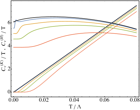
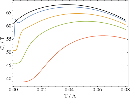
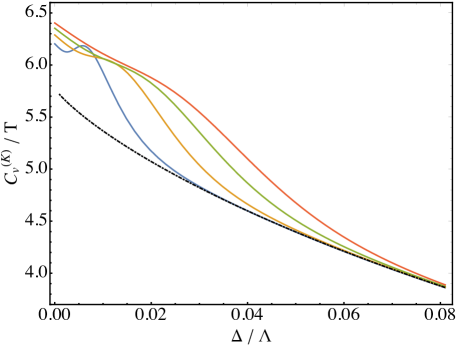
Figure 1: Specific heat contributions $C_{v}^{(H)}/T$ and $C_{v}^{(K)}/T$, evaluated from (III.5.1). Everywhere $\varkappa=1/\Lambda$. (a) and (b) as a function of $T$ at fixed $\Delta$. Black, blue, orange, green and red correspond to $\Delta/\Lambda=\{0,0.5,2,4,8\}\times 10^{-2}$. In (a) solid and dashed lines correspond to $C_{v}^{(K)}/T$ and $C_{v}^{(H)}/T$, and for presentation we take $K=1$. In (b) both contributions are summed $C_{v}/T=C_{v}^{(H)}/T+C_{v}^{(K)}/T$, and we take $K=10$. (c) $C_{v}^{(K)}/T$ as a function of $\Delta$ and fixed $T$: Blue, orange, green and red correspond to $T/\Lambda=\{0.25,0.5,0.75,1.0\}\times 10^{-2}$. The black dot-dashed line corresponds to the asymptotic form obtained for the Fermi liquid regime in (59). (d) $C_{v}/T$ vs $T/\Delta(g)$, with $K=10$. Same color scheme as in (a) and (b).

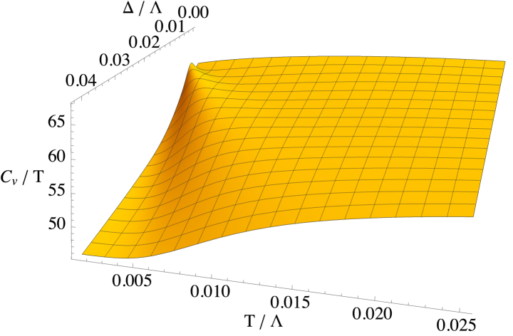
Figure 2: Specific heat surface plot, $C_{v}/T=C_{v}^{(H)}/T+C_{v}^{(K)}/T$ versus $T/\Lambda$ and $\Delta/\Lambda$, with $K=10$.

III.5 Numerical solution

We now turn to a numerical evaluation of the free energy and specific heat in the $K$-expansion, and an evaluation of the Greens function and decoupling fields in the self-consistent theory, i.e. to all orders in $K$.

III.5.1 First order in $K$

Within the $K$-expansion, we focus on the features of the specific heat $C_{v}/T=C_{v}^{(H)}/T+C_{v}^{(K)}/T$, coming from the free energy contributions $F=F_{H}+F_{K}$, with $F_{H}$ in (50) and $F_{K}$ in (53). However, we reshuffle such that all $K$ dependence is collected into $C_{v}^{(K)}/T$, which is achieved via

$$C_{v}^{(H)}/T \equiv-\frac{\partial^{2}}{\partial T^{2}}\left[F_{H}+\frac{[\Delta(T)]^{2}}{2g_{c}^{1}}\right],$$

$$C_{v}^{(K)}/T \equiv-\frac{\partial^{2}}{\partial T^{2}}\left[F_{K}-\frac{[\Delta(T)]^{2}}{2g_{c}^{1}}\right].$$ (60)

For the evaluation, we take $\varkappa=1/\Lambda$, which requires we use the full expression for $g_{c}^{1}$ presented in (78). The temperature dependence of $\Delta(T)$ is obtained from (45).

Figure 1(a) and (b) looks at the relative and combined contributions of $C_{v}^{(H)}/T$ and $C_{v}^{(K)}/T$, as a function of $T$ at fixed $\Delta$. We see a non-monotonic dependence in $C_{v}/T$, coming from the contribution $C_{v}^{(K)}/T$, with a peak at a value $T\sim\Delta$ – this is further manifest in Figure 1(d). Such a peak indicates the change of regime from Fermi liquid $\Delta\gg T$ to quantum critical $\Delta\ll T$, and as such could be a useful experimental Loram et al. (2001); Michon et al. (2019); Tallon et al. (2019) diagnostic of the critical point. In Figure 1(c) we plot $C_{v}^{(K)}/T$ versus $\Delta$ at fixed $T$, which demonstrates a significant conclusion of the present analysis; that upon tuning to the critical point $\Delta\to 0$, $\lim_{T\rightarrow 0}C_{v}^{(K)}/T$ (and hence $\lim_{T\rightarrow 0}C_{v}/T$) is enhanced. Figure 2 provides a surface plot of $C_{v}/T$ versus $T$ and $\Delta$, with fixed $K=10$.

III.5.2 All orders in $K$

We now present aspects of the theory obtained to all orders in $K$; namely the full bosonic mass gap $\Delta(1/g,K,T)$, Greens function $G(\tau)$, and the saddle point of the bilocal field, i.e. $C(\tau)$ and its Fourier transform $\tilde{C}(\omega_{n})$.

For the sake of a self-consistent numerical treatment, the Pauli-Villars procedure is ideal because it does not introduce any sharp cutoffs. Because we also need to regulate the free energy with the same procedure, we choose two subtractions:

$$\tilde{G}(k,\omega_{n})=\frac{1}{k^{2}+\Sigma(\omega_{n})}+\frac{1}{k^{2}+\Sigma(\omega_{n})+2\Lambda^{2}}-\frac{2}{k^{2}+\Sigma(\omega_{n})+\Lambda^{2}}\,.$$ (61)

where we have defined

$$\Sigma(\omega_{n})\equiv\omega_{n}^{2}+\Delta^{2}-2\tilde{C}(\omega_{n})+2\tilde{C}(0)\,.$$ (62)

This ensures a $\sim(k^{2}+\Sigma(\omega_{n}))^{-3}$ decay at large $k$ and $\omega_{n}$.

For the free energy, the corresponding regularization is

$$\int^{\Lambda}\frac{d^{2}k}{4\pi^{2}}\ln\bigl{[}k^{2}+\Sigma(\omega_{n})\bigr{]}=$$

$$~{}~{}~{}\int\frac{d^{2}k}{4\pi^{2}}\Bigr{[}\ln\bigl{[}k^{2}+\Sigma(\omega_{n})\bigr{]}+\ln\bigl{[}k^{2}+\Sigma(\omega_{n})+2\Lambda^{2}\bigr{]}-2\ln\bigl{[}k^{2}+\Sigma(\omega_{n})+\Lambda^{2}\bigr{]}\Bigr{]}$$ (63)

where the right-hand-side decays as $\sim(k^{2}+\Sigma(\omega_{n}))^{-2}$ at large $k$ and $\omega_{n}$, and the saddle point equations of the free energy yield (61). The $k$ integration is readily performed, and upon applying this regularization scheme to the free energy (15), the corresponding saddle point equations (16) and (17) become,

$$C(\tau) = J_{f}(\tau)\frac{T}{4\pi}\sum_{\omega_{n}}e^{-i\omega_{n}\tau}\ln\left[\frac{[\Sigma(\omega_{n})+\Lambda^{2}]^{2}}{\Sigma(\omega_{n})[\Sigma(\omega_{n})+2\Lambda^{2}]}\right]$$ (64)

$$\frac{1}{g} = \frac{T}{4\pi}\sum_{\omega_{n}}\ln\left[\frac{[\Sigma(\omega_{n})+\Lambda^{2}]^{2}}{\Sigma(\omega_{n})[\Sigma(\omega_{n})+2\Lambda^{2}]}\right].$$ (65)

We provide the numerical solution of these saddle point equations in Figure 3. There our focus is on the critical coupling $g=g_{c}$, as well as one value of $g>g_{c}$, chosen such that $\Delta(T=0)/\Lambda=2\times 10^{-3}$. Having these two values of $g$ allows us to tease out the key qualitative features of the saddle point solutions. Figure 3(a) shows the mass gap as a function of $T$. The $g=g_{c}$ results are consistent with log correction obtained analytically in (40). Figure 3(b) and (c) test the logarithmically violated scaling in (42), and show the non-linear influence of $K$ on $C(\tau)$ and $G(\tau)$ – from the ‘large’ time $\tau T\to 1/2$ asymptotic, we see that in the critical case $g=g_{c}$, the deviation from linearity in $K$ is likely only as weak as logarithmic in $K$. These figures also show the expected suppression of these functions for the case $g>g_{c}$, relative to the critical case $g=g_{c}$, which becomes especially pronounced at ‘large’ times, $\tau T\to 1/2$. Finally, in Figure 3(d) we show the frequency space behaviour of $\delta\tilde{C}(\omega_{n})=2\tilde{C}(0)-2\tilde{C}(\omega_{n})$.

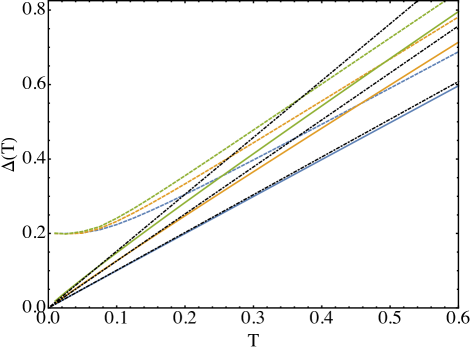
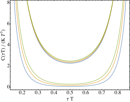
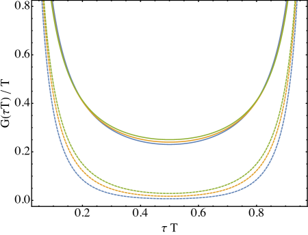
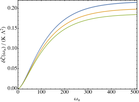
Figure 3: Self-consistent saddle point solutions – Blue, orange, green correspond to $K=\{0.01,0.1,1\}$: Solid lines correspond to the quantum critical mass gap $\Delta(T)$ at $g=g_{c}$, while dashed corresponds to $g>g_{c}$ whereby the zero temperature gap $\Delta(T=0)/\Lambda=2\times 10^{-3}$. (a) Inverse spatial correlation length, $\Delta(T,K)\sim\xi_{x}^{-1}$. Dash-dotted black lines correspond to linear in $T$ fits at small $T$, and are merely a guide to the eye. The curves for $\Delta(T)$ at $g=g_{c}$ are consistent with log correction obtained analytically in (40), whereby at larger $K$ we expect larger log corrections. (b) $C(\tau T)/(KT^{3})$ vs $\tau T$, (c) $G(\tau T)/T$ vs $\tau T$, and (d) $\delta\tilde{C}(\omega_{n})/(K\Lambda^{2})$ vs $\omega_{n}$, where $\delta\tilde{C}(\omega_{n})=2\tilde{C}(0)-2\tilde{C}(\omega_{n})$: In all cases $T/\Lambda=0.25\times 10^{-3}$.

IV Renormalization group analysis

This section will explore the nature of the $1/N_{h}$ corrections to the $N_{h}=\infty$ theory presented in Section III. A complete examination of such corrections requires determination of the fluctuation propagator of the bilocal field $C(x,\tau,\tau^{\prime})$. Rather than undertake this complex task, in this paper we will limit ourselves to a renormalization group (RG) analysis in powers of $K$ within the large $N_{h}$ expansion. We will be performing a double expansion in powers of $K$ and $1/N_{h}$, with $K\sim 1/N_{h}$.

Figure 4: Diagrams for the RG computation. (a) Propagator of $D_{\ell m}$. (b) Propagator for $H_{a\ell}$ (c) Interaction vertex between $D_{\ell m}$ and $H_{a\ell}$. (d) Self-energy renormalizations for $H_{a\ell}$ at order $K$. (e-i) Self energy diagrams at order $K/N_{h}$; the dotted wavy line is the gauge propagator for $A_{a\mu}$, and the dashed wavy lines represent $B_{0}$ and $B_{1,ab}$ propagators. (j) Vertex renormalization at order $K/N_{h}$. The vertex renormalization at order $1/N_{h}$ was computed in Ref. Sachdev et al., 2019, and is not shown here. We do not compute diagrams (e-j) in this paper, because they are needed to determine the RG fixed point in (74) at order $1/N_{h}$.

To linear order in $K$, the RG equation for $K$ follows from a determination of the scaling dimension of $\mathcal{S}_{f}$ in (5); this was already computed in Ref. Sachdev et al., 2019, and yields

$$\frac{dK}{d\ell}=2(1-\Delta_{Q})K+\mathcal{O}(K^{2})$$ (66)

where $\Delta_{Q}$ is the scaling dimension of the O($N_{h}$) order parameter $Q_{\ell m}$ in (6) at $K=0$; this was computed in Ref. Sachdev et al., 2019 to be

$$\Delta_{Q}=1-\frac{64}{3\pi^{2}N_{h}}+\mathcal{O}(1/N_{h}^{2})\,.$$ (67)

So we see the $K$ is relevant at large, but finite $N_{h}$.

The RG analysis is more easily carried out without using bilocal fields. So instead of decoupling $\mathcal{S}_{f}$ in (5) by the bilocal field $C_{ab}$ in (11), we decouple it by a local field $D_{\ell m}(x,\tau)$ Jian et al. (2020);

$$\mathcal{S}_{f}=\frac{1}{2}\int d^{2}xd\tau d\tau^{\prime}\,D_{\ell m}(x,\tau)G_{f}^{-1}(\tau-\tau^{\prime})D_{\ell m}(x,\tau^{\prime})-\sqrt{\frac{K}{N_{h}}}\int d^{2}xd\tau D_{\ell m}(x,\tau)H_{a\ell}(x,\tau)H_{am}(x,\tau)\,.$$ (68)

Here $G_{f}^{-1}$ is the operator inverse of $G_{f}(\tau)=1/\tau^{2}$. The RG analysis can now be carried out by standard diagrammatic methods, using the Feynman graphs illustrated in Fig. 4. The RG equation (66) contains a term of order $K/N_{h}$. The $H_{a\ell}$ self energy diagram in Fig. 4d contributes to the flow of $K$ at order $K^{2}$, while the diagrams in Fig. 4e-j contribute the flow of $K$ at order $K^{2}/N_{h}$. It will be sufficient for our purposes to only compute the diagram in Fig. 4d, which represents the RG implementation of the logarithmic factors discussed in Section III. At external frequency $\omega$, and external momentum $p$, we have

$$\ref{fig:rgdiag}{\rm d}=2K\int\frac{d^{2}k}{4\pi^{2}}\int\frac{d\epsilon}{2\pi}\frac{-\pi|\epsilon|}{[(k+p)^{2}+(\epsilon+\omega)^{2}]}={\rm constant}-K\omega^{2}\int_{\Lambda e^{-\ell}}^{\Lambda}\frac{d^{2}k}{4\pi^{2}}\frac{1}{k^{2}}\,$$ (69)

where $e^{-\ell}$ is the RG rescaling factor. This self energy can be absorbed into rescalings of $x$, $\tau$, and $H_{al}$ via

$$x^{\prime} = xe^{-\ell}$$

$$\tau^{\prime} = \tau e^{-z\ell}$$

$$H_{a\ell}^{\prime} = H_{a\ell}e^{(d+z-2+\eta)\ell/2}\,,$$ (70)

where $z$ is the dynamic critical exponent and $\eta$ is the anomalous dimension of $H_{a\ell}$. From (69) we obtain

$$\eta = 0$$

$$z = 1+\frac{K}{4\pi}\,.$$ (71)

Next, we determine from the first term in (68) that the rescaling of $D_{\ell m}$ is

$$D_{\ell m}^{\prime}=D_{\ell m}e^{(1+z)\ell}\,.$$ (72)

Finally, from the rescalings of the second term in (68), we determine the leading correction to the flow equations in (66) and (67)

$$\frac{dK}{d\ell}=\frac{128}{3\pi^{2}}\frac{K}{N_{h}}-\frac{K^{2}}{2\pi}+\mathcal{O}\left(\frac{K}{N_{h}^{2}},\frac{K^{2}}{N_{h}},K^{3}\right)\,.$$ (73)

The RG flow equation has an infrared stable fixed point at

$$K^{\ast}=\frac{256}{3\pi N_{h}}+\mathcal{O}\left(\frac{1}{N_{h}^{2}}\right).$$ (74)

Note that the relevant direction associated with $g-g_{c}$ is still present at this fixed point, which is our candidate for cuprate criticality. From (71) we obtain the dynamic critical exponent

$$z=1+\frac{64}{3\pi^{2}N_{h}}+\mathcal{O}\left(\frac{1}{N_{h}^{2}}\right)\,.$$ (75)

The field $H_{a\ell}$ is not gauge invariant, and so its anomalous dimension $\eta$ is not well-defined: it can be useful to define a gauge-dependent $\eta$ for intermediate steps in a computation, but it does not directly determine any observable. In (71), we obtained $\eta=0$ to leading order in $K$, but we have not explicitly included a wavefunction renormalization from the gauge field. Indeed this wavefunction renormalization is an ingredient Sachdev et al. (2019) in the computation of the anomalous dimension of the gauge-invariant composite operator $Q_{\ell m}$ in (67), which entered our RG flow equation (73).

We turn to the critical behavior of the free energy density. In a theory obeying hyperscaling, we expect $F\sim T^{(d+z)/z}=T^{1+2/z}$. Using the value of $z$ in (71), and expanding in powers of $K$, we obtain $F\sim T^{3}[1+(K/(2\pi))\ln(\bullet)+\ldots]$. We see that this hyperscaling contribution to the free energy perfectly explains the $T^{3}\ln(\bullet)$ terms in $F_{2}$ and $F_{3}$ in Appendix B.

V Conclusions

We have analyzed a model of optimal doping criticality in the cuprates Sachdev et al. (2019); Scammell et al. (2020). The underlying transition is a Higgs-confinement transition in a SU(2) gauge theory, with the Higgs field corresponding to the spin density wave order in a rotating frame of reference. The Higgs field transforms as an adjoint of the emergent SU(2) gauge field, and so is not directly observable. However, gauge-invariant composites of the Higgs field can break symmetries associated with charge density wave, Ising-nematic, and time-reversal odd scalar spin chirality orders. So the underdoped regime, which corresponds to the Higgs phase, can display one of these orders. In addition, the Higgs condensate need not break the SU(2) gauge symmetry completely, and any unbroken discrete gauge symmetries can lead to bulk topological order with anyonic excitations. The confining phase of the SU(2) gauge theory corresponds to the Fermi liquid in the overdoped regime of the cuprates.

A particularly difficult issue in the treatment of cuprate criticality is the role of the fermions carrying the electromagnetic charge. In many models, these fermions are fractionalized, and also carry emergent gauge charges: then there is a singular renormalization of the fermionic excitations at the Fermi surface, which is difficult to treat in a controlled manner. In the model of Ref. Sachdev et al. (2019) (and also in some earlier models Sachdev and Morinari (2002); Nussinov and Zaanen (2002); Zaanen and Nussinov (2003); Mross and Senthil (2012a, b)), the electromagnetically charged fermions are argued to be electron-like and have a large Fermi surface (whose volume is given by the conventional Luttinger value). We have shown here that a $1/N_{h}$ expansion allows a controlled treatment of the consequences of such a Fermi surface. It leads to a quantum field theory which is bilocal in time, with a strongly-coupled fixed point with dynamic critical exponent $z>1$.

We showed that the critical free energy obeyed hyperscaling. At intermediate stages in our computation, hyperscaling violating terms do appear; however we showed in Section III.4 and Appendix A and B that such terms cancel after accounting for fluctuation corrections to the position of the quantum critical point. The resulting specific heat is described by (1), with a smooth background linear in $T$ specific heat, and a singular hyperscaling preserving contribution. Plots of $C_{v}/T$ as a function of $T$ and $\Delta$ (the Higgs gap, an energy scale measuring distance from the quantum critical point on the overdoped side) are shown in Fig. 1. There is a finite enhancement of the background contribution $\gamma_{b}$, shown as the first term in (59), which can be viewed as an increase in the effective mass of the background fermions from the Higgs fluctuations. The remaining terms in (59), belong to the singular contribution obeying hyperscaling, and show a $\Delta$-dependent finite enhancement in the value $\lim_{T\rightarrow 0}C_{v}/T$ as the critical point is approached with $\Delta$ becoming smaller. At a fixed $\Delta$, we also found a non-monotonic $T$ dependence in $C_{v}/T$ at small $\Delta$, with a peak at a value $T\sim\Delta$. This peak is an indication of a crossover associated with the underlying fluctuations of the Higgs field, and could be a useful experimental Loram et al. (2001); Michon et al. (2019); Tallon et al. (2019) diagnostic of the critical point.

Acknowledgements

We acknowledge useful discussions with Chao-Ming Jian and Cenke Xu. This research was supported by the National Science Foundation under Grant No. DMR-2002850.

Appendix A Position of the critical point

We work at $T=0$ and $g=g_{c}$, when $\Delta(T)=0$, and then the saddle point equations in (16) and (17) become

$$\int^{\Lambda}\frac{d^{2}k}{4\pi^{2}}\int\frac{d\omega}{2\pi}\frac{1}{k^{2}+\omega^{2}-2\tilde{C}(\omega)+2\tilde{C}(0)}=\frac{1}{g_{c}}$$ (76)

$$\tilde{C}(\omega)=\int\frac{d\epsilon}{2\pi}\tilde{J}_{f}(\epsilon+\omega)\int^{\Lambda}\frac{d^{2}k}{4\pi^{2}}\frac{1}{k^{2}+\epsilon^{2}-2\tilde{C}(\epsilon)+2\tilde{C}(0)}$$

We manipulate these equations to obtain the first order correction to $g_{c}^{0}=4\pi/\Lambda$. Keeping only the first order term in $K$ in the second equation in (76) we obtain

$$\tilde{C}(\omega)-\tilde{C}(0)=\int\frac{d\epsilon}{2\pi}\int^{\Lambda}\frac{d^{2}k}{4\pi^{2}}\frac{\left[\tilde{J}_{f}(\epsilon+\omega)-\tilde{J}(\epsilon)\right]}{k^{2}+\epsilon^{2}}$$ (77)

Inserting this back into the first equation in (76) we obtain our needed result for $g_{c}^{1}$ in (46)

$$\frac{1}{g_{c}^{1}}=2\int\frac{d\omega d\epsilon}{4\pi^{2}}\int^{\Lambda}\frac{d^{2}p}{4\pi^{2}}\int^{\Lambda}\frac{d^{2}k}{4\pi^{2}}\frac{\left[\tilde{J}_{f}(\epsilon+\omega)-\tilde{J}(\epsilon)\right]}{(k^{2}+\epsilon^{2})(p^{2}+\omega^{2})^{2}}$$ (78)

We now evaluate these expressions analytically in the limit $\varkappa\rightarrow 0$. From (77)

$$\tilde{C}(\omega)-\tilde{C}(0) = -\pi K\int\frac{d\epsilon}{2\pi}\int^{\Lambda}\frac{d^{2}k}{4\pi^{2}}\frac{\left(|\epsilon+\omega|-|\epsilon|\right)}{k^{2}+\epsilon^{2}}$$ (79)

$$= -\frac{K}{4}\int\frac{d\epsilon}{2\pi}\left(|\epsilon+\omega|-|\epsilon|\right)\ln\left(\frac{\Lambda^{2}+\epsilon^{2}}{\epsilon^{2}}\right)$$

$$= -\frac{K\Lambda\omega}{2\pi}\tan^{-1}\left(\frac{\omega}{\Lambda}\right)+\frac{K\Lambda^{2}}{8\pi}\ln\left(\frac{\Lambda^{2}+\omega^{2}}{\Lambda^{2}}\right)-\frac{K\omega^{2}}{8\pi}\ln\left(\frac{\Lambda^{2}+\omega^{2}}{\omega^{2}}\right)$$

From the first equation in (76), the value of $g_{c}$ is then

$$\frac{1}{g_{c}}=\frac{\Lambda}{4\pi}+\frac{1}{2\pi}\int\frac{d\omega}{2\pi}\left(\frac{1}{\omega^{2}}-\frac{1}{\Lambda^{2}+\omega^{2}}\right)\left(\tilde{C}(\omega)-\tilde{C}(0)\right)\,.$$ (80)

So, evaluating $\omega$ integral

$$\frac{1}{g_{c}^{1}}=-\frac{K\Lambda}{8\pi^{2}}\left(2\ln 2-\frac{1}{2}\right)\,,\quad\mbox{as $\varkappa\rightarrow 0$.}$$ (81)

It is interesting to compare the expressions (78) and (81) with that obtained from the derivative of $F_{K}$ with respect to $T$ starting from the expression in (53) and (54). In taking this derivative, we ignore any $T$ dependence that arises from the Matsubara frequency summation: such terms involve derivatives of Bose functions which vanish exponentially at large argument, and so do not contribute to the ultraviolent divergent term $F_{K}\sim\Lambda[\Delta(T)]^{2}$ we are interested. Furthermore, it is important for our argument that the $T$-dependence of $\Delta(T)$ is compatible with the constraint (17), or more explicitly (93). So we obtain

$$\frac{1}{3N_{h}}\frac{\partial F_{K}}{\partial T}\approx\frac{\partial[\Delta(T)]^{2}}{\partial T}T^{2}\sum_{\omega_{n},\epsilon_{n}}\int^{\Lambda}\frac{d^{2}p}{4\pi^{2}}\int^{\Lambda}\frac{d^{2}k}{(2\pi)^{2}}\tilde{J}_{f}(\epsilon_{n}+\omega_{n})\tilde{G}(k,\epsilon_{n})\tilde{G}^{2}(p,\omega_{n})\,.$$ (82)

Now comparing (82) with (78) we see that the first term in (78) has the same form as (82). The only differences are the frequency integration versus frequency summation, and the presence of the ‘mass’ $[\Delta(T)]^{2}$ in the Green’s function in (82). However, these differences are not important for the ultraviolet $\Lambda$-dependence we are interested in. The second term in (78) is needed to cancel the $1/\omega^{2}$ infrared divergence in the first term. There is no such infrared divergence in (82) because of the $[\Delta(T)]^{2}$ mass in $\tilde{G}$. If we were to add a term corresponding to the second term of (78) to (82), we would have the concern that this introduces additional ultraviolet divergent terms not in $F_{K}$. However, this does not happen because

$$-\frac{\partial[\Delta(T)]^{2}}{\partial T}T^{2}\sum_{\omega_{n},\epsilon_{n}}\int^{\Lambda}\frac{d^{2}p}{4\pi^{2}}\int^{\Lambda}\frac{d^{2}k}{(2\pi)^{2}}\tilde{J}_{f}(\epsilon_{n})\tilde{G}(k,\epsilon_{n})\tilde{G}^{2}(p,\omega_{n})\approx$$ (83)

$$~{}~{}~{}~{}~{}~{}~{}~{}~{}~{}~{}~{}~{}~{}~{}~{}\left[\sum_{\epsilon_{n}}\int^{\Lambda}\frac{d^{2}k}{(2\pi)^{2}}\tilde{J}_{f}(\epsilon_{n})\tilde{G}(k,\epsilon_{n})\right]\frac{\partial}{\partial T}\left[\sum_{\omega_{n}}\int^{\Lambda}\frac{d^{2}p}{(2\pi)^{2}}\tilde{G}(p,\omega_{n})\right]\,$$

vanishes by the constraint equation (17) (up to terms involving derivatives of Bose functions that we are allowed to drop because we are only interested in ultraviolet contributions). Therefore, such a term is not needed, and the correspondence between (82) and (78) is complete without it: this explains why the co-efficient of the term divergent as $\sim\Lambda[\Delta(T)]^{2}$ in (58) matches (50) and (81). The constraint equation (17) was crucial for this argument, as it was in evaluating $F_{K}$ to obtain (58) in Appendix B.

Appendix B Evaluation of free energy terms proportional to $K$

This appendix describes the evaluation of the integrals in (III.4.2). We will split (III.4.2) into various contributions, and take the limit $\kappa\rightarrow 0$

$$F_{K}=F_{1}+F_{2}+F_{3}$$ (84)

The $F_{1}$ contribution arises from the first two terms in (III.4.2); expanding in $\varkappa$ and using (48,51) we obtain

$$\frac{F_{1}}{3N_{h}} = -\frac{K}{32\pi\varkappa}\int_{\Delta(T)}^{\sqrt{\Lambda^{2}+[\Delta(T)]^{2}}}da\int_{\Delta(T)}^{\sqrt{\Lambda^{2}+[\Delta(T)]^{2}}}db(1+2n(a))(1+2n(b))+\mathcal{O}(\varkappa)$$ (85)

$$= -\frac{\pi K}{2\varkappa g_{R}^{2}}+\mathcal{O}(\varkappa)$$

Using (48) we can write

$$\frac{\Delta}{4\pi}-\frac{\sqrt{\Lambda^{2}+\Delta^{2}}-\Lambda}{4\pi}=\frac{\Delta}{4\pi}-\frac{\Delta^{2}}{8\pi\Lambda}+\ldots=\frac{1}{g_{c}^{0}}-\frac{1}{g_{R}}\,,$$ (86)

and so

$$\frac{F_{1}}{3N_{h}}=-\frac{K}{32\pi\varkappa}\left(\sqrt{\Lambda^{2}+\Delta^{2}}-\Delta\right)^{2}+\mathcal{O}(\varkappa)$$ (87)

So $F_{1}$ is $T$-independent, and a smooth function of $\Delta$.

The $F_{2}$ contribution arises from the last two terms in (III.4.2), but without the $n(\Omega)$ factor. Performing the $\Omega$ integral, we obtain

$$\frac{F_{2}}{3N_{h}} = -\frac{K}{16\pi^{2}}\int_{\Delta(T)}^{\sqrt{\Lambda^{2}+[\Delta(T)]^{2}}}da\int_{\Delta(T)}^{\sqrt{\Lambda^{2}+[\Delta(T)]^{2}}}db\Biggl{[}\ln(\varkappa)\left[a(1+2n(b))+b(1+2n(a))\right]$$ (88)

$$~{}~{}~{}~{}~{}~{}+\ln(|a-b|)(b-a)(n(a)-n(b))+\ln(|a+b|)(b+a)(1+n(a)+n(b))\Biggr{]}$$

$$= -\frac{K\Lambda^{2}}{4\pi g_{R}}\ln(\varkappa)-\frac{K}{16\pi^{2}}\int_{\Delta(T)}^{\sqrt{\Lambda^{2}+[\Delta(T)]^{2}}}da\int_{\Delta(T)}^{\sqrt{\Lambda^{2}+[\Delta(T)]^{2}}}db\Biggl{[}$$

$$~{}~{}~{}~{}~{}~{}+\ln(|a-b|)(b-a)(n(a)-n(b))+\ln(|a+b|)(b+a)(1+n(a)+n(b))\Biggr{]}$$

Finally, the $F_{3}$ contribution arises from the terms containing the $n(\Omega)$ factor in the last two terms in (III.4.2)

$$\frac{F_{3}}{3N_{h}} = -\frac{1}{16\pi^{2}}\int_{\Delta(T)}^{\sqrt{\Lambda^{2}+[\Delta(T)]^{2}}}da\int_{\Delta(T)}^{\sqrt{\Lambda^{2}+[\Delta(T)]^{2}}}db\Biggl{[}$$ (89)

$$~{}~{}~{}~{}~{}~{}~{}+2K\int_{0}^{\infty}d\Omega\,\Omega n(\Omega)\,\mathcal{P}\left(\frac{1}{(a-b)^{2}-\Omega^{2}}\right)(b-a)(n(a)-n(b))$$

$$~{}~{}~{}~{}~{}~{}~{}+2K\int_{0}^{\infty}d\Omega\,\Omega n(\Omega)\,\mathcal{P}\left(\frac{1}{(a+b)^{2}-\Omega^{2}}\right)(a+b)(1+n(a)+n(b))\Biggr{]}\,.$$

So far, the manipulations have been exact. Now we will evaluate the integrals while dropping terms which scale as $T^{3}\ln(\bullet)$ and are exponentially small in the regime $T\ll\Delta$.

The case of $F_{3}$ is simpler, so we consider it first. In the stated approximation, the only significant contribution in (89) is

$$\frac{F_{3}}{3N_{h}} \approx -\frac{K}{8\pi^{2}}\left[\int_{0}^{\infty}d\Omega\,\Omega n(\Omega)\right]\int_{\Delta}^{\sqrt{\Lambda^{2}+\Delta^{2}}}da\int_{\Delta}^{\sqrt{\Lambda^{2}+\Delta^{2}}}db\,\frac{1}{a+b}$$ (90)

$$= -\frac{KT^{2}}{24}\left[\Lambda\ln(2)-\Delta\ln\left(\frac{\Lambda}{2\Delta}\right)-\Delta\right]$$

Finally, let us turn to the evaluation of $F_{2}$. After interchanging the $a$ and $b$ integrands in (88) so that all the Bose functions are $n(a)$, the $b$ integration can be performed exactly, and we obtain

$$\frac{F_{2}}{3N_{h}} = -\frac{K\Lambda^{2}}{4\pi g_{R}}\ln(\varkappa)-\frac{K}{16\pi^{2}}\int_{\Delta(T)}^{\sqrt{\Lambda^{2}+[\Delta(T)]^{2}}}da\Biggl{[}-n(a)\left(a-\Delta(T)\right)^{2}\left(\ln\left(a-\Delta(T)\right)-\frac{1}{2}\right)$$ (91)

$$~{}~{}~{}~{}~{}~{}\,+n(a)\left(\sqrt{\Lambda^{2}+[\Delta(T)]^{2}}-a\right)^{2}\left(\ln\left(\sqrt{\Lambda^{2}+[\Delta(T)]^{2}}-a\right)-\frac{1}{2}\right)$$

$$~{}~{}~{}~{}~{}~{}+(n(a)+1/2)\left(\sqrt{\Lambda^{2}+[\Delta(T)]^{2}}+a\right)^{2}\left(\ln\left(\sqrt{\Lambda^{2}+[\Delta(T)]^{2}}+a\right)-\frac{1}{2}\right)$$

$$~{}~{}~{}~{}~{}~{}-(n(a)+1/2)\left(a+\Delta(T)\right)^{2}\left(\ln\left(a+\Delta(T)\right)-\frac{1}{2}\right)\Biggr{]}\,.$$

Now we make the approximation described above, of dropping terms which scale as $T^{3}\ln(\bullet)$ and are exponentially small for $T\ll\Delta$; then some of the integrals can be evaluated:

$$\frac{F_{2}}{3N_{h}} \approx -\frac{K\Lambda^{2}}{4\pi g_{R}}\ln(\varkappa)-\frac{K}{16\pi^{2}}\Lambda^{2}(2\ln\Lambda-1)\int_{\Delta(T)}^{\infty}da\,n(a)-\frac{K}{16\pi^{2}}\int_{\Delta(T)}^{\sqrt{\Lambda^{2}+[\Delta(T)]^{2}}}da\Biggl{[}$$ (92)

$$~{}~{}~{}~{}~{}~{}\,+(1/2)\left(\sqrt{\Lambda^{2}+[\Delta(T)]^{2}}+a\right)^{2}\left(\ln\left(\sqrt{\Lambda^{2}+[\Delta(T)]^{2}}+a\right)-\frac{1}{2}\right)$$

$$~{}~{}~{}~{}~{}~{}-(1/2)\left(a+\Delta(T)\right)^{2}\left(\ln\left(a+\Delta(T)\right)-\frac{1}{2}\right)\Biggr{]}$$

$$= -\frac{K\Lambda^{3}}{16\pi^{2}}\left[\ln(\varkappa\Lambda)+\frac{4}{3}\ln 2-\frac{5}{6}\right]+\frac{K\Lambda^{2}\Delta}{16\pi^{2}}\left(1-\frac{\Delta}{2\Lambda}\right)\ln(\varkappa)-\frac{K}{16\pi^{2}}\Biggl{[}-\frac{\Delta(T)\Lambda^{2}}{2}(2\ln\Lambda-1)$$

$$~{}~{}~{}~{}~{}~{}~{}+\frac{[\Delta(T)]^{2}\Lambda}{4}\left(-3+8\ln 2+2\ln\Lambda\right)+\Lambda^{2}(2\ln\Lambda-1)\int_{\Delta(T)}^{\infty}da\,n(a)\Biggr{]}\,.$$

In (92), we have used an expression for $g_{R}$ that follow from the constraint equations (48,51) which we write as

$$\int_{\Delta(T)}^{\sqrt{\Lambda^{2}+[\Delta(T)]^{2}}}da(1+2n(a))=\frac{4\pi}{g_{R}}\,.$$ (93)

We also used (86) to express $g_{R}$ in terms $\Lambda$ and $\Delta$. We can also use (93) and (86) to write

$$\int_{\Delta(T)}^{\infty}da\,n(a)=\frac{\Delta(T)-\Delta}{2}-\frac{[\Delta(T)]^{2}-\Delta^{2}}{4\Lambda}+\ldots\,.$$ (94)

Now inserting (94) in (92), we obtain

$$\frac{F_{2}}{3N_{h}} \approx -\frac{K\Lambda^{3}}{16\pi^{2}}\left[\ln(\varkappa\Lambda)+\frac{4}{3}\ln 2-\frac{5}{6}\right]+\frac{K\Lambda^{2}\Delta}{16\pi^{2}}\left(1-\frac{\Delta}{2\Lambda}\right)\left[\ln(\varkappa\Lambda)-\frac{1}{2}\right]$$ (95)

$$~{}~{}-\frac{K\Lambda[\Delta(T)]^{2}}{16\pi^{2}}\Biggl{[}2\ln 2-\frac{1}{2}\Biggr{]}\,.$$

It is notable that all terms of order $\Delta\Lambda^{2}\ln\Lambda$, $\Delta\Lambda^{2}$, and $\Delta^{2}\Lambda\ln\Lambda$ cancel, even though they appear at intermediate orders. This is related to use of the constraint (17), and the discussion in the latter part of Appendix A.

References

- Proust and Taillefer (2019) C. Proust and L. Taillefer, “The Remarkable Underlying Ground States of Cuprate Superconductors,” Annual Review of Condensed Matter Physics 10, 409 (2019), arXiv:1807.05074 [cond-mat.supr-con] .
- Vishik et al. (2012) I. M. Vishik, M. Hashimoto, R.-H. He, W.-S. Lee, F. Schmitt, D. Lu, R. G. Moore, C. Zhang, W. Meevasana, T. Sasagawa, S. Uchida, K. Fujita, S. Ishida, M. Ishikado, Y. Yoshida, H. Eisaki, Z. Hussain, T. P. Devereaux, and Z.-X. Shen, “Phase competition in trisected superconducting dome,” Proceedings of the National Academy of Science 109, 18332 (2012), arXiv:1209.6514 [cond-mat.supr-con] .
- He et al. (2014) Y. He, Y. Yin, M. Zech, A. Soumyanarayanan, M. M. Yee, T. Williams, M. C. Boyer, K. Chatterjee, W. D. Wise, I. Zeljkovic, T. Kondo, T. Takeuchi, H. Ikuta, P. Mistark, R. S. Markiewicz, A. Bansil, S. Sachdev, E. W. Hudson, and J. E. Hoffman, “Fermi Surface and Pseudogap Evolution in a Cuprate Superconductor,” Science 344, 608 (2014), arXiv:1305.2778 [cond-mat.supr-con] .
- Fujita et al. (2014) K. Fujita, C. K. Kim, I. Lee, J. Lee, M. H. Hamidian, I. A. Firmo, S. Mukhopadhyay, H. Eisaki, S. Uchida, M. J. Lawler, E.-A. Kim, and J. C. Davis, “Simultaneous Transitions in Cuprate Momentum-Space Topology and Electronic Symmetry Breaking,” Science 344, 612 (2014), arXiv:1403.7788 [cond-mat.supr-con] .
- Badoux et al. (2016) S. Badoux, W. Tabis, F. Laliberté, G. Grissonnanche, B. Vignolle, D. Vignolles, J. Béard, D. A. Bonn, W. N. Hardy, R. Liang, N. Doiron-Leyraud, L. Taillefer, and C. Proust, “Change of carrier density at the pseudogap critical point of a cuprate superconductor,” Nature 531, 210 (2016), arXiv:1511.08162 [cond-mat.supr-con] .
- Loram et al. (2001) J. Loram, J. Luo, J. Cooper, W. Liang, and J. Tallon, “Evidence on the pseudogap and condensate from the electronic specific heat,” Journal of Physics and Chemistry of Solids 62, 59 (2001).
- Michon et al. (2019) B. Michon, C. Girod, S. Badoux, J. Kačmarčík, Q. Ma, M. Dragomir, H. A. Dabkowska, B. D. Gaulin, J. S. Zhou, S. Pyon, T. Takayama, H. Takagi, S. Verret, N. Doiron-Leyraud, C. Marcenat, L. Taillefer, and T. Klein, “Thermodynamic signatures of quantum criticality in cuprate superconductors,” Nature 567, 218 (2019), arXiv:1804.08502 [cond-mat.supr-con] .
- Tallon et al. (2019) J. L. Tallon, J. G. Storey, J. R. Cooper, and J. W. Loram, “Locating the pseudogap closing point in cuprate superconductors: absence of entrant or reentrant behavior,” (2019), arXiv:1907.12018 [cond-mat.supr-con] .
- Tang et al. (2018) Y. Tang, L. Mangin-Thro, A. Wildes, M. K. Chan, C. J. Dorow, J. Jeong, Y. Sidis, M. Greven, and P. Bourges, “Orientation of the intra-unit-cell magnetic moment in the high- superconductor HgBa2CuO4+δ,” Phys. Rev. B 98, 214418 (2018), arXiv:1805.02063 [cond-mat.supr-con] .
- Chen et al. (2019) S.-D. Chen, M. Hashimoto, Y. He, D. Song, K.-J. Xu, J.-F. He, T. P. Devereaux, H. Eisaki, D.-H. Lu, J. Zaanen, and Z.-X. Shen, “Incoherent strange metal sharply bounded by a critical doping in Bi2212,” Science 366, 1099 (2019).
- Panagopoulos et al. (2002) C. Panagopoulos, J. L. Tallon, B. D. Rainford, T. Xiang, J. R. Cooper, and C. A. Scott, “Evidence for a generic quantum transition in high- cuprates,” Phys. Rev. B 66, 064501 (2002), arXiv:cond-mat/0204106 [cond-mat.supr-con] .
- Panagopoulos et al. (2004) C. Panagopoulos, A. P. Petrovic, A. D. Hillier, J. L. Tallon, C. A. Scott, and B. D. Rainford, “Exposing the spin-glass ground state of the nonsuperconducting La2-xSrxCu1-yZnyO4 high- oxide,” Phys. Rev. B 69, 144510 (2004), arXiv:cond-mat/0307392 [cond-mat.supr-con] .
- Frachet et al. (2019) M. Frachet, I. Vinograd, R. Zhou, S. Benhabib, S. Wu, H. Mayaffre, S. Krämer, S. K. Ramakrishna, A. Reyes, J. Debray, T. Kurosawa, N. Momono, M. Oda, S. Komiya, S. Ono, M. Horio, J. Chang, C. Proust, D. LeBoeuf, and M.-H. Julien, “Hidden magnetism at the pseudogap critical point of a high temperature superconductor,” (2019), arXiv:1909.10258 [cond-mat.supr-con] .
- Sachdev et al. (2019) S. Sachdev, H. D. Scammell, M. S. Scheurer, and G. Tarnopolsky, “Gauge theory for the cuprates near optimal doping,” Phys. Rev. B 99, 054516 (2019), arXiv:1811.04930 [cond-mat.str-el] .
- Scammell et al. (2020) H. D. Scammell, K. Patekar, M. S. Scheurer, and S. Sachdev, “Phases of SU(2) gauge theory with multiple adjoint Higgs fields in 2+1 dimensions,” Phys. Rev. B 101, 205124 (2020), arXiv:1912.06108 [cond-mat.str-el] .
- Sachdev and Morinari (2002) S. Sachdev and T. Morinari, “Strongly coupled quantum criticality with a Fermi surface in two dimensions: Fractionalization of spin and charge collective modes,” Phys. Rev. B 66, 235117 (2002), arXiv:cond-mat/0207167 [cond-mat.str-el] .
- Nussinov and Zaanen (2002) Z. Nussinov and J. Zaanen, “Stripe fractionalization I: the generation of Ising local symmetry,” J. Phys. IV France 12, 245 (2002), cond-mat/0209437 .
- Zaanen and Nussinov (2003) J. Zaanen and Z. Nussinov, “Stripe fractionalization: the quantum spin nematic and the Abrikosov lattice,” Phys. Stat. Sol. B 236, 332 (2003), cond-mat/0209441 .
- Grover and Senthil (2010) T. Grover and T. Senthil, “Quantum phase transition from an antiferromagnet to a spin liquid in a metal,” Phys. Rev. B 81, 205102 (2010), arXiv:0910.1277 [cond-mat.str-el] .
- Kaul et al. (2008) R. K. Kaul, M. A. Metlitski, S. Sachdev, and C. Xu, “Destruction of Néel order in the cuprates by electron doping,” Phys. Rev. B 78, 045110 (2008), arXiv:0804.1794 [cond-mat.str-el] .
- Mross and Senthil (2012a) D. F. Mross and T. Senthil, “Theory of a Continuous Stripe Melting Transition in a Two-Dimensional Metal: A Possible Application to Cuprate Superconductors,” Phys. Rev. Lett. 108, 267001 (2012a), arXiv:1201.3358 [cond-mat.str-el] .
- Mross and Senthil (2012b) D. F. Mross and T. Senthil, “Stripe melting and quantum criticality in correlated metals,” Phys. Rev. B 86, 115138 (2012b), arXiv:1207.1442 [cond-mat.str-el] .
- Hertz (1976) J. A. Hertz, “Quantum critical phenomena,” Phys. Rev. B 14, 1165 (1976).
- Read et al. (1995) N. Read, S. Sachdev, and J. Ye, “Landau theory of quantum spin glasses of rotors and Ising spins,” Phys. Rev. B 52, 384 (1995), arXiv:cond-mat/9412032 [cond-mat] .
- Georges et al. (2000) A. Georges, O. Parcollet, and S. Sachdev, “Mean Field Theory of a Quantum Heisenberg Spin Glass,” Phys. Rev. Lett. 85, 840 (2000), cond-mat/9909239 .
- Georges et al. (2001) A. Georges, O. Parcollet, and S. Sachdev, “Quantum fluctuations of a nearly critical Heisenberg spin glass,” Phys. Rev. B 63, 134406 (2001), cond-mat/0009388 .
- Maldacena and Stanford (2016) J. Maldacena and D. Stanford, “Remarks on the Sachdev-Ye-Kitaev model,” Phys. Rev. D 94, 106002 (2016), arXiv:1604.07818 [hep-th] .
- Kitaev and Suh (2018) A. Kitaev and S. J. Suh, “The soft mode in the Sachdev-Ye-Kitaev model and its gravity dual,” JHEP 05, 183 (2018), arXiv:1711.08467 [hep-th] .
- Gu et al. (2020) Y. Gu, A. Kitaev, S. Sachdev, and G. Tarnopolsky, “Notes on the complex Sachdev-Ye-Kitaev model,” JHEP 02, 157 (2020), arXiv:1910.14099 [hep-th] .
- Chubukov et al. (1994) A. V. Chubukov, S. Sachdev, and J. Ye, “Theory of two-dimensional quantum heisenberg antiferromagnets with a nearly critical ground state,” Phys. Rev. B 49, 11919 (1994).
- Podolsky and Sachdev (2012) D. Podolsky and S. Sachdev, “Spectral functions of the Higgs mode near two-dimensional quantum critical points,” Phys. Rev. B 86, 054508 (2012), arXiv:1205.2700 [cond-mat.quant-gas] .
- Amit (1984) D. Amit, Field Theory, the Renormalization Group, and Critical Phenomena, International Series in Pure and Applied Physics (World Scientific, 1984).
- Jian et al. (2020) C.-M. Jian, Y. Xu, X.-C. Wu, and C. Xu, “Continuous Néel-VBS Quantum Phase Transition in Non-Local one-dimensional systems with SO(3) Symmetry,” (2020), arXiv:2004.07852 [cond-mat.str-el] .