Robust Decoding from Binary Measurements with Cardinality Constraint Least Squares

Abstract

The main goal of 1-bit compressive sampling is to decode $n$ dimensional signals with sparsity level $s$ from $m$ binary measurements. This is a challenging task due to the presence of nonlinearity, noises and sign flips. In this paper, the cardinality constraint least square is proposed as a desired decoder. We prove that, up to a constant $c$, with high probability, the proposed decoder achieves a minimax estimation error as long as $m\geq\mathcal{O}(s\log n)$. Computationally, we utilize a generalized Newton algorithm (GNA) to solve the cardinality constraint minimization problem with the cost of solving a least squares problem with small size at each iteration. We prove that, with high probability, the $\ell_{\infty}$ norm of the estimation error between the output of GNA and the underlying target decays to $\mathcal{O}(\sqrt{\frac{\log n}{m}})$ after at most $\mathcal{O}(\log s)$ iterations. Moreover, the underlying support can be recovered with high probability in $\mathcal{O}(\log s)$ steps provided that the target signal is detectable. Extensive numerical simulations and comparisons with state-of-the-art methods are presented to illustrate the robustness of our proposed decoder and the efficiency of the GNA algorithm.
Keywords: 1-bit compressive sampling, least square with cardinality constraint, minimax estimation error, generalized Newton algorithm, support recovery.

1 Introduction

Compressive sensing is a powerful signal acquisition approach with which one can recover signals beyond bandlimitedness from noisy under-determined measurements whose number is closer to the order of the signal complexity than the Nyquist rate [9, 11, 12, 14]. Quantization that transforms the infinite-precision measurements into discrete ones is necessary for storage and transmission [37]. Among others, scalar quantization is widely considered due to its low computational complexity. A scalar quantizer $\mathcal{Q}(\cdot)$ with bit depth $b$ is fully characterized by the quantization regions $\{[r_{\ell},r_{\ell+1})\}_{\ell=1}^{L}$ constituting a partition of $\mathbb{R}$, where $L=2^{b}$, $r_{1}=-\infty,\ \ r_{L+1}=\infty$ as well as the codebook $\{\omega_{\ell}\}_{\ell=1}^{L}$, where $\mathcal{Q}(t)=\omega_{\ell}$ if $t\in[r_{\ell},r_{\ell+1})$. The 1-bit quantizer $\mathcal{Q}(t)=\mathrm{sign}(t)$, an extreme case of scalar quantization, that codes the measurements into binary values with a single bit has been introduced into compressed sensing [7]. The 1-bit compressed sensing (1-bit CS) has drawn much attention because of its low cost in hardware implementation and storage and its robustness in the low signal-to-noise ratio scenario [26].

1.1 Notation and 1-bit CS model

We denote by $\Psi_{i}\in\mathbb{R}^{m\times 1},i=1,...,n,$ and $\psi_{j}\in\mathbb{R}^{n\times 1},j=1,...m,$ the $i$th column and $j$th row of $\Psi$, respectively. We denote zero vector by 0. We use $[n]$ to denote the set $\{1,...,n\}$, and $\textbf{I}_{n}$ to denote the identity matrix of size $n\times n$. For $A,B\subseteq[n]$ with cardinality $|A|,|B|$, $x_{A}=(x_{i},i\in A)\in\mathbb{R}^{|A|}$, $\Psi_{A}=(\Psi_{i},i\in A)\in\mathbb{R}^{m\times|A|}$ and $\Psi_{AB}\in\mathbb{R}^{|A|\times|B|}$ denotes a submatrix of $\Psi$ whose rows and columns are listed in $A$ and $B$, respectively. Let ${x|_{A}}=(x_{i}\mathbf{1}_{i\in A})\in\mathbb{R}^{n}$, where, $\mathbf{1}_{A}$ denotes the indicator function of set $A$. Let $|x|_{s,\infty}$ and $|x|_{\mathrm{\min}}$ be the $s$th largest elements (in absolute value) and the minimum absolute value of $x$, respectively. We use $\mathcal{N}(\textbf{0},\Sigma)$ to denote the multivariate normal distribution, with $\Sigma$ symmetric and positive definite. Let $\gamma_{\textrm{max}}(\Sigma)$ and $\gamma_{\textrm{min}}(\Sigma)$ be the largest and the smallest eigenvalues of $\Sigma$, respectively. Let $\mathrm{supp}(x)$ denote the support of $x$. We use $\|x\|_{\Sigma}$ to denote the elliptic norm of $x$ with respect to $\Sigma$, i.e., $\|x\|_{\Sigma}=(x^{t}\Sigma x)^{\frac{1}{2}}.$ Let $\|x\|_{p}=(\sum_{i=1}^{n}|x_{i}|^{p})^{1/p},p\in[1,\infty],$ be the $\ell_{p}$-norm of $x$. We denote the number of nonzero elements of $x$ by $\|x\|_{0}$. The symbols $\|\Psi\|$ and $\|\Psi\|_{\infty}$ stands for the operator norm of $\Psi$ induced by $\ell_{2}$ norm and the maximum pointwise absolute value of $\Psi$, respectively. $\textrm{sign}(\cdot)$ operates componentwise with $\textrm{sign}(z)=1$ if $z\geq 0$ and $\textrm{sign}(z)=-1$ otherwise, and $\odot$ denotes the pointwise Hardmard product. By $\mathcal{O}(\cdot)$, we ignore some positive numerical constants.

Following [32, 20], we consider 1-bit CS model

$$y=\eta\odot\textrm{sign}(\Psi x^{*}+\epsilon),$$ (1)

where $y\in\mathbb{R}^{m}$ are the binary measurements, $x^{*}\in\mathbb{R}^{n}$ is an unknown signal with $\|x^{*}\|_{0}\leq s$, $\Psi\in\mathbb{R}^{m\times n}$ is a random matrix whose rows $\psi_{i},i\in[m]$ are i.i.d. random vectors sampled from $\mathcal{N}(\textbf{0},\Sigma)$ with an unknown covariance matrix $\Sigma$, $\eta\in\mathbb{R}^{m}$ is a random vector modeling the sign flips of $y$ whose coordinates $\eta_{i}s$ are i.i.d. satisfying $\mathbb{P}[\eta_{i}=1]=1-\mathbb{P}[\eta_{i}=-1]=p\neq\frac{1}{2},$ and $\epsilon\in\mathbb{R}^{n}$ is a random vector sampled from $\mathcal{N}(\textbf{0},\sigma^{2}\textbf{I}_{m})$ with an unknown noise level $\sigma$ modeling errors before quantization. We assume $\eta_{i},\epsilon_{i}$ and $\psi_{i}$ are independent. Since $\sigma$ is unknown, model (1) is unidentifiable in the sense that $y=\eta\odot\textrm{sign}(\Psi x^{*}+\epsilon)=\eta\odot\textrm{sign}(\alpha\Psi x^{*}+\alpha\epsilon),\ \ \forall\alpha>0.$ Therefore, the best one can do is to recover $x^{*}$ up to a positive constant. Without loss of generality we assume $\|x^{*}\|_{\Sigma}=1$.

1.2 Previous work

It is a challenging task to decode from nonlinear, noisy and even sign-flipped binary measurements. A lot of efforts have been devoted to studying the theoretical and computational issues in the 1-bit CS since the pioneer work of [7]. It has been shown that support and vector recovery can be guaranteed in both noiseless and noisy setting provided that $m>\mathcal{O}(s\log n)$ [16, 22, 32, 18, 23, 17, 18, 33, 44, 1], which is the sample complexity required in the standard CS setting. Adaptive sampling are considered to improve the sampling and decoding performance [17, 10, 4]. Further refinements have been proposed in the setting of non-Gaussian measurement [2, 15] and to recover the magnitude of the target [25, 3]. Greedy methods [29, 6, 23] and first order methods [7, 27, 41, 10] are developed to minimize the sparsity promoting nonconvex objected function caused by the unit sphere constraint or the nonconvex regularizers. Convex relaxation models are also proposed [44, 33, 32, 46, 35] to address the nonconvex optimization problem. Next, we review some of the above mentioned works and make some comparison with our main results. Assuming $\Sigma=\mathbf{I}$ and $\sigma=0$ and $p=1$, [7] proposed to decode $x^{*}$ with

$$\min_{x\in\mathbb{R}^{n}}\|x\|_{1}\quad\mathrm{s.t.}\quad y\odot\Psi x\geq 0,\quad\|x\|_{2}=1.$$

The Lagrangian version of the above formulation, i.e.,

$$\min_{x\in\mathbb{R}^{n}}\|\max\{\textbf{0},-y\odot\Psi x\}\|_{2}^{2}+\lambda\|x\|_{1}\quad\mathrm{s.t.}\quad\|x\|_{2}=1.$$

is solved via first order method [27]. [23] proposed

$$\min_{x\in\mathbb{R}^{n}}\mathcal{L}(\max\{\textbf{0},-y\odot\Psi x\})\quad\mathrm{s.t.}\quad\|x\|_{0}\leq s,\quad\|x\|_{2}=1,$$ (2)

to deal with noises, where $\mathcal{L}(\cdot)=\|\cdot\|_{1}$ or $\|\cdot\|_{2}^{2}$. Binary iterative hard thresholding (BITH), a projected sub-gradient method, is developed to solve (2). Assuming $p\neq 1,\sigma=0$, i.e., considering sign flips in the noiseless model, [10] proposed

$$\min_{x\in\mathbb{R}^{n}}\lambda\|\max\{\textbf{0},\nu\textbf{1}-y\odot\Psi x\}\|_{0}+\frac{\beta}{2}\|x\|_{2}^{2}\quad\mathrm{s.t.}\quad\|x\|_{0}\leq s,$$ (3)

where $\nu>0,\beta>0$ are tuning parameters. [41] proposed adaptive outlier pursuit (AOP) as a generalization of (2) to recover $x^{*}$ and simultaneously detect the entries with sign flips via

$$\min_{x\in\mathbb{R}^{n},\Lambda\in\mathbb{R}^{m}}\mathcal{L}(\max\{\textbf{0},-\Lambda\odot y\odot\Psi x\})\quad\mathrm{s.t.}\quad\Lambda_{i}\in\{0,1\},\quad\|\textbf{1}-\Lambda\|_{1}\leq N,\quad\|x\|_{0}\leq s,\quad\|x\|_{2}=1,$$

where $N$ is the number of sign flips. Alternating minimization on $x$ and $\Lambda$ are adopted to solve the optimization problem. [21] considered both the noises and the sign flips with pinball loss,

$$\min_{x\in\mathbb{R}^{n}}{\mathcal{L}}_{\tau}(\nu\textbf{1}-y\odot\Psi x\})\quad\mathrm{s.t.}\quad\|x\|_{0}\leq s\quad\|x\|_{2}=1,$$

where $\mathcal{L}_{\tau}(t)=t\textbf{1}_{t\geq 0}-\tau t\textbf{1}_{t<0}$. The pinball iterative hard thresholding is developed to solve the above display. In general, there are no theoretical guarantees for the models mentioned above except [23] and [10], where they proved the estimation error of both (2) and (3) are smaller than $\delta$ provided that $m\geq\mathcal{O}(\frac{s}{\delta^{2}}\log n)$. The aforementioned state-of-the-art methods are nonconvex, thus it is hard to justify whether the corresponding algorithms are loyal to their models. In contrast, in this paper we not only drive the estimation error of proposed decoder in Theorem 2.1 which is the same order as those of [23] and [10], but also derive a similar bound on the estimation error between $\{x^{k}\}_{k}$, the output of our generalized Newton algorithm, and the underlying target $x^{*}$ in Theorem 3.1. Therefore, there is no gap between our theory and computation.

Convex relaxation is another line of research in 1-bit CS since the seminal work [32], where they proposed the following linear programming model in the noiseless setting without sign flips

$$x_{\mathrm{lp}}\in\arg\min_{x\in\mathbb{R}^{n}}\|x\|_{1}\quad\mathrm{s.t.}\quad y\odot\Psi x\geq 0\quad\|\Psi x\|_{1}=m.$$

As shown in [32], the estimation error is

$$\|\frac{x_{\mathrm{lp}}}{\|x_{\mathrm{lp}}\|}-x^{*}\|\leq\mathcal{{O}}(({s\log^{2}\frac{n}{s}})^{\frac{1}{5}}).$$

The above result is improved to

$$\|\frac{x_{\mathrm{cv}}}{\|x_{\mathrm{cv}}\|}-x^{*}\|\leq\mathcal{{O}}(({s\log\frac{n}{s}})^{\frac{1}{4}})$$

in [33], where both the noises and the sign flips are allowed, through considering the convex problem

$$x_{\mathrm{cv}}\in\arg\min_{x\in\mathbb{R}^{n}}-\langle y,\Psi x\rangle/m\quad\mathrm{s.t.}\quad\|x\|_{1}\leq s,\quad\|x\|_{2}\leq 1.$$ (4)

The results derived in [32] and [33] are suboptimal comparing with our result in Theorem 2.1. In the noiseless case, [44] considered the Lagrangian version of (4)

$$\min_{x\in\mathbb{R}^{n}}-\langle y,\Psi x\rangle/m+\lambda\|x\|_{1}\quad\mathrm{s.t.}\quad\|x\|_{2}\leq 1.$$ (5)

In this special case, the estimation error derived matched our results in Theorem 2.1. However, the result derived in [44] does not hold when $\Sigma\neq\textbf{I}_{n}.$ [35, 40], proposed a simple projected linear estimator $\mathrm{Proj}_{K}(\Psi^{t}y/m)$, where $K=\{x\big{|}\|x\|_{1}\leq s,\|x\|_{2}\leq 1\}$, to estimate the low-dimensional structure target belonging to $K$ in high dimensions from noisy and possibly nonlinear observations. They derived the same order of estimation error as that in our Theorem 2.1 assuming $\Sigma$ is known. However, as shown in [20], this simple decoder is not roust to noises and sign flips. [21] introduced a convex model by replacing the linear loss in (5) with the pinball loss and [46] proposed an $\ell_{1}$ regularized maximum likelihood estimate. However, the sample complexity or estimation error are not studied in these two works.

1.3 Contributions

In this paper, we study to decode form the 1-bit CS model (1) with the cardinality constraint ordinary least square

$$x_{\ell_{0}}\in\arg\min\frac{1}{2m}\|y-\Psi x\|_{2}^{2},\ \ \mathrm{s.t.}\ \ \|x\|_{0}\leq s.$$ (6)

(1) We prove that, with high probability the estimation error $\|x_{\ell_{0}}/c-x^{*}\|\leq\delta,\delta\in(0,1)$ provided that $m\geq\mathcal{O}(\frac{s\log n}{\delta^{2}})$, which is minimax optimal and match the sample complexity required for the standard CS. Up to a constant $c$, the sparse signal $x^{*}$ can be decoded from 1-bit measurements with the cardinality constraint least squares, as long as the sample complexity is $m\geq\mathcal{O}(s\log n)$.

(2) We introduce a generalized Newton algorithm (GNA) to solve the $\ell_{0}$-constraint minimization (6) with computational cost $\mathcal{O}(\max\{s^{2},m\}n)$ per iteration. We prove that, up to a constant $c$, with high probability, the $\ell_{\infty}$ norm of the estimation error between $\{x^{k}\}_{k}$, the output of GNA, and the target $x^{*}$ decays to $\mathcal{O}(\sqrt{\frac{\log n}{m}})$ with at most $\mathcal{O}(\log s)$ iterations. Moreover, the underlying support can be recovered with high probability in $\mathcal{O}(\log s)$ steps provide that the target signal is detectable. The code is available at http://faculty.zuel.edu.cn/tjyjxxy/jyl/list.htm.

Up to a constant $c$, with high probability, the target $x^{*}$ can be decoded from noisy and sign flipped binary measurements with a sharp error via the proposed generalized Newton method costing at most $\mathcal{O}(n\max\{s^{2},m\}\log s)$ floats. Meanwhile, the true support can be recovered with the cost $\mathcal{O}(n\max\{s^{2},m\}\log s)$ if $x^{*}$ is detectable.

The rest of the paper is organized as follows. In Section 2 we consider the cardinality constraint least square decoder and prove a minimax bound on $\|x_{\ell_{0}}/c-x^{*}\|$. In Section 3 we introduce the generalized Newton algorithm to solve (6). Also, we prove the sharp estimation error of the output of GNA and study its support recovery property. In Section 4 we conduct numerical simulation and compare with existing state-of-the-art 1-bit CS methods. We conclude in Section 5. Proofs of the Lemmas, Theorems and Propositions are provided in the Appendix.

2 Decoding with cardinality constraint least squares

Using least squares to estimate parameters in the scenario of model misspecification goes back to [8], and see also [28] and the references therein for related development in the setting $m\gg n$. Recently, with this idea, [34, 31, 20] proposed Lasso type methods to estimate parameters from general under-determined nonlinear measurements. Following this line, we propose the cardinality constrained least squares decoder (6). Model (6) and its "Lagrangian" version have been studied when $y$ is continuous in compressed sensing and high-dimensional statistics [14, 43, 24]. In the scenario of continuous $y$, the global minimizer of (6) is a unbiased estimator of the target $x^{*}$, and has better selection and prediction results than the convex Lasso model [43, 45].

As far as we know, this is the first study of (6) in the setting of quantized measurements. Next, we show that, up to the constant

$$c=(2p-1)\sqrt{\frac{2}{\pi(\sigma^{2}+1)}},$$

the estimation error of $x_{\ell_{0}}$ achieves a minimax optimal order even if the measurements are binary and noisy and corrupted by sign flips.

Theorem 2.1.

Assume $n>m\geq\max\{\frac{4C_{1}}{C_{2}^{2}}\log n,\frac{16(C_{2}+1)^{2}}{C_{1}}s\log\frac{en}{s}\}$, $s\leq\exp^{(1-\frac{C_{1}}{2})}n$. Then with probability at least $1-2/n^{3}-4/n^{2}$, we have,

$$\|x_{\ell_{0}}/c-x^{*}\|\leq\frac{9(\sigma+1+C_{3})}{\sqrt{C_{1}}\gamma_{\mathrm{min}}(\Sigma)|p-1/2|}\sqrt{\frac{s\log n}{m}}.$$ (7)

Proof.

The proof is given in Appendix B. ∎

Remark 2.1.

The sample complexity required in Theorem 2.1, i.e., $m\geq\mathcal{O}(s\log\frac{n}{s})$ is optimal to guarantee the possibility of decoding from binary measurement successfully [1]. The estimation error derived in in Theorem 2.1 matches the minimax optimal order $\mathcal{O}(\sqrt{\frac{s\log n}{m}})$ in the sense that it is the optimal order that can be attained even if the signal is measured precisely without quantization [36]. Theorem 2.1 also implies that the support of $x_{\ell_{0}}$ coincides with that of $x^{*}$ as long as the minimum nonzero magnitude of $x^{*}$ is large enough, i.e., $|x^{*}|_{\min}\geq\mathcal{O}(\sqrt{\frac{s\log n}{m}})$.

Comparing with Theorem 3.1 in [20], the estimation error of the cardinality constraint least squares decoder proved here is better than that of Lasso in the sense that it does not depend on the condition number of $\Sigma$. Meanwhile the number of samples needed here is smaller than that in [20]. Both improvements are verified by our numerical studies, see Section 4.

3 Generalized Newton algorithm

In this section we develop a generalized Newton algorithm (GNA) to solve (6) approximately. Furthermore, we bound the $\ell_{\infty}$ norm of the estimation error between the output of GNA and the target $x^{*}$ and study its support recovery property.

3.1 KKT condition and derivation of GNA

We first derive a KKT condition of (6), which is our starting point for deriving GNA. We use $x$ to denote $x_{\ell_{0}}$ for simplicity.

Lemma 3.1.

Let $\eta\in(0,\frac{4}{9\gamma_{\mathrm{max}}(\Sigma)})$, under the condition of Theorem 2.1, we have with probability at least $1-4/n^{2}$,

$$\left\{\begin{array}[]{ll}d=\Psi^{t}(y-\Psi x)/m,\\ x=\mathcal{H}_{s}(x+\eta d),\end{array}\right.$$ (8)

where, $\mathcal{H}_{s}(z)$ is the hard thresholding operation on $z$ that keeps the first $s$ largest entries in absolute value and kill others as zero.

Proof.

The proof is shown in in Appendix C. ∎

Let $A=\text{supp}(x)$ and $I=\bar{A}$. By (8) and the definition of $\mathcal{H}_{s}(\cdot)$, we have

$$A=\{i\in[n]:|x_{i}+\eta d_{i}|\geq|x+d|_{s,\infty}\},\ \ I=\bar{A},$$

and

$$\left\{\begin{aligned} &x_{I}=\mathbf{0}\\ &d_{A}=\mathbf{0}\\ &x_{A}=(\Psi_{A}^{t}\Psi_{A})^{-1}\Psi_{A}^{t}y\\ &d_{I}=\Psi_{I}^{t}(y-\Psi_{A}x_{A})/m.\end{aligned}\right.$$ (9)

Let $(x^{k},d^{k})$ be the values at the $k$-th iteration, and let $\{A^{k},I^{k}\}$ be the active and inactive sets defined as

$$A^{k}=\{i\in[n]:|x^{k}_{i}+\eta d^{k}_{i}|\geq|x^{k}+\eta d^{k}|_{s,\infty}\},\ \ I^{k}=\overline{A^{k}}.$$ (10)

Our proposed generalized Newton algorithm updates the primal and dual pair $(x^{k+1},d^{k+1})$ according to (9) as follows:

$$\left\{\begin{aligned} &x^{k+1}_{I^{k}}=\mathbf{0}\\ &d^{k+1}_{A^{k}}=\mathbf{0}\\ &x^{k+1}_{A^{k}}=(\Psi_{A^{k}}^{t}\Psi_{A^{k}})^{-1}\Psi_{A^{k}}^{t}y\\ &d^{k+1}_{I^{k}}=\Psi_{I^{k}}^{t}(y-\Psi_{A^{k}}x_{A^{k}}^{k+1})/m\\ \end{aligned}\right.$$ (11)

We summarize the GNA in detail in the following Algorithm.

Algorithm 1 Generalized Newton Algorithm (GNA)

1:  Input $y,\Psi,s,\eta$, initial guess $x^{0}$, maximum number of iteration MaxIter. Let $d^{0}=\Psi^{t}(y-\Psi x^{0})/m$.

2:  for $k=0,1,...\textsl{MaxIter}$ do

3:     Compute the active and inactive sets $A^{k}$ and $I^{k}$ respectively by (10).

4:     Update $x^{k+1}$ and $d^{k+1}$ by (11).

5:     If ${A}^{k}={A}^{k+1}$, stop.

6:  end for

7:  Output $x^{k+1}$.

Remark 3.1.

It takes $\mathcal{O}(n)$ flops to finish step 3 in GNA. In step 4, it takes $\mathcal{O}(mn)$ flops except the least squares step, which is the most time consuming part. Forming the matrix $\Psi_{{A}^{k}}^{t}\Psi_{{A}^{k}}$ takes $\mathcal{O}(ms^{2})$ flops while the cost of computing $\Psi^{t}y$ is negligible since it can be precomputed and stored. Inverting $\Psi_{{A}^{k}}^{t}\Psi_{{A}^{k}}$ costs $\mathcal{O}(s^{3})$ flops by direct methods. Therefore, the overall cost of GNA per iteration is $\mathcal{O}(\max\{n,s^{2}\}m)$.

3.2 GNA as Newton type method

When $\eta=1$, GNA Algorithm 1 has been proposed as a greedy method for standard compressed sensing [13] with the name hard threshoding pursuit. Interestingly, we show that the proposed GNA algorithm 1 can be interpreted as Newton type method for finding roots of the KKT system (8) even though the original problem (6) is nonconvex and nonsmooth. Let $w=(x;d)$ and $F(w)=\left(\begin{array}[]{c}F_{1}(w)\\ F_{2}(w)\end{array}\right):\mathbb{R}^{n}\times\mathbb{R}^{n}\rightarrow\mathbb{R}^{2n},$ where $F_{1}(w)=x-\mathcal{H}_{s}(x+d)$ and $F_{2}(w)=\Psi^{t}\Psi x+md-\Psi^{t}y.$

Proposition 3.1.

The iteration in (11) can be equivalently reformulated as

$$w^{k+1}=w^{k}-(H^{k})^{-1}F(w^{k}),$$

where

$$H^{k}=\left(\begin{array}[]{cc}H^{k}_{1}&H^{k}_{2}\\ \Psi^{t}\Psi&m\textbf{I}\\ \end{array}\right),\quad H^{k}_{1}=\left(\begin{array}[]{cc}\textbf{0}_{{A}^{k}{A}^{k}}&\textbf{0}_{{A}^{k}{I}^{k}}\\ \textbf{0}_{{I}^{k}{A}^{k}}&\textbf{I}_{{I}^{k}{I}^{k}}\\ \end{array}\right)\quad\textrm{and}\quad H^{k}_{2}=\left(\begin{array}[]{cc}-\textbf{I}_{{A}^{k}{A}^{k}}&\textbf{0}_{{A}^{k}{I}^{k}}\\ \textbf{0}_{{I}^{k}{A}^{k}}&\mathbf{0}_{{I}^{k}{I}^{k}}\\ \end{array}\right).$$

Proof.

The proof is provided in in Appendix D. ∎

3.3 Estimation error and support recovery of GNA

As expected, GNA may exhibit fast local convergence to the KKT point of (8) since it is a Newton type method as shown above. However, in this subsection we consider in the perspective of studying the estimation error of GNA, i.e, bounding the error between $x^{k}$ and the target signal $x^{*}$ directly. Define

$$C_{*}=\inf_{\|v\|_{0}\leq 2s}\frac{v^{t}\Psi^{t}\Psi v}{n\|v\|_{1}\|v\|_{\infty}},\ \ C^{*}=\sup_{\|v\|_{0}\leq 2s}\frac{v^{t}\Psi^{t}\Psi v}{n\|v\|_{1}\|v\|_{\infty}}.$$ (12)

Theorem 3.1.

Assume $n>m\geq\max\{\frac{4C_{1}}{C_{2}^{2}}\log n,\frac{16(C_{2}+1)^{2}}{C_{1}}s\log\frac{en}{s}\}$, $s\leq\exp^{(1-\frac{C_{1}}{2})}n$. Let $\eta\in(0,\frac{4}{9\gamma_{\mathrm{max}}(\Sigma)\sqrt{s}})$ and $x^{0}=\mathbf{0}$ in GNA. Then, with probability at least $1-2/n^{3}-6/n^{2}$,

$$\|x^{k}/c-x^{*}\|_{\infty}\leq\frac{9(1+\sigma+C_{3})}{\sqrt{C_{1}}C_{*}|p-1/2|}\sqrt{\frac{\log n}{m}},$$ (13)

as long as $k\geq\log_{1/\zeta}(\frac{sm}{\log n}\frac{C^{*}C_{1}|c|^{2}}{16C_{*}(1+|c|C_{3})^{2}\gamma_{\mathrm{min}}(\Sigma)})$, where $\zeta=1-\frac{2\eta C_{*}(1-\eta\sqrt{s}C^{*})}{\sqrt{s}(1+s)}\in(0,1).$

Proof.

The proof is provided in in Appendix E. ∎

Remark 3.2.

When $\eta=1$, our proposed GNA has been studied in the setting of standard compressed sensing [13] and high-dimensional statistics [19] by assuming $\Psi$ satisfying restricted isometry property condition and sparse Riesz condition, respectively. In comparison, the result derived in Theorem 3.1 does not require such stronger assumptions. The only requirement to guarantee Theorem 3.1 is choosing the step size $\eta$ such that $\zeta\in(0,1)$. Indeed, observing $C^{*}$ and $C_{*}$ can be bounded from above by $C_{2s,\mathrm{max}}$ and from below by $C_{2s,\mathrm{min}}/\sqrt{s}$, the requirement $\eta\in(0,1)$ always holds as long as $C_{2s,\mathrm{min}}>0$ and $C_{2s,\mathrm{max}}<+\infty.$

The number of iterations of GNA is $\mathcal{O}(\log s)$. Combing the computational complexity per iteration in Remark 3.1, we deduce that up to a constant $c$, the output of GNA with achieve a sharp estimation error of the order $\mathcal{O}(\sqrt{\frac{\log n}{m}})$ with total cost $\mathcal{O}(\max\{n,s^{2}\}m\log s).$

As a consequence of Theorem 3.1, we can deduce that the stopping criterion of GNA will hold in $\mathcal{O}(\log(s))$ steps as long as the magnitude of the minimum value of the target signal is detectable, i.e., $|x^{*}|_{\mathrm{min}}\geq\mathcal{O}(\sqrt{\frac{\log n}{m}})$. Meanwhile, when GNA stops the recovered support coincides with $\mathrm{supp}(x^{*})$.

Proposition 3.2.

Suppose $|x^{*}|_{\mathrm{min}}>\frac{9(1+\sigma+C_{3})}{\sqrt{C_{1}}C_{*}|p-1/2|}\sqrt{\frac{\log n}{m}}$ and $|\mathrm{supp}(x^{*})|=s$. Under the assumption of Theorem 3.1, we have with probability at least $1-2/n^{3}-6/n^{2}$, $A^{k}=A^{k+1}=\mathrm{supp}(x^{*})$ provided that $k\geq\log_{1/\zeta}(\frac{sm}{\log n}\frac{C^{*}C_{1}|c|^{2}}{16C_{*}(1+|c|C_{3})^{2}\gamma_{\mathrm{min}}(\Sigma)})$.

Proof.

The proof is provided in in Appendix H. ∎

Remark 3.3.

The support recovery property of hard thresholding pursuit has been studied in the setting of sparse regression [42, 38] under the assumption the minimum magnitude of the target is larger than $\mathcal{O}(\sqrt{\frac{s\log(n)}{m}})$, which is stronger than the requirement in Proposition 3.2. Meanwhile, the iteration complexity for support recovery in [38] is $\mathcal{O}(s)$, which is suboptimal than the $\mathcal{O}(\log s)$ complexity in Proposition 3.2.

4 Numerical simulations

In this section we show the performance of our proposed cardinality constraint least square (6) and the GNA Algorithm 1. All the computations were performed on a four-core laptop with 2.90 GHz and 8 GB RAM using MATLAB 2018a. The MATLAB package 1-bitGNA for reproducing all the numerical results is available at http://faculty.zuel.edu.cn/tjyjxxy/jyl/list.htm.

4.1 Experiment setup

First we describe the data generation setting and the hyperparameter choice. In all numerical simulation the true signal $x^{*}$ with $\|x^{*}\|_{0}=s$ and $\|x^{*}\|_{2}=1$ is given, and the binary measurements $y$ are generated by $y=\eta\odot\textrm{sign}(\Psi x^{*}+\epsilon)$, where the rows of $\Psi$ are i.i.d. samples drawn from $\mathcal{N}(\textbf{0},\Sigma)$ with $\Sigma_{jk}=\nu^{|j-k|},1\leq j,k\leq n$ ($0^{0}=1$). The $\epsilon$ is sampled from $\mathcal{N}(\textbf{0},\sigma^{2}\textbf{I}_{m})$, $\eta\in\mathbb{R}^{m}$ has independent coordinate $\eta_{i}$ with $\mathbb{P}[\eta_{i}=1]=1-\mathbb{P}[\eta_{i}=-1]=p$. We use $(m,n,s,\nu,\sigma,p)$ to denote the data generated as above description. We set the initial value $x^{0}=\mathbf{0}$, the step size $\eta=0.9$ and $\textsl{MaxIter}=5$ in GNA unless indicated otherwise. All the simulation results are based on 100 independent replications except the last example.

4.2 Number of iteration of GNA

In this subsection, we set $\textsl{MaxIter}=10$ in GNA. Figure 1 shows the average number of iterations of GNA on data sets on data set $(m=500,n=1000,s=1:2:20,\nu=0.1,\sigma=0.05,p=1\%).$ We see that the average number of iterations are less than $4$ as the sparsity level $s$ varying from $1$ to $20$, which verifies the $\mathcal{O}(\log s)$ iteration complexity derived in Theorem 3.1 and Proposition 3.2.

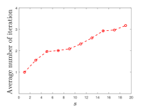
Figure 1: Average umber of iterations v.s. $s$ on data set $(m=500,n=1000,s=1:2:20,\nu=0.1,\sigma=0.05,p=1\%)$.

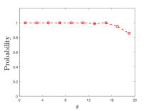
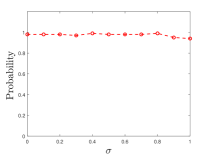
(a) $s$	(b) $\sigma$
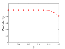
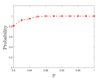
(c) $p$	(d) $p$

Figure 2: The exact support recovery probability v.s. $s$, $\sigma$ and $p$ on data set $(m=500,n=1000,s=1:2:20,\nu=0.1,\sigma=0.05,p=1\%)$ (panel (a)), $(m=500,n=1000,s=10,\nu=0.3,\sigma=0:0.1:1,p=5\%)$ (panel (b)) and $(m=500,n=1000,s=5,\nu=0.1,\sigma=0.05,p=0:2\%:20\%)$ (panel (c)), $(m=500,n=1000,s=5,\nu=0.1,\sigma=0.05,p=80\%:2\%:100\%)$ (panel (d)).

4.3 Support recovery

In this subsection we verify the support recovery property of GNA by studying how the exact support recovery probability depends on the sparsity level $s$, the noise level $\sigma$ and the of sign flips probability $p$. We test on date sets $(m=500,n=1000,s=1:2:20,\nu=0.1,\sigma=0.05,p=1\%)$, $(m=500,n=1000,s=10,\nu=0.3,\sigma=0:0.1:1,p=5\%)$, $(m=500,n=1000,s=5,\nu=0.1,\sigma=0.05,p=0:2\%:20\%)$, $(m=500,n=1000,s=5,\nu=0.1,\sigma=0.05,p=80\%:2\%:100\%)$ and show the corresponding results in panel (a)-(d) of Figure 2 respectively. As indicates by Figure 2, GNA recovers the underlying true support with high probability as long the sparsity level $s\leq\mathcal{O}(m/{\log n})$ even if the binary measurements is noisy and sign flipped. This confirms the theoretical investigations in Proposition 3.2.

4.4 Comparison with state-of-the-art

Now we compare our proposed model (6) and GNA Algorithm 1 with several state-of-the-art methods such as BIHT [22] (http://perso.uclouvain.be/laurent.jacques/index.php/Main/BIHTDemo), AOP [41] and PBAOP [21] (both AOP and PBAOP require to know the sign flips probability $p$, available at http://www.esat.kuleuven.be/stadius/ADB/huang/downloads/1bitCSLab.zip) and linear projection (LP) [40, 35], PDASC [20] (http://faculty.zuel.edu.cn/tjyjxxy/jyl/list.htm/). We use data set $(m=500,n=2500,s=5,\nu=0.2,\sigma=0.2,p=5\%)$, $(m=500,n=2500,s=5,\nu=0.3,\sigma=0.3,p=10\%)$, $(m=500,n=2500,s=5,\nu=0.5,\sigma=0.5,p=15\%)$, and $(m=1000,n=5000,s=10,\nu=0.2,\sigma=0.2,p=5\%)$, $(m=1000,n=5000,s=10,\nu=0.3,\sigma=0.3,p=10\%)$, $(m=1000,n=5000,s=10,\nu=0.5,\sigma=0.5,p=15\%)$. The average CPU time in seconds (Time (s)), the average of the $\ell_{2}$ error $\|\frac{\hat{x}}{\|\hat{x}\|}-\frac{x^{*}}{\|x^{*}\|}\|$ ($\ell_{2}$-Err) where $\hat{x}$ denotes the output of all the above mentioned methods, and the probability of exactly recovering true support (PrE ($\%$)) are reported in Table 1. As shown in Table 1, our GNA outperforms all the other state-of-the-art methods in terms of accuracy ($\ell_{2}$-Err and PrE $(\%)$) in all the settings. Meanwhile, GNA and LP archive the best performance on speed.

Table 1: Comparison GNA with state-of-the-art methods on CPU time in seconds (Time (s)), average $\ell_{2}$ error $\|\frac{\hat{x}}{\|\hat{x}\|}-\frac{x^{*}}{\|x^{*}\|}\|$ ($\ell_{2}$-Err), probability on exactly recovering of true support (PrE ($\%$)).

$(m=500,n=2500,s=5)$
(a) $(\nu=0.2,\sigma=0.2,p=5\%)$					(b) $(\nu=0.3,\sigma=0.3,p=10\%)$				(c) $(\nu=0.5,\sigma=0.5,p=15\%)$
Method	Time (s)	$\ell_{2}$-Err	PrE $(\%)$		Time (s)	$\ell_{2}$-Err	PrE $(\%)$		Time	$\ell_{2}$-Err	PrE
BIHT	3.39e-1	4.98e-1	33		3.72e-1	7.97e-1	1		3.39e-1	1.10e-0	0
AOP	9.18e-1	1.59e-1	98		9.86e-1	2.05e-1	92		9.28e-1	5.30e-1	30
LP	2.21e-2	4.22e-1	96		2.40e-2	4.36e-1	81		2.17e-2	5.43e-1	6
PBAOP	3.40e-1	1.56e-1	98		3.65e-1	2.06e-1	93		3.44e-1	5.56e-1	25
PDASC	9.49e-2	9.56e-2	98		9.10e-2	1.73e-1	86		7.05e-2	5.25e-1	24
GNA	1.53e-2	8.82e-2	100		1.73e-2	1.15e-1	99		1.48e-2	2.15e-1	82
$(m=1000,n=5000,s=10)$
(a) $(\nu=0.2,\sigma=0.2,p=5\%)$					(b) $(\nu=0.3,\sigma=0.3,p=10\%)$				(c) $(\nu=0.5,\sigma=0.5,p=15\%)$
Method	Time (s)	$\ell_{2}$-Err	PrE $(\%)$		Time (s)	$\ell_{2}$-Err	PrE $(\%)$		Time	$\ell_{2}$-Err	PrE
BIHT	1.35e-0	5.33e-1	10		1.32e-0	8.06e-1	0		1.29e-0	1.03e-0	0
AOP	3.77e-0	1.68e-1	98		3.69e-0	2.13e-1	88		3.52e-0	5.30e-1	7
LP	5.64e-2	4.41e-1	82		5.83e-2	4.46e-1	62		5.23e-2	5.88e-1	1
PBAOP	1.37e-0	1.59e-1	100		1.32e-0	2.12e-1	89		1.29e-0	5.81e-1	5
PDASC	3.64e-1	9.77e-2	98		3.05e-1	1.84e-1	79		2.52e-1	7.72e-1	4
GNA	6.02e-2	9.62e-2	100		5.93e-2	1.24e-1	99		5.94e-2	2.66e-1	59

Last, we compare our GNA with the aforementioned competitors to recover a one-dimensional signal and two-dimensional image from quantized measurements. The true signal and image are sparse under wavelet basis “Db1" [30]. Thus, the matrix $\Psi$ consist of random Gaussian matrix and an Harr wavelet transform with level $1$ and $2^{12}$, respectively. The target coefficients have $36$ and $1138$ nonzeros, and the size $\Psi$ are $2500\times 8000$ and $5000\times 128^{2}$. We set $\sigma=0.5$, $p=6\%$ and $\sigma=0.05$, $p=1\%$ and the measurements are quantized with bit depth $1$ and $6$ for the signal and image respectively. The recovered results are shown in Figure 3, Table 2 and Figure 4, Table 3 respectively. The decoding results by GNA are visually more appealing than others, as shown in Figure 3-4, which are further confirmed by the PSNR value reported in Table 2-3, defined as $\mathrm{PSNR}=10\cdot\log\frac{V^{2}}{\rm MSE}$, where $V$ is the maximum absolute value of the true signal/image, and MSE is the mean squared error of the reconstruction.

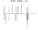
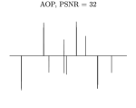
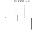
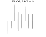
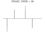
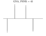
Figure 3: Reconstruction of the one-dimensional signal with $(m=2500,n=8000,s=36,\nu=0,\sigma=0.5,p=6\%)$.

Table 2: The CPU time in seconds and the PSNR of one-dimensional signal recovery with $(m=2500,n=8000,s=36,\nu=0,\sigma=0.5,p=6\%)$.

method	CPU time (s)	PSNR
BIHT	5.01	28
AOP	5.83	32
LP	0.12	32
PBAOP	5.65	31
PDASC	3.58	30
GNA	0.72	45

Table 3: The CPU time in seconds and the PSNR of two-dimensional image recovery with $(m=5000,n=128^{2},s=1138,\nu=0,\sigma=0.05,p=1\%)$.

method	CPU time (s)	PSNR
BIHT	40.7	17
AOP	20.0	17
LP	0.21	17
PBAOP	20.5	16
PDASC	21.2	19
GNA	5.73	23

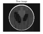
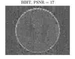
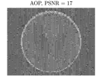
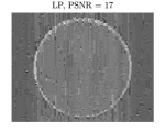
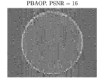
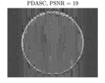
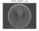
Figure 4: Reconstruction of the two-dimension image with $(m=5000,n=128^{2},s=1138,\nu=0,\sigma=0.05,p=1\%)$.

5 Conclusions

In this paper we consider decoding from binary measurements with noise and sign flips. We proposed the cardinality constraint least squares as a decoder. We prove that, up to a constant $c$, with high probability, the proposed decoder achieves a minimax estimation error as long as $m\geq\mathcal{O}(s\log n)$. Computationally, we utilize a generalized Newton algorithm (GNA) to solve the cardinality constraint minimization approximately with the cost of solving a small size least squares problem at each iteration. We prove that, with high probability, the $\ell_{\infty}$ norm of the estimation error between the output of GNA and the underlying target decay to $\mathcal{O}(\sqrt{\frac{\log n}{m}})$ with at most $\mathcal{O}(\log s)$ steps. Moreover, the underlying support can be recover with high probability in $\mathcal{O}(\log s)$ steps provide that the target signal is detectable. Extensive numerical experiments and comparison with other state-of-the-art 1-bit CS model demonstrates the robustness of our decoder and the efficiency of GNA algorithm.

Appendix A Preliminaries

Lemma A.1.

Let $\Psi\in\mathbb{R}^{m\times n}$ whose rows $\psi_{i}^{t}$ are independent subgaussian vectors in $\mathbb{R}^{n}$ with mean 0 and covariance matrix $\Sigma$. Let $m>n$. Then for every $t>0$ with probability at least $1-2\exp{(-C_{1}t^{2})}$, one has

$$(1-\tau)\sqrt{\gamma_{\mathrm{min}}(\Sigma)}\leq\sqrt{\gamma_{\textrm{min}}(\frac{\Psi^{t}\Psi}{m})}\leq\sqrt{\gamma_{\textrm{max}}(\frac{\Psi^{t}\Psi}{m})}\leq(1+\tau)\sqrt{\gamma_{\mathrm{max}}(\Sigma)},$$ (14)

and

$$\|\Psi^{t}\Psi/m-\Sigma\|\leq\max\{\tau,\tau^{2}\}\gamma_{\textrm{max}}(\Sigma),$$ (15)

where $\tau=C_{2}\sqrt{\frac{n}{m}}+\frac{t}{\sqrt{m}},$ and $C_{1},C_{2}$ are generic positive constants depending on the maximum subgaussian norm of rows of $\Psi$.

Proof.

Let $\Phi=\Psi\Sigma^{-\frac{1}{2}}$. Then the rows of $\Phi$ are independent sub-gaussian isotropic vectors. (14) follows from Theorem 5.39 and Lemma 5.36 of [39] and (15) is a direct consequence of Remark 5.40 of [39]. ∎

Lemma A.2.

Let $C_{3}\geq\|x^{*}\|_{1}$. If $m>\frac{4C_{1}}{C_{2}^{2}}\log n$, then with probability at least $1-2/n^{3}-2/n^{2}$, one has

$$\|\Psi^{t}(y-c\Psi x^{*})/m\|_{\infty}\leq\frac{2(1+|c|C_{3})}{\sqrt{C_{1}}}\sqrt{\frac{\log n}{m}}.$$ (16)

Proof.

See Lemma D.2 in [20]. ∎

Lemma A.3.

Define

$$C_{2s,\mathrm{min}}=\inf_{A\subset[n],|A|\leq 2s}\frac{\gamma_{\mathrm{min}}(\Psi_{A}^{t}\Psi_{A})}{m},$$

$$C_{2s,\mathrm{max}}=\sup_{A\subset[n],|A|\leq 2s}\frac{\gamma_{\mathrm{max}}(\Psi_{A}^{t}\Psi_{A})}{m}.$$

Then, with probability at least $1-4/n^{2}$,

$$C_{2s,\mathrm{min}}\geq\gamma_{\mathrm{min}}(\Sigma)/4,$$

$$C_{2s,\mathrm{max}}\leq 9\gamma_{\mathrm{max}}(\Sigma)/4,$$

as long as $m\geq\frac{16(C_{2}+1)^{2}}{C_{1}}s\log\frac{en}{s}$ and $s\leq\exp^{(1-\frac{C_{1}}{2})}n.$

Proof.

Given $A\subset[n],|A|\leq 2s$, we define the event

$$E_{A}=\{\sqrt{\frac{\gamma_{\mathrm{min}}(\Psi_{A}^{t}\Psi_{A})}{m}}>\sqrt{\gamma_{\mathrm{min}}(\Sigma)}(1-C_{2}\sqrt{\frac{2s}{m}}-\frac{t}{\sqrt{m}})\}.$$

Then,

$$\mathbb{P}[C_{2s,\mathrm{min}}>\gamma_{\mathrm{min}}(\Sigma)(1-C_{2} \sqrt{\frac{2s}{m}}-\frac{t}{\sqrt{m}})^{2}]=\mathbb{P}[\bigcap_{A\in[n],|A|\leq 2s}E_{A}]=\mathbb{P}[\bigcap_{A\in[n],|A|=\ell,1\leq\ell\leq 2s}E_{A}]$$

$$=1-\mathbb{P}[\bigcup_{A\in[n],|A|=\ell,1\leq\ell\leq 2s}\overline{E_{A}}]$$

$$\geq 1-\sum_{\ell=1}^{2s}\sum_{A\subset[n],|A|=\ell}(1-\mathbb{P}[E_{A}])$$

$$\geq 1-\sum_{\ell=1}^{2s}\sum_{A\subset[n],|A|\leq\ell}2\exp(-C_{1}t^{2})$$

$$=1-\sum_{\ell=1}^{2s}\binom{n}{\ell}2\exp(-C_{1}t^{2})$$

$$\geq 1-2(\frac{en}{2s})^{2s}\exp(-C_{1}t^{2}),$$

where the first inequality follows from the union bound, the second inequality follows from (14) by replacing $\Psi$ with $\Psi_{A}$, and the third inequality holds since

$$\sum_{\ell=1}^{2s}\binom{n}{\ell}\leq(\frac{n}{2s})^{2s}\sum_{\ell=0}^{2s}\binom{n}{\ell}(\frac{2s}{n})^{\ell}$$

$$\leq(\frac{n}{2s})^{2s}(1+\frac{2s}{n})^{n}$$

$$\leq(\frac{en}{2s})^{2s}.$$

Thus, by setting $t=\sqrt{\frac{4s}{C_{1}}\log\frac{en}{s}}$, we derive with probability at least $1-2/(\frac{en}{s})^{2s}\geq 1-2/n^{2}$

$$C_{2s,\mathrm{min}} >\gamma_{\mathrm{min}}(\Sigma)(1-C_{2}\sqrt{\frac{2s}{m}}-\frac{t}{\sqrt{m}})^{2}$$

$$\geq\gamma_{\mathrm{min}}(\Sigma)(1-(C_{2}+1)\sqrt{\frac{4s}{mC_{1}}\log\frac{en}{s}})^{2}$$

$$\geq\gamma_{\mathrm{min}}(\Sigma)/4,$$

where the second inequality follows from the assumption $s\leq\exp^{(1-\frac{C_{1}}{2})}n$ and , i.e.,

$$\sqrt{\frac{2s}{m}}\leq\sqrt{\frac{4s}{mC_{1}}\log\frac{en}{s}}<1,$$

and the last inequality follows from the assumption $m\geq\frac{16(C_{2}+1)^{2}}{C_{1}}s\log\frac{en}{s}$. Define event

$$\widetilde{E}_{A}=\{\sqrt{\frac{\gamma_{\mathrm{max}}(\Psi_{A}^{t}\Psi_{A})}{m}}>\sqrt{\gamma_{\mathrm{max}}(\Sigma)}(1+C_{2}\sqrt{\frac{2s}{m}}+\frac{t}{\sqrt{m}})\}.$$

Then,

$$\mathbb{P}[C_{2s,\mathrm{max}}>\gamma_{max}(\Sigma)(1+C_{2}\sqrt{\frac{2s}{m}}+\frac{t}{\sqrt{m}})^{2}] =\mathbb{P}[\bigcup_{A\subset[n],|A|\leq 2s}\widetilde{E}_{A}]$$

$$=\mathbb{P}[\bigcup_{A\subset[n],|A|=\ell,1\leq\ell\leq 2s}\widetilde{E}_{A}]$$

$$\leq\sum_{\ell=1}^{2s}\sum_{A\in[n],|A|\leq\ell}2\exp(-C_{1}t^{2})$$

$$\leq(\sum_{\ell=1}^{2s}\binom{n}{\ell})2\exp(-C_{1}t^{2})$$

$$\leq 2(\frac{en}{s})^{2s}\exp(-C_{1}t^{2}),$$

which implies with probability at least $1-2(\frac{en}{s})^{2s}\exp(-C_{1}t^{2})$,

$$C_{2s,\mathrm{max}}\leq\gamma_{max}(\Sigma)(1+C_{2}\sqrt{\frac{2s}{m}}+\frac{t}{\sqrt{m}})^{2}.$$

We finish the proof by setting $t=\sqrt{\frac{4s}{C_{1}}\log\frac{en}{s}}$ and some algebra. ∎

Appendix B Proof of Theorem 2.1

Proof.

Let

$$\tilde{x}^{*} =cx^{*},$$ (17)

$$R =y-\Psi\tilde{x}^{*},$$ (18)

and $\Delta=x_{\ell_{0}}-\tilde{x}^{*}$, $\mathcal{A}=\mathrm{supp}(R)$. By the definition $x_{\ell_{0}}$, we have $\|x_{\ell_{0}}\|_{0}\leq s,$ $|\mathcal{A}|\leq 2s$ and

$$\frac{1}{2m}\|y-\Psi x_{\ell_{0}}\|_{2}^{2}\leq\frac{1}{2m}\|y-\Psi\tilde{x}^{*}\|_{2}^{2}.$$ (19)

Then,

$$\gamma_{\mathrm{min}}(\Sigma)\|\Delta\|_{2}^{2}/4 \leq C_{2s,\mathrm{min}}\|\Delta\|_{2}^{2}\leq\frac{1}{2m}\|\Psi\Delta\|_{2}^{2}$$

$$\leq\langle\Delta,\Psi^{t}R/m\rangle\leq\|\Delta\|_{2}\|\Psi_{\mathcal{A}}^{t}R/m\|_{2}$$

$$\leq\sqrt{2s}\|\Delta\|_{2}\|\Psi^{t}R/m\|_{\infty}$$

$$\leq\|\Delta\|_{2}\frac{2(1+|c|C_{3})}{\sqrt{C_{1}}}\sqrt{\frac{2s\log n}{m}},$$

where, the first inequality holds with probability at least $1-2/n^{2}$ by Lemma A.3, and the second inequality uses the definition of $C_{2s,\mathrm{min}}$, and the third inequality dues to (19) and some algebra, and the third on uses Cauchy Schwartz inequality, and the fourth inequity follow from $|\mathcal{A}|\leq 2s$ and Cauchy Schwartz inequality, and the last inequality holds with probability at least $1-2/n^{3}-2/n^{2}$ by Lemma A.2. The above display implies, with probability at least $1-2/n^{3}-4/n^{2}$

$$\|x_{\ell_{0}}/c-x^{*}\|\leq\frac{12(1/|c|+C_{3})}{\sqrt{C_{1}}\gamma_{\mathrm{min}}(\Sigma)}\sqrt{\frac{s\log n}{m}}.$$

We finish the proof by substituting $c$ and some algebra. ∎

Appendix C Proof of Lemma 3.1

Proof.

Flowing Theorem 2.2 in [5], we just need to show that $\Psi$ is $s$-regular i.e., $\frac{\gamma_{\mathrm{min}}(\Psi_{A}^{t}\Psi_{A})}{m}>0$ with $A\subset[n],|A|\leq s$, and to calculate the Lipschitz constant of the gradient of the least squares loss in (1) restricted on $s$ sparse vectors, i.e., $\frac{\gamma_{\mathrm{max}}(\Psi_{A}^{t}\Psi_{A})}{m}$ with $A\subset[n],|A|\leq 2s$. By Lemma A.3 with probability at least $1-4/n^{2}$, $\Psi$ is $s$-regular and the Lipschitz constant is bounded by $9\gamma_{\mathrm{max}}(\Sigma)/4$. ∎

Appendix D Proof of Proposition 3.1

Proof.

Denote $D^{k}=-(H^{k})^{-1}F(w^{k})$. Then,

$$w^{k+1}=w^{k}-(H^{k})^{-1}F(w^{k}),$$

can be recast as

$$H^{k}D^{k} =-F(w^{k})$$ (20)

$$w^{k+1} =w^{k}+D^{k}.$$ (21)

Partition $w^{k}$, $D^{k}$ and $F(w^{k})$ according to $A^{k}$ and ${I}^{k}$ such that

$$w^{k}=\left(\begin{array}[]{c}x_{A^{k}}^{k}\\ x_{I^{k}}^{k}\\ d_{{A}^{k}}^{k}\\ d_{{I}^{k}}^{k}\\ \end{array}\right),\ \ D^{k}=\left(\begin{array}[]{c}D^{x}_{A^{k}}\\ D^{x}_{I^{k}}\\ D^{d}_{A^{k}}\\ D^{d}_{{I}^{k}}\\ \end{array}\right),$$ (22)

$$F(w^{k})=\left[\begin{array}[]{c}-d_{{A}^{k}}^{k}\\ x_{{I}^{k}}^{k}\\ \Psi^{t}_{{A}^{k}}\Psi_{{A}^{k}}x_{{A}^{k}}^{k}+\Psi^{t}_{{A}^{k}}\Psi_{{I}^{k}}x_{{I}^{k}}^{k}+md_{{A}^{k}}^{k}-\Psi^{t}_{{A}^{k}}y\\ \Psi^{t}_{{I}^{k}}\Psi_{\mathcal{A}^{k}}x_{\mathcal{A}^{k}}^{k}+\Psi^{t}_{{I}^{k}}\Psi_{{I}^{k}}x_{{I}^{k}}^{k}+md_{{I}^{k}}^{k}-\Psi^{t}_{{I}^{k}}y\end{array}\right].$$ (23)

Substituting (22)-(23) and $H^{k}$ into (20), we have

$$(d_{{A}^{k}}^{k}+D^{d}_{\mathcal{A}_{k}}) =\mathbf{0}_{A^{k}},$$ (24)

$$x^{k}_{{I}^{k}}+D^{x}_{{I}^{k}} =\textbf{0}_{I^{k}},$$ (25)

$$\Psi^{t}_{{A}^{k}}\Psi_{{A}^{k}}(x_{{A}^{k}}^{k}+D^{x}_{{A}^{k}}) =\Psi^{t}_{{A}^{k}}y-m(d_{{A}^{k}}^{k}+D^{d}_{{A}^{k}})-\Psi^{t}_{{A}^{k}}\Psi_{{I}^{k}}(x^{k}_{{I}^{k}}+D^{x}_{{I}^{k}}),$$ (26)

$$m(d_{{I}^{k}}^{k}+D^{d}_{{I}^{k}}) =\Psi^{t}_{{I}^{k}}y-\Psi^{t}_{{I}^{k}}\Psi_{{A}^{k}}(x_{{A}^{k}}^{k}+D^{x}_{{A}^{k}})-\Psi^{t}_{{A}^{k}}\Psi_{{I}^{k}}(x_{{I}^{k}}^{k}+D^{x}_{{I}^{k}}).$$ (27)

It follows from (21) that

$$\left(\begin{array}[]{c}x_{{A}^{k}}^{k+1}\\ x_{{I}^{k}}^{k+1}\\ d_{{A}^{k}}^{k+1}\\ d_{{I}^{k}}^{k+1}\\ \end{array}\right)=\left(\begin{array}[]{c}x_{{I}^{k}}^{k}+D^{x}_{{I}^{k}}\\ d_{{A}^{k}}^{k}+D^{d}_{{A}^{k}}\\ x_{{A}^{k}}^{k}+D^{x}_{{A}^{k}}\\ d_{{I}^{k}}^{k}+D^{d}_{{I}^{k}}\\ \end{array}\right).$$ (28)

Substituting (28) into (24) - (27), we get (11) of Algorithm 1. This completes the proof. ∎

Appendix E Proof of Theorem 3.1

Let $A^{*}=\mathrm{supp}(x^{*})$ and $F(x)=\|y-\Psi x\|^{2}_{2}/m$ be the least squares loss in (6). And recall $\tilde{x}^{*}=cx^{*}$ in (17) and $R=y-\Psi\tilde{x}^{*}$ in (18). By (11), it is easy to see that

$$d^{k}=-\nabla F(x^{k}),\ \ \langle d^{k},x^{k}\rangle=0,\ \ k\geq 1.$$

The proof of Theorem 3.1 is based on the following Lemmas E.1-E.3, whose proof are shown in Appendix F.

Lemma E.1.

Let $\mathcal{A}^{k}=A^{k}\backslash A^{k-1}$ and $\varrho_{k}=\frac{|\mathcal{A}^{k}|}{|\mathcal{A}^{k}|+|A^{*}\backslash A^{k-1}|}$, $k\geq 1.$

$$2C_{*}\varrho_{k}(F(x^{k})-F(\tilde{x}^{*}))\leq\|d^{k}_{\mathcal{A}^{k}}\|_{1}\|d^{k}_{\mathcal{A}^{k}}\|_{\infty}.$$

Lemma E.2.

Let $\zeta=1-\frac{2\eta C_{*}(1-\eta\sqrt{s}C^{*})}{\sqrt{s}(1+s)}\in(0,1).$ It holds

$$F(x^{k+1})-F(\tilde{x}^{*})\leq\zeta(F(x^{k})-F(\tilde{x}^{*})),$$

before Algorithm GNA terminates.

Lemma E.3.

Let $\eta\in(0,\frac{1}{C^{*}\sqrt{s}})$ and $x^{0}=\mathbf{0}$ in GNA. Then we have

$$\|x^{k}/c-x^{*}\|_{\infty}\leq\zeta^{k/2}(\sqrt{\frac{2\|\Psi^{t}R/m\|_{\infty}\|x^{*}\|_{1}}{C_{*}|c|}}+\|x^{*}\|_{1}\sqrt{\frac{C^{*}}{C_{*}}})+\frac{2\|\Psi^{t}R/m\|_{\infty}}{C_{*}|c|}.$$ (29)

Proof.

By definition $C^{*}\leq C_{2s,\mathrm{max}}$. Then by Lemma A.3, the step size $\eta\in(0,\frac{4}{9\gamma_{\mathrm{max}}(\Sigma)\sqrt{s}})$ satisfying Lemma E.3 with probability at least $1-4/n^{2}$. By the assumption $\|x^{*}\|_{\Sigma}=1$ and Cauchy Schwartz inequality, we get

$$\|x^{*}\|_{1}\leq\sqrt{\frac{s}{\gamma_{\mathrm{min}}(\Sigma)}}.$$ (30)

By Lemma A.2,

$$\|\Psi^{t}R/m\|_{\infty}\leq\frac{2(1+|c|C_{3})}{\sqrt{C_{1}}}\sqrt{\frac{\log n}{m}}$$ (31)

holds with probability at least $1-2/n^{3}-2/n^{2}$. Substituting (30) and (31) into (29) and some algebra completes the proof. ∎

Appendix F Proof of Lemmas E.1-E.3

F.1 Proof of Lemma E.1

Proof.

In the scenario $A^{k}=A^{k-1}$ or $F(x^{k})\leq F(\tilde{x}^{*})$, the desired result holds trivially. Therefore, we assume $A^{k}\neq A^{k-1}$ and $F(x^{k})>F(\tilde{x}^{*})$. By the definition of $C_{*},C^{*}$ in (12) and Taylor expansion we have,

$$\frac{C_{*}}{2}\|\tilde{x}^{*}-x^{k}\|_{1}\|\tilde{x}^{*}-x^{k}\|_{\infty}\leq F(\tilde{x}^{*})-F(x^{k})+\langle d^{k},{\tilde{x}^{*}-x^{k}}\rangle$$

The above display implies,

$$\langle d^{k},\tilde{x}^{*}\rangle=\langle d^{k},{\tilde{x}^{*}-x^{k}}\rangle$$

$$\geq\frac{C_{*}}{2}\|\tilde{x}^{*}-x^{k}\|_{1}\|\tilde{x}^{*}-x^{k}\|_{\infty}+F(x^{k})-F(\tilde{x}^{*})$$

$$\geq\sqrt{2C_{*}}\sqrt{\|\tilde{x}^{*}-x^{k}\|_{1}\|\tilde{x}^{*}-x^{k}\|_{\infty}}\sqrt{F(x^{k})-F(\tilde{x}^{*})}.$$

By the definition of $A^{k}$ in (10) and $x^{k},d^{k}$ in (11), $\mathcal{A}^{k}$ contains the first $|\mathcal{A}^{k}|$-largest elements in absolute value of $d^{k}$ and $\mathrm{supp}(d^{k})\bigcap\mathrm{supp}(\tilde{x}^{*})=A^{*}\backslash A^{k-1}.$ By the definition of $\varrho_{k}$ and Cauchy Schwartz inequality, we have

$$\langle d^{k},\tilde{x}^{*}\rangle\leq\frac{1}{\sqrt{\varrho_{k}}}\|d^{k}_{\mathcal{A}^{k}}\|_{2}\|\tilde{x}_{A^{*}\backslash A^{k-1}}^{*}\|_{2}$$

$$=\frac{1}{\sqrt{\varrho_{k}}}\|d^{k}_{\mathcal{A}^{k}}\|_{2}\|(\tilde{x}^{*}-x^{k})_{A^{*}\backslash A^{k-1}}\|_{2}$$

$$\leq\frac{1}{\sqrt{\varrho_{k}}}\sqrt{\|d^{k}_{\mathcal{A}^{k}}\|_{1}\|d^{k}_{\mathcal{A}^{k}}\|_{\infty}}\sqrt{\|\tilde{x}^{*}-x^{k}\|_{1}\|\tilde{x}^{*}-x^{k}\|_{\infty}}.$$

We finish the proof by combing the above two displays. ∎

F.2 Proof of Lemma E.2

Proof.

Let $u^{k}=x^{k}+\eta d^{k},\ \ k\geq 1$. By the definition of $u^{k}$ and $A^{k}$ in (10) and $x^{k},d^{k}$ in (11), we have

$$\langle-d^{k+1},u^{k+1}|_{A^{k+1}}-x^{k+1}\rangle=\langle-d^{k+1},u^{k+1}|_{A^{k+1}}\rangle=\langle-d^{k+1}_{A^{k+1}\backslash A^{k}},u^{k+1}_{A^{k+1}\backslash A^{k}}\rangle,$$

$$|A^{k}\backslash A^{k+1}|=|A^{k+1}\backslash A^{k}|,\ \ u_{A^{k}\backslash A^{k+1}}^{k+1}=x_{A^{k}\backslash A^{k+1}}^{k+1},\ \ u_{A^{k+1}\backslash A^{k}}^{k+1}=\eta d^{k+1}_{A^{k+1}\backslash A^{k}},$$

$$\|u_{A^{k}\backslash A^{k+1}}^{k+1}\|_{1}=\|x_{A^{k}\backslash A^{k+1}}^{k+1}\|_{1}\leq\|u_{A^{k+1}\backslash A^{k}}^{k+1}\|_{1},\ \ \max\{\|u_{A^{k+1}\backslash A^{k}}^{k+1}\|_{\infty},\|x_{A^{k}\backslash A^{k+1}}^{k+1}\|_{\infty}\}=\|u_{A^{k+1}\backslash A^{k}}^{k+1}\|_{\infty}.$$

Then,

$$\|u^{k+1}|_{A^{k+1}}-x^{k+1}\|_{1}=\|u^{k+1}|_{A^{k+1}\backslash A^{k}}+u^{k+1}|_{A^{k+1}\bigcap A^{k}}-x^{k+1}|_{A^{k+1}\bigcap A^{k}}-x^{k+1}|_{A^{k}\backslash A^{k+1}}\|_{1}$$

$$=\|u_{A^{k+1}\backslash A^{k}}^{k+1}\|_{1}+\|u_{A^{k+1}\bigcap A^{k}}^{k+1}-x_{A^{k+1}\bigcap A^{k}}^{k+1}\|_{1}+\|x_{A^{k}\backslash A^{k+1}}^{k+1}\|_{1}$$

$$=\|u_{A^{k+1}\backslash A^{k}}^{k+1}\|_{1}+\|x_{A^{k}\backslash A^{k+1}}^{k+1}\|_{1}\leq 2\|u_{A^{k+1}\backslash A^{k}}^{k+1}\|_{1}=2\eta\|d_{A^{k+1}\backslash A^{k}}^{k+1}\|_{1},$$ (32)

$$\|u^{k+1}|_{A^{k+1}}-x^{k+1}\|_{\infty}=\|u_{A^{k+1}\backslash A^{k}}^{k+1}\|_{\infty}+\|x_{A^{k}\backslash A^{k+1}}^{k+1}\|_{\infty}$$

$$=\max\{\|u_{A^{k+1}\backslash A^{k}}^{k+1}\|_{\infty},\|x_{A^{k}\backslash A^{k+1}}^{k+1}\|_{\infty}\}=\|u_{A^{k+1}\backslash A^{k}}^{k+1}\|_{\infty}=\eta\|d_{A^{k+1}\backslash A^{k}}^{k+1}\|_{\infty}.$$ (33)

By (F.2)-(F.2) and the definition of $C^{*}$ in (12) and Taylor expansion, we get

$$F(u^{k+1}|_{A^{k+1}})-F(x^{k+1})$$

$$\leq\langle-d^{k+1},u^{k+1}|_{A^{k+1}}-x^{k+1}\rangle+\frac{C^{*}}{2}\|u^{k+1}|_{A^{k+1}}-x^{k+1}\|_{1}\|u^{k+1}|_{A^{k+1}}-x^{k+1}\|_{\infty}$$

$$\leq\langle-d^{k+1}_{A^{k+1}\backslash A^{k}},u^{k+1}_{A^{k+1}\backslash A^{k}}\rangle+\frac{C^{*}}{2}2\eta\|d_{A^{k+1}\backslash A^{k}}^{k+1}\|_{1}\eta\|d_{A^{k+1}\backslash A^{k}}^{k+1}\|_{\infty}$$

$$\leq-\eta\|d_{A^{k+1}\backslash A^{k}}^{k+1}\|_{2}^{2}+\eta^{2}C^{*}\|d_{A^{k+1}\backslash A^{k}}^{k+1}\|_{1}\|d_{A^{k+1}\backslash A^{k}}^{k+1}\|_{\infty}$$

$$\leq(-\frac{\eta}{\sqrt{s}}+\eta^{2}C^{*})\|d_{A^{k+1}\backslash A^{k}}^{k+1}\|_{1}\|d_{A^{k+1}\backslash A^{k}}^{k+1}\|_{\infty}.$$

Then the by the definition of $x^{k+1}$ and the above display, we deduce,

$$F(x^{k+1})-F(\tilde{x}^{*})-(F(x^{k})-F(\tilde{x}^{*}))\leq F(u^{k}|_{A^{k}})-F(x^{k})$$

$$\leq(-\frac{\eta}{\sqrt{s}}+\eta^{2}C^{*})\|d_{A^{k}\backslash A^{k-1}}^{k}\|_{1}\|d_{A^{k}\backslash A^{k-1}}^{k}\|_{\infty}$$

$$\leq(-\frac{\eta}{\sqrt{s}}+\eta^{2}C^{*})2C_{*}\varrho_{k}(F(x^{k})-F(\tilde{x}^{*}))$$

$$\leq(-\frac{\eta}{\sqrt{s}}+\eta^{2}C^{*})2C_{*}\frac{1}{1+s}(F(x^{k})-F(\tilde{x}^{*}))$$

where the third inequality uses $\eta<\frac{1}{\sqrt{s}C^{*}}$ and Lemma E.1 and the fourth inequality holds due to $\varrho_{k}\geq\frac{1}{s+1}$. We finish the proof by rearranging term in the above display. ∎

Appendix G Proof of Lemma E.3

Proof.

If $\|x^{k}-\tilde{x}^{*}\|_{\infty}<\frac{2\|\Psi^{t}R/m\|_{\infty}}{C_{*}}$, Lemma E.3 holds trivially. Therefore, we consider the case

$$\|x^{k}-\tilde{x}^{*}\|_{\infty}\geq\frac{2\|\Psi^{t}R/m\|_{\infty}}{C_{*}}.$$

It follows from the the definition of $C_{*}$ and Taylor expansion that

$$F(x^{k})-F(\tilde{x}^{*})\geq\langle\nabla F(\tilde{x}^{*}),x^{k}-\tilde{x}^{*}\rangle+\frac{C_{*}}{2}\|x^{k}-\tilde{x}^{*}\|_{1}\|x^{k}-\tilde{x}^{*}\|_{\infty}$$

$$\geq-\|\Psi^{t}R/m\|_{\infty}\|x^{k}-\tilde{x}^{*}\|_{1}+\frac{C_{*}}{2}\|x^{k}-\tilde{x}^{*}\|_{1}\|x^{k}-\tilde{x}^{*}\|_{\infty}.$$

The above display and the fact

$$(\|x^{k}-\tilde{x}^{*}\|_{1}-\|x^{k}-\tilde{x}^{*}\|_{\infty})(\frac{C_{*}}{2}\|x^{k}-\tilde{x}^{*}\|_{\infty}-\|\Psi^{t}R/m\|_{\infty})\geq 0,$$

imply $g(\|x^{k}-\tilde{x}^{*}\|_{\infty})\leq 0$, where the univariate quadratic function

$$g(t)=\frac{C_{*}}{2}t^{2}-\|\Psi^{t}R/m\|_{\infty}t-(F(x^{k})-F(\tilde{x}^{*})).$$

Therefore, we have

$$\|x^{k}-\tilde{x}^{*}\|_{\infty} \leq\frac{\|\Psi^{t}R/m\|_{\infty}+\sqrt{\|\Psi^{t}R/m\|_{\infty}^{2}+2C_{*}(F(x^{k})-F(\tilde{x}^{*}))}}{C_{*}}$$

$$\leq\sqrt{\frac{2\max\{F(x^{k})-F(\tilde{x}^{*}),0\}}{C_{*}}}+\frac{2\|\Psi^{t}R/m\|_{\infty}}{C_{*}}.$$ (34)

On the other hand,

$$F(x^{k})-F(\tilde{x}^{*})\|_{\infty}\leq\zeta^{k}(F(x^{0})-F(\tilde{x}^{*}))$$

$$\leq\zeta^{k}(\langle-\Psi^{t}R/m,x^{0}-\tilde{x}^{*}\rangle+\frac{C^{*}}{2}\|x^{0}-\tilde{x}^{*}\|_{1}\|x^{0}-\tilde{x}^{*}\|_{\infty})$$

$$\leq\zeta^{k}(\|\Psi^{t}R/m\|_{\infty}\|x^{0}-\tilde{x}^{*}\|_{1}+\frac{C^{*}}{2}\|x^{0}-\tilde{x}^{*}\|_{1}\|x^{0}-\tilde{x}^{*}\|_{\infty})$$

$$\leq\zeta^{k}(\|\Psi^{t}R/m\|_{\infty}|c|\|x^{*}\|_{1}+\frac{C^{*}}{2}c^{2}\|x^{*}\|_{1}^{2})$$ (35)

where the first inequality uses Lemma E.2 and the second inequality uses the definition of $C^{*}$ in (12) and Taylor expansion, the third inequality follows from Cauchy Schwartz inequality, and the last one uses $x^{0}=\mathbf{0}$. Combing the (G) and (G) we get

$$\|x^{k}-\tilde{x}^{*}\|_{\infty} \leq\zeta^{k/2}\sqrt{(2\|\Psi^{t}R/m\|_{\infty}|c|\|x^{*}\|_{1}/C_{*}+\frac{C^{*}}{C_{*}}c^{2}\|x^{*}\|_{1}^{2})}+\frac{2\|\Psi^{t}R/m\|_{\infty}}{C_{*}}$$

$$\leq\zeta^{k/2}(\sqrt{2\|\Psi^{t}R/m\|_{\infty}|c|\|x^{*}\|_{1}/C_{*}}+|c|\|x^{*}\|_{1}\sqrt{\frac{C^{*}}{C_{*}})})+\frac{2\|\Psi^{t}R/m\|_{\infty}}{C_{*}}.$$

We completes the proof by diving $|c|$. ∎

Appendix H Proof of Proposition 3.2

Proof.

By (13) in Theorem 3.1 and the assumption on $|x^{*}|_{\mathrm{min}}$, we get $\mathrm{supp}(x^{*})\subseteq A^{k}$. Hence, $\mathrm{supp}(x^{*})=\subseteq A^{k}$ since we assume $\mathrm{supp}(x^{*})=s$. Then $\mathrm{supp}(x^{*})=A^{k}=A^{k+1}$ as long as $k\geq\log_{1/\zeta}(\frac{sm}{\log n}\frac{C^{*}C_{1}|c|^{2}}{16C_{*}(1+|c|C_{3})^{2}\gamma_{\mathrm{min}}(\Sigma)}).$ This completes the proof. ∎

References

• [1] M. E. Ahsen and M. Vidyasagar. An approach to one-bit compressed sensing based on probably approximately correct learning theory. The Journal of Machine Learning Research, 20(1):408–430, 2019.
• [2] A. Ai, A. Lapanowski, Y. Plan, and R. Vershynin. One-bit compressed sensing with non-gaussian measurements. Linear Algebra and its Applications, 441:222–239, 2014.
• [3] R. Baraniuk, S. Foucart, D. Needell, Y. Plan, and M. Wootters. One-bit compressive sensing of dictionary-sparse signals. arXiv preprint arXiv:1606.07531, 2016.
• [4] R. G. Baraniuk, S. Foucart, D. Needell, Y. Plan, and M. Wootters. Exponential decay of reconstruction error from binary measurements of sparse signals. IEEE Transactions on Information Theory, 63(6):3368–3385, 2017.
• [5] A. Beck and Y. C. Eldar. Sparsity constrained nonlinear optimization: Optimality conditions and algorithms. SIAM Journal on Optimization, 23(3):1480–1509, 2013.
• [6] P. T. Boufounos. Greedy sparse signal reconstruction from sign measurements. In Signals, Systems and Computers, 2009 Conference Record of the Forty-Third Asilomar Conference on, pages 1305–1309. IEEE, 2009.
• [7] P. T. Boufounos and R. G. Baraniuk. 1-bit compressive sensing. In Information Sciences and Systems, 2008. CISS 2008. 42nd Annual Conference on, pages 16–21. IEEE, 2008.
• [8] D. R. Brillinger. A generalized linear model with gaussian regressor variables. A Festschrift For Erich L. Lehmann, page 97, 1982.
• [9] E. J. Candés, J. Romberg, and T. Tao. Robust uncertainty principles: Exact signal reconstruction from highly incomplete frequency information. IEEE Trans. Inform. Theory, 52(2):489–509, 2006.
• [10] D.-Q. Dai, L. Shen, Y. Xu, and N. Zhang. Noisy 1-bit compressive sensing: models and algorithms. Applied and Computational Harmonic Analysis, 40(1):1–32, 2016.
• [11] D. L. Donoho. Compressed sensing. IEEE Trans. Inform. Theory, 52(4):1289–1306, 2006.
• [12] M. Fazel, E. Candes, B. Recht, and P. Parrilo. Compressed sensing and robust recovery of low rank matrices. In Signals, Systems and Computers, 2008 42nd Asilomar Conference on, pages 1043–1047. IEEE, 2008.
• [13] S. Foucart. Hard thresholding pursuit: an algorithm for compressive sensing. SIAM J. Numer. Anal., 49(6):2543–2563, 2011.
• [14] S. Foucart and H. Rauhut. A mathematical introduction to compressive sensing, volume 1. Birkhäuser Basel, 2013.
• [15] L. Goldstein, S. Minsker, and X. Wei. Structured signal recovery from non-linear and heavy-tailed measurements. IEEE Transactions on Information Theory, 64(8):5513–5530, 2018.
• [16] S. Gopi, P. Netrapalli, P. Jain, and A. Nori. One-bit compressed sensing: Provable support and vector recovery. In International Conference on Machine Learning, pages 154–162, 2013.
• [17] A. Gupta, R. Nowak, and B. Recht. Sample complexity for 1-bit compressed sensing and sparse classification. In Information Theory Proceedings (ISIT), 2010 IEEE International Symposium on, pages 1553–1557. IEEE, 2010.
• [18] J. Haupt and R. Baraniuk. Robust support recovery using sparse compressive sensing matrices. In Information Sciences and Systems (CISS), 2011 45th Annual Conference on, pages 1–6. IEEE, 2011.
• [19] J. Huang, Y. Jiao, Y. Liu, and X. Lu. A constructive approach to l 0 penalized regression. The Journal of Machine Learning Research, 19(1):403–439, 2018.
• [20] J. Huang, Y. Jiao, X. Lu, and L. Zhu. Robust decoding from 1-bit compressive sampling with ordinary and regularized least squares. SIAM Journal on Scientific Computing, 40(4):A2062–A2086, 2018.
• [21] X. Huang, L. Shi, M. Yan, and J. A. Suykens. Pinball loss minimization for one-bit compressive sensing. arXiv preprint arXiv:1505.03898, 2015.
• [22] L. Jacques, K. Degraux, and C. De Vleeschouwer. Quantized iterative hard thresholding: Bridging 1-bit and high-resolution quantized compressed sensing. arXiv preprint arXiv:1305.1786, 2013.
• [23] L. Jacques, J. N. Laska, P. T. Boufounos, and R. G. Baraniuk. Robust 1-bit compressive sensing via binary stable embeddings of sparse vectors. IEEE Transactions on Information Theory, 59(4):2082–2102, 2013.
• [24] Y. Jiao, B. Jin, and X. Lu. A primal dual active set with continuation algorithm for the l0-regularized optimization problem. Applied and Computational Harmonic Analysis, 39(3):400–426, 2015.
• [25] K. Knudson, R. Saab, and R. Ward. One-bit compressive sensing with norm estimation. IEEE Transactions on Information Theory, 62(5):2748–2758, 2016.
• [26] J. N. Laska and R. G. Baraniuk. Regime change: Bit-depth versus measurement-rate in compressive sensing. IEEE Transactions on Signal Processing, 60(7):3496–3505, 2012.
• [27] J. N. Laska, Z. Wen, W. Yin, and R. G. Baraniuk. Trust, but verify: Fast and accurate signal recovery from 1-bit compressive measurements. IEEE Transactions on Signal Processing, 59(11):5289–5301, 2011.
• [28] K.-C. Li and N. Duan. Regression analysis under link violation. The Annals of Statistics, pages 1009–1052, 1989.
• [29] W. Liu, D. Gong, and Z. Xu. One-bit compressed sensing by greedy algorithms. Numerical Mathematics: Theory, Methods and Applications, 9(2):169–184, 2016.
• [30] S. Mallat. A wavelet tour of signal processing: the sparse way. Academic press, 2008.
• [31] M. Neykov, J. S. Liu, and T. Cai. L1-regularized least squares for support recovery of high dimensional single index models with gaussian designs. The Journal of Machine Learning Research, 17(1):2976–3012, 2016.
• [32] Y. Plan and R. Vershynin. One-bit compressed sensing by linear programming. Communications on Pure and Applied Mathematics, 66(8):1275–1297, 2013.
• [33] Y. Plan and R. Vershynin. Robust 1-bit compressed sensing and sparse logistic regression: A convex programming approach. IEEE Transactions on Information Theory, 59(1):482–494, 2013.
• [34] Y. Plan and R. Vershynin. The generalized lasso with non-linear observations. IEEE Transactions on information theory, 62(3):1528–1537, 2016.
• [35] Y. Plan, R. Vershynin, and E. Yudovina. High-dimensional estimation with geometric constraints. Information and Inference: A Journal of the IMA, 6(1):1–40, 2017.
• [36] G. Raskutti, M. J. Wainwright, and B. Yu. Minimax rates of estimation for high-dimensional linear regression over lq-balls. IEEE transactions on information theory, 57(10):6976–6994, 2011.
• [37] K. Sayood. Introduction to data compression. Morgan Kaufmann, 2017.
• [38] J. Shen and P. Li. On the iteration complexity of support recovery via hard thresholding pursuit. In Proceedings of the 34th International Conference on Machine Learning-Volume 70, pages 3115–3124. JMLR, 2017.
• [39] R. Vershynin. Introduction to the non-asymptotic analysis of random matrices. arXiv preprint arXiv:1011.3027, 2010.
• [40] R. Vershynin. Estimation in high dimensions: a geometric perspective. In Sampling theory, a renaissance, pages 3–66. Springer, 2015.
• [41] M. Yan, Y. Yang, and S. Osher. Robust 1-bit compressive sensing using adaptive outlier pursuit. IEEE Transactions on Signal Processing, 60(7):3868–3875, 2012.
• [42] X.-T. Yuan, P. Li, and T. Zhang. Gradient hard thresholding pursuit. Journal of Machine Learning Research, 18:166–1, 2017.
• [43] C.-H. Zhang and T. Zhang. A general theory of concave regularization for high-dimensional sparse estimation problems. Statist. Sci., 27(4):576–593, 2012.
• [44] L. Zhang, J. Yi, and R. Jin. Efficient algorithms for robust one-bit compressive sensing. In International Conference on Machine Learning, pages 820–828, 2014.
• [45] Y. Zhang, M. J. Wainwright, M. I. Jordan, et al. Optimal prediction for sparse linear models? lower bounds for coordinate-separable m-estimators. Electronic Journal of Statistics, 11(1):752–799, 2017.
• [46] A. Zymnis, S. Boyd, and E. Candes. Compressed sensing with quantized measurements. IEEE Signal Processing Letters, 17(2):149–152, 2010.