ToGCom: An Asymmetric Sybil Defense

Abstract

Proof-of-work (PoW) is one of the most common techniques to defend against Sybil attacks. Unfortunately, current PoW defenses have two main drawbacks. First, they require work to be done even in the absence of attack. Second, during an attack, they require the good identities (IDs) to spend as much as the attacker.

Recent theoretical work by Gupta, Saia and Young suggests the possibility of overcoming these two drawbacks. In particular, they describe a new algorithm, GMCom, that always ensures that a minority of IDs are Sybil. They show that rate at which all good IDs perform computation is $O(J^{G}+\sqrt{T(J^{G}+1)})$, where $J^{G}$ is the join rate of good IDs, and $T$ is the rate at which the adversary performs computation.

Unfortunately, this cost bound only holds in the case where (1) GMCom always knows the join rate of good IDs; and (2) there is a fixed constant amount of time that separates join events by good IDs. Here, we present ToGCom, which removes these two shortcomings. To do so, we design and analyze a mechanism for estimating the join rate of good IDs; and also devise a new method for setting the computational cost to join the system. Additionally, we evaluate the performance of ToGCom alongside prior PoW-based defenses. Based on our experiments, we design heuristics that further improve the performance of ToGCom by up to $3$ orders of magnitude over these previous Sybil defenses.

1 Introduction

A Sybil attack occurs when a single adversary pretends to be multiple identities (IDs) [10]. One of the oldest defenses against Sybil attacks is proof-of-work (PoW) [11], in which any ID that wishes to use network resources or participate in group decision-making must first perform some work, typically solving computational puzzles.

PoW defends against any resource-bounded adversary. Thus, it is broadly applicable, in contrast to approaches relying on domain-specific attributes, such as social-network topology, multi-channel wireless communication, or device locality.

Unfortunately, a significant drawback of PoW defenses is “the work". In particular, current PoW approaches have significant computational overhead, given that puzzles must always be solved, even when the system is not under attack. This non-stop resource burning translates into a substantial energy and, ultimately, a monetary cost [32, 7, 31]. Consequently, PoW approaches are used primarily in applications where participants have a financial incentive to continually perform work, such as Bitcoin [38], and other blockchain technologies [27, 5]. This is despite numerous proposals for PoW-based defenses in other domains [43, 51, 24, 19, 12, 52, 30, 6, 26].

Recently, Gupta et al. [21] described an algorithm, GMCom, that addresses this drawback. Let an ID be called bad if it is controlled by the Sybil adversary, and good otherwise. GMCom ensures that a minority of IDs are bad, and that good IDs spend in total asymptotically less than the adversary. In particular, define the spend rate as the computational cost over all good IDs per second, where this cost is due to solving puzzles. Then, GMCom ensures the algorithm spend rate is $O(J^{G}+\sqrt{T(J^{G}+1)})$, where $J^{G}$ is the join rate of good IDs, and $T$ is the adversary’s spend rate. A lower-bound is given showing that this spend rate is asymptotically optimal [21]. This defense is called asymmetric since the algorithm’s spend rate is sublinear in $T$.

Unfortunately, this spend rate only holds in the case where (1) GMCom always knows the join rate of good IDs; and (2) there is a fixed constant amount of time that separates all join events by good IDs. We illustrate the shortcoming of GMCom’s (incorrect) join-rate estimate in Section 4.2, and the effect of arbitrarily-close join events can have on GMCom in Appendix A.3.

1.1 Our Contributions

We introduce a new algorithm Total over Good Computation (ToGCom). Like GMCom, ToGCom maintains the following two invariants, which limit the Sybil adversary’s ability to monopolize resources and control the network.

• Population Invariant: The fraction of bad IDs in the system is always less than $1/6$.

• Committee Invariant: There is always a committee, of size logarithmic in the current system size, known to all good IDs, that contains less than a $1/2$-fraction of bad IDs.

Additionally, we make the following new contributions.

1. ToGCom spends at a rate of $O(J^{G}+\sqrt{T(J^{G}+1)})$, even (1) without always knowing the join rate of good IDs; and (2) when there is no lower bound on the time between join events of good IDs.

2. We simplify and reduce from $4$ to $2$ the number of assumptions on the behavior of good IDs that are needed for our analysis.

3. We empirically compare ToGCom against prior PoW defenses using real-world data from several networks. ToGCom performs up to $2$ orders of magnitude better than previous defenses, according to our simulations (Section 4.2).

4. Using insights from our first experiments, we engineer and evaluate several heuristics aimed at further improving the performance of ToGCom. Our best heuristic performs up to 3 orders of magnitude better than previous algorithms for large-scale attacks (Section 4.3).

1.2 The General Network Model

We now describe a general network model that aligns with many permissionless systems, including the work in [21].

Puzzles. IDs can construct computational puzzles of varying hardness, whose solutions cannot be stolen or pre-computed. A $k$-hard puzzle for any integer $k\geq 1$ imposes a computational cost of $k$ on the puzzle solver. These are common assumptions in PoW systems [38, 26, 3].

Communication. All communication among good IDs uses a broadcast primitive, Diffuse, which allows a good ID to send a value to all other good IDs within a known and bounded amount of time, despite an adversary. Such a primitive is a standard assumption in PoW schemes [14, 4, 16, 29]; see [33] for empirical justification.

When a message is diffused in the network, it is not possible to determine which ID initiated the diffusion of that message. Good IDs have digital signatures, and each message originating at a good ID is signed by its private key; we note that no public key infrastructure is assumed.

A round is the amount of time it takes to solve a $1$-hard puzzle plus the (shorter) time to diffuse the solution to the rest of the network. All IDs are assumed to be synchronized.

Adversary. A single adversary controls all bad IDs. This pessimistically represents perfect collusion and coordination by the bad IDs. Bad IDs may arbitrarily deviate from our protocol, including sending incorrect or spurious messages. The adversary can send messages to any ID at will, and can read the messages diffused by good IDs before sending its own. It knows when good IDs join and depart, but it does not know the private bits of any good ID.

The adversary controls an $\alpha$-fraction of computational power, where $\alpha>0$ is a small constant. That is, in a single round where all IDs are solving puzzles, the adversary can solve an $\alpha$-fraction of the puzzles; this is common in past PoW literature [38, 3, 49, 16].

Joins and Departures. At most a constant fraction of the good IDs join or depart in any round. Departing good IDs announce their departure to the network. In practice, each good ID can issue “heartbeat messages” that are periodically diffused and indicate to the committee that this ID is still alive.

The minimum number of good IDs in the system at any point is assumed to be at least $n_{0}$. The system lifetime is defined to be the duration over which $n_{0}^{\gamma}$ joins and departures occur, for any fixed constant $\gamma$ $>0$.

2 Our Algorithm - ToGCom

We begin by describing our algorithm, ToGCom, highlighting our new method for setting puzzle hardness. Next, we develop intuition for why this method yields the asymmetric property, and how it relies on a robust estimate of the good join rate. This motivates the use of Estimate-GoodJR as another critical component in our algorithm design.

Figure 1: Pseudocode for ToGCom.

2.1 Overview of ToGCom

We describe ToGCom while referencing its pseudocode in Figure 1. ToGCom differs critically from GMCom in two ways: (1) the method for calculating the difficulty of puzzles assigned to joining IDs, and (2) the estimation of the good join rate. The first change handles problems that may arise when good join events occur arbitrarily close together (see Section A.3). The second enables a constant-factor estimate of the good join rate as shown in Section 2.3. These two changes are highlighted in the pseudocode.

Execution occurs over disjoint periods of time called iterations, and each iteration $i\geq 1$ consists of Steps 1 and 2.

In Step 1, each joining ID must solve an entrance puzzle of difficulty $1$ plus the number of IDs that join within the last $1/\tilde{J}^{G}_{i}$ seconds where $\tilde{J}^{G}_{i}$ is the estimate of the join rate of good IDs for iteration $i$ using Estimate-GoodJR. This entrance cost approximates the ratio of the total join rate over the good join rate, which motivates the name Total over Good Computation.

Step 1 lasts until the earliest point in time when the number of IDs that join in iteration $i$, $n_{i}^{a}$, plus the number of IDs that depart in iteration $i$, $n_{i}^{d}$, is at least $(1/11)|\mathcal{S}_{i-1}|$. The quantities $n_{i}^{a}$ and $n_{i}^{d}$ are tracked by the committee.

When Step 1 ends, a purge is performed by the committee by issuing a $1$-hard puzzle via Diffuse in Step 2(a). In Step 2(b), each ID must respond with a valid solution within $1$ round. The committee removes unresponsive or late-responding IDs from its whitelist, which is maintained using Byzantine consensus amongst the committee members.

The current committee then selects $\Theta(\log n_{0})$ IDs uniformly at random from $\mathcal{S}_{i}$ in Step 2(c). The committee uses Diffuse to inform $\mathcal{S}_{i}$ that the selected IDs are the new committee for iteration $i+1$. All messages from committee members are verified via public key digital signatures. This only requires that all IDs know the digital signatures of the $\Theta(\log n_{0})$ good committee members. This information is diffused in Step 2(c); we omit this detail in Figure 1 for ease of presentation. Since the committee has a good majority and coordinates its actions via Byzantine consensus, no public-key infrastructure is required.

The remainder of Step 2 consists of Estimate-GoodJR, our new procedure for estimating the good-ID join rate. This estimate is computed in Step 2(g), and used for setting the entrance cost. In Section 2.3, we give a detailed description of Estimate-GoodJR; its proof of correctness is given in Section A.1.

Finally, system initialization is achieved by solving the GenID problem, where there is a set of good IDs, and an adversary with an $\alpha$-fraction of computational power who controls bad IDs. All good IDs must agree on a set of IDs that contains (1) all good IDs, and (2) at most an $\alpha$-fraction of bad IDs. Solving GenID is a heavy-weight operation, but GMCom does this only once at system initialization. A number of algorithms exist for solving GenID [3, 22].

2.2 Developing Intuition for the Asymmetric Property

Initially, the asymmetric result may be surprising, and so we offer intuition for this. Consider iteration $i$. In the absence of an attack, the entrance cost should be proportional to the good join rate. This is indeed the case since the puzzle difficulty is $O(1)$ corresponding to the number of (good) IDs that join within the last $1/\tilde{J}^{G}_{i}\approx 1/J^{G}_{i}$ seconds.

In contrast, if there is a large attack, then the entrance-cost function imposes a significant cost on the adversary. Consider the case where a batch of many bad IDs is rapidly injected into the system. This drives up the entrance cost since the number of IDs joining within $1/\tilde{J}^{G}_{i}$ seconds increases.

More precisely, assume the adversary’s spending rate is $T=\xi J^{\mbox{\tiny all}}_{i}$, where $\xi$ is the entrance cost, and $J^{\mbox{\tiny all}}_{i}$ is the join rate for all IDs. For the good IDs, the spending rate due to the entrance cost is $\xi J^{G}_{i}$, and the spending rate due to the purge cost is $J^{\mbox{\tiny all}}_{i}$. Setting these to be equal, and solving for $\xi$, we get $\xi=J^{\mbox{\tiny all}}_{i}/J^{G}_{i}$; in other words, the number of IDs that have joined over the last $1/J^{G}_{i}$ seconds. This is the entrance cost function that best balances entrance and purge costs.

Spending rate of good IDs due to the entrance costs and purge costs is:

$$\xi J^{G}_{i}+J^{\mbox{\tiny all}}_{i}\leq 2J^{\mbox{\tiny all}}_{i}=2\sqrt{\left(J^{\mbox{\tiny all}}_{i}\right)^{2}}=2\sqrt{J^{\mbox{\tiny all}}_{i}\xi J^{G}_{i}}=2\sqrt{J^{G}_{i}T},$$

where the first inequality holds by our setting of $\xi$, the third step since $J^{\mbox{\tiny all}}_{i}=\xi J^{G}_{i}$, and the final step since $T=\xi J^{\mbox{\tiny all}}_{i}$. This informal analysis shows how knowledge of the good join rate can be used to reduce the algorithmic spend rate.

2.3 Estimate-GoodJR

Given the above intuition, a method for estimating $J^{G}_{i}$ is needed. However, good IDs cannot be discerned from bad IDs upon entering the system, and so the adversary may inject bad IDs in an attempt to obscure the true join rate of good IDs. Designing a robust procedure for obtaining $J^{G}_{i}$ is tricky. In this section, we describe our estimation algorithm, Estimate-GoodJR, defined in Figure 1, Steps (e) - (g), and later prove its correctness in Section 3.

For any dynamic system, our analysis makes use of a disjoint period of time called an epoch; roughly, this is the duration of time until the system membership of good IDs changes by a constant fraction.

Definition 1.

Let $\mathcal{G}_{i}$ be the set of good IDs in the system at the end of epoch $i$ and let epoch $1$ begin at system initialization. Then, epoch $i$ is defined as the shortest amount of time until $|\mathcal{G}_{i}-\mathcal{G}_{i-1}|\geq(3/4)|\mathcal{G}_{i}|$.

Let $\rho_{j}$ be the join rate of good IDs in epoch $j$; that is, the number of good IDs that join in epoch $j$ divided by the number of seconds in epoch $j$.

We define two assumptions, $\text{A}1$ and $\text{A}2$, on the join rate of good IDs (not bad IDs). We let $c(\texttt{A},\texttt{L})$ and $c(\texttt{A},\texttt{U})$ be positive constants used to, respectively, lower bound and upper bound a quantity pertaining to the assumption A.

• Assumption $\text{A}1$. For all $j>1$, $c(\mbox{$\text{A}1$, {L}})\,\rho_{j-1}\leq\rho_{j}\leq c(\mbox{$\text{A}1$, {U}})\,\rho_{j-1}$.

• Assumption $\text{A}2$. For any period of time within epoch $j$ that contains at least $2$ good join events, the good join rate during that period is between $c(\mbox{$\text{A}2$, {L}})\,\rho_{j}$ and $c(\mbox{$\text{A}2$, {U}})\,\rho_{j}$.

Informally, assumption $\text{A}1$ implies that the rate at which good IDs join does not change by too much from one epoch to the next. assumption $\text{A}2$ implies that two or more consecutive good join events cannot be too close or too spread out. In Section 4.1, we give empirical evidence supporting these two assumptions.

2.4 Description of Estimate-GoodJR

Estimate-GoodJR continually keeps track of the sets $\tilde{S}$, which is the most recent system membership such that $|\mathcal{S}_{\mbox{\tiny cur}}-\tilde{S}|\geq\frac{3}{5}|\mathcal{S}_{\mbox{\tiny cur}}|$, and $\mathcal{S}_{\mbox{\tiny cur}}$ is the set of IDs currently in the system. Whenever $\tilde{S}$ is updated — and only when $\tilde{S}$ is updated — the parameter $\tilde{\ell}$ is set to the length of time since the system membership was most recently $\tilde{S}$, and we refer to this length of time as an interval. Then, $\tilde{J}^{G}_{i}$$=|\mathcal{S}_{\mbox{\tiny cur}}|/\tilde{\ell}$ is used as an estimate for the true good join rate over iteration $i$, denoted by $J^{G}_{i}$.

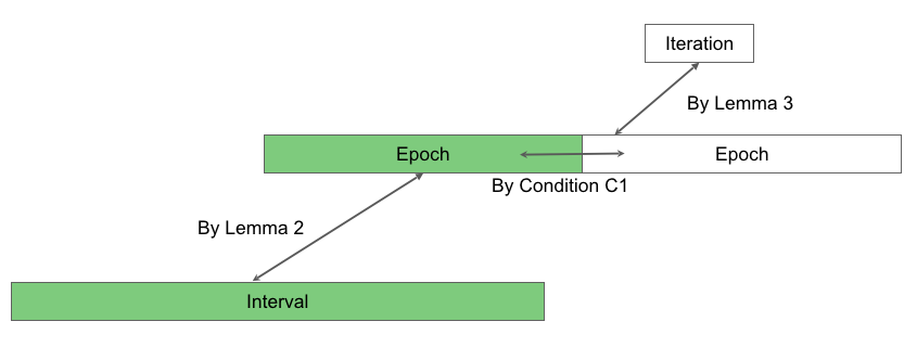
Figure 2: A depiction of the relationship between the good join rate in intervals, epochs, and iterations. Arrows represent that good join rates are within constant factors of each other. Green indicates the most recently-finished epoch and interval being tracked by the committee to obtain $\tilde{J}^{G}_{i}$.

Our approach for estimating the good-ID join rate may be of independent interest for other settings where Assumptions $\text{A}1$ and $\text{A}2$ hold. Therefore, we provide intuition for why they are necessary.

Since good and bad IDs cannot be distinguished with certainty, it is challenging to determine when an epoch begins and ends. Instead, Estimate-GoodJR calculates a lower bound on the number of new good IDs that have joined the system by pessimistically subtracting out the fraction of IDs that could be bad. When this estimate of new good IDs is sufficiently large — that is, when the current interval ends — Estimate-GoodJR “guesses” that at least one epoch has occurred. However, multiple (but still a constant number of) epochs may have actually occurred during this time. Thus, for this approach to yield a constant-factor estimate of $J^{G}_{i}$, the true good join rate cannot have changed “too much" between these epochs, and $\text{A}1$ bounds the amount of such change.

Assumption $\text{A}1$ addresses the good join rate measured over entire, consecutive epochs. But, an interval may end within some epoch $j$. If the good join rate over the portion of epoch $j$ overlapped by the interval deviates by more than a constant factor from $\rho_{j}$, then the estimate will be inaccurate. Assumption $\text{A}2$ ensures that this cannot happen.

3 Theoretical Results

First, we prove that Estimate-GoodJR achieves a constant-factor approximation, $\tilde{J}^{G}_{i}$, to the good-ID join rate $J^{G}_{i}$ (Theorem 1). Define “with high probability” (w.h.p.) to mean with probability at least $1-1/n_{0}^{\gamma}$. All of our arguments hold with high probability over the system lifetime, and they rely on Assumptions $\text{A}1$ and $\text{A}2$. Due to space constraints, we include proofs in AppendixA.

Theorem 1.

For any iteration $i\geq 1$, Estimate-GoodJR provides a constant-factor estimate of the good-ID join rate:

$$c(JE,\texttt{L})J^{G}_{i}\leq\tilde{J}^{G}_{i}\leq c(JE,\texttt{H})J^{G}_{i}$$

where $c(JE,\texttt{L})=\left(\frac{5}{6}\right)\cfrac{c(\mbox{$\text{A}1$, {L}})^{2}c(\mbox{$\text{A}2$, {L}})}{c(\mbox{$\text{A}1$, {U}})}$ and $c(JE,\texttt{H})=\cfrac{5\,c(\mbox{$\text{A}1$, {U}})^{2}c(\mbox{$\text{A}2$, {U}})}{c(\mbox{$\text{A}1$, {L}})}$.

The following theorem bounds the spend rate of ToGCom. We explicitly include the constants from Assumptions $\text{A}1$ and $\text{A}2$.

Theorem 2.

For $\alpha\leq 1/18$, w.h.p. over the system lifetime, ToGCom maintains the Population and Committee invariants and ensures:

$$\mathcal{A}\leq 11d_{2}\left(d_{1}\sqrt{2T(c(JE,\texttt{H})J^{G}+1)}+J^{G}\right)$$

where $d_{1}=\sqrt{2c(JE,\texttt{H})}$ and $d_{2}=\left(\frac{12}{11}+\dfrac{c(\mbox{$\text{A}1$, {U}})c(\mbox{$\text{A}2$, {U}})}{11c(JE,\texttt{L})}\right)$.

The proof of Theorem 2 differs considerably from that of GMCom [21] (see Appendix A.2). We omit our arguments for the Population and Committee invariants, since those are unchanged from [21].

4 Experiments

We now report our empirical results. In Section 4.1, we test assumptions $\text{A}1$ and $\text{A}2$ from Section 2.3. In section 4.2, we measure the computational cost for ToGCom, as a function of the adversarial cost, and compare it against prior PoW based algorithms. Finally, in Section 4.3, we propose and implement several heuristics to improve the performance of ToGCom. All our experiments were written in MATLAB.

Data Sets. Our experiments use data from the following networks:

• Bitcoin: This dataset records the join and departure events of IDs in the Bitcoin network, timestamped to the second, over roughly 7 days [40].

• BitTorrent RedHat: This dataset simulates the join and departure events for the BitTorrent network to obtain a RedHat ISO image. We use the Weibull distribution with shape and scale parameters of 0.59 and 41.0, respectively, from [48].

• Ethereum: This dataset simulates join and departure events of IDs for the Ethereum network. Based on a study in [25], we use the Weibull distribution with shape parameter of 0.52 and scale parameter of 9.8.

• Gnutella: This dataset simulates join and departure events for the Gnutella network. Based on a study in [45], we use an exponential distribution with mean of $2.3$ hours for session time, and Poisson distribution with mean of $1$ ID per second for the arrival rate.

4.1 Testing Assumptions $\text{A}1$ and $\text{A}2$

Experimental Setup. For the Bitcoin network, the system starts with $9212$ IDs, and the join and departure events are based on the dataset from [41]. For the other networks, we initialize the system with $1000$ IDs, and simulate the join and departure events over $1000$ epochs. We assume all joining IDs are good. Every value plotted is the mean of $20$ independent runs.

To test Assumption $\text{A}1$, for each epoch $i\geq 2$, the good join rate in epoch $i$, $\rho_{i}$, is compared to the good join rate in the previous epoch, $\rho_{i-1}$. Results are summarized in the columns labeled $c(\mbox{$\text{A}1$, {L}})$ and $c(\mbox{$\text{A}1$, {U}})$ of Table 1.

To test Assumption $\text{A}2$, for each epoch $i\geq 1$, we consider all periods of time containing at least $2$ good joins events. In particular, we measure the minimum and maximum join rate for epoch $i$, denoted by $\rho_{i}^{min}$ and $\rho_{i}^{max}$, respectively, and compare these values against $\rho_{i}$. The results are presented in Table 1. We have included the corresponding plots in Appendix A.4.

Network	$c(\mbox{$\text{A}1$, {L}})$	$c(\mbox{$\text{A}1$, {U}})$	$c(\mbox{$\text{A}2$, {L}})$	$c(\mbox{$\text{A}2$, {U}})$
Bitcoin	0.1	10	0.0005	30
BitTorrent RedHat	0.125	8	0.067	15
Ethereum Mainnet	0.5	2	0.4	2
Gnutella	0.5	2	0.1	4

Table 1: Constants Assumptions $\text{A}1$ and $\text{A}2$ for Section 4.1

4.2 Evaluating Computational Cost without Heuristics

We now measure the spend rate for ToGCom, focusing solely on the computational cost of solving puzzles. Throughout, we assume a computational cost of $k$ for solving a puzzle of difficulty $k$. We compare the performance of ToGCom against four PoW-based Sybil defense algorithms: GMCom [21], CCom [20], SybilControl [26] and REMP (a name that uses the authors’ initials)[44], summarized below.

GMCom. GMCom is like ToGCom, except for two differences. First, the entrance cost is the maximum of $1$, and the measured join rate in the current iteration divided by an estimate of the good join rate. Second, the estimate of the good join rate is computed via a different (incorrect) heuristic [21].

CCom. CCom is the same as ToGCom except the entrance cost is always 1.

SybilControl. Each ID solves a puzzle to join. Additionally, each ID tests its neighbors with a puzzle every $5$ seconds, removing from its list of neighbors those IDs that fail to provide a solution within a fixed time period. These tests are not coordinated between IDs.

REMP. Each ID solves a puzzle to join. Additionally, each ID must solve puzzles every $W$ seconds. We use Equation (4) from [44] to compute the value of computational spending rate per ID as:

$$\frac{L}{W}=\frac{n}{N_{attacker}}=\frac{T_{max}}{\alpha N}\\$$ (1)

where $L$ is the computational cost to an ID per $W$ seconds, $n$ is the number of IDs that the adversary can add to the system and $N_{attacker}$ is the total number of attackers in the system. Suppose $N$ is the system size, then $N_{attacker}$ is $\alpha N$ since the computational power with the adversary is an $\alpha$ fraction of computational power of the network in our model. Suppose $T_{max}$ is the maximum number of attackers (bad IDs) that can join in $W$ seconds, then to guarantee that the fraction of bad IDs is less than half, $n=T_{max}$. Substituting these values in Equation 1, we can compute total algorithmic spending rate as:

$$\mathcal{A}_{REMP}=(1-\alpha)N\times\frac{L}{W}=\frac{(1-\alpha)T_{max}}{\alpha}$$ (2)

Setup. We assume the good IDs join and depart as described in Section 4.1. We set $\alpha=1/18$, and let $T$ range over $[2^{0},2^{30}]$, where for each value of $T$, the system is simulated for $10,000$ seconds. We also simulate the case $T=0$. We assume that the adversary only solves puzzles to add IDs to the system. For REMP, we consider two values of $T_{max}$, $10^{4}$ and $10^{7}$. Setting $T_{max}=10^{7}$ ensures correctness for all values of $T$ considered, and $T_{max}=10^{4}$ ensures correctness for $T\leq 10^{4}$.

Results. Figure 3 illustrates our results; we omit error bars since they are negligible. The x-axis is the adversarial spending rate, $T$; and the y-axis is the algorithmic spending rate, $\mathcal{A}$. We cut off the plots for REMP-$10^{4}$ and SybilControl, when they can no longer ensure that the fraction of bad IDs is less than $1/2$. We also note that REMP-$10^{7}$ only ensures a minority of bad IDs for up to $T=10^{7}$.

ToGCom always has spend rate as low as the other algorithms for $T\geq 100$, and significantly less than the other algorithms for large $T$, with improvements that grow to about $2$ orders of magnitude. In Section 4.3, our heuristics close this gap, allowing ToGCom to outperform all algorithms for all $T\geq 0$. The spend rate for ToGCom is linear in $\sqrt{T}$, agreeing with our analytical results. We emphasize that the benefits of ToGCom are consistent over four disparate networks. These results illustrate the value of Estimate-GoodJR.

Finally, we note that ToGCom guarantees a fraction of bad IDs no more than $1/6$ for all values of $T$. In contrast, SybilControl and REMP guarantee a fraction of bad IDs less than $1/2$ for the values of $T$ plotted.

For $T\geq 100$, GMCom and CCom perform almost identically. This occurs because of an error in the estimation heuristic of [21], which causes GMCom to incorrectly estimate $J^{G}$, when $T$ is much larger than $J^{G}$ ($J^{G}\approx 10$ in these plots). When the estimate is incorrect, by the specification in [21], the entrance-puzzle hardness is set to $1$, and so GMCom reverts to CCom. Our simulations in [21] assumed knowledge of the good join rate, and thus did not reveal the flaw in GMCom’s estimation method.

4.3 Heuristics

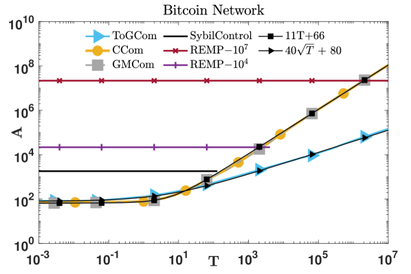
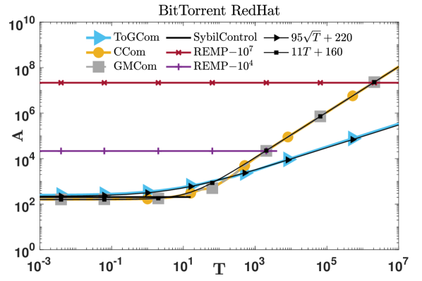
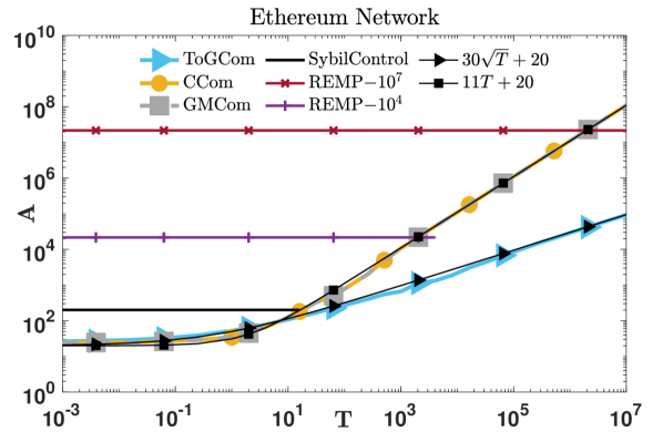
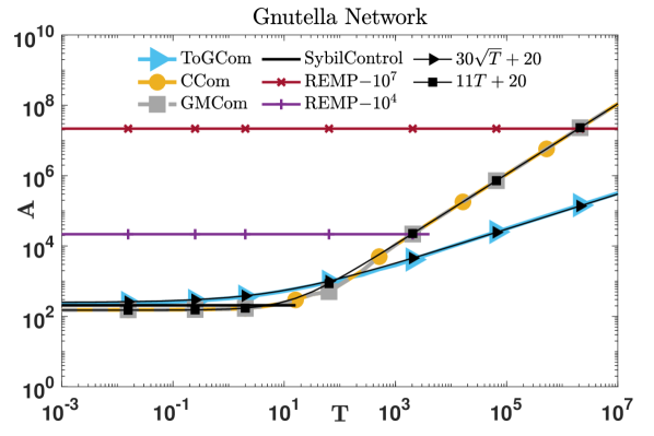
Figure 3: Algorithmic cost versus adversarial cost for ToGCom, GMCom, CCom, SybilControl and REMP.

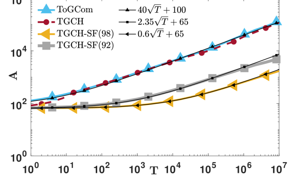
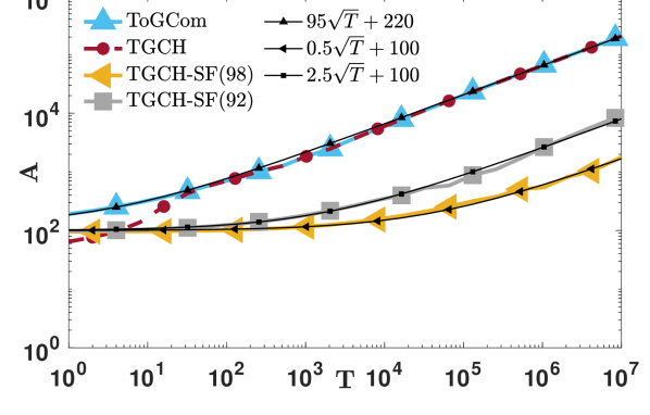
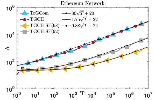
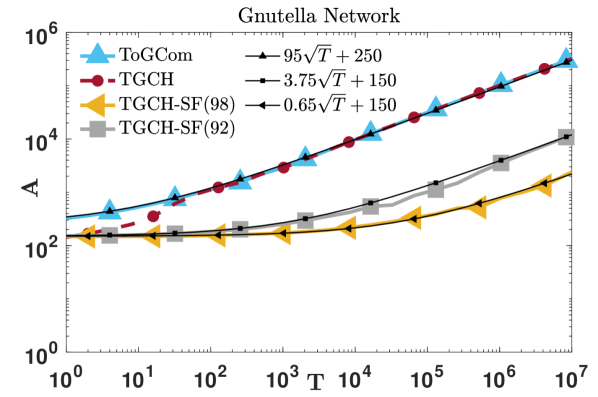
Figure 4: Algorithmic cost versus adversarial cost for ToGCom and heuristics.

Next, we present heuristics to improve the performance of ToGCom. To determine effective heuristics, we focus on two separate costs to good IDs: entrance cost and purge cost. In studying these costs for the Bitcoin network in the absence of an attack, we find that the purge cost dominates and, therefore, we focus on reducing the purge frequency.

Heuristic 1: We use the symmetric difference to determine when to do a purge. Specifically, for iteration $i$, if $|(\mathcal{S}_{\mbox{\tiny cur}}\cup\mathcal{S}_{i-1})-(\mathcal{S}_{\mbox{\tiny cur}}\cap\mathcal{S}_{i-1})|\geq|\mathcal{S}_{i-1}|/11$, then a purge is executed. This ensures that the fraction of bad IDs can increase by no more than in our original specification. Also, it decreases the purge frequency: for example, in the case when some ID joins and departs repeatedly.

Heuristic 2: We use the estimated good-ID join rate, obtained via Estimate-GoodJR, to bound the maximum number of bad IDs that can have joined during an iteration. This allows us to upper-bound the fraction of bad IDs in the system and to purge only when the population invariant is at risk.

Heuristic 3: Recent works have explored the possibility of identifying bad IDs based on the network topology [34, 13]. In our experiments, we focus on SybilFuse [13], which has the probability of correctly classifying an ID as either good or bad as $0.92$ and $0.98$ based on the empirical results from [13], Section IV-B, last paragraph. We assume these values hold and use SybilFuse to diagnose whether a joining ID is good or bad; in the latter case, the ID is refused entry.

We evaluate the performance of these heuristics against ToGCom. The experimental setup is the same as Section 4.2. We define TGCH to be ToGCom using both Heuristic 1 and Heuristic 2. We define TGCH-SF(92) and TGCH-SF(98) to be ToGCom using Heuristics 1 and 2, and also Heuristic 3, with the accuracy parameter of Heuristic 3 as 0.98 and 0.92.

Figure 4 illustrates our results. Note that TGCH-SF(92) and TGCH-SF(98) reduce costs significantly during adversarial attack, with improvements of up to three orders of magnitude during the most significant attack tested. Again, these improvements are consistent across $4$ different types of data sets.

5 Related Work

There is large body of literature on defending against the Sybil attack [10]; for example, see surveys [42, 36, 23], and additional work documenting real-world Sybil attacks [39, 50, 54]. To the best of our knowledge, CCom [20] and GMCom [21] are the first defenses where the algorithmic spend rate grows slowly with the adversarial spend rate.

Domain-Specific Defenses. While PoW-based defenses work in general network settings, domain-specific results for mitigating the Sybil attack have been discovered. In a wireless network with multiple communication channels, Sybil attacks can be mitigated via radio-resource testing which relies on the inability of the adversary to listen to many channels simultaneously [37, 18, 17]. However, this approach may fail if the adversary can monitor most or all of the channels. Furthermore, even in the absence of attack, radio-resource testing requires testing at fixed intervals.

Social Network Properties. Several results that leverage social networks for Sybil resistance [55, 35, 53]. However, social-network information may not be available in many settings. Another idea is to use network measurements to verify the uniqueness of IDs [47, 28, 15], but these techniques rely on accurate measurements of latency, signal strength, or round-trip times, for example, and this may not always be possible. Containment strategies are explored in overlays [9, 46], but these results do not ensure a bound on the fraction of bad IDs.

Proof of Work and Alternatives. As a choice for PoW, computational puzzles provide certain advantages. First, verifying a solution is much easier than solving the puzzle itself. This places the burden of proof on devices that wish to participate in a protocol rather than on a verifier. In contrast, bandwidth-oriented schemes, such as [49], require verification of sufficient number of packets being received before any service is provided; this requires effort by the verifier that is proportional to the number of packets.

A recent alternative to PoW is proof-of-stake (PoS) where security relies on the adversary holding a minority stake in an abstract finite resource [1]. When making a group decision, PoS weights each participant’s vote using its share of a limited resource; for example, the amount of cryptocurrency held by the participant. A well-known example is ALGORAND [16], which employs PoS to form a committee. A hybrid approach using both PoW and PoS has been proposed in the Ethereum system [2].

6 Conclusion

We have presented and analyzed ToGCom, which proposes a novel method for setting the entrance-puzzle difficulty, and for estimating the good-ID join rate. Additionally, we obtained a tight analysis of the asymmetric property. Our proposed heuristics further improve performance, and experiments show that ToGCom decreases computational cost to the good IDs compared to other PoW-based Sybil defenses.

Appendix A Appendix

A.1 Proof of Theorem 1

We say that interval $\tilde{\ell}$ touches an epoch if there is a point in time belonging to both the interval $\tilde{\ell}$ and the interval of time corresponding to the epoch; it does not necessarily mean that $\ell$ completely contains the epoch, or vice versa.

In this section, for any time $t$, let $\mathcal{S}_{t}$ and $\mathcal{G}_{t}$ denote the set of all IDs and set of good IDs, respectively, in the system at time $t$.

Lemma 1.

An interval touches at most two epochs and cannot completely overlap any single epoch.

Proof.

Assume that some interval starts at time $t_{0}$ and touches at least three epochs; we will derive a contradiction. This assumption implies that there is at least one epoch entirely contained within the interval. Consider the first such epoch, and let it start at time $t_{1}\geq t_{0}$ and end at time $t_{2}>t_{1}$. Observe that:

$$|\mathcal{S}_{t_{2}}-\mathcal{S}_{t_{1}}| \geq |\mathcal{G}_{t_{2}}-\mathcal{G}_{t_{1}}|\geq\frac{3}{4}|\mathcal{G}_{t_{2}}|\geq\left(\frac{5}{6}\right)\left(\frac{3}{4}\right)|\mathcal{S}_{t_{2}}|=\frac{5}{8}|\mathcal{S}_{t_{2}}|>\frac{3}{5}|\mathcal{S}_{t_{2}}|$$

where step 2 holds by by the definition of an epoch and step 3 by the Population Invariant. But this is a contradiction since it implies that the interval must end before time $t_{2}$.∎∎

The following lemma considers any interval, $i$, of length $\tilde{\ell}$, where there are $|\mathcal{S}_{\mbox{\tiny cur}}|$ IDs in the system at the end of the interval. By the Population Invariant, the number of good IDs in the system is always at least $(5/6)|\mathcal{S}_{\mbox{\tiny cur}}|$ . Hence, $\frac{|\mathcal{S}_{\mbox{\tiny cur}}|}{\tilde{\ell}}$ is within constant factors of the good join rate during the interval.

Thus, the next lemma shows that the estimate set by the algorithm in interval $i$, $\tilde{J}^{G}_{i}(=\frac{|\mathcal{S}_{\mbox{\tiny cur}}|}{\tilde{\ell}})$, is within constant factors of the good join rate during interval $i$. (See Figure 2).

Lemma 2.

Consider any interval $i\geq 1$, and let epoch $j$ be the most recent epoch that the interval touches. Then:

$$\left(\frac{5}{6}\right)c(\mbox{$\text{A}1$, {L}})c(\mbox{$\text{A}2$, {L}})\rho_{j}\leq\tilde{J}^{G}_{i}\leq 5c(\mbox{$\text{A}1$, {U}})c(\mbox{$\text{A}2$, {U}})\rho_{j}.$$

Proof.

Let interval $i$ be of length $\tilde{\ell}$, and assume there are $|\mathcal{S}_{\mbox{\tiny cur}}|$ IDs in the system at the end of the interval $i$. Then $\tilde{J}^{G}_{i}=\frac{|\mathcal{S}_{\mbox{\tiny cur}}|}{\tilde{\ell}}$. There are three cases.

Case 1: Interval $i$ touches only a single epoch where the epoch begins at $t_{0}$, the interval begins at $t_{1}$, and the interval ends at $t_{2}$. By assumption $\text{A}2$, we have:

$$c(\mbox{$\text{A}2$, {L}})\rho_{j}\leq\frac{|\mathcal{G}_{t_{2}}-\mathcal{G}_{t_{1}}|}{t_{2}-t_{1}}\leq c(\mbox{$\text{A}2$, {U}})\rho_{j}$$

and by the Population Invariant and the specification of an interval:

$$\left(\frac{2}{5}\right)|\mathcal{S}_{t_{2}}|\leq\left(\frac{3}{5}-\frac{1}{6}\right)|\mathcal{S}_{t_{2}}|\leq|\mathcal{G}_{t_{2}}-\mathcal{G}_{t_{1}}|\leq\left(\frac{3}{5}\right)|\mathcal{S}_{t_{2}}|.$$

Therefore, we have:

$$\left(\frac{5}{3}\right)c(\mbox{$\text{A}2$, {L}})\rho_{j}\leq\frac{|\mathcal{S}_{t_{2}}|}{t_{2}-t_{1}}\leq\left(\frac{5}{2}\right)c(\mbox{$\text{A}2$, {U}})\rho_{j}$$

Case 2: The interval touches epochs $i-1$ and $i$ and there are at least $2$ good ID join events in each epoch. Let epoch $i-1$ start at time $t_{0}$ and end at $t_{2}$ (and so epoch $i$ starts at $t_{2}$), and let the interval start at time $t_{1}\geq t_{0}$ and end at $t_{3}\geq t_{2}$. By Assumptions $\text{A}1$ and A2, we have:

$$c(\mbox{$\text{A}1$, {L}})c(\mbox{$\text{A}2$, {L}})\rho_{j}\leq\frac{|\mathcal{G}_{t_{3}}-\mathcal{G}_{t_{1}}|}{t_{3}-t_{1}}\leq c(\mbox{$\text{A}1$, {U}})c(\mbox{$\text{A}2$, {U}})\rho_{j}$$

and by the Population Invariant and the specification of an interval:

$$\left(\frac{2}{5}\right)|\mathcal{S}_{t_{3}}|\leq\left(\frac{3}{5}-\frac{1}{6}\right)|\mathcal{S}_{t_{3}}|\leq|\mathcal{G}_{t_{3}}-\mathcal{G}_{t_{1}}|\leq\left(\frac{3}{5}\right)|\mathcal{S}_{t_{3}}|.$$

Therefore, we have:

$$\left(\frac{5}{3}\right)c(\mbox{$\text{A}1$, {L}})c(\mbox{$\text{A}2$, {L}})\rho_{j}\leq\frac{|\mathcal{S}_{t_{3}}|}{t_{3}-t_{1}}\leq\left(\frac{5}{2}\right)c(\mbox{$\text{A}1$, {U}})c(\mbox{$\text{A}2$, {U}})\rho_{j}$$

which we refer to as the Case-2 Equation.

Case 3: The interval touches epochs $j-1$ and $j$, and w.l.o.g. we have a single good join event in the portion of epoch $j-1$ that overlaps the interval; denote the length of this overlap by $\lambda^{\prime}>0$. As with Case 2, let epoch $j-1$ start at time $t_{0}$ and end at $t_{2}$ (and so epoch $j$ starts at $t_{2}$), and let the interval start at time $t_{1}\geq t_{0}$ and end at $t_{3}\geq t_{2}$.

Observe that the single good join event in epoch $j-1$ increases the numerator of the bounded quantity in the Case-2 Equation by $1$, and so twice the upper bound in Case 2 suffices here. The denominator increases by $\lambda^{\prime}$, where $\lambda^{\prime}\leq t_{3}-t_{1}$, so half the lower bound in Case 2 suffices. This implies:

$$\left(\frac{5}{6}\right)c(\mbox{$\text{A}1$, {L}})c(\mbox{$\text{A}2$, {L}})\rho_{j}\leq\frac{|\mathcal{S}_{t_{3}}|}{t_{3}-t_{1}}\leq 5c(\mbox{$\text{A}1$, {U}})c(\mbox{$\text{A}2$, {U}})\rho_{j}$$

∎∎

Lemma 3.

For any epoch $j\geq 1$, and any iteration $i\geq 1$ that epoch $j$ touches:

$$c(\mbox{$\text{A}1$, {L}})J^{G}_{i}\leq\rho_{j}\leq c(\mbox{$\text{A}1$, {U}})J^{G}_{i}$$

Proof.

By Lemma 1, iteration $j$ touches at most two epochs, say epochs $j-1$ and $j$. Thus, by definition of $J^{G}_{i}$, for some $\lambda_{1},\lambda_{2}\geq 0$, $\lambda_{1}+\lambda_{2}=1$:

$$J^{G}_{i}=\lambda_{1}\rho_{j-1}+\lambda_{2}\rho_{j}\leq\lambda_{1}\left(\frac{\rho_{j}}{c(\mbox{$\text{A}1$, {L}})}\right)+\lambda_{2}\rho_{j}\leq\frac{\rho_{j}}{c(\mbox{$\text{A}1$, {L}})}$$

The second step above holds by assumption $\text{A}1$. The last step holds since $\lambda_{1}+\lambda_{2}=1$ and $c(\mbox{$\text{A}1$, {L}})\leq 1$. A similar derivation yields that $J^{G}_{i}\geq\frac{\rho_{j}}{c(\mbox{$\text{A}1$, {U}})}$. Together this implies that: $c(\mbox{$\text{A}1$, {L}})J^{G}_{i}\leq\rho_{j}\leq c(\mbox{$\text{A}1$, {U}})J^{G}_{i}.$ ∎∎

We can now prove Theorem 1, restate below.

Theorem 1.

For any iteration $i\geq 1$, Estimate-GoodJR provides a constant-factor estimate of the good-ID join rate:

$$c(JE,\texttt{L})J^{G}_{i}\leq\tilde{J}^{G}_{i}\leq c(JE,\texttt{H})J^{G}_{i}$$

where $c(JE,\texttt{L})=\left(\frac{5}{6}\right)\cfrac{c(\mbox{$\text{A}1$, {L}})^{2}c(\mbox{$\text{A}2$, {L}})}{c(\mbox{$\text{A}1$, {U}})}$ and $c(JE,\texttt{H})=\cfrac{5\,c(\mbox{$\text{A}1$, {U}})^{2}c(\mbox{$\text{A}2$, {U}})}{c(\mbox{$\text{A}1$, {L}})}$.

Proof.

The estimate $\tilde{J}^{G}_{i}$ used in iteration $i$ corresponds to the most recent interval that completed before iteration $i$ started. Let epoch $j$ be the most recent epoch that touches this interval. By Lemma 2:

$$\left(\frac{5}{6}\right)c(\mbox{$\text{A}1$, {L}})c(\mbox{$\text{A}2$, {L}})\rho_{j}\leq\tilde{J}^{G}_{i}\leq 5\,c(\mbox{$\text{A}1$, {U}})c(\mbox{$\text{A}2$, {U}})\rho_{j}.$$

Epoch $j$ may end prior to the start of iteration $i$; that is, epoch $j$ may not necessarily touch iteration $i$. In this case, note that by Lemma 1, the current interval touches epoch $j+1$ and must end before epoch $j+1$ ends. This fact, along with the observation that the current interval touches iteration $i$, implies that epoch $j+1$ touches iteration $i$.

By the above, we know that either epoch $j+1$ or epoch $j$ touches iteration $i$. Lemma 3 implies:

$$c(\mbox{$\text{A}1$, {L}})J^{G}_{i}\leq\rho_{j}\leq c(\mbox{$\text{A}1$, {U}})J^{G}_{i}$$

or

$$c(\mbox{$\text{A}1$, {L}})J^{G}_{i}\leq\rho_{j+1}\leq c(\mbox{$\text{A}1$, {U}})J^{G}_{i}.$$

To employ our top-most equation, we use $\text{A}1$ to derive:

$$\rho_{j+1}/c(\mbox{$\text{A}1$, {U}})\leq\rho_{j}\leq\rho_{j+1}/c(\mbox{$\text{A}1$, {L}})$$

and then plug into our top-most equation, we have:

$$\left(\frac{5}{6}\right)\frac{c(\mbox{$\text{A}1$, {L}})^{2}c(\mbox{$\text{A}2$, {L}})}{c(\mbox{$\text{A}1$, {U}})}J^{G}_{i}\leq\tilde{J}^{G}_{i}\leq\frac{5\,c(\mbox{$\text{A}1$, {U}})^{2}c(\mbox{$\text{A}2$, {U}})}{c(\mbox{$\text{A}1$, {L}})}J^{G}_{i}$$

∎∎

A.2 Proof of Theorem 2

We make use of the following algebraic fact that follows from the Cauchy-Schwartz inequality.

Lemma 4.

Let $n$ be a positive number, and for all $1\leq i\leq n$, $s_{i}\geq 0$ and let $S=\sum_{i=1}^{n}s_{i}$. Then

$$\sum_{i=1}^{n}s_{i}^{2}\geq S^{2}/n$$

Proof.

Let $u$ be a vector of length $n$ with for all $1\leq i\leq n$, $u[i]=s_{i}$, and let $v$ be a vector of length $n$ with, for all $1\leq i\leq n$, $v[i]=1$. Then by Cauchy-Schwartz:

$$|\langle u,v\rangle|^{2} \leq \langle u,u\rangle\cdot\langle v,v\rangle$$

$$S^{2} \leq \left(\sum_{i=1}^{n}s_{i}^{2}\right)\cdot n$$

Rearranging completes the proof.∎∎

Let $\mathcal{T}_{i}$ denote the cost to the adversary over iteration $i$ divided by the length of iteration $i$. Let $J^{B}_{i}$ be the join rate of bad IDs during iteration $i$. Recall that $c(JE,\texttt{H})J^{G}_{i}=\frac{5c(\mbox{$\text{A}1$, {U}})^{2}c(\mbox{$\text{A}2$, {U}})}{c(\mbox{$\text{A}1$, {L}})}$.

Lemma 5.

For any iteration $i>1$,

$$J^{B}_{i}\leq d_{1}\sqrt{T_{i}(J^{G}_{i}+1)}$$

where $d_{1}=\sqrt{2c(JE,\texttt{H})}$.

Proof.

For simplicity, we normalize time units so that $\ell_{i}=1$. Partition iteration $i$ from left to right into sub-iterations, all of length $1/\tilde{J}^{G}_{i}$, except the last, which is of length at most $1/\tilde{J}^{G}_{i}$. We lower bound the cost paid by the adversary for joins by pessimistically assuming that only bad IDs are counted when computing entrance costs. For $1\leq x\leq\lceil\tilde{J}^{G}_{i}\rceil$, let $j_{x}$ be the total number of bad IDs that join in sub-iteration $x$. Since $\sum_{y=1}^{j_{x}}y=(j_{x}+1)j_{x}/2\geq(j_{x})^{2}/2$, the total entrance cost paid by bad IDs is at least $(1/2)\sum_{x=1}^{\lceil\tilde{J}^{G}_{i}\rceil}(j_{x})^{2}$.

zSince $\sum_{x=1}^{\lceil\tilde{J}^{G}_{i}\rceil}j_{x}=J^{B}_{i}$, by applying Lemma 4, we have:

$$T_{i}\geq\frac{1}{2}\sum_{x=1}^{\lceil\tilde{J}^{G}_{i}\rceil}(j_{x})^{2}\geq\frac{(J^{B}_{i})^{2}}{2(\lceil\tilde{J}^{G}_{i}\rceil)}$$

Cross-multiplying and taking the square root, we get:

$$J^{B}_{i} \leq \sqrt{2T_{i}\lceil\tilde{J}^{G}_{i}\rceil}\leq\sqrt{2T_{i}(\tilde{J}^{G}_{i}+1)}\leq\sqrt{2T_{i}\left(c(JE,\texttt{H})J^{G}_{i}+1\right)}$$

where the second step follows from noting that $\lceil x\rceil\leq x+1$ for all $x$, and the final step follows from Lemma 1 which states that:

$$\tilde{J}^{G}_{i}\leq\frac{5c(\mbox{$\text{A}1$, {U}})^{2}c(\mbox{$\text{A}2$, {U}})}{c(\mbox{$\text{A}1$, {L}})}J^{G}_{i}=c(JE,\texttt{H})J^{G}_{i}$$

which yields the lemma statement. ∎∎

Lemma 6.

Let $\mathcal{A}_{i}$ be the average spend rate for the algorithm in any iteration $i>1$. Then, $\mathcal{A}_{i}\leq\frac{d_{2}|S_{i-1}|}{\ell_{i}}$, where $d_{2}=\left(\frac{12}{11}+\frac{c(\mbox{$\text{A}1$, {U}})c(\mbox{$\text{A}2$, {U}})}{11c(JE,\texttt{L})}\right)$.

Proof.

For simplicity, we first normalize time units so that $\ell_{i}=1$. Partition iteration $i$ from left to right into sub-iterations, all of length $1/J^{G}_{i}$, except the last, which is of length at most $1/J^{G}_{i}$.

The spend rate for the algorithm due to purge costs is $|S_{i-1}|$.

For entrance costs, note the following two facts. First, by Assumptions A1 and A2, there are at most $c(\mbox{$\text{A}1$, {U}})c(\mbox{$\text{A}2$, {U}})$ good IDs in any sub-iteration (note that a sub-iteration might span two epochs). Second, the entrance cost for any good ID is $1$ plus the number of join events over the past $1/\tilde{J}^{G}_{i}$ seconds. By Theorem 1, $1/\tilde{J}^{G}_{i}\leq 1/(c(JE,\texttt{L})J^{G}_{i})$, and so the entrance cost is at most $1$ plus the number of join events over the past $1/c(JE,\texttt{L})$ sub-iterations; that is $1+c(\mbox{$\text{A}1$, {U}})c(\mbox{$\text{A}2$, {U}})/c(JE,\texttt{L})$.

By these two facts, and by the fact that there are at most $|S_{i-1}|/11$ join events in an iteration, the total entrance costs paid by good IDs in iteration $i$ is at most:

$$\left(1+\frac{c(\mbox{$\text{A}1$, {U}})c(\mbox{$\text{A}2$, {U}})}{c(JE,\texttt{L})}\right)\left(\frac{|S_{i-1}|}{11}\right).$$

Adding the bounds for both entrance and purge costs and dividing by the value of $\ell_{i}$ yields a total cost of at most:

$$\frac{|S_{i-1}|}{\ell_{i}}\left(\frac{12}{11}+\frac{c(\mbox{$\text{A}1$, {U}})c(\mbox{$\text{A}2$, {U}})}{11c(JE,\texttt{L})}\right)$$

∎∎

Let $\mathcal{I}$ be any subset of iterations that for integers $x$ and $y$, $1\leq x\leq y$, contains every iteration with index between $x$ and $y$ inclusive. Let $\delta(\mathcal{I})$ be $|S_{x}-S_{y}|$; and let $\Delta(\mathcal{I})$ be $\delta(\mathcal{I})$ divided by the length of $\mathcal{I}$. Let $\mathcal{A}_{\mathcal{I}}$ and $T_{\mathcal{I}}$ be the algorithmic and adversarial spend rates over $\mathcal{I}$; and let $J^{G}_{\mathcal{I}}$ be the good join rate over all of $\mathcal{I}$. Then we have the following lemma.

Lemma 7.

For any subset of contiguous iterations, $\mathcal{I}$,which starts after iteration $1$, the algorithmic spending rate over $\mathcal{I}$ is at most:

$$11d_{2}\left(2\Delta(\mathcal{I})+d_{1}\sqrt{2T_{\mathcal{I}}(c(JE,\texttt{H})J^{G}_{\mathcal{I}}+1)}+J^{G}_{\mathcal{I}}\right).$$

Proof.

Let $D_{i}$ be the departure rate of both good and bad IDs during iteration $i$. By Lemma 6 and the assumptions for when a purge occurs, we have that:

$$\sum_{i\in\mathcal{I}}\mathcal{A}_{i}\ell_{i} \leq d_{2}\sum_{i\in\mathcal{I}}|S_{i-1}|$$

$$\leq 11d_{2}\sum_{i\in\mathcal{I}}(D_{i}+J^{B}_{i}+J^{G}_{i})\ell_{i}$$

$$\leq 11d_{2}\Bigg{(}2\delta(\mathcal{I})+\sqrt{\sum_{i\in\mathcal{I}}2T_{i}\ell_{i}\sum_{i\in\mathcal{I}}(c(JE,\texttt{H})J^{G}_{i}+1)\ell_{i}}+\sum_{i\in\mathcal{I}}J^{G}_{i}\ell_{i}\Bigg{)}$$

The second line in the above follows from the fact that every ID that departs must have departed from the set of IDs in the system at the start of $\mathcal{I}$ or else must have been an ID that joined during $\mathcal{I}$. The last line follows from the Lemma 5 bound on $J^{B}_{i}$, and noting that $\ell_{i}=\sqrt{\ell^{2}_{i}}$. Finally, the last line follows from Cauchy-Schwarz Inequality.

Dividing both sides of the above inequality by $\sum_{i\in\mathcal{I}}\ell_{i}$ and recalling that $d_{1}=\sqrt{2c(JE,\texttt{H})}$, completes the proof. ∎∎

The above result is more general than we need, but Theorem 2 follows from Lemma 7 by noting that $\Delta(\mathcal{I})=0$ when $\mathcal{I}$ is all iterations, since the system is initially empty. We state an interesting corollary implied by Theorem 2.

Corollary 1.

For $\alpha\leq 1/18$, with error probability polynomially small in $n_{0}$ over the system lifetime, and for any subset of contiguous iterations $\mathcal{I}$, ToGCom has an algorithmic spending rate of $O\left(\sqrt{T_{\mathcal{I}}\,(J^{G}_{\mathcal{I}}+1)}+\Delta(\mathcal{I})+J^{G}_{\mathcal{I}}\right)$.

This shows that the spending rate for the algorithm remains small, even when focusing on just a subset of iterations. To understand why this is important, consider a long-lived system which suffers a single, significant attack for a small number of iterations, after which there are no more attacks. The cost of any defense may be small when amortized over the lifetime of the system, but this does not give a useful guarantee on performance during the time of attack.

A.3 GMCom with close Join Events

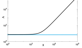
Figure 5: Comparison of algorithmic spend rate for CCom and GMCom as join event grows closer to beginning of an epoch.

Experimetal Setup. We simulate CCom and GMCom over a system that always consists of $10,000$ good IDs. During the lifetime of the system, new good IDs join/depart at a constant rate of one ID per time step. The departing ID is chosen uniformly at random from the set of IDs that joined before the current iteration. We run for 2 iterations and then have a single join event in the third iteration. This last join event occurs arbitrarily close to second to last join event which ended the previous iteration.

Let the time between the second to last and the last join event be $1/X$, for some value $X>0$. Thus, as $X$ increases, these two last join events become closer together. For $X\in\{2^{0},2^{1},...,2^{30}\}$, we compute the spend rate for CCom and GMCom.

Figure 5 illustrates our results. As can be seen, as $X$ increases, the algorithmic spend rate, $\mathcal{A}$, increases linearly for GMCom, whereas for CCom it remains constant. This increase in the spend rate for GMCom occurs solely because of the increasing entrance cost for the very last good join event.

A.4 Plots from Experiments of Section 4.1

In Figure 6, we present the plots from our experiments testing Assumptions $\text{A}1$ and $\text{A}2$. These are used to derive the values presented in Table 1.

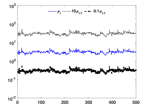
(a) (a)

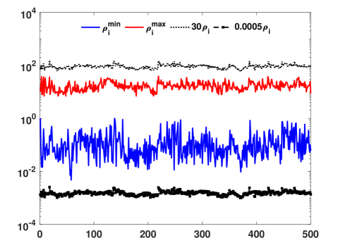
(b) (b)

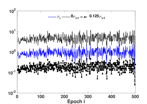
(c) (c)

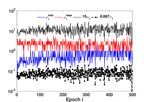
(d) (d)

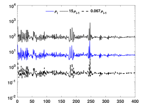
(e) (e)

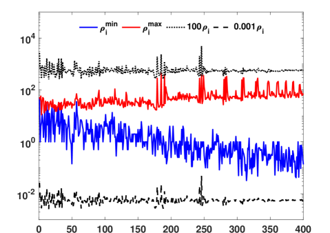
(f) (f)

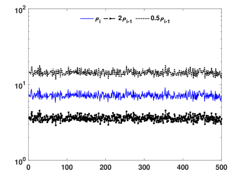
(g) (g)

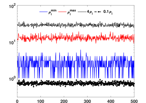
(h) (h)

Figure 6: Testing Assumptions $\text{A}1$ and $\text{A}2$ for (a) & (b) Bitcoin Network, (c) & (d) BitTorrent Redhat, (e) & (f) Ethereum Network, and (g) & (h) Gnutella Network.

References

- [1] Abraham, I., Malkhi, D.: The Blockchain Consensus Layer and BFT. Bulletin of the EATCS: Distributed Computing Column (2017)
- [2] Alyssa Hertig: Ethereum’s Big Switch: The New Roadmap to Proof-of-Stake, www.coindesk.com/ethereums-big-switch-the-new-roadmap-to-proof-of-stake/
- [3] Andrychowicz, M., Dziembowski, S.: PoW-Based Distributed Cryptography with No Trusted Setup. In: Annual Cryptology Conference. pp. 379–399. Springer (2015)
- [4] BitcoinWiki: BitcoinWiki Network, https://en.bitcoin.it/wiki/Network\#Standard_relaying
- [5] Blockstack: Blockstack: The New Decentralized Internet (2017), https://blockstack.org/
- [6] Borisov, N.: Computational Puzzles As Sybil Defenses. In: Proceedings of the Sixth IEEE International Conference on Peer-to-Peer Computing. pp. 171–176 (2006)
- [7] CoinDesk: Think Tank Reignites Debate Over Bitcoin Mining’s Environmental Effects. http://www.coindesk.com/think-tank-debate-bitcoin-mining-environment/ (2015)
- [8] Croman, K., Decker, C., Eyal, I., Gencer, A.E., Juels, A., Kosba, A., Miller, A., Saxena, P., Shi, E., Sirer, E.G., et al.: On scaling decentralized blockchains. In: International Conference on Financial Cryptography and Data Security. pp. 106–125. Springer (2016)
- [9] Danezis, G., Lesniewski-laas, C., Kaashoek, M.F., Anderson, R.: Sybil-Resistant DHT Routing. In: Proceedings of the European Symposium On Research In Computer Security (ESORICS). pp. 305–318 (2005)
- [10] Douceur, J.: The Sybil Attack. In: Proceedings of the Second International Peer-to-Peer Symposium (IPTPS). pp. 251–260 (2002)
- [11] Dwork, C., Naor, M.: Pricing via Processing or Combatting Junk Mail. In: Proceedings of the Annual International Cryptology Conference on Advances in Cryptology. pp. 139–147 (1993)
- [12] Feng, W., Kaiser, E., Feng, W., Luu, A.: The Design and Implementation of Network Puzzles. In: Proceedings of the Annual Joint Conference of IEEE Computer and Communications Societies (INFOCOM). pp. 2372–2382 (2005)
- [13] Gao, P., Wang, B., Gong, N.Z., Kulkarni, S.R., Thomas, K., Mittal, P.: Sybilfuse: Combining local attributes with global structure to perform robust sybil detection. In: 2018 IEEE Conference on Communications and Network Security (CNS). pp. 1–9 (2018), https://www.princeton.edu/~pmittal/publications/sybilfuse-cns18.pdf
- [14] Garay, J., Kiayias, A., Leonardos, N.: The Bitcoin Backbone Protocol: Analysis and Applications. In: Proceedings of 34th Annual International Conference on the Theory and Applications of Cryptographic Techniques (EUROCRYPT). pp. 281–310 (2015)
- [15] Gil, S., Kumar, S., Mazumder, M., Katabi, D., Rus, D.: Guaranteeing Spoof-Resilient Multi-Robot Networks. In: Proceedings of Robotics: Science and Systems. Rome, Italy (July 2015)
- [16] Gilad, Y., Hemo, R., Micali, S., Vlachos, G., Zeldovich, N.: Algorand: Scaling Byzantine Agreements for Cryptocurrencies. In: Proceedings of the 26th Symposium on Operating Systems Principles (SOSP). pp. 51–68 (2017)
- [17] Gilbert, S., Newport, C., Zheng, C.: Who Are You? Secure Identities in Ad Hoc Networks. In: Proceedings of the International Symposium on Distributed Computing (DISC). pp. 227–242 (2014)
- [18] Gilbert, S., Zheng, C.: SybilCast: Broadcast on the Open Airwaves. In: Proceedings of the Annual ACM Symposium on Parallelism in Algorithms and Architectures (SPAA). pp. 130–139 (2013)
- [19] Green, J., Juen, J., Fatemieh, O., Shankesi, R., Jin, D., Gunter, C.A.: Reconstructing Hash Reversal Based Proof of Work Schemes. In: Proceedings of the 4th USENIX Conference on Large-scale Exploits and Emergent Threats (LEET). pp. 10–10 (2011)
- [20] Gupta, D., Saia, J., Young, M.: Proof of Work Without All the Work. In: Proceedings of the International Conference on Distributed Computing and Networking (ICDCN) (2018)
- [21] Gupta, D., Saia, J., Young, M.: Peace through superior puzzling: An asymmetric sybil defense. In: 33rd IEEE International Parallel and Distributed Processing Symposium (IPDPS) (2019)
- [22] Hou, R., Jahja, I., Luu, L., Saxena, P., Yu, H.: Randomized view reconciliation in permissionless distributed systems. IEEE INFOCOM 2018-IEEE Conference on Computer Communications pp. 2528–2536 (2018)
- [23] John, R., Cherian, J.P., Kizhakkethottam, J.J.: A Survey of Techniques to Prevent Sybil Attacks. In: Proc. of the Intl. Conference on Soft-Computing and Networks Security (ICSNS). pp. 1–6 (2015)
- [24] Kaiser, E., Feng, W.c.: Mod_kaPoW: Mitigating DoS with Transparent Proof-of-Work. In: Proc. of the 2007 ACM CoNEXT Conference. pp. 74:1–74:2 (2007)
- [25] Kim, S.K., Ma, Z., Murali, S., Mason, J., Miller, A., Bailey, M.: Measuring ethereum network peers. In: Proceedings of the Internet Measurement Conference 2018. pp. 91–104 (2018)
- [26] Li, F., Mittal, P., Caesar, M., Borisov, N.: SybilControl: Practical Sybil Defense with Computational Puzzles. In: Proceedings of the Seventh ACM Workshop on Scalable Trusted Computing. pp. 67–78 (2012)
- [27] Litecoin: Litecoin: Global Decentralized Currency (2017), https://litecoin.org/
- [28] Liu, Y., Bild, D.R., Dick, R.P., Mao, Z.M., Wallach, D.S.: The Mason Test: A Defense Against Sybil Attacks in Wireless Networks Without Trusted Authorities. IEEE Transactions on Mobile Computing 14(11), 2376–2391 (2015)
- [29] Luu, L., Narayanan, V., Zheng, C., Baweja, K., Gilbert, S., Saxena, P.: A Secure Sharding Protocol For Open Blockchains. In: Proc. of the 2016 ACM SIGSAC Conference on Computer and Communications Security (CCS). pp. 17–30 (2016)
- [30] Martinovic, I., Zdarsky, F.A., Wilhelm, M., Wegmann, C., Schmitt, J.B.: Wireless Client Puzzles in IEEE 802.11 Networks: Security by Wireless. In: Proc. of the First ACM Conference on Wireless Network Security. pp. 36–45. WiSec ’08 (2008)
- [31] Ars Technica: Mining bitcoins takes power, but is it an Environmental Disaster? http://arstechnica.com/business/2013/04/mining-bitcoins-takes-power-but-is-it-an-environmental-disaster (2013)
- [32] The Economist: Why bitcoin uses so much energy. https://www.economist.com/the-economist-explains/2018/07/09/why-bitcoin-uses-so-much-energy (2018)
- [33] Miller, A., Litton, J., Pachulski, A., Spring, N., Gupta, N., Levin, D., Bhattacharjee, B.: Discovering Bitcoin’s Public Topology and Influential Nodes (2015), http://cs.umd.edu/projects/coinscope/coinscope.pdf
- [34] Misra, S., Tayeen, A.S.M., Xu, W.: Sybilexposer: An effective scheme to detect sybil communities in online social networks. In: 2016 IEEE International Conference on Communications (ICC). pp. 1–6. IEEE (2016)
- [35] Mohaisen, A., Hollenbeck, S.: Improving Social Network-Based Sybil Defenses by Rewiring and Augmenting Social Graphs. In: Proceedings of the International Workshop on Information Security Applications (WISA). pp. 65–80 (2014)
- [36] Mohaisen, A., Kim, J.: The Sybil Attacks and Defenses: A Survey. Smart Computing Review 3(6), 480–489 (2013)
- [37] Mónica, D., Leitao, L., Rodrigues, L., Ribeiro, C.: On the Use of Radio Resource Tests in Wireless Ad-Hoc Networks. In: Proceedings of the 3rd Workshop on Recent Advances on Intrusion-Tolerant Systems. pp. F21–F26 (2009)
- [38] Nakamoto, S.: Bitcoin: A Peer-to-Peer Electronic Cash System (2008), http://bitcoin.org/bitcoin.pdf
- [39] Neudecker, T.: Bitcoin Cash (BCH) Sybil Nodes on the Bitcoin Peer-to-Peer Network (2017), http://dsn.tm.kit.edu/publications/files/332/bch_sybil.pdf
- [40] Neudecker, T.: Personal correspondence (2019)
- [41] Neudecker, T., Andelfinger, P., Hartenstein, H.: Timing analysis for inferring the topology of the bitcoin peer-to-peer network. In: Proceedings of the 13th IEEE International Conference on Advanced and Trusted Computing (ATC) (July 2016)
- [42] Newsome, J., Shi, E., Song, D., Perrig, A.: The Sybil Attack in Sensor Networks: Analysis & Defenses. In: Proceedings of the 3rd International Symposium on Information Processing in Sensor Networks (IPSN). pp. 259–268 (2004)
- [43] Parno, B., Wendlandt, D., Shi, E., Perrig, A., Maggs, B., Hu, Y.C.: Portcullis: Protecting Connection Setup from Denial-of-Capability Attacks. ACM SIGCOMM Computer Communication Review 37(4), 289–300 (2007)
- [44] Rowaihy, H., Enck, W., Mcdaniel, P., La Porta, T.: Limiting sybil attacks in structured peer-to-peer networks. In: Proceedings of IEEE Infocom Mini-Symposium. IEEE Press, Washington, DC, USA. pp. 1201–1206 (2005)
- [45] Rowaihy, H., Enck, W., McDaniel, P., La Porta, T.: Limiting sybil attacks in structured p2p networks. In: IEEE International Conference on Computer Communications (INFOCOM). pp. 2596–2600 (2007)
- [46] Scheideler, C., Schmid, S.: A Distributed and Oblivious Heap. In: Proceedings of the 36th Internatilonal Collogquium on Automata, Languages and Programming: Part II. pp. 571–582. ICALP ’09 (2009)
- [47] Sherr, M., Blaze, M., Loo, B.T.: Veracity: Practical Secure Network Coordinates via Vote-based Agreements. In: Proceedings of the USENIX Annual Technical Conference. pp. 13 –13 (2009)
- [48] Stutzbach, D., Rejaie, R.: Understanding Churn in Peer-to-peer Networks. In: Proceedings of the 6th ACM SIGCOMM Conference on Internet Measurement (IMC). pp. 189–202. ACM, New York, NY, USA (2006), http://doi.acm.org/10.1145/1177080.1177105
- [49] Walfish, M., Vutukuru, M., Balakrishnan, H., Karger, D., Shenker, S.: DDoS Defense by Offense. ACM Transactions on Computer Systems 28(1), 3 (2010)
- [50] Wang, L., Kangasharju, J.: Real-World Sybil Attacks in BitTorrent Mainline DHT. In: IEEE Global Communications Conference (GLOBECOM). pp. 826–832 (2012)
- [51] Wang, X., Reiter, M.K.: Defending Against Denial-of-Service Attacks with Puzzle Auctions. In: Proc. of the IEEE Symposium on Security and Privacy. p. 78 (2003)
- [52] Waters, B., Juels, A., Halderman, A., Felten, E.: New Client Puzzle Outsourcing Techniques for DoS Resistance. In: Proceedings of the 11th ACM Conference on Computer and Communications Security (CCS). pp. 246–256 (2004)
- [53] Wei, W., Xu, F., Tan, C.C., Li, Q.: SybilDefender: A Defense Mechanism for Sybil Attacks in Large Social Networks. IEEE Transactions on Parallel & Distributed Systems 24(12), 2492–2502 (2013)
- [54] Yang, Z., Wilson, C., Wang, X., Gao, T., Zhao, B.Y., Dai, Y.: Uncovering Social Network Sybils in the Wild. In: Proceedings of the 2011 ACM SIGCOMM Conference on Internet Measurement Conference (IMC). pp. 259–268 (2011)
- [55] Yu, H., Kaminsky, M., Gibbons, P.B., Flaxman, A.: SybilGuard: Defending Against Sybil Attacks via Social Networks. Proceedings of the 2006 Conference on Applications, Technologies, Architectures, and Protocols for Computer Communications (SIGCOMM) 36, 267–278 (Aug 2006)