Abstract

Accelerated proximal gradient methods have recently been developed for solving quasi-static incremental problems of elastoplastic analysis with some different yield criteria. It has been demonstrated through numerical experiments that these methods can outperform conventional optimization-based approaches in computational plasticity. However, in literature these algorithms are described individually for specific yield criteria, and hence there exists no guide for application of the algorithms to other yield criteria. This short paper presents a general form of algorithm design, independent of specific forms of yield criteria, that unifies the existing proximal gradient methods. Clear interpretation is also given to each step of the presented general algorithm so that each update rule is linked to the underlying physical laws in terms of mechanical quantities.

Keywords

Elastoplastic analysis; incremental problem; nonsmooth convex optimization; first-order optimization method; proximal gradient method.

1 Introduction

In these 15 years, it has become a trend to apply constrained convex optimization approaches to diverse problems in computational plasticity. Particularly, second-order cone programming (SOCP) and semidefinite programming (SDP) have drawn considerable attention; see [4, 36, 20, 22, 23, 17, 16] for SOCP approaches, [3, 5, 11, 35, 18, 24, 21] for SDP approaches, and [31] for recent survey on numerical methods in plasticity. Most of these approaches make use of interior-point methods; particularly, it is known that primal-dual interior-point methods can solve SOCP and SDP problems in polynomial time, and in practice require a reasonably small number of iterations [1].

Recently, accelerated proximal gradient methods have been developed for solving quasi-static incremental problems in elastoplastic analysis of trusses [15] and continua with the von Mises [32] and Tresca [33] yield criteria. In contrast to SOCP and SDP approaches, these methods solve unconstrained nonsmooth convex optimization formulations of incremental problems. Through numerical experiments [32, 33], it has been demonstrated that the accelerated proximal gradient methods outperform SOCP and SDP approaches using a standard implementation of a primal-dual interior-point method.

The proximal gradient method is a first-order optimization method, which uses function values and gradients to update an incumbent solution at each iteration; in other words, first-order optimization methods do not use the Hessian information of functions. In contrast, the interior-point method is a second-order optimization method, which makes use of the Hessian information. It is usual that first-order methods need only very small computational cost per iteration but show slow convergence, compared with second-order methods. Recently, accelerated versions of first-order methods have been extensively studied especially for solving large-scale convex optimization problems [10, 6, 2, 19, 28]. Such accelerated first-order methods originate Nesterov [25, 26]. These methods show locally fast convergence, while computational cost per iteration is still very small. Also, most of them are easy to implement. Particularly, the accelerated proximal gradient method [29, 2] has many applications in data science, including regularized least-squares problems [8, 34], signal and image processing [2, 7], and binary classification [13]. This success of the accelerated proximal gradient method in data science supports that it can also be efficient especially for large-scale problems in computational plasticity, compared with conventional second-order optimization methods.

The idea behind our use of accelerated first-order optimization methods for equilibrium analysis of structures can be understood as follows. For simplicity, consider static equilibrium analysis of an elastic structure. Let $\boldsymbol{u}\in\mathbb{R}^{d}$ denote the nodal displacement vector, where $d$ is the number of degrees of freedom. We use $\pi(\boldsymbol{u})$ to denote the elastic energy stored in the structure. For a specified static external load vector $\boldsymbol{q}\in\mathbb{R}^{d}$, the total potential energy is given as $\pi(\boldsymbol{u})-\boldsymbol{q}\cdot\boldsymbol{u}$. The equilibrium state is characterized as a stationary point of this total potential energy function. Application of the steepest descent method (which is a typical first-order method) to the minimization problem of $\pi(\boldsymbol{u})-\boldsymbol{q}\cdot\boldsymbol{u}$ results in the iteration

$$\boldsymbol{u}^{(k+1)}:=\boldsymbol{u}^{(k)}-\alpha(\nabla\pi(\boldsymbol{u}^{(k)})-\boldsymbol{q}),$$ (1)

where $\alpha>0$ is the step length. Here, $\nabla\pi(\boldsymbol{u}^{(k)})-\boldsymbol{q}$ on the right side is the unbalanced nodal force vector (i.e., the residual of the force-balance equation) at $\boldsymbol{u}^{(k)}$. Thus, the computation required for each iteration in (1) is very cheap, compared with an iteration of a second-order method, e.g., the Newton–Raphson method (which needs to solve a system of linear equations). However, it is well known that the steepest descent method spends a large number of iterations before convergence: The sequence of objective values generated by the steepest descent method converges to the optimal value at a linear rate [27, Theorem 3.4]. To improve this slow convergence, we may apply Nesterov’s acceleration to (1), which yields the iteration

$$\boldsymbol{u}^{(k+1)} :=\boldsymbol{v}^{(k)}-\alpha(\nabla\pi(\boldsymbol{v}^{(k)})-\boldsymbol{q}),$$

$$\boldsymbol{v}^{(k+1)} :=\boldsymbol{u}^{(k+1)}+\omega_{k}(\boldsymbol{u}^{(k+1)}-\boldsymbol{u}^{(k)}),$$

where $\omega_{k}>0$ is an appropriately chosen parameter [25, 26]. We can see that the computation required for each iteration is still very cheap. In contrast, the convergence rate is drastically improved: Under several assumptions such as strong convexity of $\pi$, local quadratic convergence is guaranteed [25, 26]. In practice, we also incorporate the adaptive restart of acceleration [28], to achieve monotone decrease of the objective value. Indeed, for elastic problems with material nonlinearity, the numerical experiments in [9] demonstrate that the accelerated steepest descent method outperforms conventional second-order optimization methods, especially when the size of a problem instance is large.

The total potential energy for an elastoplastic incremental problem is nonsmooth in general, due to nonsmoothness of the plastic dissipation function. Therefore, unlike an elastic problem considered above, application of the (accelerated) steepest descent method is inadequate. Instead, as shown in [15, 32, 33], the (accelerated) proximal gradient method is well suited for elastoplastic incremental problems. In [15, 32, 33], although the concrete steps of the algorithms are presented, it is not explained how these steps correspond to the underlying physical laws in terms of quantities in mechanics. This short paper presents a clearer understanding of this correspondence relation. Moreover, in [15, 32, 33], for each specific yield criterion an algorithm is described individually, and hence comprehensive vision of algorithm design is not presented. This paper provides a general scheme for algorithm design, independent of specific forms of yield criteria. With these two contributions, this paper attempts to provide a deeper understanding of (accelerated) proximal gradient methods for computational plasticity.

The paper is organized as follows. Section 2 states the elastoplastic incremental problem that we consider in this paper. Section 3 presents a general form of the algorithm that unifies existing proximal gradient methods for some specific yield criteria. Section 4 presents an interpretation of this general form to provide a clear insight. Finally, some conclusions are drawn in section 5.

2 Elastoplastic incremental problem

In this section, we formally state the problem considered in this paper. Namely, we consider a quasi-static incremental problem of an elastoplastic body, where small deformation is assumed. Although the proximal gradient methods in [15, 32, 33] deal with the strain hardening, in this paper we restrict ourselves to perfect plasticity (i.e., a case without the strain hardening) for the sake of simplicity of presentation.

Consider an elastoplastic body discretized according to the conventional finite element procedure. Suppose that we are interested in quasi-static behavior of the body in the time interval $[0,T]$. This time interval is subdivided into some intervals. For a specific subinterval, denoted by $[t,t+\Delta t]$, we apply the backward Euler scheme and attempt to find the equilibrium state at $t+\Delta t$.

Let $d$ and $m$ denote the number of degrees of freedom of the nodal displacements and the number of the evaluation points of the Gauss quadrature, respectively. We use $\Delta\boldsymbol{u}\in\mathbb{R}^{d}$ to denote the incremental nodal displacement vector. At numerical integration point $l$ $(l=1,\dots,m)$, let $\Delta\boldsymbol{\varepsilon}_{\mathrm{e}l}\in\mathcal{S}^{3}$ and $\Delta\boldsymbol{\varepsilon}_{\mathrm{p}l}\in\mathcal{S}^{3}$ denote the incremental elastic and plastic strain tensors, respectively, where $\mathcal{S}^{3}$ denotes the set of second-order symmetric tensors with dimension three. The compatibility relation between the incremental displacement and the incremental strain is given as

$$\Delta\boldsymbol{\varepsilon}_{\mathrm{e}l}+\Delta\boldsymbol{\varepsilon}_{\mathrm{p}l}=B_{l}\Delta\boldsymbol{u},\quad l=1,\dots,m,$$ (2)

where $B_{l}$ is a linear operator.

Let $\boldsymbol{\sigma}_{l}\in\mathcal{S}^{3}$ $(l=1,\dots,m)$ and $\boldsymbol{q}\in\mathbb{R}^{d}$ denote the stress tensor and the external nodal load at time $t+\Delta t$. The force-balance equation is written as

$$\sum_{l=1}^{m}\rho_{l}B_{l}^{*}\boldsymbol{\sigma}_{l}=\boldsymbol{q},$$ (3)

where $B_{l}^{*}$ is the adjoint operator of $B_{l}$, and $\rho_{l}$ $(>0)$ is a constant determined from the weight for the numerical integration and the volume of the corresponding finite element.

Let $\boldsymbol{\sigma}_{0l}\in\mathcal{S}^{3}$ denote the (known) stress at time $t$. The constitutive equation is written as

$$\boldsymbol{\sigma}_{l}=\boldsymbol{\sigma}_{0l}+\boldsymbol{\mathsf{C}}_{l}\Delta\boldsymbol{\varepsilon}_{\mathrm{e}l},\quad l=1,\dots,m,$$ (4)

where $\boldsymbol{\mathsf{C}}_{l}$ is the elasticity tensor. Let $Y_{l}\subset\mathcal{S}^{3}$ denote the admissible set of stress, where the boundary of $Y_{l}$ corresponds to the yield surface. As usual in plasticity, we assume that $Y_{l}$ is a nonempty convex set. Let $\delta_{Y_{l}}:\mathcal{S}^{3}\to\mathbb{R}\cup\{+\infty\}$ denote the indicator function of $Y_{l}$, i.e.,

$$\delta_{Y_{l}}(\boldsymbol{\sigma}_{l})=\begin{dcases*}0&if $\boldsymbol{\sigma}_{l}\in Y_{l}$,\\ +\infty&if $\boldsymbol{\sigma}_{l}\not\in Y_{l}$.\end{dcases*}$$

The postulate of the maximum plastic work is written as [12, 14]

$$\boldsymbol{\sigma}_{l}\in\operatornamewithlimits{\mathrm{arg\,max}}_{\check{\boldsymbol{\sigma}}_{l}\in\mathcal{S}^{3}}\{\Delta\boldsymbol{\varepsilon}_{\mathrm{p}l}:\check{\boldsymbol{\sigma}}_{l}-\delta_{Y_{l}}(\check{\boldsymbol{\sigma}}_{l})\},\quad l=1,\dots,m,$$ (5)

where $\Delta\boldsymbol{\varepsilon}_{\mathrm{p}l}:\check{\boldsymbol{\sigma}}_{l}$ is the scalar product (i.e., the double dot product) of $\Delta\boldsymbol{\varepsilon}_{\mathrm{p}l}$ and $\check{\boldsymbol{\sigma}}_{l}$. Let $\delta_{Y_{l}}^{*}:\mathcal{S}^{3}\to\mathbb{R}\cup\{+\infty\}$ denote the conjugate function of $\delta_{Y_{l}}^{*}$, i.e.,

$$\delta_{Y_{l}}^{*}(\Delta\boldsymbol{\varepsilon}_{\mathrm{p}l}) =\sup\{\Delta\boldsymbol{\varepsilon}_{\mathrm{p}l}:\boldsymbol{\sigma}_{l}-\delta_{Y_{l}}(\boldsymbol{\sigma}_{l})\mid\boldsymbol{\sigma}_{l}\in\mathcal{S}^{3}\}$$

$$=\sup\{\Delta\boldsymbol{\varepsilon}_{\mathrm{p}l}:\boldsymbol{\sigma}_{l}\mid\boldsymbol{\sigma}_{l}\in Y_{l}\},$$

which is called the dissipation function [12]. It is worth noting that $\delta_{Y_{l}}^{*}$ is a closed proper convex function. We use $\partial\delta_{Y_{l}}^{*}(\Delta\boldsymbol{\varepsilon}_{\mathrm{p}l})\subseteq\mathcal{S}^{3}$ to denote the subdifferential of $\delta_{Y_{l}}^{*}$ at $\Delta\boldsymbol{\varepsilon}_{\mathrm{p}l}$, i.e.,

$$\partial\delta_{Y_{l}}^{*}(\Delta\boldsymbol{\varepsilon}_{\mathrm{p}l})=\{\boldsymbol{\sigma}_{l}\in\mathcal{S}^{3}\mid \delta_{Y_{l}}^{*}(\boldsymbol{e})\geq\delta_{Y_{l}}^{*}(\Delta\boldsymbol{\varepsilon}_{\mathrm{p}l})$$

$$\quad{}+\boldsymbol{\sigma}_{l}:(\boldsymbol{e}-\Delta\boldsymbol{\varepsilon}_{\mathrm{p}l})\ (\forall\boldsymbol{e}\in\mathcal{S}^{3})\}.$$

As a fundamental result of convex analysis, (5) is equivalent to

$$\boldsymbol{\sigma}_{l}\in\partial\delta_{Y_{l}}^{*}(\Delta\boldsymbol{\varepsilon}_{\mathrm{p}l}),\quad l=1,\dots,m.$$ (6)

Accordingly, the incremental problem to be solved is formulated as (2), (3), (4), and (6), where $\Delta\boldsymbol{\varepsilon}_{\mathrm{e}l}$, $\Delta\boldsymbol{\varepsilon}_{\mathrm{p}l}$, $\boldsymbol{\sigma}_{l}$ $(l=1,\dots,m)$, and $\Delta\boldsymbol{u}$ are unknown variables.

3 General form of proximal gradient method for elastoplastic incremental problems

For a specific yield criterion, a proximal gradient method was individually proposed in each of [15, 32, 33]. In this section, we present a unified perspective of these methods by providing a general form of a proximal gradient method solving a general elastoplastic incremental problem in (2), (3), (4), and (6). Also, from a mechanical point of view, clear interpretation is given to each step of the iteration.

We begin by observing that $\Delta\boldsymbol{\varepsilon}_{\mathrm{e}l}$ can be eliminated by using (2). Then the increment of the stored elastic energy associated with the Gauss evaluation point $l$ $(l=1,\dots,m)$ can be written as

$$w_{l}(\Delta\boldsymbol{\varepsilon}_{\mathrm{p}l},\Delta\boldsymbol{u}) =\frac{1}{2}\rho_{l}\boldsymbol{\mathsf{C}}_{l}(B_{l}\Delta\boldsymbol{u}-\Delta\boldsymbol{\varepsilon}_{\mathrm{p}l}):(B_{l}\Delta\boldsymbol{u}-\Delta\boldsymbol{\varepsilon}_{\mathrm{p}l})$$

$$\qquad{}+\rho_{l}\boldsymbol{\sigma}_{0l}:(B_{l}\Delta\boldsymbol{u}-\Delta\boldsymbol{\varepsilon}_{\mathrm{p}l}).$$

This is a convex quadratic function, because $\boldsymbol{\mathsf{C}}_{l}$ is a constant positive definite tensor. Accordingly, the minimization problem of the total potential energy is formulated as follows:

Min. $$\sum_{l=1}^{m}w_{l}(\Delta\boldsymbol{\varepsilon}_{\mathrm{p}l},\Delta\boldsymbol{u})+\sum_{l=1}^{m}\rho_{l}\delta_{Y_{l}}^{*}(\Delta\boldsymbol{\varepsilon}_{\mathrm{p}l})-\boldsymbol{q}\cdot\Delta\boldsymbol{u}.$$ (7)

Here, $\boldsymbol{q}\cdot\Delta\boldsymbol{u}$ is the scalar product of $\boldsymbol{q}$ and $\Delta\boldsymbol{u}$. The optimality condition of problem (7) corresponds to (2), (3), (4), and (6); see, for more accounts with specific yield criteria, [15, 14, 32, 36].

For a closed convex function $f:\mathcal{S}^{3}\to\mathbb{R}\cup\{+\infty\}$, let $\mathop{\boldsymbol{\mathsf{prox}}}\nolimits_{f}:\mathcal{S}^{3}\to\mathcal{S}^{3}$ denote the proximal operator of $f$, which is defined by

$$\mathop{\boldsymbol{\mathsf{prox}}}\nolimits_{f}(\boldsymbol{\chi})=\operatornamewithlimits{\mathrm{arg\,min}}_{\boldsymbol{\zeta}\in\mathcal{S}^{3}}\Bigl{\{}f(\boldsymbol{\zeta})+\frac{1}{2}\|\boldsymbol{\zeta}-\boldsymbol{\chi}\|_{\mathrm{F}}^{2}\Bigr{\}}$$

for any $\boldsymbol{\chi}\in\mathcal{S}^{3}$, where $\|\boldsymbol{\zeta}-\boldsymbol{\chi}\|_{\mathrm{F}}$ is the Frobenius norm of $\boldsymbol{\zeta}-\boldsymbol{\chi}$, i.e., $\|\boldsymbol{\zeta}-\boldsymbol{\chi}\|_{\mathrm{F}}=\sqrt{(\boldsymbol{\zeta}-\boldsymbol{\chi}):(\boldsymbol{\zeta}-\boldsymbol{\chi})}$. A proximal gradient method applied to problem (7) consists of the iteration

$$\Delta\boldsymbol{u}^{(k+1)} :=\Delta\boldsymbol{u}^{(k)}-\alpha\Bigl{(}\sum_{l=1}^{m}\frac{\partial}{\partial\Delta\boldsymbol{u}}w_{l}(\Delta\boldsymbol{\varepsilon}_{\mathrm{p}l}^{(k)},\Delta\boldsymbol{u}^{(k)})-\boldsymbol{q}\Bigr{)},$$

$$\Delta\boldsymbol{\varepsilon}_{\mathrm{p}l}^{(k+1)} :=\mathop{\boldsymbol{\mathsf{prox}}}\nolimits_{\alpha\rho_{l}\delta_{Y_{l}}^{*}}\Bigl{(}\Delta\boldsymbol{\varepsilon}_{\mathrm{p}l}^{(k)}-\alpha\frac{\partial}{\partial\Delta\boldsymbol{\varepsilon}_{\mathrm{p}l}}w_{l}(\Delta\boldsymbol{\varepsilon}_{\mathrm{p}l}^{(k)},\Delta\boldsymbol{u}^{(k)})\Bigr{)},$$

$$\qquad\qquad\qquad\qquad\qquad l=1,\dots,m.$$

Here, $\alpha>0$ is a step length. For the guarantee of convergence we let $\alpha\leq 1/L$ [2, 29], where $L$ denotes the maximum eigenvalue of the Hessian matrix of $\sum_{l=1}^{m}w_{l}(\Delta\boldsymbol{\varepsilon}_{\mathrm{p}l},\Delta\boldsymbol{u})$. A short calculation shows that the iteration above can be written in an explicit manner as Algorithm 1.

Algorithm 1 Proximal gradient method for solving problem (7).

1:$\Delta\boldsymbol{u}^{(0)}\in\mathbb{R}^{d}$, $\Delta\boldsymbol{\varepsilon}_{\mathrm{p}l}^{(0)}\in\mathcal{S}^{3}$ $(l=1,\dots,m)$, $\alpha\in(0,1/L]$. Set $\beta_{l}\leftarrow\rho_{l}\alpha$ $(l=1,\dots,m)$.

2:for $k=0,1,2,\dots$ do

3:      $\Delta\boldsymbol{\varepsilon}_{\mathrm{e}l}^{(k)}\leftarrow B_{l}\Delta\boldsymbol{u}^{(k)}-\Delta\boldsymbol{\varepsilon}_{\mathrm{p}l}^{(k)}$ $(l=1,\dots,m)$.

4:      $\boldsymbol{\sigma}_{l}^{(k)}\leftarrow\boldsymbol{\sigma}_{0l}+\boldsymbol{\mathsf{C}}_{l}:\Delta\boldsymbol{\varepsilon}_{\mathrm{e}l}^{(k)}$ $(l=1,\dots,m)$.

5:      $\displaystyle\boldsymbol{r}^{(k)}\leftarrow\sum_{l=1}^{m}\rho_{l}B_{l}^{*}\boldsymbol{\sigma}_{l}^{(k)}-\boldsymbol{q}$.

6:      $\Delta\boldsymbol{u}^{(k+1)}\leftarrow\Delta\boldsymbol{u}^{(k)}-\alpha\boldsymbol{r}^{(k)}$.

7:      $\displaystyle\Delta\boldsymbol{\varepsilon}_{\mathrm{p}l}^{(k+1)}\leftarrow\mathop{\boldsymbol{\mathsf{prox}}}\nolimits_{\beta_{l}\delta_{Y_{l}}^{*}}(\Delta\boldsymbol{\varepsilon}_{\mathrm{p}l}^{(k)}+\beta_{l}\boldsymbol{\sigma}_{l}^{(k)})$ $(l=1,\dots,m)$.

8:     Terminate if $\|\Delta\boldsymbol{u}^{(k+1)}-\Delta\boldsymbol{u}^{(k)}\|$ and $\|\Delta\boldsymbol{\varepsilon}_{\mathrm{p}l}^{(k+1)}-\Delta\boldsymbol{\varepsilon}_{\mathrm{p}l}^{(k)}\|$ $(l=1,\dots,m)$ are small.

9:end for

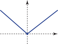
(a)

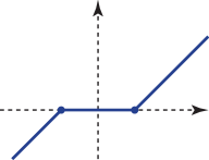
(b)

Figure 1: The dissipation function of Example 3.1 and its proximal operator.

Example 3.1.

As a simple example, consider a truss consisting of $m$ bars. For truss element $l$ $(l=1,\dots,m)$, we use $\sigma_{l}$ and $\Delta\varepsilon_{\mathrm{p}l}$ to denote the axial stress and the incremental axial plastic strain, respectively. The set of admissible stress is given as

$$Y_{l}=\{\sigma_{l}\in\mathbb{R}\mid|\sigma_{l}|\leq R_{l}\},$$

where $R_{l}$ is the magnitude of the yield stress. Then the dissipation function is

$$\delta_{Y_{l}}^{*}(\Delta\varepsilon_{\mathrm{p}l})=R_{l}|\Delta\varepsilon_{\mathrm{p}l}|,$$

which is depicted in Figure 1a. The proximal operator of $\beta_{l}\delta_{Y_{l}}^{*}$, used in line 7 of Algorithm 1, is

$$\mathop{\boldsymbol{\mathsf{prox}}}\nolimits_{\beta_{l}\delta_{Y_{l}}^{*}}(\Delta\varepsilon_{\mathrm{p}l})=\begin{dcases*}\Delta\varepsilon_{\mathrm{p}l}+\beta_{l}R_{l}&if $\Delta\varepsilon_{\mathrm{p}l}<-\beta_{l}R_{l}$,\\ 0&if $|\Delta\varepsilon_{\mathrm{p}l}|\leq\beta_{l}R_{l}$,\\ \Delta\varepsilon_{l}-\beta_{l}R_{l}&if $\Delta\varepsilon_{\mathrm{p}l}>\beta_{l}R_{l}$,\\ \end{dcases*}$$

which is depicted in Figure 1b; see [15] for details. $\blacksquare$

Each iteration of Algorithm 1 consists of the following procedures. In line 3, according to the compatibility relations, we update the incremental elastic strains, by using the incumbent incremental displacement and the incumbent incremental plastic strains. In line 4, we update the stress tensors according to the constitutive equations. In line 5, we compute the unbalanced nodal force vector, $\boldsymbol{r}^{(k)}$, according to the force-balance equation. Line 6 updates the incremental displacement vector, by adding $-\alpha\boldsymbol{r}^{(k)}$ to the incumbent solution, $\Delta\boldsymbol{u}^{(k)}$. This update rule is analogous to the steepest descent method applied to an elastic problem [9]; see (1). Line 7 updates the incremental plastic strains, where the proximal operator of the dissipation function (scaled by $\beta_{l}$) is used. This step is further discussed in section 4.

The computations of Algorithm 1, except for the one in line 7, consist of additions and multiplications, which are computationally very cheap; it is worth noting that $B_{l}$ $(l=1,\dots,m)$ is usually sparse. For the computation in line 7, explicit formulae have been given for the truss [15], von Mises [32], and Tresca [33] yield criteria. Therefore, for these yield criteria, the computation in line 7 is also cheap. Thus, to extend this algorithm to another yield criterion, it is crucial to develop an efficient computational manner for line 7.

It is worth noting that, in practice, we incorporate the acceleration scheme [2] and its restart scheme [28] into Algorithm 1, to reduce the number of iterations required before convergence; see [15, 32, 33]. Also, every step of Algorithm 1 is highly parallelizable. Namely, the computations in lines 3, 4, and 7 are carried out independently for each numerical integration point, and the vector additions in lines 5 and 6 can be performed independently for each row.

4 Understanding as fixed-point iteration

This section provides an interpretation of Algorithm 1 from a perspective of a fixed-point iteration. A key is the following property of the proximal operator.

Lemma 4.1.

Let $f:\mathcal{S}^{3}\to\mathbb{R}\cup\{+\infty\}$ be a closed proper convex function, and $\gamma>0$. For $\boldsymbol{\chi}$, $\boldsymbol{\zeta}\in\mathcal{S}^{3}$, we have $\boldsymbol{\zeta}=\mathop{\boldsymbol{\mathsf{prox}}}\nolimits_{\gamma f}(\boldsymbol{\chi})$ if and only if $\boldsymbol{\chi}=\boldsymbol{\zeta}+\gamma\partial f(\boldsymbol{\zeta})$.

Proof.

See [29, section 3.2]. ∎

In accordance with lines 3 and 4 of Algorithm 1, we write

$$\boldsymbol{\sigma}_{l}(\Delta\boldsymbol{\varepsilon}_{\mathrm{p}l},\Delta\boldsymbol{u})=\boldsymbol{\sigma}_{0l}+\boldsymbol{\mathsf{C}}_{l}(B_{l}\Delta\boldsymbol{u}-\Delta\boldsymbol{\varepsilon}_{\mathrm{p}l}),\quad l=1,\dots,m$$

for notational simplicity, where $\boldsymbol{\sigma}_{l}(\Delta\boldsymbol{\varepsilon}_{\mathrm{p}l},\Delta\boldsymbol{u})$ is the incumbent stress determined from $\Delta\boldsymbol{\varepsilon}_{\mathrm{p}l}$ and $\Delta\boldsymbol{u}$. It follows from (3) that the unbalanced nodal force vector (i.e., the residual of the force-balance equation) can be written as

$$\boldsymbol{r}(\Delta\boldsymbol{u},\Delta\boldsymbol{\varepsilon}_{\mathrm{p}1},\dots,\Delta\boldsymbol{\varepsilon}_{\mathrm{p}m})=\sum_{l=1}^{m}\rho_{l}B_{l}^{*}\boldsymbol{\sigma}_{l}(\Delta\boldsymbol{\varepsilon}_{\mathrm{p}l},\Delta\boldsymbol{u})-\boldsymbol{q}.$$

Then the system of (2), (3), (4), and (6) is equivalently rewritten as

$$\boldsymbol{r}(\Delta\boldsymbol{u},\Delta\boldsymbol{\varepsilon}_{\mathrm{p}1},\dots,\Delta\boldsymbol{\varepsilon}_{\mathrm{p}m}) =\boldsymbol{0},$$ (8)

$$\partial\delta_{Y_{l}}^{*}(\Delta\boldsymbol{\varepsilon}_{\mathrm{p}l})-\boldsymbol{\sigma}_{l}(\Delta\boldsymbol{\varepsilon}_{\mathrm{p}l},\Delta\boldsymbol{u}) \ni\boldsymbol{o},\quad l=1,\dots,m.$$ (9)

We easily see that, for any $\alpha>0$ and $\beta_{l}>0$ $(l=1,\dots,m)$, (8) and (9) are satisfied if and only if

$$\Delta\boldsymbol{u} =\Delta\boldsymbol{u}-\alpha\boldsymbol{r}(\Delta\boldsymbol{u},\Delta\boldsymbol{\varepsilon}_{\mathrm{p}1},\dots,\Delta\boldsymbol{\varepsilon}_{\mathrm{p}m}),$$ (10)

$$\Delta\boldsymbol{\varepsilon}_{\mathrm{p}l} \in\Delta\boldsymbol{\varepsilon}_{\mathrm{p}l}-\beta_{l}(\partial\delta_{Y_{l}}^{*}(\Delta\boldsymbol{\varepsilon}_{\mathrm{p}l})-\boldsymbol{\sigma}_{l}(\Delta\boldsymbol{\varepsilon}_{\mathrm{p}l},\Delta\boldsymbol{u})),$$

$$\qquad\qquad\qquad\qquad l=1,\dots,m$$ (11)

hold. That is, the solution of the elastoplastic incremental problem is characterized as a fixed point of the mappings on the right sides of (10) and (11).

A natural fixed-point iteration applied to (10) is

$$\Delta\boldsymbol{u}^{(k+1)}:=\Delta\boldsymbol{u}^{(k)}-\alpha\boldsymbol{r}(\Delta\boldsymbol{u}^{(k)},\Delta\boldsymbol{\varepsilon}_{\mathrm{p}1}^{(k)},\dots,\Delta\boldsymbol{\varepsilon}_{\mathrm{p}m}^{(k)}).$$

This is exactly same as the computations in lines 3, 4, 5, and 6 of Algorithm 1.

In contrast, we apply a slightly different scheme to (11). Namely, for each $l=1,\dots,m$ we rewrite (11) equivalently as

$$\Delta\boldsymbol{\varepsilon}_{\mathrm{p}l}+\beta_{l}\partial\delta_{Y_{l}}^{*}(\Delta{\boldsymbol{\varepsilon}}_{\mathrm{p}l})\ni\Delta\boldsymbol{\varepsilon}_{\mathrm{p}l}+\beta_{l}\boldsymbol{\sigma}_{l}(\Delta\boldsymbol{\varepsilon}_{\mathrm{p}l},\Delta\boldsymbol{u}),$$ (12)

from which we obtain an iteration

$$\Delta\boldsymbol{\varepsilon}_{\mathrm{p}l}^{(k+1)}+\beta_{l}\partial\delta_{Y_{l}}^{*}(\Delta{\boldsymbol{\varepsilon}}_{\mathrm{p}l}^{(k+1)})\ni\Delta\boldsymbol{\varepsilon}_{\mathrm{p}l}^{(k)}+\beta_{l}\boldsymbol{\sigma}_{l}(\Delta\boldsymbol{\varepsilon}_{\mathrm{p}l}^{(k)},\Delta\boldsymbol{u}^{(k)}).$$ (13)

It follows from Lemma 4.1 that (13) is equivalent to

$$\Delta\boldsymbol{\varepsilon}_{\mathrm{p}l}^{(k+1)}=\mathop{\boldsymbol{\mathsf{prox}}}\nolimits_{\beta_{l}\delta_{Y_{l}}^{*}}(\Delta\boldsymbol{\varepsilon}_{\mathrm{p}l}^{(k)}+\beta_{l}\boldsymbol{\sigma}_{l}(\Delta\boldsymbol{\varepsilon}_{\mathrm{p}l}^{(k)},\Delta\boldsymbol{u}^{(k)})).$$ (14)

This corresponds to line 7 of Algorithm 1. Since application of the proximal operator of a closed proper convex function to any point always results in a (nonempty) unique point [29, section 1.1], the right side of (14) is guaranteed to be uniquely determined.

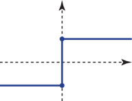
Figure 2: The associated flow rule of Example 3.1.

Remark 4.1.

We have seen that the update rule of the plastic strain, (14), of Algorithm 1 can be obtained not from (11) but from (12). If we adopt (11), application of a fixed-point iteration yields

$$\Delta\boldsymbol{\varepsilon}_{\mathrm{p}l}^{(k+1)}\in\Delta\boldsymbol{\varepsilon}_{\mathrm{p}l}^{(k)}-\beta_{l}(\partial\delta_{Y_{l}}^{*}(\Delta\boldsymbol{\varepsilon}_{\mathrm{p}l}^{(k)})-\boldsymbol{\sigma}_{l}(\Delta\boldsymbol{\varepsilon}_{\mathrm{p}l}^{(k)},\Delta\boldsymbol{u}^{(k)})).$$ (15)

However, this is not adequate as an update rule, because $\partial\delta_{Y_{l}}^{*}(\Delta\boldsymbol{\varepsilon}_{\mathrm{p}l}^{(k)})$ on the right side of (15) is, in general, not determined uniquely. For example, in the truss case considered in Example 3.1, Figure 2 shows $\partial\delta_{Y_{l}}^{*}(\Delta\varepsilon_{\mathrm{p}l})$, where $\delta_{Y_{l}}^{*}(\Delta\varepsilon_{\mathrm{p}l})$ is shown in Figure 1a. It is observed in Figure 2 that $\partial\delta_{Y_{l}}^{*}(\Delta\varepsilon_{\mathrm{p}l})$ is not unique at $\Delta\varepsilon_{\mathrm{p}l}=0$. In contrast, as mentioned above, $\Delta\boldsymbol{\varepsilon}_{\mathrm{p}l}^{(k+1)}$ satisfying (13) exists uniquely, which makes Algorithm 1 well-defined. $\blacksquare$

Remark 4.2.

To provide another viewpoint, observe that (13) is equivalently written as

$$\boldsymbol{\sigma}_{l}(\Delta\boldsymbol{\varepsilon}_{\mathrm{p}l}^{(k)},\Delta\boldsymbol{u}^{(k)})-\frac{1}{\beta_{l}}(\Delta\boldsymbol{\varepsilon}_{\mathrm{p}l}^{(k+1)}-\Delta\boldsymbol{\varepsilon}_{\mathrm{p}l}^{(k)})\in\partial\delta_{Y_{l}}^{*}(\Delta\boldsymbol{\varepsilon}_{\mathrm{p}l}^{(k+1)}).$$ (16)

This is analogous to the associated flow rule in (6), but the second term on the left side seems to be additional. One may consider that a natural update rule based on (6) is

$$\boldsymbol{\sigma}_{l}(\Delta\boldsymbol{\varepsilon}_{\mathrm{p}l}^{(k)},\Delta\boldsymbol{u}^{(k)})\in\partial\delta_{Y_{l}}^{*}(\Delta\boldsymbol{\varepsilon}_{\mathrm{p}l}^{(k+1)}).$$ (17)

However, (17) is not adequate, because for $\boldsymbol{\sigma}_{l}(\Delta\boldsymbol{\varepsilon}_{\mathrm{p}l}^{(k)},\Delta\boldsymbol{u}^{(k)})\not\in Y_{l}$ there exists no $\Delta\boldsymbol{\varepsilon}_{\mathrm{p}l}^{(k+1)}$ satisfying (17); see Figure 2 for the truss case. In contrast, as mentioned above, for any $\boldsymbol{\sigma}_{l}(\Delta\boldsymbol{\varepsilon}_{\mathrm{p}l}^{(k)},\Delta\boldsymbol{u}^{(k)})$ and $\Delta\boldsymbol{\varepsilon}_{\mathrm{p}l}^{(k)}$, $\Delta\boldsymbol{\varepsilon}_{\mathrm{p}l}^{(k+1)}$ satisfying (16) exists uniquely. $\blacksquare$

5 Conclusions

This short paper has presented a unified form of proximal gradient method to solve quasi-static incremental problems in elastoplastic analysis of structures. An interpretation of the presented algorithm has also been provided from a viewpoint of mechanics. Although in this paper we have restricted ourselves to perfect plasticity, extension of the presented results to problems with strain hardening is possible; one can refer to [15, 32, 33] for cases with specific yield criteria.

The presented general form of the algorithm, as well as interpretation, sheds new light on numerical methods in computational plasticity. For example, although this paper has been restricted to quasi-static incremental problems, it can possibly provide us with a guide for development of similar algorithms solving other problems in plasticity, including, e.g., limit analysis and shakedown analysis. Such algorithms combined with an acceleration scheme may possibly be efficient compared with conventional methods in plasticity, because it has been reported for quasi-static incremental problems that accelerated proximal gradient methods outperform conventional optimization-based approaches, especially for large-scale problems [15, 32, 33].

Acknowledgments

The work described in this paper is partially supported by JSPS KAKENHI 17K06633 and JST CREST Grant Number JPMJCR1911, Japan.

References

- Anjos and Lasserre [2012] M. F. Anjos, J. B. Lasserre (eds.): Handbook on Semidefinite, Conic and Polynomial Optimization. Springer, New York (2012).
- Beck and Teboulle [2009] A. Beck, M. Teboulle: A fast iterative shrinkage-thresholding algorithm for linear inverse problems. SIAM Journal on Imaging Sciences, 2, 183–202 (2009).
- Bisbos [2007] C. D. Bisbos: Semidefinite optimization models for limit and shakedown analysis problems involving matrix spreads. Optimization Letters, 1, 101–109 (2007).
- Bisbos et al. [2005] C. D. Bisbos, A. Makrodimopoulos, P. M. Pardalos: Second-order cone programming approaches to static shakedown analysis in steel plasticity. Optimization Methods and Software, 20, 25–52 (2005).
- Bisbos and Pardalos [2007] C. D. Bisbos, P. M. Pardalos: Second-order cone and semidefinite representations of material failure criteria. Journal of Optimization Theory and Applications, 134, 275–301 (2007).
- Chambolle and Pock [2011] A. Chambolle, T. Pock: A first-order primal-dual algorithm for convex problems with applications to imaging. Journal of Mathematical Imaging and Vision, 40, 120–145 (2011).
- Combettes and Wajs [2005] P. L. Combettes, V. R. Wajs: Signal recovery by proximal forward-backward splitting. Multiscale Modeling and Simulation, 4, 1168–1200 (2005).
- Daubechies et al. [2004] I. Daubechies, M. Defrise, C. De Mol: An iterative thresholding algorithm for linear inverse problems with a sparsity constraint. Communications on Pure and Applied Mathematics, 57, 1413–1457 (2004).
- Fujita and Kanno [2019] S. Fujita, Y. Kanno: Application of accelerated gradient method to equilibrium analysis of trusses with nonlinear elastic materials (in Japanese). Journal of Structural and Construction Engineering (Transactions of AIJ), 84, 1223–1230 (2019).
- Goldstein et al. [2014] T. Goldstein, B. O’Donoghue, S. Setzer, R. Baraniuk: Fast alternating direction optimization methods. SIAM Journal on Imaging Science, 7, 1588–1623 (2014).
- Gueguin et al. [2014] M. Gueguin, G. Hassen, P. de Buhan: Numerical assessment of the macroscopic strength criterion of reinforced soils using semidefinite programming. International Journal for Numerical Methods in Engineering, 99, 522–541 (2014).
- Han and Reddy [2013] W. Han, B. D. Reddy: Plasticity (2nd ed.). Springer, New York (2013).
- Ito et al. [2017] N. Ito, A. Takeda, K.-C. Toh: A unified formulation and fast accelerated proximal gradient method for classification. Journal of Machine Learning Research, 18, 1–49 (2017).
- Kanno [2011] Y. Kanno: Nonsmooth Mechanics and Convex Optimization. CRC Press, Boca Raton (2011).
- Kanno [2016] Y. Kanno: A fast first-order optimization approach to elastoplastic analysis of skeletal structures. Optimization and Engineering, 17, 861–896 (2016).
- Krabbenhøft and Lyamin [2012] K. Krabbenhøft, A. V. Lyamin: Computational Cam clay plasticity using second-order cone programming. Computer Methods in Applied Mechanics and Engineering, 209–212, 239–249 (2012).
- Krabbenhøft et al. [2007] K. Krabbenhøft, A. V. Lyamin, S. W. Sloan: Formulation and solution of some plasticity problems as conic programs. International Journal of Solids and Structures, 44, 1533–1549 (2007).
- Krabbenhøft et al. [2008] K. Krabbenhøft, A. V. Lyamin, S. W. Sloan: Three-dimensional Mohr–Coulomb limit analysis using semidefinite programming. Communications in Numerical Methods in Engineering, 24, 1107–1119 (2008).
- Lee and Sidford [2013] Y. T. Lee, A. Sidford: Efficient accelerated coordinate descent methods and faster algorithms for solving linear systems. Proceedings of the 2013 IEEE 54th Annual Symposium on Foundations of Computer Science (FOCS ’13), 147–156 (2013).
- Makrodimopoulos [2006] A. Makrodimopoulos: Computational formulation of shakedown analysis as a conic quadratic optimization problem. Mechanics Research Communications, 33, 72–83 (2006).
- Makrodimopoulos [2010] A. Makrodimopoulos: Remarks on some properties of conic yield restrictions in limit analysis. International Journal for Numerical Methods in Biomedical Engineering, 26, 1449–1461 (2010).
- Makrodimopoulos and Martin [2006] A. Makrodimopoulos, C. M. Martin: Lower bound limit analysis of cohesive-frictional materials using second-order cone programming. International Journal for Numerical Methods in Engineering, 66, 604–634 (2006).
- Makrodimopoulos and Martin [2007] A. Makrodimopoulos, C. M. Martin: Upper bound limit analysis using simplex strain elements and second-order cone programming. International Journal for Numerical and Analytical Methods in Geomechanics, 31, 835–865 (2007).
- Martin and Makrodimopoulos [2008] C. M. Martin, A. Makrodimopoulovs: Finite-element limit analysis of Mohr–Coulomb materials in 3D using semidefinite programming. Journal of Engineering Mechanics (ASCE), 134, 339–347 (2008).
- Nesterov [1983] Y. Nesterov: A method of solving a convex programming problem with convergence rate . Soviet Mathematics Doklady, 27, 372–376 (1983).
- Nesterov [2004] Y. Nesterov: Introductory Lectures on Convex Optimization: A Basic Course. Kluwer Academic Publishers, Dordrecht (2004).
- Nocedal and Wright [2006] J. Nocedal, S. J. Wright: Numerical Optimization (2nd ed.). Springer, New York (2006).
- O’Donoghue and Candès [2015] B. O’Donoghue, E. Candès: Adaptive restart for accelerated gradient schemes. Foundations of Computational Mathematics, 15, 715–732 (2015).
- Parikh and Boyd [2014] N. Parikh, S. Boyd: Proximal algorithms. Foundations and Trends in Optimization, 1, 127–239 (2014).
- Rockafellar [1970] R. T. Rockafellar: Convex Analysis. Princeton University Press, Princeton (1970).
- Scalet and Auricchio [2018] G. Scalet, F. Auricchio: Computational methods for elastoplasticity: an overview of conventional and less-conventional approaches. Archives of Computational Methods in Engineering, 25, 545–589 (2018)
- Shimizu and Kanno [2018] W. Shimizu, Y. Kanno: Accelerated proximal gradient method for elastoplastic analysis with von Mises yield criterion. Japan Journal of Industrial and Applied Mathematics, 35, 1–32 (2018).
- Shimizu and Kanno [2020] W. Shimizu, Y. Kanno: A note on accelerated proximal gradient method for elastoplastic analysis with Tresca yield criterion. Journal of the Operations Research Society of Japan, to appear.
- Toh and Yun [2010] K.-C. Toh, S. Yun: An accelerated proximal gradient algorithm for nuclear norm regularized linear least squares problems. Pacific Journal of Optimization, 6, 615–640 (2010).
- Yamaguchi and Kanno [2016] T. Yamaguchi, Y. Kanno: Ellipsoidal load-domain shakedown analysis with von Mises yield criterion: a robust optimization approach. International Journal for Numerical Methods in Engineering, 107, 1136–1144 (2016).
- Yonekura and Kanno [2012] K. Yonekura, Y. Kanno: Second-order cone programming with warm start for elastoplastic analysis with von Mises yield criterion. Optimization and Engineering, 13, 181–218 (2012).