Can Two Forecasts Have the Same Conditional Expected Accuracy?

Abstract

The approach for testing equal predictive accuracy for pairs of forecasting models proposed by Giacomini and White, (2006) assumes that the parameters of the underlying forecasting models are estimated using a rolling window of fixed width and incorporates the effect of parameter estimation in the null hypothesis. We show that a necessary and sufficient condition for the conditionally expected loss differential of two forecasting models to be a martingale difference sequence is that the outcome is a simple average of the two forecasts. When the forecasts contain parameter estimation errors, this means that the conditional mean of the outcome has to be a function of past estimation errors–a condition that fails in many situations. We also show that the null can fail even in the absence of parameter estimation for many types of stochastic processes in common use.

1 Introduction

In an important contribution to the literature on economic forecasting, Giacomini and White, (2006) (GW, henceforth) develop a novel approach for comparing the accuracy of alternative economic forecasts and test the null of equal expected predictive accuracy. GW incorporate the effect of parameter estimation in the null hypothesis and assume that estimation error does not vanish asymptotically by requiring that fixed-length windows are used to estimate the parameters of the underlying forecasting models. Using this approach, simple tests of equal predictive accuracy do not have a degenerate limiting distribution even in comparisons of nested forecasting models, thus addressing a key problem causing difficulties for earlier tests.

The GW test has found widespread use in applied work in economics and has become the standard method for comparing the predictive accuracy of nested forecasting models while accounting for the effect of parameter estimation. It is, therefore, important to establish conditions under which the null hypothesis entertained by GW is valid and so can be used to compare the predictive accuracy of alternative forecasts. The null hypothesis in GW is that the expected loss differential, i.e., the difference between the expected loss of a pair of forecasts, is a martingale difference sequence (MDS) conditional on some information set which typically includes, at a minimum, current and past observations of the outcome and data used to generate the forecasts.

We show here that the MDS property conditional on past data fails to hold in many situations when the forecasts are generated using a set of estimated model parameters as assumed in the analysis of GW. This conclusion holds regardless of whether a fixed-width rolling window or an expanding window is used to estimate the parameters of the underlying forecasting models and regardless of whether the models are nested or non-nested. Caution should therefore be exercised when applying the conditional GW test to compare the performance of forecasting models. Even in the absence of parameter estimation error, we show that the MDS property fails whenever the underlying data generating process (DGP) for the outcome does not satisfy a restrictive finite dependence condition that rules out many standard models used in applied work.

This conclusion has important practical implications. In particular, there can be substantial autocorrelation in the loss difference and we show that the GW test can result in severe size distortions for testing an unconditional null using popular schemes for estimating the long-run variance of the loss differential. We also establish a valid procedure for testing that the null of equal predictive accuracy of two rolling-window forecasts holds “on average”. This sub-sampling t-test approach uses a self-normalization structure and avoids directly constructing robust standard errors that account for serial correlation in the loss differentials.

It is worth emphasizing that our analysis pertains to tests of the null hypothesis that the expected loss differential is mean-zero conditional on the parameter estimates used by the underlying forecasting models and possibly other information. It does not apply to tests of the null that the unconditional mean of the loss differential equals zero. This unconditional null does not require that two forecasts are equally accurate at each point in time but only that they are equally accurate on average. Testing this unconditional null is more common in practice and is typically conducted using the popular Diebold-Mariano test.

The outline of our analysis is as follows. Section 2 introduces our setup and demonstrates that the GW null fails to be valid in the presence of estimated parameters and also fails in the absence of a restrictive finite dependence condition on the DGP. Second 3 pursues practical implications of our theoretical results, while Second 4 analyzes tests of the null that the forecasts have the same unconditionally expected loss, and Section 5 concludes. Proofs are contained in an appendix.

2 The null of equal conditional expected predictive accuracy

This section introduces the forecast environment and demonstrates that the GW null is not, in general, appropriate for comparing the conditionally expected loss of a pair of forecasting models.

2.1 Setup

Our forecast environment closely mirrors the setup in GW. We are interested in comparing the predictive accuracy of a pair of one-step-ahead forecasts $f_{1,t},f_{2,t}$ of some variable $Y_{t+1}$. Each forecast is generated using information available at time $t\mbox{,}$ $\mathcal{F}_{t}=\sigma(W_{1}^{\prime},W_{2}^{\prime},...,W_{t}^{\prime})$, where $W_{t}=(Y_{t},X_{t}^{\prime})^{\prime}$, and $X_{t}$ is a set of predictor variables. Hence, $\mathcal{F}_{t}$ contains current and past values of the outcome, forecast and predictors. GW carefully state that the forecasts are adapted to the most recent $m$ values of $W_{t}$, i.e., $f_{i,t}=f(W_{t},W_{t-1},...,W_{t-m+1};\hat{\beta}_{i,t,m})$. The setup includes, but is not limited to, linear prediction models of the form $y_{t+1}=\beta_{i}^{\prime}X_{it}+\varepsilon_{it+1},$estimated by least squares, i.e., $\hat{\beta}_{i,t,m}=\left(\sum_{s=t-m}^{t-1}X_{is}X_{is}^{\prime}\right)^{-1}\left(\sum_{s=t-m}^{t-1}X_{is}y_{s+1}\right)$.

The precision of the forecasts is evaluated using a loss function, $L(y_{t+1},f_{i,t})$ which is a mapping from the space of outcomes and forecasts to the real line. Under the commonly used squared error loss, $L(y_{t+1},f_{i,t})=e_{i,t+1}^{2}$, where $e_{i,t+1}=y_{t+1}-f_{i,t}$ ($i=1,2$) is the forecast error. Furthermore, following Diebold and Mariano, (1995), define the loss differential as the loss of model 1 relative to that of model 2:

$$\Delta L_{t+1}\equiv\Delta L_{t+1}(y_{t+1},f_{1,t},f_{2t})=L(y_{t+1},f_{1,t})-L(y_{t+1},f_{2,t,m}).$$ (1)

Under squared error loss,

$$\Delta L_{t+1}=(y_{t+1}-f_{1,t})^{2}-(y_{t+1}-f_{2,t})^{2}.$$ (2)

The null hypothesis considered by GW is that, conditional on some information set, $\mathcal{G}_{t}$, the loss differential is a martingale difference sequence (MDS):

$$E[\Delta L_{t+1}(y_{t+1},f_{1,t},f_{2t})|\mathcal{G}_{t}]=0,$$ (3)

almost surely for $t=1,2,...$. GW write that “Note that we do not require $\mathcal{G}_{t}=\mathcal{F}_{t}$, although this is a leading case of interest…” For simplicity, in the rest of the paper, we focus on this leading case with $\mathcal{G}_{t}=\mathcal{F}_{t}$.

Forecast comparisons are often conducted using (pseudo) out-of-sample evaluation methods which split a sample of $T$ observations into an initial sample using $m$ observations for parameter estimation and a forecast evaluation sample which consists of the remaining $n$ observations, so $T=n+m$. GW assume that $m$ is bounded by a finite constant although, in general, we can regard $m=m_{T}$ and $n=n_{T}$ as functions of $T$. For notational simplicity, we suppress the subscripts.

To test the null in (3), GW propose the test statistic

$$GW_{T}=\frac{\sum_{t=m}^{T-1}\Delta L_{t+1}}{\sqrt{\sum_{t=m}^{T-1}(\Delta L_{t+1})^{2}}}.$$ (4)

The simple expression in the denominator exploits the property that, under the null (3) that $\Delta L_{t+1}$ follows a MDS, there is no need to correct for possible serial correlation in $\Delta L_{t+1}$.

To test the hypothesis that $E[\Delta L_{t+1}\mid\mathcal{F}_{t}]=0$ almost surely, GW point out that one can choose any random variable $h_{t}\in\mathcal{F}_{t}$ and test the unconditional moment condition $E(\Delta L_{t+1}h_{t})=0$. However, when $P(E[\Delta L_{t+1}\mid\mathcal{F}_{t}]=0)<1$, there exists a variable $h_{t}^{*}\in\mathcal{F}_{t}$ such that $E(\Delta L_{t+1}h_{t}^{*})\neq 0$. Hence, results in GW hinge on the MDS condition which we examine in this paper.

2.2 Implications of the MDS null

We first establish a necessary and sufficient condition for the validity of the null hypothesis in (3):

Proposition 1.

Assume that $f_{1,t}\neq f_{2,t}$ almost surely. Then under squared error loss $E(\Delta L_{t+1}\mid\mathcal{F}_{t})=0$ almost surely if and only if $E(y_{t+1}\mid\mathcal{F}_{t})=(f_{1,t}+f_{2,t})/2$ almost surely.

This result shows that the conditionally expected loss differential follows an MDS process if and only if the conditional expectation of the outcome is a simple average of the two forecasts. When the forecasts contain parameter estimation errors, this means that the conditional mean of $y_{t+1}$ has to be a function of past estimation errors. This is quite unnatural as DGPs are typically considered to be objective processes whose dynamics is not related to an estimation scheme.

Proposition 1 can be used constructively to establish cases in which the null hypothesis in (3) is valid, as we next show.

Example 1.

Suppose that $y_{t+1}=\rho y_{t}+\varepsilon_{t+1}$ with $E[\varepsilon_{t+1}|\mathcal{F}_{t}]$=0, so $E[y_{t+1}\mid\mathcal{F}_{t}]=\rho y_{t}$. Moreover, if $f_{1,t}=(\rho-\delta)y_{t}$ and $f_{2,t}=(\rho+\delta)y_{t}$, then $E[y_{t+1}|\mathcal{F}_{t}]=\frac{1}{2}(f_{1,t}+f_{2,t})$ so that, from Proposition 1, the squared error loss differential follows an MDS process.

A popular practice is to estimate the parameters of the forecasting model using the most recent $m$ observations. In our leading case as well as in GW, $m$ is fixed or bounded, so that estimation errors do not vanish, while the asymptotic analysis lets $n\rightarrow\infty$. As we shall see, this case can never satisfy $E(y_{t+1}\mid\mathcal{F}_{t})=(f_{1,t}+f_{2,t})/2$ almost surely without a restrictive finite dependence condition and so the MDS condition (3) cannot hold.

Example 2.

As a simple example with estimation error, let $\bar{x}_{i,t}=m^{-1}\sum_{s=0}^{m-1}x_{i,t-m}$ for $i=1,2$ be $m$-period moving averages, while

$$y_{t+1}=\frac{1}{2}\bar{x}_{1,t}+\frac{1}{2}\bar{x}_{2,t}+\varepsilon_{t+1},$$

where $\varepsilon_{t+1}$ is an MDS so $E[\varepsilon_{t+1}|\mathcal{F}_{t}]=0$. Setting $f_{1,t}=\bar{x}_{1,t}$ and $f_{2,t}=\bar{x}_{2,t}$, both forecasts use misspecified (under-dimensioned) forecasting models that omit one moving average component. However, once again we have $E[y_{t+1}|\mathcal{F}_{t}]=\frac{1}{2}\bar{x}_{1,t}+\frac{1}{2}\bar{x}_{2,t}=\frac{1}{2}(f_{1,t}+f_{2,t})$, so it follows from Proposition 1 that the squared error loss follows an MDS process.

Even for forecasts that do not depend on estimated parameters, we can show that the MDS property fails whenever the underlying DGP does not satisfy the restrictive finite dependence condition. In particular, let $\mathcal{F}_{t-m:t}$ denote the $\sigma$-algebra generated by data from time $t-m$ to $t$. All forecasts based on a rolling window of size $m$ are $\mathcal{F}_{t-m:t}$-measurable; this allows for any estimation methodology ranging from the basic least-squares estimators to sophisticated machine learning methods. Recall that $\mathcal{F}_{t}$ denotes the $\sigma$-algebra generated by all the data up to time $t$.

We next show that the MDS condition (3) cannot hold for $\Delta L_{t+1}$ if the outcome variable $y_{t+1}$ does not have finite dependence:

Proposition 2.

Assume that $f_{1,t}\neq f_{2,t}$ almost surely and $P\left(E(y_{t+1}\mid\mathcal{F}_{t})=E(y_{t+1}\mid\mathcal{F}_{t-m:t})\right)<1$. If $f_{1,t}$ and $f_{2,t}$ are both $\mathcal{F}_{t-m,t}$-measurable, then $\{\Delta L_{t+1},\mathcal{F}_{t}\}$ is not a martingale difference sequence, i.e., $P(E(\Delta L_{t+1}\mid\mathcal{F}_{t})=0)<1$.

The finite-dependence condition in Proposition 2 requires that the conditional mean of $y_{t+1}$ only depends on the most recent $m$ data points. This condition is ruled out by many widely used models that are not finite-order Markov such as MA and ARMA processes as well as unobserved components (state space) models and GARCH-in-mean processes.

2.3 MDS Property and Estimation Scheme

Proposition 2 shows that unless $E(y_{t+1}\mid\mathcal{F}_{t})=E(y_{t+1}\mid\mathcal{F}_{t-m:t})$ with probability one, the loss difference cannot be an MDS, no matter how one computes the forecasts with or without estimated parameters and regardless of the estimation method. The result also does not require us to make specific assumptions on the DGP such as stationarity. Hence, in the absence of the restrictive finite dependence condition, there is an inherent contradiction between the MDS property and rolling window estimation.

In most forecasting problems, the main challenge is to model and estimate the conditional mean $E(y_{t+1}\mid\mathcal{F}_{t})$. However, Proposition 1 says that the MDS null is equivalent to $E(y_{t+1}\mid\mathcal{F}_{t})=(f_{1,t}+f_{2,t})/2$. Since $f_{1,t}$ and $f_{2,t}$ are computed from a fixed-width rolling window, this result is saying that the true conditional mean $E(y_{t+1}\mid\mathcal{F}_{t})$ can be learned from the data without letting the sample size increase.

This is quite a restrictive setup. Even if we have a correctly specified parametric model $f(W_{1:t};\theta)$ for the entire distribution $y_{t+1}\mid\mathcal{F}_{t}$ with parameter $\theta$, the optimal estimator (i.e., the maximum likelihood estimate) for $\theta$ in the rolling window of length $R$ would have an error of rate $O(R^{-1/2})$. Hence, having no estimation error at all for $E(y_{t+1}\mid\mathcal{F}_{t})$ for fixed $R$ is hard to imagine.

In the following AR$(q)$ example, we show that the MDS null fails to hold under realistic estimation schemes with finite estimation windows.

Example 3.

$Y_{t+1}=\sum_{j=1}^{q}\rho_{j}Y_{t+1-j}+\varepsilon_{t+1}$, where $\varepsilon_{t+1}$ is i.i.d with $E(\varepsilon_{t+1})=0$. Thus, the $\sigma$-algebra from the observed data is $\mathcal{F}_{t}=\sigma(Y_{t},Y_{t-1},...)$. Suppose that $f_{1,t}=X_{t,1}^{\prime}\hat{\beta}_{t,1}$ and $f_{2,t}=X_{t,2}^{\prime}\hat{\beta}_{t,2}$, where $X_{t,1}\in\mathbb{R}^{q_{1}}$ and $X_{t,2}\in\mathbb{R}^{q_{2}}$ with $\max\{q_{1},q_{2}\}\leq q$ are vectors with elements in $Y_{t-q:t}:=(Y_{t},...Y_{t-q})^{\prime}$. For $j\in\{1,2\}$, we assume that $\hat{\beta}_{t,j}=g_{j}(Y_{t},Y_{t-1},...,Y_{t-m_{j}})$ for some measurable function $g_{j}$, where $m_{j}>q_{j}$ is finite. Notice that some components of $\hat{\beta}_{t,j}$ are allowed to be zero; hence, without loss of generality, we can assume that $X_{t,1}=X_{t,2}=Y_{t-q:t}$.

Building on this example, we have the following result:

Lemma 1.

Suppose that $Y_{t+1}=\sum_{j=1}^{q}\rho_{j}Y_{t+1-j}+\varepsilon_{t+1}$, where $\varepsilon_{t+1}$ is i.i.d with $E(\varepsilon_{t+1})=0$. Assume that $f_{1,t}\neq f_{2,t}$ almost surely and that $\varepsilon_{t+1}$ has a density. If $P\left({\rm Var}(\hat{\beta}_{t,1}+\hat{\beta}_{t,2}\mid Y_{t-q:t})>0\right)>0$, then $\{\Delta L_{t+1},\mathcal{F}_{t}\}$ is not a martingale difference sequence.

The requirement that $P\left({\rm Var}(\hat{\beta}_{t,1}+\hat{\beta}_{t,2}\mid Y_{t-q:t})>0\right)>0$ almost surely is very weak and only rules out cases in which ${\rm Var}(\hat{\beta}_{t,1}+\hat{\beta}_{t,2}\mid Y_{t-q:t})$ is never positive, for sure. Typically, the estimation window is larger than the number of lags $q$. Therefore, we should expect that entries $Y_{s}$ for $s<t-q$ will affect $\hat{\beta}_{t,1}+\hat{\beta}_{t,2}$. As a result, conditional on $Y_{t-q:t}$, we should expect non-zero variations in $\hat{\beta}_{t,1}+\hat{\beta}_{t,2}$. By Lemma 1, for autoregressive DGPs with $q$ lags, we should not expect the MDS null to hold if the estimation window is larger than $q$ under commonly used estimators (OLS, MLE or GMM).

2.4 Nested models

For the nested case, consider the DGP

$$y_{t+1}=\beta^{\prime}X_{t}+\varepsilon_{t+1},$$ (5)

where $X_{t}=(1,x_{t})^{\prime}\in\mathbb{R}^{2}$ is a vector of fixed regressors and $\varepsilon_{t+1}$ is i.i.d from $N(0,\sigma^{2})$. Consider the forecasts from a big model (intercept and $x_{t}$) and a small model (intercept only): $f_{1,t}=X_{t}^{\prime}\hat{\beta}_{t,m}$ with $\hat{\beta}_{t,m}=\left(\sum_{s=t-m}^{t-1}X_{s}X_{s}^{\prime}\right)^{-1}\left(\sum_{s=t-m}^{t-1}X_{s}y_{s+1}\right)$ and $f_{2,t}=m^{-1}\sum_{s=t-m}^{t-1}y_{s+1}$.

Proposition 3.

Let $X_{t}=(1,x_{t})^{\prime}\in\mathbb{R}^{2}$, $X_{(t-1)}=(X_{0},\cdots,X_{t-1})^{\prime}\in\mathbb{R}^{t\times 2}$, $x_{(t-1)}=(x_{0},\cdots,x_{t-1})^{\prime}\in\mathbb{R}^{t}$ and $1_{t}=(1,\cdots,1)^{\prime}\in\mathbb{R}^{t}$. Suppose that

$$c^{2}=\sigma^{2}\left[\sum_{t=m+1}^{m+n}\left(X_{t-1}^{\prime}\left(X_{(t-1)}^{\prime}X_{(t-1)}\right)^{-1}X_{t-1}-\frac{x_{t}^{2}}{x_{(t-1)}^{\prime}x_{(t-1)}}\right)\right]/\left[\sum_{t=m+1}^{m+n}\left(1-\frac{x_{(t-1)}^{\prime}1_{t-1}}{x_{(t-1)}^{\prime}x_{(t-1)}}x_{t}\right)^{2}\right].$$ (6)

Then, under squared error loss (2),

1. $E\left[\sum_{t=m+1}^{m+n}\Delta L_{t}\right]=0$.

2. $\{\Delta L_{t+1},\mathcal{F}_{t}\}$ is not a Martingale Difference Sequence, i.e., $P\left[E(\Delta L_{t+1}\mid\mathcal{F}_{t})=0\right]<1$.

Proposition 3 holds for any sample size and has two implications. First, the MDS condition fails when $m$ is fixed (rolling estimation window) and the length of the out-of-sample period ($n$) tends to infinity. Second, the MDS condition also fails when both $m$ and $n$ tend to infinity, i.e., with an expanding estimation window.

2.5 Non-nested models

For the case with non-nested models consider the DGP

$$y_{t+1}=\beta_{1}x_{1t}+\beta_{2}x_{2t}+\varepsilon_{t+1},$$ (7)

where $E(\varepsilon_{t+1}\mid\mathcal{F}_{t})=0$. We use $f_{1,t}=\hat{\beta}_{1t}x_{1t}$ and $f_{2,t}=\hat{\beta}_{2t}x_{2t}$, where $\hat{\beta}_{it}=\left(\sum_{s=t-m}^{t-1}x_{is}^{2}\right)^{-1}\left(\sum_{s=t-m}^{t-1}x_{is}y_{s+1}\right)$ for $i\in\{1,2\}$. The following result states that the MDS condition (3) fails:

Proposition 4.

Consider the DGP in (7) and assume squared error loss (2). Then (1) If $P(\beta_{1}x_{1t}\neq\beta_{2}x_{2t})=1$ and $P(\beta_{1}x_{1t}+\beta_{2}x_{2t}=0)\neq 1$, we do not have $P\left[E(\Delta L_{t+1}\mid\mathcal{F}_{t})=0\right]=1$.
(2) Let $f_{1,t}=\hat{\beta}_{1t}x_{1t}$ and $f_{2,t}=\hat{\beta}_{2t}x_{2t}$ with estimates $\hat{\beta}_{1t}$ and $\hat{\beta}_{2t}$ being $\mathcal{F}_{t}$-measurable. If $P(\hat{\beta}_{1t}x_{1t}\neq\hat{\beta}_{2t}x_{2t})=1$ and $P\left(2(\beta_{1}x_{1t}+\beta_{2}x_{2t})=\hat{\beta}_{1t}x_{1t}+\hat{\beta}_{2t}x_{2t}\right)\neq 1$, then we do not have $P\left[E(\Delta L_{t+1}\mid\mathcal{F}_{t})=0\right]=1$.

Proposition 4 holds regardless of the sample size, $m$, used to estimate the parameters $\hat{\beta}_{it}$, $i=1,2$. This again means that the MDS condition fails when $m$ is fixed and $n$ tends to infinity or when both $m$ and $n$ tend to infinity.

3 Practical Implications

Proposition 1 has some interesting practical implications. To see this, define the forecast error from a simple equal-weighted average of forecasts:

$$\xi_{t+1}=y_{t+1}-(f_{1,t}+f_{2,t})/2.$$ (8)

From Proposition 1, the MDS null hypothesis for the loss differential can equivalently be stated as $E(\xi_{t+1}\mid\mathcal{F}_{t})=0$, motivating a test that is different from the GW test that is based on the loss differential.

A priori, it may not be obvious whether it is better, in a given sample, to test $E(\Delta L_{t+1}\mid\mathcal{F}_{t})=0$ or $E(\xi_{t+1}\mid\mathcal{F}_{t})=0$. Although such tests are equivalent, their finite sample power could well be very different and practitioners will want to maximize power in testing the MDS null. In some situations, an alternative test based on $\xi_{t+1}$ might have better power properties than one based on $\Delta L_{t+1}$.

We next illustrate this point through an analytical example and an empirical application.

3.1 Power for AR(1) Process

Following McCracken, (2020), consider the following first-order autoregressive DGP:

$$y_{t+1}=\rho y_{t}+\varepsilon_{t+1},$$ (9)

where $\varepsilon_{t+1}$ is i.i.d with $E\varepsilon_{t+1}=0$ and $E\varepsilon_{t+1}^{2}=\sigma^{2}$. Assume that $E|\varepsilon_{t+1}|^{3}$ is bounded. Let $f_{1,t}=y_{t}$ and $f_{2,t}=0$ so that $E(\Delta L_{t+1}\mid\mathcal{F}_{t})=0$ when $\rho=1/2$. To examine local power, let $\rho=1/2-T^{-1/2}c$, where $c\in\mathbb{R}$ is a constant and $T$ is the sample sized used for the test. To simplify notations, let $h_{t}=(f_{1,t}+f_{2,t})/2$ and consider the following test statistics:

$$GW_{T}=\frac{T^{-1/2}\sum_{t=1}^{T}\Delta L_{t+1}h_{t}}{\sqrt{T^{-1}\sum_{t=1}^{T}\left(\Delta L_{t+1}h_{t}\right)^{2}}},$$ (10)

and

$$J_{T}=\frac{T^{-1/2}\sum_{t=1}^{T}\xi_{t+1}h_{t}}{\sqrt{T^{-1}\sum_{t=1}^{T}\left(\xi_{t+1}h_{t}\right)^{2}}}.$$ (11)

Both test statistics use critical values from a standard Gaussian distribution, $\Phi$. For a test of nominal size $\alpha$, we therefore reject the null if $|GW_{T}|>cv_{\alpha}\equiv\Phi^{-1}(1-\alpha/2)$ and $|J_{T}|>cv_{\alpha}$ under the GW and $J$ tests, respectively. The following result can be used to compute the power of the tests.

Proposition 5.

Suppose $y_{t+1}$ is generated from a first-order autoregressive process $y_{t+1}=\rho y_{t}+\varepsilon_{t+1}$. Then

$$\lim_{T\rightarrow\infty}P\left(|GW_{T}|>cv_{\alpha}\right)=P\left(\left|\frac{cEY^{3}}{\sqrt{EY^{4}}\sigma}+Z\right|>cv_{\alpha}\right),$$

and

$$\lim_{T\rightarrow\infty}P\left(|J_{T}|>cv_{\alpha}\right)=P\left(\left|\frac{c\sqrt{EY^{2}}}{\sigma}+Z\right|>cv_{\alpha}\right),$$

where $Z\sim N(0,1)$ and $Y$ follows the stationary distribution of $y_{t}$.

This result implies that the local power of $J_{T}$ always exceeds that of the $GW_{T}$ test for this example. To see this, notice that by Holder’s inequality,

$$|EY^{3}|\leq E|Y|^{3}\leq\sqrt{EY^{4}}\times\sqrt{EY^{2}},$$

which implies that

$$\left|\frac{cEY^{3}}{\sqrt{EY^{4}}\sigma}\right|\leq\left|\frac{c\sqrt{EY^{2}}}{\sigma}\right|.$$

If $\varepsilon_{t}$ has a symmetric distribution, i.e., $\varepsilon_{t}$ and $-\varepsilon_{t}$ have the same distribution, then the test based on $GW_{T}$ has no power at all because $Y$ has a symmetric distribution and thus $EY^{3}=0$. For example, if $\varepsilon_{t}\sim N(0,\sigma^{2})$, then $Y\sim N(0,\sigma^{2}/(1-\rho^{2}))$, which implies that $EY^{3}=0$ and $\lim_{T\rightarrow\infty}P\left(|GW_{T}|>cv_{\alpha}\right)=\alpha$ for any $c$. We illustrate this result in Figure 1.

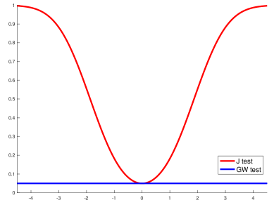
Figure 1: Power of GW and J tests as a function of $c$ when $\varepsilon_{t}$ follows a mean-zero normal distribution.

For this example, $\sqrt{EY^{2}}/\sigma=(1-\rho^{2})^{-1}$, which means that the power of the test based on $J_{T}$ increases in $|\rho|$; in other words, the power of this test is higher for more persistent DGP’s.

It is worth emphasizing that the result in Proposition 5 hinges on using the equal-weighted forecast as our instrument, $h_{t}$. The key point is that although $J_{T}$ and $GW_{T}$ are testing the same MDS null for loss differences, they can have very different power properties for a given choice of instrument.

3.2 Empirical Application

We next illustrate how the insights from our analysis can be used to compare the accuracy of forecasts of two important economic variables, namely US monthly inflation and GDP growth. Specifically, we obtain data from the St. Louis Federal Reserve on the seasonally adjusted consumer price index for all urban consumers (CPIAUCSL) from 1947:01 to 2022:07. From this we compute the monthly inflation rate. Next, we consider the seasonally adjusted Gross Domestic Product (GDP), again obtained from the St. Louis Federal Reserve Fred data base. This is a quarterly series and runs from 1947Q1 through 2022Q2. Again we compute the quarter-over-quarter growth rate and use this as our dependent variable.

For both variables our benchmark models the conditional mean of the dependent variable as a constant while the alternative model uses an AR(4) process. Model parameters are estimated recursively using a 10-year rolling window that gets updated as new data arrive.

As our first instrument, we use the lagged value of the equal-weighted forecast error, i.e., $h_{t}=\xi_{t}=y_{t}-(f_{1,t-1}+f_{2,t-1})/2$. For this case, we obtain test statistics $GW_{T}=1.45$ and $J_{T}=4.56$ for the inflation rate data and $GW_{T}=0.24$ and $J_{T}=2.27$ for the GDP growth data. Hence, in both cases the $J$ test strongly rejects the null while the GW test fails to reject.

The empirical results will of course depend on the chosen instrument. To examine the robustness of our finding, we also consider using instead the difference between the two forecasts as our instrument, setting $h_{t}=f_{1,t-1}-f_{2,t-1}$. Using this instrument, we obtain test statistics $GW_{T}=-1.09$ and $J_{T}=6.18$ for the inflation data and $GW_{T}=-1.30$ and $J_{T}=1.22$ for the GDP growth data. In this case, the $J$ test strongly rejects the null of equal conditional predictive accuracy for the inflation data while the $GW$ test fails to reject. Neither test rejects the null for the GDP growth rate data.

4 Testing Equal Unconditional Expected Predictive Accuracy

So far we have demonstrated that the null that the loss differential follows an MDS generally, though not always, fails to hold conditional on the information set used to generate the forecasts. One might wonder what the GW test is actually testing when the MDS null fails. The obvious candidate is the corresponding unconditional null:

$$H_{0}:\ E[\Delta L_{t+1}]=0.$$ (12)

To examine whether we can use the GW approach to test the null in (12), we separately consider cases with a rolling and an expanding estimation window.

4.1 Rolling estimation window

To see what happens with a rolling estimation window, consider the following simple example:

Example 4.

Suppose that $y_{t+1}=c+\varepsilon_{t+1},$where $\varepsilon_{t}$ is iid with $E\varepsilon_{t}=0$, $E\varepsilon_{t}^{2}=1,$$E\varepsilon_{t}^{3}=\kappa_{1}$ and $E\varepsilon_{t}^{4}=\kappa_{2}$. We use $f_{1,t}=m^{-1}\sum_{s=t-m+1}^{t}y_{t}$ and $f_{2,t}=0$. Assuming squared error loss, we can simply choose $c=m^{-1/2}$ to make the unconditional null hold (i.e., $E(\Delta L_{t+1})=0$).

For the rolling window case, $m$ is fixed and $n$ tends to infinity. Because $m$ is fixed, $\Delta L_{t+1}$ is weakly dependent and stationary. However, the asymptotic distribution of the GW test statistic under the unconditional null hypothesis is not $N(0,1)$. To obtain higher power, GW prefer to use an estimator of the variance of the loss differences that exploits the MDS property of loss differences under the null. However, they also note in Comment 5 that one can use a HAC estimator in situations with, e.g., positive autocorrelation in loss differences. In practice, tests of the unconditional null in (12) are therefore often conducted using an approach similar to that adopted by Diebold and Mariano, (1995) which uses a consistent estimator of the long-run variance of the loss differences and so accounts for any temporal dependencies that may exist.

Using Example 4, we next show that $J_{T}$ converges in distribution to a normal distribution but with variance different from one:

Proposition 6.

In Example 4, $GW_{T}$ converges in distribution to $N(0,V_{m})$, where

$$V_{m}=\frac{4m^{2}-4m^{3/2}\kappa_{1}+m(\kappa_{2}+3)}{8m^{2}+\kappa_{2}-1}.$$

From Proposition 6, the GW test introduces size distortions asymptotically if $V_{m}>1$. This can easily be the case for skewed distributions. For example, let $\log\xi_{t}\sim N(0,\sigma^{2})$ and $\varepsilon_{t}=-(\xi_{t}-E(\xi_{t}))/\sqrt{Var(\xi_{t})}$. Then one can use simulations to see that $V_{m}>3$ for $\sigma=1.5$. Moreover, the asymptotic variance can be arbitrarily close to 1/2 as the rolling window size $m$ increases, leading to an undersized test.

Remark 1.

We can fix this issue by replacing the denominator in $GW_{T}$ with the Newey and West, (1987) or another heteroskedasticity and autocorrelation consistent (HAC) estimator. This is in fact the procedure recommended for the classical test proposed by Diebold and Mariano, (1995). The drawback is that even if $\varepsilon_{t}$ is i.i.d, $\Delta L_{t+1}$ has non-zero autocorrelation for at least $m$ lags. The performance of Newey-West or other HAC estimates might not be satisfactory when the serial dependence in the loss differentials does not decay fast enough.

Remark 2.

Another possibility is to use subsample t-tests similar to those proposed by Ibragimov and Müller, (2010, 2016). Thus, suppose we divide $\{\Delta L_{t+1}\}_{t=m+1}^{m+n}$ into $K$ blocks and let $\Delta\bar{L}^{(k)}$ denote the sample mean of $\Delta L_{t+1}$ in the $k$-th block, $k=1,...,K$. Consider the test statistic

$$S_{K}=\frac{K^{1/2}\overline{\Delta L}}{\sqrt{(K-1)^{-1}\sum_{k=1}^{K}(\Delta\bar{L}^{(k)}-\overline{\Delta L})^{2}}},$$ (13)

where $\overline{\Delta L}=K^{-1}\sum_{k=1}^{K}\Delta\bar{L}^{(k)}$. The limiting distribution of $S_{K}$ is the student $t$-distribution with $K-1$ degrees of freedom.

Remark 3.

It is well known that the outcome of tests of equal unconditional predictive accuracy can be sensitive to the choice of the bandwidth used to estimate the long-run variance of the loss differential, see McCracken, (2020) and Coroneo and Iacone, (2020). Choosing the right bandwidth is often challenging, and McCracken, (2020) finds that very large bandwidths can be required for some data generating processes. An advantage of the above subsample $t$-test is that it does not require a well-defined long-run variance. For example, the variance can change in a non-stationary manner, e.g. with structural breaks, as long as it is bounded.

Proposition 7.

Suppose that $\{\Delta L_{t+1}\}_{t=m+1}^{m+n}$ is stationary and $E\left[\Delta L_{t+1}\right]=0$. Assume that $E|\Delta L_{t+1}|^{r}$ is bounded for some $r>2$ and $\Delta L_{t+1}$ is strong mixing of size $-r/(r-2)$. Then $S_{K}$ converges in distribution to the student $t$-distribution with $K-1$ degrees of freedom.

The self-normalizing feature used to construct the test statistic in (13) means that we do not need to explicitly compute a HAC estimate, although we still need to choose $K$.

The key assumption needed for Proposition 7 is stationarity of the loss difference $\Delta L_{t+1}$. Conversely, the proof does not require us to specify the functional form of the loss (MSE or other loss) and allows for nonlinear models with general estimators computed using a rolling window.

4.2 Monte Carlo simulation results

Consider the setting in Section 4.1. We set $\log\xi_{t}\sim N(0,\sigma^{2})$ and $\varepsilon_{t}=-(\xi_{t}-E(\xi_{t}))/\sqrt{Var(\xi_{t})}$. We report the size of three tests: the original GW test (GW), the Diebold-Mariano test using Newey-West standard errors (DM) and a subsample t-test $S_{K}$ with $K=2$ (Sub). All Monte Carlo experiments are based on 10,000 random samples. To study the asymptotic distribution of the tests, we set the sample size to be a large number ($n=20000$), but we also consider finite-sample performance in samples with $n=100,200$ or 1,000 observations.

Table 1 reports the results. First, consider the performance of the tests in the very large sample ($n=20,000$). The last three columns show that the original GW test tends to have an incorrect size. For $\sigma=0.5$, the original GW test is oversized for small $m$ ($m=3$) and undersized for large $m$ ($m=30$), while both the DM and sub-sampling tests have approximately the right size. For $\sigma=1.5$, we observe serious size distortions for the original GW test which strongly over-rejects. Using Newey-West standard errors improves the accuracy of the GW test but clearly fails to effectively address the issue and this test remains heavily oversized. By far the most accurate test is the subsample t-test of Ibragimov and Müller, (2010, 2016) for which we only see a very small tendency to over-reject (e.g., 6% for a nominal size of 5%). Similar results are seen in the finite samples (columns 1-9) with the original GW and DM Newey-West test statistics tending to over-reject, while the sub-sampling approach is only modestly oversized.

Table 1: Rejection probability of a 5% test under the null hypothesis

	$n=100$			$n=200$			$n=1000$			$n=20000$
	GW	DM	Sub	GW	DM	Sub	GW	DM	Sub	GW	DM	Sub
$m$	$\sigma=0.5$			$\sigma=0.5$			$\sigma=0.5$			$\sigma=0.5$
3	0.0915	0.0860	0.0465	0.0952	0.0792	0.0495	0.0895	0.0580	0.0468	0.0955	0.0530	0.0537
5	0.0742	0.0799	0.0487	0.0737	0.0723	0.0498	0.0725	0.0598	0.0483	0.0755	0.0537	0.0521
10	0.0545	0.0732	0.0524	0.0527	0.0616	0.0505	0.0543	0.0595	0.0517	0.0554	0.0541	0.0496
30	0.0430	0.0604	0.0543	0.0378	0.0500	0.0500	0.0381	0.0452	0.0502	0.0349	0.0435	0.0484
$m$	$\sigma=1$			$\sigma=1$			$\sigma=1$			$\sigma=1$
3	0.2593	0.2022	0.0585	0.2568	0.1748	0.0554	0.2489	0.1217	0.0543	0.2383	0.0725	0.0517
5	0.2282	0.1883	0.0564	0.2364	0.1772	0.0590	0.2368	0.1179	0.0461	0.2589	0.0734	0.0489
10	0.1680	0.1573	0.0510	0.1708	0.1451	0.0506	0.1928	0.1255	0.0508	0.2053	0.0762	0.0508
30	0.1029	0.1182	0.0505	0.1030	0.1059	0.0458	0.1037	0.0946	0.0482	0.1213	0.0854	0.0488
$m$	$\sigma=1.5$			$\sigma=1.5$			$\sigma=1.5$			$\sigma=1.5$
3	0.5324	0.4635	0.1246	0.5196	0.4268	0.1084	0.4942	0.3481	0.0966	0.4182	0.2293	0.0667
5	0.5028	0.4274	0.1091	0.5166	0.4118	0.0969	0.5301	0.3362	0.0896	0.5048	0.2195	0.0640
10	0.4241	0.3819	0.0875	0.4497	0.3754	0.0867	0.5052	0.3362	0.0788	0.5620	0.2218	0.0605
30	0.2698	0.2718	0.0673	0.2979	0.2828	0.0721	0.3523	0.2894	0.0656	0.4707	0.2357	0.0639

4.3 Expanding estimation window

Proposition 2 demonstrates the implausibility of the MDS condition with a rolling window estimation scheme. However, one might wonder whether testing equal predictive accuracy would be easier if one adopts an expanding estimation window. We next examine this point through a simple example:

Example 5.

Consider the following DGP:

$$y_{t}=\varepsilon_{t},$$

where $\{\varepsilon_{t}\}_{t=1}^{T}$ is i.i.d with $E\varepsilon_{t}=0$ and $E\varepsilon_{t}^{2}=1$. Let $\mathcal{F}_{t}$ denote the $\sigma$-algebra generated by $\{\varepsilon_{1},...,\varepsilon_{t}\}$.

Consider an expanding window estimation scheme under which the forecast for $y_{t+1}$ at time $t$ is $f_{1,t}=t^{-1}\sum_{s=1}^{t}y_{s}$, where $t\geq m$ with $m\rightarrow\infty$ and $m/T\rightarrow\lambda$ for $\lambda\in(0,1)$. We compare this forecast with the simple prediction $f_{2,t}=t^{-1/2}$. Clearly, both $f_{1,t}$ and $f_{2,t}$ have a vanishing bias for $E(y_{t+1})=0$. Under squared error loss, one can easily verify that $E(\Delta L_{t+1})=0$ and $E(\Delta L_{t+1}\mid\mathcal{F}_{t})=f_{1,t}^{2}-f_{1,t}^{2}$. Since the bias vanishes with the sample size as the estimation window expands, this example is similar to the local-to-zero setting considered by Clark and McCracken, (2015).

Proposition 8.

In Example 5, the limiting distribution of the GW statistic $GW_{T}$ in (4) is

$$\frac{\int_{\lambda}^{1}(u^{-2}B^{2}(u)-u^{-1})du}{2\sqrt{\int_{\lambda}^{1}\left[u^{-1/2}-u^{-1}B(u)\right]^{2}du}}-\frac{\int_{\lambda}^{1}\left[u^{-1/2}-u^{-1}B(u)\right]dB(u)}{\sqrt{\int_{\lambda}^{1}\left[u^{-1/2}-u^{-1}B(u)\right]^{2}du}},$$ (14)

where $B(\cdot)$ is a standard Brownian motion.

The second term in (14) has a $N(0,1)$ distribution:

$$\frac{\int_{\lambda}^{1}\left[u^{-1/2}-u^{-1}B(u)\right]dB(u)}{\sqrt{\int_{\lambda}^{1}\left[u^{-1/2}-u^{-1}B(u)\right]^{2}du}}\sim N(0,1)\qquad\forall\lambda\in(0,1).$$

Conversely, the first term in (14) has a non-standard distribution and so the limiting distribution of $GW_{T}$ is also non-standard.

In Table 2, we simulate the limiting distribution in (14) and tabulate the 95% quantile of the absolute value limiting distribution for various values of $\lambda$. We also record the asymptotic null rejection probability if we simply choose 1.96 as the critical value (the standard normal limiting distribution stated in GW). We observe substantial size distortions if $\lambda$ is small, even in the limit. Hence, in practice, if the expanding window starts early in the sample, we would falsely reject the null hypothesis too often.

Table 2: Quantiles of the limiting distribution of $|GW_{T}|$ in (14)

$\lambda$	95% quantile	Size if use 1.96
0.05	3.993	0.247
0.10	3.769	0.226
0.15	3.573	0.215
0.20	3.389	0.203
0.25	3.250	0.196
0.30	3.103	0.188
0.35	2.981	0.181
0.40	2.880	0.175
0.45	2.781	0.166
0.50	2.697	0.158
0.55	2.598	0.147
0.60	2.534	0.135
0.65	2.445	0.122
0.70	2.379	0.111
0.75	2.307	0.099
0.80	2.238	0.089
0.85	2.190	0.081
0.90	2.108	0.070
0.95	2.057	0.062
0.99	1.992	0.054

5 Conclusion

Economic forecasts feature prominently in governments’ decisions on fiscal policy, central banks’ monetary policy, households’ consumption and investment decisions and companies’ hiring and capital expenditure choices, so it is important to be able to tell if one forecast can be expected to be more accurate than an alternative forecast. In an influential and innovative paper, Giacomini and White, (2006) develop methods for testing the null hypothesis that two forecasts have identical conditionally expected loss. Equivalently, their null is that the loss differential follows a martingale difference sequence. They use this null to construct a test statistic that does not require Newey-West HAC type adjustments for serial correlation in loss differentials.

The Giacomini-White approach has been used extensively in empirical work as it provides a way to formally compare the accuracy of economic forecasts in situations that are challenging for other tests such as the case with nested models. It turns out that the null that the loss differential is a martingale difference sequence is quite restrictive. We establish that a necessary and sufficient condition for the conditionally expected loss differential of two forecasts to follow an MDS process is that the conditional expectation of the outcome is a simple average of the forecasts. When the underlying forecasts contain parameter estimation errors, this means that the conditional mean of the outcome depends on past estimation errors. One can construct examples where this condition is valid but in many settings of interest to economic forecasters this condition seems hard to justify.

Appendix A Proofs

Proof of Proposition 1.

Notice that

$$\Delta L_{t+1} =(y_{t+1}-f_{1,t})^{2}-(y_{t+1}-f_{2,t})^{2}$$

$$=f_{1,t}^{2}-f_{2,t}^{2}-2y_{t+1}(f_{1,t}-f_{2,t})$$

$$=(f_{1,t}+f_{2,t}-2y_{t+1})(f_{1,t}-f_{2,t}).$$

Since $f_{1,t}$ and $f_{2,t}$ are both $\mathcal{F}_{t}$-measurable, it follows that

$$E(\Delta L_{t+1}\mid\mathcal{F}_{t})=\left[f_{1,t}+f_{2,t}-2E(y_{t+1}\mid\mathcal{F}_{t})\right](f_{1,t}-f_{2,t}).$$

Since $f_{1,t}-f_{2,t}\neq 0$ almost surely, $E(\Delta L_{t+1}\mid\mathcal{F}_{t})=0$ if and only if $f_{1,t}+f_{2,t}-2E(y_{t+1}\mid\mathcal{F}_{t})=0$, which implies $E(y_{t+1}\mid\mathcal{F}_{t})=(f_{1,t}+f_{2,t})/2$. ∎

Proof of Proposition 2.

We proceed by contradiction. Suppose the MDS condition holds, i.e., $E(\Delta L_{t+1}\mid\mathcal{F}_{t})=0$ with probability one. Then by Proposition 1, $E(y_{t+1}\mid\mathcal{F}_{t})=(f_{1,t}+f_{2,t})/2$ almost surely. By the law of iterated expectation, we have

$$E(y_{t+1}\mid\mathcal{F}_{t-m:t})=E\left[E(y_{t+1}\mid\mathcal{F}_{t})\mid\mathcal{F}_{t-m:t}\right]=E\left[(f_{1,t}+f_{2,t})/2\mid\mathcal{F}_{t-m:t}\right]=(f_{1,t}+f_{2,t})/2.$$

Therefore, $E(y_{t+1}\mid\mathcal{F}_{t-m:t})=(f_{1,t}+f_{2,t})/2=E(y_{t+1}\mid\mathcal{F}_{t})$ almost surely. This contradicts the assumption of $P(E(y_{t+1}\mid\mathcal{F}_{t})=E(y_{t+1}\mid\mathcal{F}_{t-m:t}))<1$. The desired result follows. ∎

Proof of Lemma 1.

We proceed by contradiction. Suppose that $E(\Delta L_{t+1}\mid\mathcal{F}_{t})=0$. Let $\hat{\beta}_{t}=(\hat{\beta}_{t,1}+\hat{\beta}_{t,2})/2$ and $\rho=(\rho_{1},...,\rho_{q})^{\prime}$. Then by Proposition 1, we have that $E(Y_{t+1}\mid\mathcal{F}_{t})=(f_{1,t}+f_{2,t})/2=Y_{t-q:t}^{\prime}\hat{\beta}_{t}$. On the other hand, since $Y_{t+1}=\sum_{j=1}^{q}\rho_{j}Y_{t+1-j}+\varepsilon_{t+1}$ and $\varepsilon_{t+1}$ is i.i.d with $E(\varepsilon_{t+1})=0$, we have that $E(Y_{t+1}\mid\mathcal{F}_{t})=Y_{t-q:t}^{\prime}\rho$. Hence, we have $Y_{t-q:t}^{\prime}(\hat{\beta}_{t}-\rho)=0$ almost surely. Therefore, ${\rm Var}\left(Y_{t-q:t}^{\prime}(\hat{\beta}_{t}-\rho)\mid Y_{t-q:t}\right)=0$ almost surely.

However, note that

$${\rm Var}\left(Y_{t-q:t}^{\prime}(\hat{\beta}_{t}-\rho)\mid Y_{t-q:t}\right)=Y_{t-q:t}^{\prime}\left[{\rm Var}(\hat{\beta}_{t,1}+\hat{\beta}_{t,2}\mid Y_{t-q:t})\right]Y_{t-q:t}.$$

Let $\mathcal{A}$ denote the event on which ${\rm Var}(\hat{\beta}_{t,1}+\hat{\beta}_{t,2}\mid Y_{t-q:t})$ is positive definite. Since ${\rm Var}\left(Y_{t-q:t}^{\prime}(\hat{\beta}_{t}-\rho)\mid Y_{t-q:t}\right)=0$ almost surely, it follows that on the event $\mathcal{A}$, $Y_{t-q:t}=0$. Thus, $P(Y_{t-q:t}=0)\geq P(\mathcal{A})$. By assumption, $P(\mathcal{A})>0$, which means that $P(Y_{t-q:t}=0)>0$. However, this is impossible because by assumption $Y_{t-q:t}$ has a density with respect to the Lebesgue measure on $\mathbb{R}^{q}$ and thus $P(Y_{t-q:t}=0)=0$. The proof is complete. ∎

Proof of Proposition 5.

We prove the two claims in two steps.

Step 1: show the result for $GW_{T}$

By $y_{t+1}=(1/2-T^{-1/2}c)y_{t}+\varepsilon_{t+1}$, we have

$$\Delta L_{t+1} =(y_{t+1}-f_{1,t})^{2}-(y_{t+1}-f_{2,t})^{2}$$

$$=(y_{t+1}-y_{t})^{2}-(y_{t+1}-0)^{2}=2T^{-1/2}cy_{t}^{2}-2y_{t}\varepsilon_{t+1}.$$

By $h_{t}=(f_{1,t}+f_{2,t})/2=y_{t}/2$, we have that $\Delta L_{t+1}h_{t}=2T^{-1/2}cy_{t}^{3}-2y_{t}^{2}\varepsilon_{t+1}$. Let $Z_{t+1}=\Delta L_{t+1}h_{t}-E[\Delta L_{t+1}h_{t}\mid\mathcal{F}_{t}]$. Clearly, $\{Z_{t},\mathcal{F}_{t}\}$ is an MDS and $E[\Delta L_{t+1}h_{t}\mid\mathcal{F}_{t}]=2n^{-1/2}cy_{t}^{3}$. Hence,

$$Z_{t+1}=-2y_{t}\varepsilon_{t+1}$$

and

$$EZ_{t+1}^{2}=4\sigma^{2}EY_{t}^{2}.$$

Since $Z_{t}$ is an MDS, we have

$${\rm Var}\left(T^{-1/2}\sum_{t=1}^{n}Z_{t+1}\right)=T^{-1}\sum_{t=1}^{T}E(\Delta L_{t+1}h_{t})^{2}=4\sigma^{2}EY_{t}^{2}.$$

By Theorem 3.35 of White, (2001), $Z_{t+1}$ is stationary and ergodic. By Theorem 3.34 therein, $T^{-1}\sum_{t=1}^{T}Z_{t+1}^{2}=4\sigma^{2}EY_{t}^{2}+o_{P}(1)$. By Corollary 5.26 therein, we have

$$\frac{T^{-1/2}\sum_{t=1}^{T}Z_{t+1}}{2\sigma\sqrt{EY_{t}^{2}}}\rightarrow^{d}N(0,1).$$

In other words, we have $T^{-1/2}\sum_{i=1}^{T}Z_{t+1}\rightarrow^{d}N(0,4\sigma^{2}EY_{t}^{2})$. Again, by Theorems 3.34 and 3.35 of White, (2001), we have

$$T^{-1/2}\sum_{t=1}^{T}E[\Delta L_{t+1}h_{t}\mid\mathcal{F}_{t}]=2cT^{-1}\sum_{i=1}^{T}y_{t}^{3}=2cEY_{t}^{3}+o_{P}(1).$$

Therefore,

$$T^{-1/2}\sum_{t=1}^{T}\Delta L_{t+1}h_{t}\rightarrow^{d}N(2cEY_{t}^{3},4\sigma^{2}EY_{t}^{2}).$$ (15)

On the other hand, by $Z_{t+1}=\Delta L_{t+1}h_{t}-2n^{-1/2}cy_{t}^{3}$, we have that

$$\left|\sqrt{T^{-1}\sum_{t=1}^{T}Z_{t+1}^{2}}-\sqrt{T^{-1}\sum_{t=1}^{T}(\Delta L_{t+1}h_{t})^{2}}\right| \leq\sqrt{T^{-1}\sum_{t=1}^{T}(Z_{t+1}-\Delta L_{t+1}h_{t})^{2}}$$

$$=\sqrt{T^{-1}\sum_{t=1}^{T}(2T^{-1/2}cy_{t}^{3})^{2}}=O_{P}(T^{-1})=o_{P}(1).$$

Since $T^{-1}\sum_{t=1}^{T}Z_{t+1}^{2}=4\sigma^{2}EY_{t}^{2}+o_{P}(1)$, we have

$$T^{-1}\sum_{t=1}^{T}(\Delta L_{t+1}h_{t})^{2}=4\sigma^{2}EY_{t}^{2}+o_{P}(1).$$ (16)

Combining (15) and (16), we have

$$GW_{T}=\frac{T^{-1/2}\sum_{t=1}^{T}\Delta L_{t+1}h_{t}}{\sqrt{T^{-1}\sum_{t=1}^{T}(\Delta L_{t+1}h_{t})^{2}}}\rightarrow^{d}N\left(\frac{cEY_{t}^{3}}{\sigma\sqrt{EY_{t}^{2}}},1\right).$$

Step 2: show the result for $J_{T}$.

The result for $J_{T}$ follows by an analogous argument. We provide a brief proof and point out the difference. Again, define $Z_{t+1}=\xi_{t+1}h_{t}-E[\xi_{t+1}h_{t}\mid\mathcal{F}_{t}]$, where

$$\xi_{t+1}h_{t}=[y_{t+1}-y_{t}/2]\cdot y_{t}/2=\frac{1}{2}y_{t}\varepsilon_{t+1}+\frac{1}{2}n^{-1/2}cy_{t}^{2}$$

and $E[\xi_{t+1}h_{t}\mid\mathcal{F}_{t}]=T^{-1/2}cy_{t}^{2}/2$. Notice that besides a constant factor, the difference from Step 1 is that we now have $y_{t}^{2}$ rather than $y_{t}^{3}$.

By essentially the same argument, we have

$$T^{-1/2}\sum_{t=1}^{T}Z_{t+1}\rightarrow^{d}N(0,\sigma^{2}EY_{t}^{2}/4)$$ (17)

and

$$T^{-1/2}\sum_{t=1}^{T}E[\xi_{t+1}h_{t}\mid\mathcal{F}_{t}]=\frac{1}{2}cT^{-1}\sum_{i=1}^{T}y_{t}^{2}=\frac{1}{2}cEY_{t}^{2}+o_{P}(1).$$ (18)

as well as

$$T^{-1}\sum_{t=1}^{T}(\xi_{t+1}h_{t})^{2}=\sigma^{2}EY_{t}^{2}/4+o_{P}(1).$$ (19)

By (17) and (18), we have that

$$T^{-1/2}\sum_{t=1}^{T}\xi_{t+1}h_{t}=T^{-1/2}\sum_{t=1}^{T}Z_{t+1}+T^{-1/2}\sum_{t=1}^{T}E[\xi_{t+1}h_{t}\mid\mathcal{F}_{t}]\rightarrow^{d}N(cEY_{t}^{2}/2,\sigma^{2}EY_{t}^{2}/4).$$

Then by (19), we have that

$$J_{T}=\frac{T^{-1/2}\sum_{t=1}^{T}\xi_{t+1}h_{t}}{\sqrt{T^{-1}\sum_{t=1}^{T}(\xi_{t+1}h_{t})^{2}}}\rightarrow^{d}N\left(\frac{c\sqrt{EY_{t}^{2}}}{\sigma},1\right).$$

The proof is complete. ∎

Proof of Proposition 3.

To prove this result, we compute the mean squared error for the individual models. To this end, define $y_{(t)}=(y_{2},\cdots,y_{t})^{\prime}\in\mathbb{R}^{t}$ and $\varepsilon_{(t)}=(\varepsilon_{2},\cdots,\varepsilon_{t})^{\prime}\in\mathbb{R}^{t}$. For the small model, $y_{t+1}-f_{1,t}=c+(\beta-\hat{\theta}_{t})x_{t}+\varepsilon_{t+1}$. Since $\hat{\theta}_{t}=x_{(t-1)}^{\prime}y_{(t)}/(x_{(t-1)}^{\prime}x_{(t-1)})$ and $y_{(t)}=c1_{t-1}+x_{(t-1)}\beta+\varepsilon_{(t)}$, we have

$$y_{t+1}-f_{1,t}=c\left(1-\frac{x_{(t-1)}^{\prime}1_{t-1}}{x_{(t-1)}^{\prime}x_{(t-1)}}x_{t}\right)-\frac{x_{(t-1)}^{\prime}\varepsilon_{(t)}}{x_{(t-1)}^{\prime}x_{(t-1)}}x_{t}+\varepsilon_{t+1}.$$

Simple computations yield

$$E\left(y_{t+1}-f_{1,t}\right)^{2}=c^{2}\left(1-\frac{x_{(t-1)}^{\prime}1_{t-1}}{x_{(t-1)}^{\prime}x_{(t-1)}}x_{t}\right)^{2}+\sigma^{2}\left(1+\frac{x_{t}^{2}}{x_{(t-1)}^{\prime}x_{(t-1)}}\right).$$ (20)

For the big model, $y_{t+1}-f_{2,t}=(c-\hat{c}_{t})+(\beta-\hat{\beta}_{t})x_{t}+\varepsilon_{t+1}=\varepsilon_{t+1}-X_{t}^{\prime}\begin{pmatrix}\hat{c}_{t}-c\\ \hat{\beta}_{t}-\beta\end{pmatrix}$. Since $\begin{pmatrix}\hat{c}_{t}-c\\ \hat{\beta}_{t}-\beta\end{pmatrix}=\left(X_{(t-1)}^{\prime}X_{(t-1)}\right)^{-1}X_{(t-1)}^{\prime}\varepsilon_{(t)}$, we have $y_{t+1}-f_{2,t}=\varepsilon_{t+1}-X_{t-1}^{\prime}\left(X_{(t-1)}^{\prime}X_{(t-1)}\right)^{-1}X_{(t-1)}^{\prime}\varepsilon_{(t)}$. By simple computations, we obtain

$$E\left(y_{t+1}-f_{2,t}\right)^{2}=\left(1+X_{t-1}^{\prime}\left(X_{(t-1)}^{\prime}X_{(t-1)}\right)^{-1}X_{t-1}\right)\sigma^{2}.$$ (21)

The first result follows by setting $n^{-1}\sum_{t=m+1}^{m+n}E\left(y_{t+1}-f_{1,t}\right)^{2}=n^{-1}\sum_{t=m+1}^{m+n}E\left(y_{t+1}-f_{2,t}\right)^{2}$ and using (20) and (21).

We now show the second result. Let $\mathcal{F}_{t}$ be the $\sigma$-algebra generated by $(\varepsilon_{1},...,\varepsilon_{t})$ and notice that

$$E\left[\left(y_{t+1}-f_{2,t}\right)^{2}\mid\mathcal{F}_{t}\right]=X_{t-1}^{\prime}\left(X_{(t-1)}^{\prime}X_{(t-1)}\right)^{-1}X_{(t-1)}^{\prime}\varepsilon_{(t)}\varepsilon_{(t)}^{\prime}X_{(t-1)}\left(X_{(t-1)}^{\prime}X_{(t-1)}\right)^{-1}X_{t-1}+\sigma^{2},$$

and

$$E\left[\left(y_{t+1}-f_{1,t}\right)^{2}\mid\mathcal{F}_{t}\right]=\left[c\left(1-\frac{x_{(t-1)}^{\prime}1_{t}}{x_{(t-1)}^{\prime}x_{(t-1)}}x_{t}\right)-\frac{x_{(t-1)}^{\prime}\varepsilon_{(t)}}{x_{(t-1)}^{\prime}x_{(t-1)}}x_{t}\right]^{2}+\sigma^{2}.$$

Therefore,

$$E\left[\Delta L_{t+1}\mid\mathcal{F}_{t}\right]=X_{t-1}^{\prime}\left(X_{(t-1)}^{\prime}X_{(t-1)}\right)^{-1}X_{(t-1)}^{\prime}\varepsilon_{(t)}\varepsilon_{(t)}^{\prime}X_{(t-1)}\left(X_{(t-1)}^{\prime}X_{(t-1)}\right)^{-1}X_{t-1}\\ -\left[c\left(1-\frac{x_{(t-1)}^{\prime}1_{t-1}}{x_{(t-1)}^{\prime}x_{(t-1)}}x_{t}\right)-\frac{x_{(t-1)}^{\prime}\varepsilon_{(t)}}{x_{(t-1)}^{\prime}x_{(t-1)}}x_{t}\right]^{2}.$$

Since $X_{(t-1)}$ contains a column of $1_{t-1}$, there is always a term containing $1_{t-1}^{\prime}\varepsilon_{(t)}$ that cannot be canceled in the above equation. Therefore, it is not possible that with probability one, $E[\Delta L_{t+1}\mid\mathcal{F}_{t}]=0$. Hence, $\Delta L_{t+1}$ is not an MDS. ∎

Proof of Proposition 4.

We proceed in two steps in which we verify the result in the absence and presence of estimation errors.

Step 1: First, ignore estimation errors.

We proceed by contradiction. Suppose that $E(\Delta L_{t+1}\mid\mathcal{F}_{t})=0$ almost surely. In this case, $f_{1,t}=\beta_{1}x_{1t}$ and $f_{2,t}=\beta_{2}x_{2t}$. By Proposition 1, we have

$$E(y_{t+1}\mid\mathcal{F}_{t})=(f_{1,t}+f_{2,t})/2=(\beta_{1}x_{1t}+\beta_{2}x_{2t})/2.$$

However, from the DGP $y_{t+1}=\beta_{1}x_{1t}+\beta_{2}x_{2t}+\varepsilon_{t+1}$ with $E(\varepsilon_{t+1}\mid\mathcal{F}_{t})=0$, we have

$$E(y_{t+1}\mid\mathcal{F}_{t})=\beta_{1}x_{1t}+\beta_{2}x_{2t}.$$

It follows that $\beta_{1}x_{1t}+\beta_{2}x_{2t}=0$ almost surely. This contradicts the assumption, from which the result follows.

Step 2: Next, consider parameter estimation errors.

We proceed by contradiction. Suppose that $E(\Delta L_{t+1}\mid\mathcal{F}_{t})=0$ almost surely. In this case, $f_{1,t}=\hat{\beta}_{1t}x_{1t}$ and $f_{2,t}=\hat{\beta}_{2t}x_{2t}$, where $\hat{\beta}_{1t}$ and $\hat{\beta}_{2t}$ are OLS estimates using information in $\mathcal{F}_{t}$. By Proposition 1, we have

$$E(y_{t+1}\mid\mathcal{F}_{t})=(f_{1,t}+f_{2,t})/2=(\hat{\beta}_{1t}x_{1t}+\hat{\beta}_{2t}x_{2t})/2.$$

On the other hand, we have $E(y_{t+1}\mid\mathcal{F}_{t})=\beta_{1}x_{1t}+\beta_{2}x_{2t}$. This means that $2(\beta_{1}x_{1t}+\beta_{2}x_{2t})=\hat{\beta}_{1t}x_{1t}+\hat{\beta}_{2t}x_{2t}$ almost surely. This contradicts the assumption, from which the result follows. ∎

Proof of Proposition 6.

Let $\bar{\varepsilon}_{t}=m^{-1}\sum_{s=t-m+1}^{t}\varepsilon_{s}$. Then $y_{t+1}-f_{1,t}=\varepsilon_{t+1}-\bar{\varepsilon}_{t}$ and $y_{t+1}-f_{2,t}=c+\varepsilon_{t+1}$. Hence,

$$\Delta L_{t+1}=(y_{t+1}-f_{1,t})^{2}-(y_{t+1}-f_{2,t})^{2}=\bar{\varepsilon}_{t}^{2}-c^{2}-2\varepsilon_{t+1}(c+\bar{\varepsilon}_{t}).$$

Since $m$ is fixed, $\Delta L_{t+1}$ is stationary and weakly dependent; in fact, $\Delta L_{t+1+d}$ and $\Delta L_{t+1}$ are independent for $d\geq m+1$. We next compute the autocovariances, $\gamma_{d}=E\Delta L_{t+1+d}\Delta L_{t+1}$. Clearly, $\gamma_{d}=0$ for $d>m$, so we can focus on $d\leq m$. Since $\varepsilon_{t}$ is iid with mean zero and $c^{2}=m^{-1}$, we observe that

$$\gamma_{d} =E\Delta L_{t+1+d}\Delta L_{t+1}$$

$$=E\left(\bar{\varepsilon}_{t+d}^{2}-c^{2}-2\varepsilon_{t+d+1}(c+\bar{\varepsilon}_{t+d})\right)\left(\bar{\varepsilon}_{t}^{2}-c^{2}-2\varepsilon_{t+1}(c+\bar{\varepsilon}_{t})\right)$$

$$=E(\bar{\varepsilon}_{t+d}^{2}-c^{2})(\bar{\varepsilon}_{t}^{2}-c^{2})-2E(\bar{\varepsilon}_{t+d}^{2}-c^{2})\varepsilon_{t+1}(c+\bar{\varepsilon}_{t})$$

$$=E(\bar{\varepsilon}_{t+d}^{2}-c^{2})(\bar{\varepsilon}_{t}^{2}-c^{2})-2E\bar{\varepsilon}_{t+d}^{2}\varepsilon_{t+1}(c+\bar{\varepsilon}_{t})$$

$$=E(\bar{\varepsilon}_{t+d}^{2}-c^{2})(\bar{\varepsilon}_{t}^{2}-c^{2})-2cE\bar{\varepsilon}_{t+d}^{2}\varepsilon_{t+1}-2E\bar{\varepsilon}_{t+d}^{2}\varepsilon_{t+1}\bar{\varepsilon}_{t}$$

$$=E\bar{\varepsilon}_{t+d}^{2}\bar{\varepsilon}_{t}^{2}-c^{4}-2cE\bar{\varepsilon}_{t+d}^{2}\varepsilon_{t+1}-2E\bar{\varepsilon}_{t+d}^{2}\varepsilon_{t+1}\bar{\varepsilon}_{t}.$$ (22)

The rest of the proof proceeds in three steps.

Step 1: Compute $\gamma_{d}$ for $1\leq d\leq m-1$.

Define $\xi_{1}=\sum_{s=t-m+1}^{t-m+d}\varepsilon_{s}$, $\xi_{2}=\sum_{s=t-m+d+1}^{t}\varepsilon_{s}$ and $\xi_{3}=\sum_{s=t+1}^{t+d}\varepsilon_{s}$. These three quantities are well defined because $1\leq d\leq m-1$. Notice that $\xi_{1}$, $\xi_{2}$ and $\xi_{3}$ are mutually independent with mean zero and satisfy $E\xi_{1}^{2}=d$, $E\xi_{2}^{2}=m-d$ and $E\xi_{3}^{2}=d$. Moreover, $\bar{\varepsilon}_{t+d}=(\xi_{2}+\xi_{3})/m$ and $\bar{\varepsilon}_{t}=(\xi_{1}+\xi_{2})/m$. Therefore, we have

$$E\bar{\varepsilon}_{t+d}^{2}\bar{\varepsilon}_{t}^{2} =m^{-4}E(\xi_{1}+\xi_{2})^{2}(\xi_{2}+\xi_{3})^{2}$$

$$=m^{-4}E(\xi_{1}^{2}+\xi_{2}^{2}+2\xi_{1}\xi_{2})(\xi_{2}^{2}+\xi_{3}^{2}+2\xi_{2}\xi_{3})$$

$$=m^{-4}\left(E\xi_{1}^{2}E\xi_{2}^{2}+E\xi_{1}^{2}E\xi_{3}^{2}+E\xi_{2}^{4}+E\xi_{2}^{2}E\xi_{3}^{2}\right)$$

$$=m^{-4}\left(2dm-d^{2}+E\xi_{2}^{4}\right).$$

Notice that $E\xi_{2}^{4}=\sum_{s_{1}\neq s_{2}}E\varepsilon_{s_{1}}^{2}E\varepsilon_{s_{2}}^{2}+\sum_{s}E\varepsilon_{s}^{4}=(m-d)(m-d-1)+(m-d)\kappa_{2}$. Thus, we have

$$E\bar{\varepsilon}_{t+d}^{2}\bar{\varepsilon}_{t}^{2}=m^{-4}\left(2dm-d^{2}+(m-d)(m-d-1)+(m-d)\kappa_{2}\right)=m^{-4}\left(m^{2}+(m-d)(\kappa_{2}-1)\right).$$ (23)

Since $\bar{\varepsilon}_{t+d}=(\xi_{2}+\xi_{3})/m$, we have

$$E\bar{\varepsilon}_{t+d}^{2}\varepsilon_{t+1}=m^{-2}E(\xi_{2}^{2}+\xi_{3}^{2}+2\xi_{2}\xi_{3})\varepsilon_{t+1}=m^{-2}E\xi_{3}^{2}\varepsilon_{t+1}=m^{-2}E\xi_{t+1}^{3}=m^{-2}\kappa_{1}.$$ (24)

We observe that

$$E\bar{\varepsilon}_{t+d}^{2}\varepsilon_{t+1}\bar{\varepsilon}_{t} =m^{-3}E(\xi_{2}+\xi_{3})^{2}\varepsilon_{t+1}(\xi_{1}+\xi_{2})$$

$$=m^{-3}E(\xi_{2}^{2}+\xi_{3}^{2}+2\xi_{2}\xi_{3})(\xi_{1}+\xi_{2})\varepsilon_{t+1}$$

$$=m^{-3}E(\xi_{2}^{2}+\xi_{3}^{2}+2\xi_{2}\xi_{3})\xi_{2}\varepsilon_{t+1}$$

$$=2m^{-3}E\xi_{2}^{2}\xi_{3}\varepsilon_{t+1}$$

$$=2m^{-3}E\xi_{2}^{2}E\xi_{3}\varepsilon_{t+1}=2m^{-3}(m-d).$$ (25)

Now we combine (22) with (23), (24) and (25), obtaining that for $1\leq d\leq m-1$,

$$\gamma_{d} =m^{-4}(m-d)(\kappa_{2}-1)-2cm^{-2}\kappa_{1}-4m^{-3}(m-d)$$

$$=\left[m^{-4}(\kappa_{2}-1)-4m^{-3}\right](m-d)-2cm^{-2}\kappa_{1}.$$ (26)

Step 2: Compute $\gamma_{d}$ for $d=m$.

We notice that $\bar{\varepsilon}_{t+m}$ and $\bar{\varepsilon}_{t}$ are independent. This means that $E\bar{\varepsilon}_{t+d}^{2}\bar{\varepsilon}_{t}^{2}=m^{-2}=c^{4}$. Moreover, $E\bar{\varepsilon}_{t+d}^{2}\varepsilon_{t+1}=m^{-2}\kappa_{1}$. Finally, $E\bar{\varepsilon}_{t+d}^{2}\varepsilon_{t+1}\bar{\varepsilon}_{t}=E\bar{\varepsilon}_{t+d}^{2}\varepsilon_{t+1}E\bar{\varepsilon}_{t}=0$. It follows by (22) that

$$\gamma_{m}=-2cm^{-2}\kappa_{1}.$$ (27)

Step 3: Compute $\gamma_{d}$ for $d=0$.

We observe that

$$\gamma_{0}=E(\Delta L_{t+1})^{2}=E\left(\bar{\varepsilon}_{t}^{2}-c^{2}-2\varepsilon_{t+1}(c+\bar{\varepsilon}_{t})\right)^{2}=E\left(\bar{\varepsilon}_{t}^{2}-c^{2}\right)^{2}+4E\varepsilon_{t+1}^{2}(c+\bar{\varepsilon}_{t})^{2}\\ =E\bar{\varepsilon}_{t}^{4}-c^{4}+4E(c+\bar{\varepsilon}_{t})^{2}=E\bar{\varepsilon}_{t}^{4}-c^{4}+4(c^{2}+m^{-1})=E\bar{\varepsilon}_{t}^{4}-m^{-2}+8m^{-1}.$$

By a similar argument as in the computation for $E\xi_{2}^{4}$, we can show that $E\bar{\varepsilon}_{t}^{4}=m^{-3}(m-1+\kappa_{2})$. It follows that

$$\gamma_{0}=m^{-3}(\kappa_{2}-1)+8m^{-1}.$$ (28)

Now we apply (26), (27) and (28) and compute the long-run variance

$$\Gamma_{\infty} =\gamma_{0}+2\sum_{d=1}^{\infty}\gamma_{d}$$

$$=\gamma_{0}+2\sum_{d=1}^{m}\gamma_{d}$$

$$=m^{-3}(\kappa_{2}-1)+8m^{-1}$$

$$\qquad+2\sum_{d=1}^{m-1}\left\{\left[m^{-4}(\kappa_{2}-1)-4m^{-3}\right](m-d)-2cm^{-2}\kappa_{1}\right\}+2\times(-2cm^{-2}\kappa_{1})$$

$$=m^{-3}(\kappa_{2}-1)+8m^{-1}-4cm^{-1}\kappa_{1}+2\left[m^{-4}(\kappa_{2}-1)-4m^{-3}\right]\sum_{d=1}^{m-1}(m-d)$$

$$=m^{-3}(\kappa_{2}-1)+8m^{-1}-4cm^{-1}\kappa_{1}+2\left[m^{-4}(\kappa_{2}-1)-4m^{-3}\right]\times\frac{m(m-1)}{2}$$

$$=4m^{-1}-4cm^{-1}\kappa_{1}+m^{-2}(\kappa_{2}+3).$$

By the law of large numbers, $n^{-1}\sum_{t=m+1}^{m+n}(\Delta L_{t+1})^{2}$ converges in probability to $E(\Delta L_{t+1})^{2}=\gamma_{0}$. Therefore, since $c=m^{-1/2},$ the test statistic would have an asymptotic variance equal to

$$\frac{\Gamma_{\infty}}{\gamma_{0}}=\frac{4m^{-1}-4cm^{-1}\kappa_{1}+m^{-2}(\kappa_{2}+3)}{m^{-3}(\kappa_{2}-1)+8m^{-1}}=\frac{4m^{2}-4m^{3/2}\kappa_{1}+m(\kappa_{2}+3)}{8m^{2}+\kappa_{2}-1}.$$

The proof is complete. ∎

Proof of Proposition 7.

Let $Z_{k}=Q^{-1}\sum_{t=m+(k-1)Q+1}^{m+kQ}\Delta L_{t+1}$, where $Q=n/K$. For simplicity, assume that $Q$ is an integer. By Theorem 5.20 of White, (2001) and the Cramer-Wold device, $\sqrt{Q}(Z_{1},...,Z_{K})$ converges in distribution to $(\xi_{1},...,\xi_{K})\sim N(0,c^{2}I_{K})$, where $c^{2}=E(\Delta L_{t})^{2}+2\sum_{s=1}^{\infty}E(\Delta L_{t+s}\Delta L_{t})$. Define the function $g$ by

$$g(\xi_{1},...,\xi_{K})=\frac{K^{1/2}\bar{\xi}}{\sqrt{(K-1)^{-1}\sum_{k=1}^{K}(\xi_{k}-\bar{\xi})^{2}}}$$

with $\bar{\xi}=K^{-1}\sum_{k=1}^{K}\xi_{k}$. Then $S_{K}=g(\sqrt{Q}Z_{1},...,\sqrt{Q}Z_{K})$. The desired result follows by the continuous mapping theorem. ∎

Proof of Proposition 8.

Define $B_{T}(r)=T^{-1/2}\sum_{s=1}^{\left\lfloor rT\right\rfloor}\varepsilon_{s}$. Then by the functional central limit theorem (e.g., Theorem 7.13 of White, (2001)), $B_{T}$ converges weakly to $B$, where $B(\cdot)$ is a standard Brownian motion. In fact, this weak convergence can be strengthened to a strong approximation on a possible extended probability space, i.e., $\sup_{x\in[0,1]}|B_{T}(x)-B(x)|=o_{P}(1)$; see e.g., Theorem 2.1.2 of Csörgo and Révész, (1981).

We notice that $\varepsilon_{t+1}=\sqrt{T}(B_{T}((t+1)/T)-B_{T}(t/T))$ and $f_{1,t}=\sqrt{T}t^{-1}B_{T}(t/T)$. Hence,

$$\Delta L_{t+1} =(\varepsilon_{t+1}-\sqrt{T}t^{-1}B_{T}(t/T))^{2}-(\varepsilon_{t+1}-t^{-1/2})^{2}$$

$$=Tt^{-2}B_{T}^{2}(t/T)-t^{-1}-2\varepsilon_{t+1}(\sqrt{T}t^{-1}B_{T}(t/T)-t^{-1/2})$$

$$=Tt^{-2}B_{T}^{2}(t/T)-t^{-1}-2\sqrt{T}\left[B_{T}((t+1)/T)-B_{T}(t/T)\right]\left(\sqrt{T}t^{-1}B_{T}(t/T)-t^{-1/2}\right).$$ (29)

Therefore,

$$\sum_{t=m}^{T-1}\Delta L_{t+1} =\sum_{t=m}^{T-1}\left(Tt^{-2}B_{T}^{2}(t/T)-t^{-1}-2\sqrt{T}\left[B_{T}((t+1)/T)-B_{T}(t/T)\right]\left(\sqrt{T}t^{-1}B_{T}(t/T)-t^{-1/2}\right)\right)$$

$$=\sum_{t=m}^{T-1}\left((t/T)^{-2}B_{T}^{2}(t/T)-(t/T)^{-1}\right)T^{-1}$$

$$\qquad\qquad-2\sum_{t=m}^{T-1}\left[B_{T}((t+1)/T)-B_{T}(t/T)\right]\left((t/T)^{-1}B_{T}(t/T)-(t/T)^{-1/2}\right)$$

$$=\int_{\lambda}^{1}\left(u^{-2}B^{2}(u)-u^{-1}\right)du-2\int_{\lambda}^{1}\left(u^{-1}B(u)-u^{-1/2}\right)dB(u)+o_{P}(1).$$ (30)

Similarly,

$$\sum_{t=m}^{T-1}(\Delta L_{t+1})^{2}$$

$$=\underset{A_{1,T}}{\underbrace{\sum_{t=m}^{T-1}\left(Tt^{-2}B_{T}^{2}(t/T)-t^{-1}\right)^{2}}}+\underset{A_{2,T}}{\underbrace{4T\sum_{t=m}^{T-1}\left[B_{T}((t+1)/T)-B_{T}(t/T)\right]^{2}\left(\sqrt{T}t^{-1}B_{T}(t/T)-t^{-1/2}\right)^{2}}}$$

$$\qquad-\underset{A_{3,T}}{\underbrace{4\sqrt{T}\sum_{t=m}^{T-1}\left[B_{T}((t+1)/T)-B_{T}(t/T)\right]\left(\sqrt{T}t^{-1}B_{T}(t/T)-t^{-1/2}\right)\left(Tt^{-2}B_{T}^{2}(t/T)-t^{-1}\right)}}.$$

Notice that

$$A_{1,T} =T^{-1}\sum_{t=m}^{T-1}\left((t/T)^{-2}B_{T}^{2}(t/T)-(t/T)^{-1}\right)^{2}T^{-1}$$

$$=T^{-1}\int_{\lambda}^{1}\left(u^{-2}B^{2}(u)-u^{-1}\right)^{2}du+o_{P}(1)=o_{P}(1)$$

and

$$A_{2,T} =4\sum_{t=m}^{T-1}\left[B_{T}((t+1)/T)-B_{T}(t/T)\right]^{2}\left((t/T)^{-1}B_{T}(t/T)-(t/T)^{-1/2}\right)^{2}$$

$$=4\int_{\lambda}^{1}\left(u^{-1}B(u)-u^{-1/2}\right)^{2}du+o_{P}(1).$$

Finally, we observe that

$$A_{3,T}$$

$$=4\sum_{t=m}^{T-1}\left[B_{T}((t+1)/T)-B_{T}(t/T)\right]\left((t/T)^{-1}B_{T}(t/T)-(t/T)^{-1/2}\right)\left((t/T)^{-2}B_{T}^{2}(t/T)-(t/T)^{-1}\right)T^{-1}$$

$$=4\int_{\lambda}^{1}\left(u^{-1}B(u)-u^{-1/2}\right)\left(u^{-2}B^{2}(u)-u^{-1}\right)dB(u)du+o_{P}(1)=o_{P}(1).$$

The above four displays imply that

$$\sum_{t=m}^{T-1}(\Delta L_{t+1})^{2}=4\int_{\lambda}^{1}\left(u^{-1}B(u)-u^{-1/2}\right)^{2}du+o_{P}(1).$$

Therefore, the desired result follows by (30). ∎

References

• Clark and McCracken, (2001) Clark, T. E. and McCracken, M. W. (2001). Tests of equal forecast accuracy and encompassing for nested models. Journal of econometrics, 105(1):85–110.
• Clark and McCracken, (2005) Clark, T. E. and McCracken, M. W. (2005). Evaluating direct multistep forecasts. Econometric Reviews, 24(4):369–404.
• Clark and McCracken, (2015) Clark, T. E. and McCracken, M. W. (2015). Nested forecast model comparisons: a new approach to testing equal accuracy. Journal of Econometrics, 186(1):160–177.
• Coroneo and Iacone, (2020) Coroneo, L. and Iacone, F. (2020). Comparing predictive accuracy in small samples using fixed-smoothing asymptotics. Journal of Applied Econometrics, 35(4):391–409.
• Csörgo and Révész, (1981) Csörgo, M. and Révész, P. (1981). Strong approximations in probability and statistics. Academic Press.
• Diebold and Mariano, (1995) Diebold, F. X. and Mariano, R. S. (1995). Comparing predictive accuracy. Journal of Business & Economic Statistics, pages 253–263.
• Giacomini and White, (2006) Giacomini, R. and White, H. (2006). Tests of conditional predictive ability. Econometrica, 74(6):1545–1578.
• (8) Hansen, P. R. and Timmermann, A. (2015a). Comment on comparing predictive accuracy, twenty years later. Journal of Business and Economic Statistics, 33:17–21.
• (9) Hansen, P. R. and Timmermann, A. (2015b). Equivalence between out-of-sample forecast comparisons and wald statistics. Econometrica, 83(6):2485–2505.
• Ibragimov and Müller, (2010) Ibragimov, R. and Müller, U. K. (2010). t-statistic based correlation and heterogeneity robust inference. Journal of Business & Economic Statistics, 28(4):453–468.
• Ibragimov and Müller, (2016) Ibragimov, R. and Müller, U. K. (2016). Inference with few heterogeneous clusters. Review of Economics and Statistics, 98(1):83–96.
• Inoue and Kilian, (2005) Inoue, A. and Kilian, L. (2005). In-sample or out-of-sample tests of predictability: Which one should we use? Econometric Reviews, 23(4):371–402.
• Lazarus et al., (2018) Lazarus, E., Lewis, D. J., Stock, J. H., and Watson, M. W. (2018). Har inference: Recommendations for practice. Journal of Business & Economic Statistics, 36(4):541–559.
• McCracken, (2007) McCracken, M. W. (2007). Asymptotics for out of sample tests of granger causality. Journal of Econometrics, 140(2):719–752.
• McCracken, (2020) McCracken, M. W. (2020). Tests of conditional predictive ability: Existence, size, and power. FRB St. Louis Working Paper, (2020-050).
• Newey and West, (1987) Newey, W. K. and West, K. D. (1987). A simple, positive semi-definite, heteroskedasticity and autocorrelation-consistent covariance matrix. Econometrica, 55 (3):703–708.
• West, (1996) West, K. D. (1996). Asymptotic inference about predictive ability. Econometrica: Journal of the Econometric Society, pages 1067–1084.
• White, (2001) White, H. (2001). Asymptotic theory for econometricians. New York: Academic Press.