Phase diagram for the bisected-hexagonal-lattice five-state Potts antiferromagnet

Abstract

In this paper we study the phase diagram of the five-state Potts antiferromagnet on the bisected-hexagonal lattice. This question is important since Delfino and Tartaglia recently showed that a second-order transition in a five-state Potts antiferromagnet is allowed, and the bisected-hexagonal lattice had emerged as a candidate for such a transition on numerical grounds. By using high-precision Monte Carlo simulations and two complementary analysis methods, we conclude that there is a finite-temperature first-order transition point. This one separates a paramagnetic high-temperature phase, and a low-temperature phase where five phases coexist. This phase transition is very weak in the sense that its latent heat (per edge) is two orders of magnitude smaller than that of other well-known weak first-order phase transitions.

I Introduction

The $q$-state Potts model Potts_52 ; Wu_82 ; Baxter_book ; Wu_84 is one of most studied models in statistical mechanics, and plays an important role in the theory of phase transitions, especially for two-dimensional (2D) models. Despite its apparent simplicity, no exact solution is known in the whole $(q,T)$ plane, where $q$ is an integer $\geq 2$, and $T\in{\mathbb{R}}$ is the temperature. Instead of the temperature $T$, we will use in this paper the variable

$$v\;=\;v(T)\;=\;e^{J/(k_{B}\,T)}-1\,,$$ (1)

where $J$ is the coupling constant of the Potts model (see Sec. II.1), and $k_{B}$ the Boltzmann constant.

Baxter Baxter_73 ; Baxter_82 ; Baxter_book found the exact free energy on the curve $v=\sqrt{q}$ for the square lattice. This curve has been identified with the critical curve for the ferromagnetic (FM) regime of the model. By universality (see, e.g., Ref. Fisher_98 and references therein), Baxter’s solution implies that the transition is second order for $q\leq 4$, and first order for $q>4$ for any $q$-state FM Potts model defined on any translation-invariant lattice. Universality has allowed researchers to understand the phase diagram of the FM regime of this model, their critical exponents when $q\leq 4$, and their connection with conformal field theories (CFTs) Nienhaus_84 ; DiFrancesco_97 .

From a more practical point of view, the Potts model has applications in condensed-matter systems Wu_82 ; Wu_84 ; Chalker . From a more abstract point of view, the partition function for the $q$-state Potts model on a graph $G$ (see Sec. II.1) is essentially the same as the so-called Tutte polynomial for the graph $G$ Welsh_00 ; Sokal_00 ; handbook_Tutte . This is an object of great interest in combinatorics, as it contains many combinatorial information on the graph $G$. This close connection has allowed the interchange of methods and ideas from one field to the other (see, e.g., Refs. JSS_forests ; JS_flow ).

Unfortunately, the antiferromagnetic regime $v\in[-1,0)$ of the $q$-state Potts model is less well understood, as universality does not hold in general: the phase diagram depends not only on the dimensionality $D=2$ and the number of states $q$, but also on the microscopic structure of the lattice. This implies that the study of this regime has to be done on a case-by-case basis.

There is some kind of “poor man” universality in AF Potts models SS_97a due to the fact that when $q$ is large enough, the system is disordered even at $T=0$. More precisely, for each translation-invariant lattice ${\mathcal{G}}$, there is a value $q_{c}(\mathcal{G})$ such that:

• If $q>q_{c}(\mathcal{G})$, the system is disordered at all temperatures $T\geq 0$.

• If $q=q_{c}(\mathcal{G})$, the system is critical at $T=0$, and disordered at all positive temperatures $T>0$.

• If $q<q_{c}(\mathcal{G})$, any behavior is possible: (a) It can be disordered at all $T\geq 0$ (kagome lattice with $q=2$ Suto1 ; Suto2 ). (b) It can display critical point at $T=0$, and be disordered at any $T>0$ (triangular lattice with $q=2$ Stephenson ). (c) It can undergo a finite-$T$ first-order transition between an ordered phase and a disordered one (triangular lattice with $q=3$ Adler_95 ). (d) It can undergo a finite-$T$ second-order transition between an ordered phase and a disordered one (any bipartite lattice with $q=2$, or the diced lattice with $q=3$ KSS ).

This value $q_{c}(\mathcal{G})$ can be an integer value (like for the square, and kagome lattices with $q_{c}=3$, and for the triangular lattice with $q_{c}=4$); but it can be also a noninteger value (like for the hexagonal lattice: $q_{c}=(3+\sqrt{5})/2$). In the latter case, we should use the Fortuin–Kasteleyn representation FK1 ; FK2 of the $q$-state Potts model to give a rigorous meaning to a $q$-state Potts model with a noninteger value of states. For many lattices, this value is known only approximately: e.g., the diced lattice $q_{c}(\text{diced})\approx 3.45$ JS_unpub , the Union Jack lattice $q_{c}(\text{UJ})=4.326(5)$ union-jack , or the lattices shown in Ref. planar_AF_largeq . Although, it was expected that the maximum value were $q_{c}=4$, this conjecture turned out to be false: there are infinite classes of lattices on which $q_{c}$ is arbitrary large KSS ; planar_AF_largeq . This observation is important in the motivation of this paper.

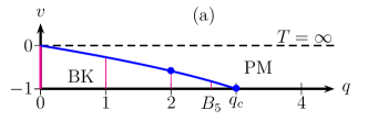
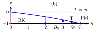
Figure 1: Phase diagram for the AF $q$-state Potts model on the square (a) and on the triangular (b) lattices. The phase labeled PM (resp. BK) represents the paramagnetic (resp. Berker–Kadanoff) phase. Notice that in (b), the region for $q\gtrsim 3.5$ has been distorted to show the diagram more clearly. Regime IV (see text) is colored gray.

The simplest phase diagram for the 2D $q$-state $\mathcal{G}$-lattice AF Potts model is qualitatively similar to that of the square lattice [see Fig. 1(a)]. There is a simple AF critical curve $v_{\text{AF}}(q)$ starting at $(q,v)=(0,0)$ and ending at $(q_{c}(\mathcal{G}),-1)$. The region above this curve and below to the line $v=0$ corresponds to a paramagnetic phase, which is disordered. The region below the curve $v_{\text{AF}}(q)$ and above the line $v=-1$ corresponds to the Berker–Kadanoff phase Saleur_90 ; Saleur_91 . This is a massless phase with algebraic decay of correlations. In fact, this phase exists except when $q$ is a Beraha number $B_{k}$:

$$B_{k}\;=\;4\cos^{2}(\pi/k)\,,\qquad k\;=\;{\mathbb{N}}\setminus\{1\}\,.$$ (2)

At these values, there are massive cancellations of eigenvalues and amplitudes (in the transfer-matrix formalism; see Refs. transfer1 ; transfer2 ; transfer3 ; transfer4 ; transfer_torus ; transfer5 ; transfer6 and references therein), so that the dominant eigenvalue is buried deep inside the spectrum of the corresponding transfer matrix. These values are represented in Fig. 1(a) by pink vertical lines at $B_{2}=0,B_{3}=1,B_{4}=2$, and $B_{5}=(3+\sqrt{5})/2\approx 2.618\,033\ldots$. At these values the thermodynamic limit of the free energy and its derivatives do not commute with the limit $q\to B_{k}$. This phase diagram is also valid for the diced, hexagonal, Union Jack, and BH lattices.

The phase diagram for the 2D $q$-state triangular-lattice AF Potts model is more involved, as it contains an additional element [see Fig. 1(b)]. The AF critical curve $v_{\text{AF}}(q)$ starts at $(q,v)=(0,0)$ with a slope $dv_{\text{AF}}/dq|_{q=0}=-0.1753(2)$ JSS_forests , and moves towards $(q_{c}(\mathcal{G}),-1)$. However, there is a T-point located at $(v_{T},q_{T})$ with $v_{T}=-0.95(2)$ and $q_{T}=3.77(3)$ JSS_tri . At this T-point, the curve $v_{\text{AF}}(q)$ splits into two branches: one goes to the point $(q_{0},-1)$ where $q_{0}=3.819\,671\ldots$ Baxter_86 ; Baxter_87 , and the other branch goes to the point $(q_{c}(\text{tri}),-1)$. This critical curve was first numerically obtained in Ref. JSS_tri using transfer-matrix and critical-polynomial methods Jacobsen_12 ; Scullard_12 ; Jacobsen_13 ; Jacobsen_14 ; Scullard_16 . The Berker–Kadanoff phase has the same properties as for the square-lattice case, and it does not exist for the Beraha numbers $B_{k}$ (2) [in Fig. 1(b) we show these numbers up to $B_{8}$]. At $q=B_{4}=2$ and $q=B_{6}=3$, it is clear that the thermodynamic limit does not commute with the limit $q\to B_{k}$: the AF critical curve does not go through the known critical points for $q=2,3$. In Fig. 1(b), the region for $q\gtrsim 3.5$ has been distorted so that the T-point, as well as the two branches, were visible. The region enclosed by these points correspond to the so-called Regime IV in Ref. Baxter_87 . The conformal properties of this phase were first obtained using a Bethe-Ansatz approach in Ref. Vernier .

In recent years, several “universality classes” in Potts AF have been found:

• If $\mathcal{G}$ is a plane Eulerian triangulation (see Sec. II.2 for details) with one sublattice consisting of vertices of degree $4$, and the other two sublattices are self-dual, then the four-state Potts AF Potts model has a finite-temperature critical point governed by a CFT with central charge $c=3/2$ corresponding to a four-state Potts model and one Ising model (decoupled) union-jack .

• For the same type of triangulations with the exception that the other two sublattices are not self-dual, then the four-state Potts AF Potts model has a finite-temperature critical point governed by a CFT with central charge $c=1$ corresponding to a four-state Potts model union-jack .

• If $\mathcal{G}$ is plane quadrangulation of self-dual type (see Refs. selfdual1 ; selfdual2 for technical details), the three-state Potts AF Potts model has a critical point at $T=0$, and it is disordered for $T>0$.

• If $\mathcal{G}$ is plane quadrangulation of non-self-dual type, the three-state Potts AF Potts model has a finite-temperature phase transition. If this is of second order, it belongs to the universality class of the three-state FM Potts model selfdual1 ; selfdual2 , which is governed by a CFT with $c=4/5$.

The first two examples show that $q_{c}(\mathcal{G})>4$ for any plane Eulerian triangulation $\mathcal{G}$; while the last two examples, show that $q_{c}(\mathcal{G})\geq 3$ for any plane quadrangulation $\mathcal{G}$.

In 2017, Delfino and Tartaglia Delfino_17 used exact methods of 2D field theory to classify the second-order transition points allowed in models with ${\mathbb{S}}_{q}$ symmetry (i.e., $q$-state Potts models). Here $q$ is assumed to be a real parameter. They found several solutions labeled I, II_±, III_±, IV_±, and V_± (Ref. Delfino_17 , Table I). Solution III_- exists for $q\in[0,4]$ and was identified with both the FM critical and tricritical curves of the Potts model. Solution I exists for $q=3$, and is described by a CFT with $c=1$. Actually, a lattice realization of this solution corresponds to the infinitely many models already described in point (c) above selfdual1 ; selfdual2 .

Their solution V is a particularly interesting result: it shows that a second-oder phase transition is allowed for $q\in[4,(7+\sqrt{17})/2]$, where $(7+\sqrt{17})/2\approx 5.561\,552$; and then, in a five-state AF Potts model. The latter can occur on one of the infinitely many possible 2D lattices with $q_{c}>5$ and, since they work in field theory (i.e., directly in the continuum), there is no prediction about which lattice could be a “good” one. While a priori the identification of a “good” lattice seems quite difficult, the results of Ref. union-jack suggested that the bisected-hexagonal (BH) lattice was a good candidate, as $q_{c}(\text{BH})=5.397(5)$, and the results obtained by Monte Carlo (MC) Binder_Landau ; Madras and critical-polynomial methods supported the second-order nature of the transition point. There is a critical point at $v_{c}=-0.915\,32(2)$ with $\gamma/\nu=1.777(3)$, and $\alpha/\nu=1.01(1)$. On the other hand, Ref. planar_AF_largeq contained a detailed study of families of lattices for which $q_{c}$ is arbitrary large. Moreover, for $q\gtrsim 8$, the specific heat diverges, close to the corresponding transition points, like $L^{\approx 2}$. This is the signature of a first-order phase transition for a 2D system Nauenberg_74 ; Klein_76 ; Fisher_82 . However, the behavior for $5\lesssim q\lesssim 8$ was unclear. Therefore, the question of whether the five-state BH-lattice AF Potts model has a second- or first-order phase transition at $v=v_{c}$ is still open.

The goal of this paper is to clarify the order of the transition of the BH-lattice five-state AF Potts model. If second-order, the result would provide a lattice realization of the solution V of Delfino and Tartaglia. If first-order, that would be in accordance with the general behavior found in Ref. planar_AF_largeq . Indeed, if this is the case, it would not mean that the result of Delfino–Tartaglia was false. On the contrary, it would only show that the BH lattice is not a “good” lattice in the above sense, and one has to look for another lattice $\mathcal{G}$ with $q_{c}(\mathcal{G})>5$ that realizes the second-order transition at $q=5$.

We have studied this model by high-precision MC simulations using the well-known and efficient Wang–Swendsen–Kotecký (WSK) algorithm WSK1 ; WSK2 . Unfortunately, the large value of the autocorrelation times close to the transition point (namely, $\tau_{\text{int}}\sim 10^{4}$ for systems of linear size $L=510$), severely limited the maximum size we could simulate with at least $10^{5}\,\tau_{\text{int}}$ Monte Carlo steps (MCS).

First, we have obtained by preliminary MC simulations a “rough” description of the phase diagram of this model. There is a disordered paramagnetic phase when the temperature is large enough (i.e., $v\gtrsim-0.9$). At low temperature, actually at $T=0$, there are exponentially many ground states which lead to a nonzero entropy density. (This provides an exception to the third law of thermodynamics Aizenman ; Chow .) However, at low temperatures, the system is not disordered (as when $q>q_{c}$); but it effectively behaves as having five coexisting phases. The analysis is explained in detail in Appendix B, and it is based on previous models selfdual1 ; selfdual2 for which there is a “height” representation of the corresponding $T=0$ spin models Henley_unpub ; Kondev_96 ; Burton_Henley_97 ; SS_98 ; Jacobsen_09 . Actually, the situation is very close to the low-$T$ phase of the three-state diced-lattice AF Potts model KSS . Therefore, we have two distinct regimes separated by a transition point. For $v<v_{c}$, five phases coexist, and for $v>v_{c}$ there is a unique paramagnetic phase. The question is now to determine the type of the transition at $v=v_{c}$.

The analysis of the MC data has been performed in two complementary ways. On one side, we have analyzed the data using the “standard” approach: i.e., using a general finite-size-scaling (FSS) Ansatz Privmann ; SS_98 (see also Ref. KSS for a more modern application) to fit universal amplitudes like the Binder cumulants or $\xi/L$, where $\xi$ is the (second-moment) correlation length. Indeed, the error bars of all physical quantities were evaluated using the method introduced by Madras and Sokal Madras_Sokal ; Sokal_97 ; Madras that takes into account the correlation among successive measurements. From this analysis we obtained a more precise determination of the transition point $v_{c}$, and an estimate for $y_{t}=2.0(1)$, which agrees well with the predicted value for a first-order phase transition on a 2D system Nauenberg_74 ; Klein_76 ; Fisher_82 . We also estimated the critical-exponent rations $\gamma/\nu$ and $\alpha/\nu$; as well as the dynamic critical exponent $z_{\text{int}}$. However, the results for these exponents were not conclusive.

The other method of analysis is based on the histogram method (see Ref. Lee_91 and references therein), as well as on the use of reweighting techniques (like the Ferrenberg–Swendsen algorithm FS_89 ) and the jackknife method to compute error bars for correlated data Weigel ; Young . For a certain models undergoing a first-order phase transition (including the $q$-state FM Potts model with $q$ large enough), there is a rigorous theory Borgs_90 ; Borgs_91 , which provides support to a previous phenomenological approach Binder_84 ; Challa_86 . Using this approach, we located the (pseudocritical) temperature $v_{\circ}(L)$ for which the energy histogram showed two peaks of equal length. It is interesting to note that for $L\lesssim 48$, this two-peak structure does not exists; and it appears only for $L\gtrsim 96$. By studying the properties of these two-peak histograms, we concluded that the system undergoes a first-order phase transition at $v_{c}$ with a very small latent heat (per edge) $\Delta E=0.000\,48(1)$. This number could be compared to the exact latent heat (per edge) for the five-state FM Potts model on the square lattice $\Delta E=0.026459\ldots$ Baxter_73 , which is the “canonical” example of a weak first-order transition. Moreover, the latent heat (per edge) for the three-state triangular-lattice AF Potts model is $\Delta E=0.0219(5)$ Adler_95 , which is another example of weak first-order transition.

The plan of the paper is as follows. Section II contains the necessary background to make this paper as self-contained as possible. We describe briefly the Potts model, and the geometric properties of the BH lattice. Section III contains information about the physical observables we are going to measure in the MC simulations, as well as details about the efficiency of the WSK algorithm. In Sec. IV, we analyze the MC data using the standard FSS approach without assuming the order of the transition. As the results were not completely conclusive, we include in Sec. V another data analysis based on the histogram method, which has been used quite often to distinguish the order of a transition. Finally in Sec. VI we discuss our findings. In Appendix A, we discuss the question about the right staggering to use in our case. In Appendix B, we study carefully the ground state of our model. This analysis will provide useful insights to understand the physics of this model.

II Basic setup

In this section we will discuss the main topics we will need in the next sections. In Sec. II.1, we summarize the definitions about the $q$-state Potts model, and in Sec. II.2, we describe the BH lattice.

II.1 The $\bm{q}$-state Potts model

The $q$-state Potts model Potts_52 ; Wu_82 ; Baxter_book ; Wu_84 is defined on any undirected graph $G=(V,E)$ with vertex set $V$ and edge set $E$ (in statistical mechanics such graph is usually a finite subset of a regular lattice with certain boundary conditions). On each vertex $x\in V$ of the graph, we place a spin $\sigma_{x}$ that can take any value (or ‘color’) in the set $\Omega=\{1,2,\ldots,q\}$, where $q$ is an integer $q\geq 2$. Each spin $\sigma_{x}$ interacts with the spins $\sigma_{y}$ located on the nearest-neighbor vertices of $x$ with a coupling constant $K\in{\mathbb{R}}$. (Two vertices $x,y\in V$ are nearest neighbors if there is an edge $\{x,y\}\in E$.) The partition function of this model is

$$Z_{G}(q,J)\;=\;\sum\limits_{\sigma\colon V\mapsto\Omega}\exp\left(\beta\sum\limits_{\{x,y\}\in E}\delta_{\sigma_{x},\sigma_{y}}\right)\,,$$ (3)

where the outer sum is over all spin configurations, the sum inside the exponential is over all edges of the graph, $\delta_{a,b}$ is the usual Kronecker $\delta$, and the coupling constant is given by $\beta=J/(k_{B}T)$ (where $k_{B}$ is the Boltzmann constant and $T\geq 0$ is the temperature). If $\beta>0$ (resp. $\beta<0$), the system is in the FM (resp. AF) regime. As we are interested in the AF regime, we will use the more convenient temperature-like parameter $v$ (1), which appears naturally in the Fortuin–Kasteleyn representation of the Potts model FK1 ; FK2 . In the AF regime, $v\in[-1,0)$.

II.2 The bisected-hexagonal lattice

The BH lattice is the Laves lattice $[4,6,12]$, or the dual of the Archimedean lattice $(4,6,12)$ tilings . A BH graph $G_{\text{BH},L}$ of size $L\times L$ and embedded on the torus can be obtained by following the procedure outlined in Ref. union-jack (see also Ref. selfdual2 , Sec. 2.2) with a finite triangular graph $G_{\text{tri},L}$ of size $L\times L$ and embedded on the torus as the starting graph.

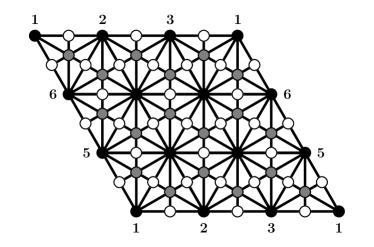
Figure 2: The BH lattice of size $3\times 3$ and periodic boundary conditions. Vertices with the same label should be identified. The three sublattices are shown with different colors (black, gray, and white).

The BH graph $G_{\text{BH},L}=(V_{\text{BH}},E_{\text{BH}})$ is an Eulerian triangulation: i.e., all faces are triangles and all vertices have even degree. The vertex set $V_{\text{BH}}$ can be partitioned into three disjoint subsets $V_{i}$ such that if $\{x,y\}\in E_{\text{BH}}$, then $x,y$ cannot belong to the same subset. Each subset forms a sublattice of $G_{\text{BH},L}$. In Fig. 2, these sublattices are depicted as black, gray, and white dots, respectively. The properties of these sublattices are the following:

• Sublattice $A$ contains the $L^{2}$ vertices of degree $12$, which correspond to the original triangular graph $G_{\text{tri},L}$ of size $L\times L$ (black dots in Fig. 2).

• Sublattice $B$ contains the $2L^{2}$ vertices of degree $6$, and they form the hexagonal graph dual to $G_{\text{tri},L}$ (gray dots in Fig. 2).

• Sublattice $C$ contains the $3L^{2}$ vertices of degree $4$ (white dots in Fig. 2).

To summarize, the linear size of the BH graph $G_{\text{BH},L}$ is defined to be the size of the triangular sublattice $A$. For future convenience, we will assume that $L\equiv 0\pmod{3}$, so that sublattice $A$ is 3-colorable. The smallest of such graphs is depicted in Fig. 2. Then, the number of vertices of $G_{\text{BH},L}$ is $|V_{\text{BH}}|=6L^{2}$, the number of edges is $|E_{\text{BH}}|=18L^{2}$, and the number of triangular faces is $12L^{2}$. In the following, we will denote as $V_{k}$ the vertex set of sublattice $k\in\{A,B,C\}$.

The BH graph can be regarded as a triangular Bravais graph (corresponding to sublattice $A$) with a six-site basis (see Fig. 3). In order to define some physical observables, it is useful to embed the torus in ${\mathbb{R}}^{2}$ with the usual Euclidean distance, and draw the BH graph $G_{\text{BH},L}$ in such a way that it is not distorted and keeps its original symmetries.

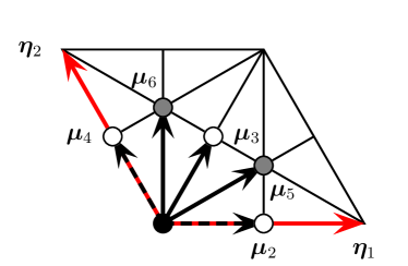
Figure 3: Unit cell of the BH graph. We show the unit vectors $\bm{\eta}_{1}$ and $\bm{\eta}_{2}$ that span the underlying triangular sublattice $A$. We also show the six vectors $\bm{\mu}_{i}$ that define the basis of the this unit cell. The color code of the vertices is as in Fig. 2.

A generic vertex $\bm{x}_{i}$ of the BH graph $G_{\text{BH},L}$ of size $L\times L$ is described geometrically by three numbers $(x^{\prime}_{1},x^{\prime}_{2},k)$ as

$$\bm{x}_{k}\;=\;x^{\prime}_{1}\bm{\eta}_{1}+x^{\prime}_{2}\bm{\eta}_{2}+\sum\limits_{j=1}^{6}\delta_{k,j}\,\bm{\mu}_{j},\;\;x^{\prime}_{1},x^{\prime}_{2}=1,\ldots L.$$ (4)

The vector $\bm{x}^{\prime}=(x^{\prime}_{1},x^{\prime}_{2})^{t}$ lives on a the triangular sublattice $A$ spanned by the (unit) vectors:

$$\bm{\eta}_{1}\;=\;\left(1,0\right)^{t}\,,\qquad\bm{\eta}_{2}\;=\;\left(-\frac{1}{2},\frac{\sqrt{3}}{2}\right)^{t}$$ (5)

and marks the position of the unit cells. The last term in (4) shows the relative position w.r.t. $\bm{x}^{\prime}$ of the vertices in the corresponding unit cell. Thus, the subindex $k$ in $\bm{x}_{k}$ indicates the sublattice the vertex belongs to. Indeed, $\bm{\mu}_{1}=(0,0)^{t}$ for all vertices in sublattice $A$. The two vectors (of norm $1/\sqrt{3}$) associated to the vertices in sublattice $B$ are

$$\bm{\mu}_{5}\;=\;\frac{1}{\sqrt{3}}\,\left(\frac{\sqrt{3}}{2},\frac{1}{2}\right)^{t}\,,\qquad\bm{\mu}_{6}\;=\;\frac{1}{\sqrt{3}}\,\left(0,1\right)^{t}\,.$$ (6)

The three vectors (of norm $1/2$) associated to the vertices in sublattice $C$ are:

$$\bm{\mu}_{2}\;=\;\frac{1}{2}\,\bm{\eta}_{1}\,,\quad\bm{\mu}_{3}\;=\;\frac{1}{2}\,(\bm{\eta}_{1}+\bm{\eta}_{2})\,,\quad\bm{\mu}_{4}\;=\;\frac{1}{2}\,\bm{\eta}_{2}\,.$$ (7)

Therefore, in this geometric representation not all edges have the same length. We will denote a vertex $\bm{x}$ or $x$ depending on whether we are using this geometric representation or not.

III Monte Carlo simulations

This section is devoted to describe the MC simulations we have performed. First, in Sec. III.1, we describe the observables we have measured. In Sec. III.2, we discuss the MC algorithm we have used.

III.1 Physical observables

The simplest observable is the internal energy

$$\mathcal{E}\;=\;\sum\limits_{\{x,y\}\in E_{\text{BH}}}\delta_{\sigma_{x}\sigma_{y}}\,,$$ (8)

where the sum is over all edges in the BH graph.

For the magnetic observables, it is convenient to use the tetrahedral (vector) representation of the spins $\bm{\sigma}_{\bm{x}}\in{\mathbb{S}}^{q-1}$:

$$\bm{\sigma}_{\bm{x}}\;=\;\sum\limits_{\alpha=1}^{q}\delta_{\sigma_{\bm{x}},\alpha}\bm{e}^{(\alpha)}\,,$$ (9)

where the vectors $\bm{e}^{(\alpha)}$ satisfy

$$\bm{e}^{(\alpha)}\cdot\bm{e}^{(\beta)}\;=\;\frac{q\delta_{\alpha\beta}-1}{q-1}\,.$$ (10)

The second observable is the staggered magnetization. In general, the staggering assigns a phase $e^{i\phi_{k}}\in{\mathbb{C}}$ to every vertex belonging to the $k$-th sublattice. Unfortunately, it is not clear a priori what is the right staggering $\phi_{k}$ to choose for the BH lattice when $q=5$. In Appendix A, we have found that a good choice is to consider the magnetization of the spins in sublattice $A$ [cf., Eq. (93)]. Then, we will consider

$$\bm{\mathcal{M}}\;=\;\bm{\mathcal{M}}_{A}\;=\;\frac{1}{V_{A}}\,\sum\limits_{x\in V_{A}}\bm{\sigma}_{x}\,.$$ (11)

We are interested in the squared magnetization given by [cf., (9) and (10)]

$$\bm{\mathcal{M}}^{2}\;=\;\frac{q}{q-1}\,\frac{1}{V_{A}^{2}}\,\sum\limits_{\alpha=1}^{q}\left(\sum\limits_{x\in V_{A}}\delta_{\sigma_{x},\alpha}\right)^{2}-\frac{1}{q-1}\,.$$ (12)

The above observable is a “zero-momentum” one. In order to compute the second-moment correlation length $\xi$, we need to consider the Fourier transform of the spin variables and define the observable $\widetilde{\bm{\mathcal{M}}}(\bm{k})$:

$$\widetilde{\bm{\mathcal{M}}}(\bm{k})\;=\;\frac{1}{V_{A}}\,\sum_{\bm{x}\in V_{A}}\bm{\sigma}_{\bm{x}}\,e^{i\bm{k}.\bm{x}}$$ (13)

evaluated at the smallest allowed nonzero momenta $\bm{k}$. As seen in Sec. II.2, the translation invariance of the BH graph $G_{\text{BH},L}$ is that of the underlying triangular Bravais sublattice $A$. Therefore, the allowed momenta for $G_{\text{BH},L}$ are given by

$$\bm{k}\;=\;\frac{2\pi}{L}\bigl{(}m_{1}\bm{\rho}_{1}+m_{2}\bm{\rho}_{2}\bigr{)}\,,\quad m_{1},m_{2}=1,\ldots,L,$$ (14)

where the momenta basis is given by

$$\bm{\rho}_{1}\;=\;\frac{2}{\sqrt{3}}\,\left(\frac{\sqrt{3}}{2},\frac{1}{2}\right)^{t}\,,\quad\bm{\rho}_{2}\;=\;\frac{2}{\sqrt{3}}\,\left(0,1\right)^{t}\,,$$ (15)

and satisfy [cf., (5)]:

$$\bm{\eta}_{i}\cdot\bm{\rho}_{j}\;=\;\delta_{ij}\,.$$ (16)

The set of the smallest nonzero momenta is

$$\mathcal{K}\;=\;\left\{\pm\frac{2\pi}{L}\bm{\rho}_{1},\pm\frac{2\pi}{L}\bm{\rho}_{2},\pm\frac{2\pi}{L}(\bm{\rho}_{1}-\bm{\rho}_{2})\right\}\,.$$ (17)

The six momenta $\bm{k}\in\mathcal{K}$ have a norm $4\pi/(\sqrt{3}L)$.

Thus, the square of the Fourier transform (13) evaluated at the smallest nonzero momenta is given by

$$\mathcal{F} = \frac{1}{6}\,\sum\limits_{\bm{k}\in\mathcal{K}}\widetilde{\bm{\mathcal{M}}}(\bm{k})^{*}\cdot\widetilde{\bm{\mathcal{M}}}(\bm{k})$$ (18)

$$= \frac{q}{q-1}\,\frac{1}{3}\,\frac{1}{V_{A}^{2}}\sum\limits_{\bm{k}\in\mathcal{K_{+}}}\,\sum\limits_{\alpha=1}^{q}\left|\sum\limits_{\bm{x}\in V_{A}}e^{i\bm{k}\cdot\bm{x}}\,\delta_{\sigma_{\bm{x}},\alpha}\right|^{2},\quad$$

where in the last equation, $\mathcal{K}_{+}\subset\mathcal{K}$ contains the three momenta with positive sign. We have included all the allowed nonzero momenta in $\mathcal{K}_{+}$ to increase the statistics of this observable. [The three momenta with negative sign in $\mathcal{K}$ (17) do not add additional information due to the exact symmetry $\bm{k}\to-\bm{k}$, and can be eliminated to save CPU time.] To obtain the final result (18), we have made use of Eqs. (9) and (10), and the fact that $\bm{k}\neq\bm{0}$ for all $\bm{k}\in\mathcal{K}$.

Starting from the energy (8), we can compute several mean values of interest: the energy density (per edge) $E$, the specific heat $C_{H}$, and the thermal Binder-like ratio $U_{4}$ (Ref. Billoire_Lacaze_Morel_92 , footnote on p. 776):

$$E(v;L) \;=\;\frac{1}{|E_{\text{BH}}|}\,\left\langle\mathcal{E}\right\rangle\,,$$ (19a)

$$C_{H}(v;L) \;=\;\frac{1}{|E_{\text{BH}}|}\,\left\langle(\mathcal{E}-\langle\mathcal{E}\rangle)^{2}\right\rangle\,,$$ (19b)

$$U_{4}(v;L) \;=\;\frac{\left\langle(\mathcal{E}-\langle\mathcal{E}\rangle)^{4}\right\rangle}{\left\langle(\mathcal{E}-\langle\mathcal{E}\rangle)^{2}\right\rangle^{2}}\,,$$ (19c)

where $|E_{\text{BH}}|=18L^{2}$.

The values of $E(v;L)$ and $C_{H}(v;L)$ are easy to obtain in the thermodynamic limit at the extreme cases $v=0$ and $v=-1$. At $v=0$, when the spins are completely uncorrelated, we have that

$$E(0;\infty) \;=\;\frac{1}{q}\;=\;\frac{1}{5}\,,$$ (20a)

$$C_{H}(0;\infty) \;=\;\frac{q-1}{q^{2}}\;=\;\frac{4}{25}\,.$$ (20b)

At $v=-1$, the spin configurations are just proper 5-colorings of the graphs $G_{\text{BH},L}$, and because they are 3-colorable, then $E(-1,\infty)=C_{H}(-1,\infty)=0$. The values of $U_{4}$ (19c) are easy to compute when the energy density can be approximated by a single Gaussian. This is true when the system is in a disordered phase or in an ordered one, but not at the transition point. In the former cases, it attains the same value Tsai_98 :

$$U_{4}(v;\infty)\;=\;3\,,\qquad v\;\neq\;v_{c}\,.$$ (21)

At finite $L$, $U_{4}(v;L)$ displays a minimum close to $v=v_{c}$ Billoire_Lacaze_Morel_92 . If the transition is first order, then this minimum converges to $1$, and to a nontrivial value, if the transition is second order.

In the magnetic sector, we define from (12) and (18) the susceptibility $\chi$, the corresponding “nonzero-momenta” quantity $F$, and the magnetic Binder ratio $R$:

$$\chi(v;L) \;=\;|V_{A}|\,\left\langle\bm{\mathcal{M}}^{2}\right\rangle\,,$$ (22a)

$$F(v;L) \;=\;|V_{A}|\,\left\langle\mathcal{F}\right\rangle\,,$$ (22b)

$$R(v;L) \;=\;\frac{\left\langle(\bm{\mathcal{M}}^{2})^{2}\right\rangle}{\left\langle\bm{\mathcal{M}}^{2}\right\rangle^{2}}\,,$$ (22c)

where $|V_{A}|=L^{2}$.

Notice that our definition of the susceptibility does not contain the connected part as $\langle\bm{\mathcal{M}}\rangle=\bm{0}$ for an infinitely long MC simulation. Therefore, at $v=0$, the susceptibility (22a) takes the value

$$\chi(0;\infty)\;=\;1\,,$$ (23)

and at $v=-1$, it should grow like $L^{2}$. On the other hand, the Binder ratio $R$ has the following limiting values KSS :

$$R(0;\infty) \;=\;\frac{q+1}{q-1}\;=\;\frac{3}{2}\,,$$ (24a)

$$R(-1;\infty) \;=\;1\,,$$ (24b)

where we have assumed that at $T=0$ the system is ordered.

Finally, the second-moment correlation length $\xi$ is defined as

$$\xi(v;L)\;=\;\frac{1}{2\sin(\pi/L)}\,\sqrt{\frac{\chi(v;L)}{F(v;L)}-1}\,.$$ (25)

Indeed, due to our definition of the susceptibility (22a), this formula gives the right correlation length only in the disordered phase. At $v=0$, the correlation length $\xi(v;\infty)$ vanishes. If there is an ordered low-$T$ phase, then we expect that our definition (25) implies that $\xi(-1;L)$ should grow like $L^{2}$.

In order to compute the error bars of $U_{4}$, $R$ and $\xi$, we first compute the variance of the observables SS_00 :

$$\mathcal{O}_{4} \;=\;\frac{(\mathcal{E}-\langle\mathcal{E}\rangle)^{4}}{\langle(\mathcal{E}-\langle\mathcal{E})^{4}\rangle}-2\,\frac{(\mathcal{E}-\langle\mathcal{E}\rangle)^{2}}{\langle(\mathcal{E}-\langle\mathcal{E})^{2}\rangle}+1\,,$$ (26a)

$$\mathcal{O}_{R} \;=\;\frac{\bm{\mathcal{M}}^{4}}{\langle\bm{\mathcal{M}}^{4}\rangle}-2\,\frac{\bm{\mathcal{M}}^{2}}{\langle\bm{\mathcal{M}}^{2}\rangle}+1\,,$$ (26b)

$$\mathcal{O}_{\xi} \;=\;\frac{\bm{\mathcal{M}}^{2}}{\langle\bm{\mathcal{M}}^{2}\rangle}-\,\frac{\mathcal{F}}{\langle\mathcal{F}\rangle}\,.$$ (26c)

Please note that they all have zero mean values. Then the desired standard deviations are given by the following expressions:

$$\sigma(U_{4}) \;=\;U_{4}\,\sigma(\mathcal{O}_{4})\,,$$ (27a)

$$\sigma(R) \;=\;R\,\sigma(\mathcal{O}_{R})\,,$$ (27b)

$$\sigma(\xi) \;=\;\frac{1}{4\sin(\pi/L)}\,\frac{\chi}{F}\,\left(\frac{\chi}{F}-1\right)^{-1/2}\,\sigma(\mathcal{O}_{\xi})\,.$$ (27c)

III.2 The Wang–Swendsen–Koteký algorithm

In order to simulate the five-state AF Potts model on the BH lattice, we have used the algorithm of choice: the Wang–Swendsen–Koteký (WSK) algorithm WSK1 ; WSK2 . This cluster algorithm is a legitimate one for any graph and any positive temperature. The main trouble with the WSK algorithm is that it is not generically ergodic (or irreducible) at $T=0$, where many AF models show interesting physical phenomena. Moreover, it is well known that the WSK algorithm is ergodic at any temperature $T\geq 0$ for any bipartite graph $G$ and for any integer $q\geq 2$ Mohar ; Burton_Henley_97 ; Ferreira_Sokal .

For the majority of the critical points that have being studied using the WSK algorithm, its dynamic behavior overcomes that of single-site algorithms (e.g., Metropolis), which is given by a dynamic critical exponent $z_{\text{int}},z_{\text{exp}}\gtrsim 2$ (see, e.g., Ref. Sokal_97 ).

In particular, for $q=3$ and $G$ being a certain bipartite class of quadrangulations $\mathcal{Q}$ on the torus selfdual1 ; selfdual2 , it has been conjectured (based on strong numerical support) that there is a critical point at $T=0$, but WSK shows no critical slowing down: i.e., $\tau_{\text{int}},\tau_{\text{exp}}\leq A$ uniformly in $v$ and $L$. This was first discovered on the square lattice Ferreira_Sokal ; SS_98 .

Moreover, for $q=3$ and $G$ being any bipartite quadrangulation on the torus not belonging to $\mathcal{Q}$ selfdual1 ; selfdual2 , a similar conjecture has been claimed: there is a finite-temperature critical point, and WSK belongs to the same dynamic universality class as the Swendsen–Wang SW cluster algorithm for the three-state FM Potts model (with $z_{\text{int},\mathcal{M}^{2}}=0.475(6)$ SS_97 ; Garoni_11 ). This phenomenon was first found on the diced lattice KSS .

In addition to these cases, for $q=3$ and the hexagonal lattice it was also found that WSK has no critical slowing down JS_98 . (But this should be expected, as $q_{c}(\text{hex})<3$).

Finally, the three-state AF Potts model on the triangular lattice displays a finite-temperature weak first-order phase transition Adler_95 , so that WSK is expected to perform poorly: i.e., the autocorrelation times are expected to grow exponentially fast $\tau_{\text{int}},\tau_{\text{exp}}\sim e^{2\sigma_{o,d}L}$ for 2D systems, where $\sigma_{o,d}$ is the interface tension Sokal_97 .

For nonbipartite graphs, the question whether WSK is irreducible or not should be investigated on a case-by-case basis. It is worth to note that the lack of ergodicity is usually not a “big” problem on planar graphs: if $G$ is a planar graph with chromatic number $\chi(G)$, then WSK is ergodic for any $q>\chi(G)$ Mohar . In particular, for any finite 3-colorable subset of the BH lattice with e.g., free boundary conditions, WSK is ergodic for any $q\geq 4$; in particular, for $q=5$.

In statistical mechanics, one is interested in graphs embedded on a torus (i.e., periodic boundary conditions) to get rid of surface effects. If we consider finite subsets of nonbipartite translation-invariant lattices $\mathcal{L}$ on the torus, then WSK is not ergodic for important physical cases at $q=q_{c}(\mathcal{L})$: triangular lattices $G_{\text{tri},3L}$ (with $L\geq 2$) at $q=4$ MS1 , kagome lattices $G_{\text{kag},3L}$ (with $L\geq 1$) at $q=3$ MS2 , and even nonbipartite square lattices at $q=3$ Lubin_Sokal .

Moreover, for larger values of $q$, ergodicity may be “restored”: If $\Delta$ is the maximum degree of a graph $G$, then WSK is ergodic for any $q\geq\Delta+1$. In addition, if $G$ is connected and contains a vertex of degree $<\Delta$, then WSK is ergodic for any $q\geq\Delta$ Mohar ; Jerrum . This result implies that WSK is ergodic at $T=0$ on the BH graphs $G_{\text{BH},L}$ for any $q\geq 12\gg 5$. Furthermore, it has been proven that WSK is also ergodic on any triangular (resp. kagome) graph for $q\geq 6$ (res. $q\geq 4$) McDonald ; Bonamy_19 , and there is strong numerical evidence that it is also ergodic for $G_{\text{tri},3L}$ and $q=5$ SS_tri . For the BH lattice, previous MC simulations have located its critical point at $v_{c}=-0.95132(2)>-1$ union-jack , so in principle, we do not have to worry about WSK not being ergodic at $T=0$. However, our past experience with MC simulations for the four-state triangular-lattice AF Potts model SS_tri , has shown that nonergodicity at $T=0$ may induce systematic errors at $T>0$. As $|v_{c}+1|\approx 0.05\ll 1$, this phenomenon cannot be discarded. The slowest mode of the WSK dynamics for the BH graphs $G_{\text{BH},L}$ and $q=5$ is $\bm{\mathcal{M}}^{2}$, as in other similar models Ferreira_Sokal ; SS_98 ; KSS ; selfdual1 ; selfdual2 . Therefore, for each value of $L=3,6,12,24,48,96$, we have made $101$ MC simulations at equidistant values in the range $v\in[-1,-0.9]$ to investigate how the autocorrelation time $\tau_{\text{int},\bm{\mathcal{M}}^{2}}$ behaves as a function of $v$ and $L$ (see Fig. 4). The length of these simulations are in the range $10^{6}$ to $8\times 10^{6}$ MCS; we discarded the first $10\%$ MCS ($\gtrsim 1.2\times 10^{3}\tau_{\text{int},\bm{\mathcal{M}}^{2}}$) to eliminate the initialization bias, and the number of measurements was $\gtrsim 1.1\times 10^{4}\tau_{\text{int},\bm{\mathcal{M}}^{2}}$.

Figure 4 shows that $\tau_{\text{int},\bm{\mathcal{M}}^{2}}$ displays a peak that, as $L$ increases, moves towards the estimate for $v_{c}=-0.95132(2)$, while its width becomes narrower. In the ordered phase, the behavior is rather smooth and the curves for different values of $L$ converge to a value $\tau_{\text{int},\bm{\mathcal{M}}^{2}}\approx 31$ at $T=0$. In the disordered phase, the curves converge as $v\to 0$ (not shown in the figure) to a value $\tau_{\text{int},\bm{\mathcal{M}}^{2}}\approx 3.5$ at $v=0$. This convergence is faster for larger values of $L$. In conclusion, we observe a single peak around the transition point that behaves in the expected way for a critical point. Outside the critical region, it behaves rather smoothly in $v$ and $L$, and converges to fixed values at $v=-1$ and $v=0$. This is empirical evidence that WSK is ergodic on the BH graphs $G_{\text{BH},L}$ for $q=5$ at $T=0$.

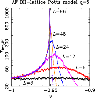
Figure 4: Integrated autocorrelation time $\tau_{\text{int},\bm{\mathcal{M}}^{2}}$ for the five-state BH-lattice AF Potts model in the interval $v\in[-1,-0.9]$. We show data for $L=3$ (black), $L=6$ (red), $L=12$ (pink), $L=24$ (blue), $L=48$ (brown), and $L=96$ (violet). The vertical thin line marks the estimate $v_{c}=-0.95132(2)$ union-jack . Points have been joined with lines to guide the eyes.

We have used the 64-bit linear congruential pseudo-random-number generator proposed by Ossola and Sokal Ossola_Sokal_04a ; Ossola_Sokal_04b . This generator is very simple, is relatively fast, and has been successfully used to obtain high-precision data for the MC simulations of the three-dimensional Ising model ($q=2$) with the Swendsen–Wang algorithm.

In this paper, we have made several fits of the finite-size data of some quantity in order to obtain the relevant physical information. We have used Mathematica’s function NonlinearModelFit to perform the weighted least-squares method for both linear and nonlinear Ansätze. In order to detect corrections to scaling not taken into account in the Ansatz, we have repeated each fit by only allowing data with $L\geq L_{\text{min}}$. We then study the behavior of the estimated parameters as a function of $L_{\text{min}}$. For each fit we report the observed value of the $\chi^{2}$, the number of degrees of freedom (DF), and the confidence level (CL). This quantity is the probability that the $\chi^{2}$ would exceed the observed value, assuming that the underlying statistical model is correct. A “reasonable” CL corresponds to $\text{CL}\gtrsim 10-20\%$, and a very low $\text{CL}\lesssim 5\%$ suggests that this underlying statistical model is incorrect. Commonly, this is due to additional corrections to scaling not taken into account.

Finally, we have performed some simple checks at $v=0$ and $v=-1$ (assuming that WSK is ergodic at this latter temperature).

The values of the observables at $v=0$ have been checked by performing MC simulations on systems of linear sizes $L=3,6,12,24,48$. For the internal energy $E(0;L)$ (19a), the FSS corrections are so small, that a fit to a constant is enough: for $L_{\text{min}}=3$, we already obtain a good fit

$$E(0;\infty)\;=\;0.199999(3)\,,$$ (28)

with $\chi^{2}/\text{DF}=1.75/4$ and $\text{CL}=78\%$. For the specific heat $C_{H}(0;L)$ (19b), we use the same constant Ansatz, and for $L_{\text{min}}=3$, we obtain

$$C_{H}(0;\infty)\;=\;0.1601(2)\,,$$ (29)

with $\chi^{2}/\text{DF}=1.53/4$ and $\text{CL}=82\%$. Finally, the fit for the Binder-like cumulant $U_{4}(0;L)$ (19c) needs an additional FSS correction:

$$U_{4}(0;L)\;=\;U_{4}(0,\infty)+A\,L^{-2}\,.$$ (30)

For $L_{\text{min}}=3$, we obtain

$$U_{4}(0;\infty)\;=\;3.002(4)\,,$$ (31)

with $\chi^{2}/\text{DF}=1.95/3$ and $\text{CL}=58\%$. In all cases, the estimates (28), (29), and (31) agree very well with the exact values (20a), (20b), and (21).

The susceptibility $\chi(0;L)$ (22a), can be well described by a fit to a constant; for $L_{\text{min}}=3$, we obtain the estimate

$$\chi(0;\infty)\;=\;1.0011(9)\,,$$ (32)

with $\chi^{2}/\text{DF}=1.20/4$ and $\text{CL}=88\%$. The fit to the Binder cumulant $R(0;L)$ (22c) needs the Ansatz (30). For $L_{\text{min}}=3$, we get

$$R(0;\infty)\;=\;1.5007(9)\,,$$ (33)

with $\chi^{2}/\text{DF}=2.71/3$ and $\text{CL}=44\%$. Again, the agreement among the estimates (32) and (33) and the exact values (23) and (24a) is also very good.

The values of the observables at $v=-1$ have been obtained from MC simulations on systems of linear sizes $L=3,6,12,24,48,96$. We have fitted the susceptibility $\chi(-1;L)$ (22a) to a power-law Ansatz: for $L_{\text{min}}=24$, we get

$$\chi(-1;L)\;=\;0.8890(3)\,L^{1.99985(7)}\,,$$ (34)

with $\chi^{2}/\text{DF}=0.017/1$ and $\text{CL}=89\%$. The fit for the correlation length $\xi(-1;L)$ (22a) is good if we consider a power-law plus a constant. For $L_{\text{min}}=12$, we obtain

$$\xi(-1;L)\;=\;0.340(2)\,L^{2.001(1)}+2.73(2)\,,$$ (35)

with $\chi^{2}/\text{DF}=0.28/1$ and $\text{CL}=59.8\%$. Finally, the fit of the Binder cumulant $R(-1;L)$ (22c) to the Ansatz (19c), gives for $L_{\text{min}}=24$:

$$R(-1;\infty)\;=\;1.0000002(3)\,,$$ (36)

with $\chi^{2}/\text{DF}=0.122/1$ and $\text{CL}=72\%$. In first two cases, we have checked that the behavior at $v=-1$ is the expected one, namely $\propto L^{2}$, and the value (36) agrees well with the value (24b). It is worth noting that these three results give support to the existence of an ordered phase at low temperature.

IV Numerical results

In this section we will discuss the MC simulations we have done, and the results for the physical quantities of interest. We have followed a similar methodology as in Ref. KSS .

IV.1 Summary of the MC simulations

At every performed MC simulation, we have measured some basic observables $\mathcal{E}$ (8), $\bm{\mathcal{M}}^{2}$ (12), and $\mathcal{F}$ (18). From these measurements, we obtain the basic (static) physical quantities (19), (22), and (25). However, in order to compute their correct error bar, we need to estimate the corresponding integrated autocorrelation times $\tau_{\text{int},\mathcal{O}}$ for $\mathcal{O}\in\{\mathcal{E},\bm{\mathcal{M}}^{2},\mathcal{F}\}$. We have achieved this computation by using the self-consistent algorithm introduced by Madras and Sokal Madras_Sokal ; Sokal_97 (see also Ref. SS_97 ). In this paper, we will call $\tau_{\text{int}}$ the maximum of the measured autocorrelation times $\tau_{\text{int},\mathcal{O}}$.

We have performed several preliminary sets of MC simulations to isolate the regions of interest in $v$, to determine a rough description of the phase diagram, and to check that the dynamic behavior of the WSK algorithm is correct. In these simulations, we focused on the thermal quantities (19), and on the mean magnetization quadratic form $\mathsf{M}$ [c.f., (88)] (we are interested in its dominant eigenvalue and its corresponding eigenvector; see Appendix A for details). These runs were split in several groups:

• We made $101$ runs at equidistant values of $v\in[-1,0]$ for $L=3,6,12,24,48$. They showed that the interesting range was $v\in[-1,-0.9]$, as for $v>-0.9$ the system behaved as it were in a disordered phase (e.g., $U_{4}\approx 3$). In each run, we discarded $\gtrsim 1.3\times 10^{3}\tau_{\text{int}}$ MCS, and took $\gtrsim 1.1\times 10^{4}\tau_{\text{int}}$ measurements.

• We made $101$ runs at equidistant values of $v\in[-1,-0.9]$ for $L=3,6,12,24,48,96$. We obtained that the phase transition was very close to the previous estimate $v_{c}=-0.95132(2)$ union-jack . We could also monitor the behavior of $\tau_{\text{int},\bm{\mathcal{M}}^{2}}$; the result is practically identical to Fig. 4. In each run, we discarded $\gtrsim 1.2\times 10^{3}\tau_{\text{int}}$ MCS, and took $\gtrsim 1.1\times 10^{4}\tau_{\text{int}}$ measurements.

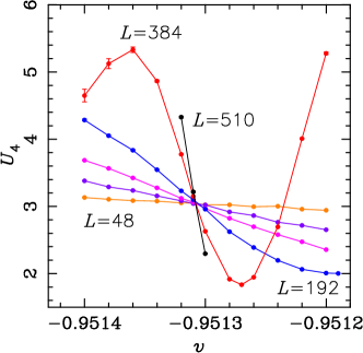
Figure 5: Binder cumulant $U_{4}$ for the five-state BH-lattice AF Potts model in the interval $v\in[-0.95143,-0.95118]$. We show data for $L=48$ (brown), $L=96$ (violet), $L=132$ (pink), $L=192$ (blue), $L=384$ (red), and $L=512$ (black). Points have been joined with lines to guide the eyes.

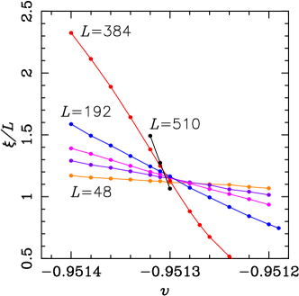
Figure 6: The ratio $\xi/L$ for the five-state BH-lattice AF Potts model in the interval $v\in[-0.95143,-0.95118]$. Color code is as in Fig. 5.

• We made $11$ runs at equidistant values of $v\in[-0.952,-0.951]$ for $L=24,48,96$. We obtained a good choice for the right staggering to use [c.f., (11)/(93)]. Details can be found in Appendix A. We have improved the statistics: we discarded $\gtrsim 10^{4}\tau_{\text{int}}$ MCS, and took $\gtrsim 9.5\times 10^{4}\tau_{\text{int}}$ measurements.

After these preliminary simulations, we then repeated the simulations in (b); but this time, we measured the whole set of thermal (19) and magnetic (22) and (25) observables, as well as their dynamic counterparts (see Fig. 4). The final set of simulations consisted in $11$ equidistant runs in the interval $v\in[-0.952,-0.951]$ for $L=24,48,96,132,192,384$. For $L\leq 132$, we performed MC simulations of lengths in the range $(0.5-2)\times 10^{8}$ MCS, for $L=192$, in the range $(1.1-4.0)\times 10^{8}$ MCS, and for $L=384$, in the range $(2.3-8.7)\times 10^{8}$ MCS. In all cases, we discarded the first $(1.1-1.8)\times 10^{4}\,\tau_{\text{int}}$ MCS; and we took $(1.0-1.6)\times 10^{5}\,\tau_{\text{int}}$ measurements. The results shown in Figs. 5 and 6 for two universal amplitudes, support that the transition was in the interval $v\in[-0.95132,-0.95130]$, so we performed three additional MC simulations at the endpoints and the center of this interval for $L=512$. In these cases, the statistics was smaller: we performed $4\times 10^{8}$ MCS, discarded $\gtrsim 3.6\times 10^{3}\,\tau_{\text{int}}$ MCS, and took $\gtrsim 3.2\times 10^{4}\,\tau_{\text{int}}$ measurements in each of these runs. Notice that the number of spins for $L=510$ is $1.56\times 10^{6}$. The large amount of CPU time needed to perform $10^{8}$ MCS for $L=512$ prevented us from performing more simulations at other values of $v$ for $L=510$, or simulate larger systems for $v\in[-0.95132,-0.95130]$. The numerical MC data can be obtained by request from the corresponding author.

The total amount of CPU time needed for these simulations (plus those reported in Sec. V) was approximately $9.6$ years normalized to an Intel Xeon CPU E5-2687W running at $3.10$ GHz.

IV.2 Determination of the critical point

The goal of this section is to estimate the critical point $v_{c}$ for this model. As mentioned at the end of Sec. IV.1, the interesting interval is $v\in[-0.95132,-0.95130]$. So we have only considered the data points inside it, where the physical quantities are approximately linear functions of $v$.

For each quantity $O=U_{4},R,\xi/L$ shown in Figs. 7–9, we have performed a simultaneous fit of the data with $L\geq L_{\text{min}}$ to the generic Ansatz:

$$O(v;L)\;=\;O_{c}+\sum\limits_{k=1}^{k_{\text{max}}}a_{k}\,(v-v_{c})^{k}\,L^{ky_{t}}\\ +b_{1}\,L^{-\omega_{1}}+\cdots\,,$$ (37)

where the dots represent higher-order FSS corrections. We have varied the number of terms in the Ansatz (37), and the number of data points entering the fit $L\geq L_{\text{min}}$ in order to detect further FSS corrections. In this section, we will not assume any hypothesis on any of the parameters in the Ansatz (37).

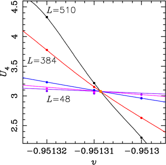
Figure 7: MC results for the Binder ratio $U_{4}$ (19c) in the interval $v\in[-0.951325,-0.951295]$. We show only data for $L\geq 96$ with the color code as in Fig. 5. The solid curves correspond to the actual nonbiased fit, and the golden dot, to our preferred result (38). Note that the values of $U_{4}$ behave monotonically with $L$.

From Fig. 5, it is clear that $U_{4}$ behaves close to the crossing point in a more complicated way than $R$ or $\xi/L$. This explains why we had to use $k_{\text{max}}=4$ in the Ansatz (37). The best fit is obtained by fixing $b_{1}=0$ and taking $L_{\text{min}}=192$. The results are

$$v_{c} \;=\;-0.951\,308\,64(9)\,,$$ (38a)

$$y_{t} \;=\;\phantom{-}2.05(5)\,,$$ (38b)

$$U_{4,c} \;=\;\phantom{-}3.075(3)\,,$$ (38c)

with $\chi^{2}/\text{DF}=1.92/2$ and $\text{CL}=37.7\%$.

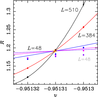
Figure 8: MC results for the Binder ratio $R$ (22c) in the interval $v\in[-0.951325,-0.951295]$. We show only data for $L\geq 96$ with the color code as in Fig. 5. The solid curves correspond to the actual nonbiased fit, and the golden dot, to our preferred result (39). The black (resp. gray) labels refer to the curves (resp. data points).

For the Binder ratio $R$, the best fit is obtained for $k_{\text{max}}=2$, $b_{1}=0$ and $L_{\text{min}}=384$. The results are:

$$v_{c} \;=\;-0.951\,310\,3(6)\,,$$ (39a)

$$y_{t} \;=\;\phantom{-}2.0(1)\,,$$ (39b)

$$R_{c} \;=\;\phantom{-}1.191(4)\,,$$ (39c)

with $\chi^{2}/\text{DF}=0.30/1$ and $\text{CL}=58.5\%$.

Finally, for the ratio $x=\xi/L$, the best fit is obtained for $k_{\text{max}}=1$, $b_{1}=0$, and $L_{\text{min}}=384$. The results are:

$$v_{c} \;=\;-0.951\,307\,2(5)\,,$$ (40a)

$$y_{t} \;=\;\phantom{-}1.84(9)\,,$$ (40b)

$$x_{c} \;=\;\phantom{-}1.218(7)\,,$$ (40c)

with $\chi^{2}/\text{DF}=7.35/5$, and $\text{CL}=19.6\%$.

Notice that our preferred fits for each quantity have a reasonable value of CL in the range $\approx 20-59\%$. For the Binder ratio $U_{4}$, we needed an Ansatz with more terms than usual (e.g., Ref. KSS ). And in all cases, our data did not allow us to determine the leading correction-to-scaling exponent $\omega$ in (37).

Figures 6 and 9 show clearly that $v=-0.95130$ is in the disordered phase, as $\xi/L$ decreases as $L$ increases (contrary to what happens for the other two values of $v$ in Fig. 9). Let us recall that our definition of $\chi$ (22a) does not contain the term $\langle\bm{\mathcal{M}}\rangle^{2}$, so $\chi$ grows with $L$ in the low-$T$ phase. We have $\xi(-0.95130;510)=543(3)\gtrsim L=510$. Therefore, for the linear sizes that we are able to simulate, the correlation length for $v=v_{c}+\epsilon$ is slightly larger than the linear size, so we should expect large corrections to scaling.

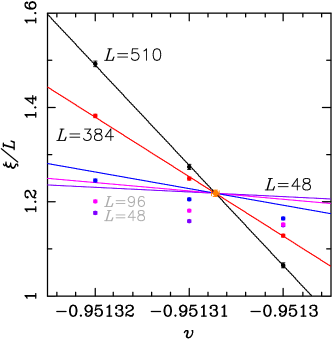
Figure 9: MC results for the ratio $\xi/L$ (25) in the interval $v\in[-0.951325,-0.951295]$. We show only data for $L\geq 96$ with the color code as in Figs. 5 and 8. The solid curves correspond to the actual nonbiased fit, and the golden dot, to our preferred result (40).

Looking at the three distinct estimates for $v_{c}$, we see that the dispersion among them is larger that the error bars. Therefore, if we took into account the statistic and systematic errors, we arrive at the conservative subjective estimate

$$v_{c}\;=\;-0.951\,308(2)\,.$$ (41)

This value agrees within errors with the result obtained in Ref. union-jack using MC simulations $v_{c}=-0.95132(2)$; but our error bar is one order of magnitude smaller. This is a significant improvement.

If we look at the estimates of the thermal RG parameter $y_{t}=1/\nu$, we observe that they all agree within two standard deviations and they are consistently larger than the previous MC estimate $y_{t}=2-X_{t}=1.505(5)$ union-jack . A conservative estimate taking into account both the statistic and systematic errors is

$$y_{t}\;=\;1/\nu\;=\;2.0(1)\,.$$ (42)

This result agrees well with the value expected for a first-order phase transition $y_{t}=2$ in a 2D system Nauenberg_74 ; Klein_76 ; Fisher_82 . If we fix $y_{t}=2$ in the Ansatz (37), we do not get any sizable improvement in the determination of both $v_{c}$ and the universal amplitudes. Finally, $y_{t}=2$ implies the following critical exponents in 2D systems:

$$\nu\;=\;1/2\,,\qquad\alpha\;=\;2-2\nu\;=\;1\,,\quad\alpha/\nu\;=\;2\,.$$ (43)

IV.3 Determination of the static critical exponents

The goal of this section is to estimate the critical- exponent ratios $\alpha/\nu$ and $\gamma/\nu$ for this model. We are going to use the same interval $v\in[-0.95132,-0.95130]$.

For each quantity $O=C_{H},\chi$ shown in Figs. 10 and 11, we have performed a simultaneous fit of the data with $L\geq L_{\text{min}}$ to the generic Ansatz:

$$O(v;L)\;=\;L^{\rho_{O}}\Bigl{[}O_{c}+a_{1}\,(v-v_{c})\,L^{y_{t}}\\ +a_{2}\,(v-v_{c})^{2}\,L^{2y_{t}}+b_{1}\,L^{-\omega_{1}}+\cdots\Bigr{]}\,,$$ (44)

where the dots represent higher-order FSS corrections, and $\rho_{O}$ is the corresponding critical exponent. Again, we have varied both the number of terms in the Ansatz (44), and the number of data points $L\geq L_{\text{min}}$ entering the fit as a precaution against further FSS corrections.

Let us start with the specific heat $C_{H}$. For this quantity, the best results are always obtained from the simplest Ansatz $a_{2}=b_{1}=0$. If we perform this fit without assuming any value for $v_{c}$ and $y_{t}$, the best result corresponds to $L_{\text{min}}=192$:

$$v_{c} \;=\;-0.951\,313(1)\,,$$ (45a)

$$y_{t} \;=\;\phantom{-}2.01(8)\,,$$ (45b)

$$\alpha/\nu \;=\;\phantom{-}1.03(2)\,,$$ (45c)

$$C_{H,c} \;=\;\phantom{-}6.0(6)\times 10^{-4}\,,$$ (45d)

with $\chi^{2}/\text{DF}=1.18/4$, and $\text{CL}=88.2\%$. The value for $v_{c}$ is $2.5$ standard deviations away from our preferred estimate (41); while the value for $y_{t}$ agrees within errors with the estimate (42). Notice that the estimate for the ratio $\alpha/\nu$ is not compatible with the value of $y_{t}$ [cf., (43)].

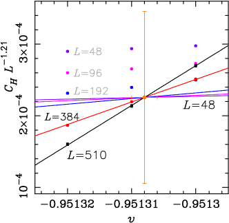
Figure 10: MC results for the ratio $C_{H}/L^{1.21}$ in the interval $v\in[-0.951325,-0.951295]$. We show only data for $L\geq 96$ with the color code as in Figs. 5 and 8. The solid curves correspond to the actual biased fit (46), and the golden dot, to our preferred result (47). The values of $C_{H}/L^{1.21}$ behave monotonically with $L$ on the lhs of the crossing point.

We can try to improve the estimate for $\alpha/\nu$ by performing biased fits by assuming that $v_{c}=-0.951308$ [cf., (41)] and $y_{t}=2$ [cf., (42) and (43)]. In this case, the best fit comes from $L_{\text{min}}=384$:

$$\alpha/\nu\;=\;1.21(2)\,,\quad C_{H,c}\;=\;2.3(3)\times 10^{-4}\,,$$ (46)

with $\chi^{2}/\text{DF}=1.63/3$, and $\text{CL}=65.1\%$. As the error bar in $v_{c}$ is $2\times 10^{-6}$, we have repeated the fits with the values $v_{c}=-0.951306$ and $v_{c}=-0.951310$. We observe that the dispersion in the previous estimates is larger than the corresponding error bars. By taking into account these systematic errors, our best (conservative) estimates are:

$$\alpha/\nu\;=\;1.21(7)\,,\quad C_{H,c}\;=\;2.3(12)\times 10^{-4}\,.$$ (47)

The estimate for $\alpha/\nu$ is $\approx 20\%$ larger than in the nonbiased fit (45); but it is still far away from the expected value for a first-order phase transition $\alpha/\nu=2$. Our final estimate is larger than the previous MC estimate $\alpha/\nu=1.01(1)$ union-jack . Finally, the estimate for the amplitude $C_{H,c}$ is not very precise. The results are depicted in Fig. 10.

We now consider the susceptibility $\chi$ (22a). For this quantity, the best results are always obtained for $b_{1}=0$. If we perform this fit without any further assumption, the best one corresponds to $L_{\text{min}}=192$:

$$v_{c} \;=\;-0.951\,309(1)\,,$$ (48a)

$$y_{t} \;=\;\phantom{-}1.75(6)\,,$$ (48b)

$$\gamma/\nu \;=\;\phantom{-}1.786(9)\,,$$ (48c)

$$\chi_{c} \;=\;\phantom{-}0.92(4)\,,$$ (48d)

with $\chi^{2}/\text{DF}=2.81/3$, and $\text{CL}=42.2\%$. The value for $v_{c}$ agrees within errors with our preferred estimate (41). However, our estimate for $y_{t}$ is $\approx 4$ standard deviations from the estimate (42).

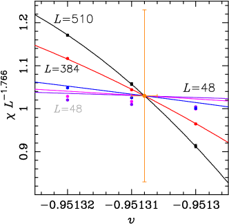
Figure 11: MC results for the ratio $\chi/L^{1.766}$ in the interval $v\in[-0.951325,-0.951295]$. We show only data for $L\geq 96$ with the color code as in Figs. 5 and 8. The solid curves correspond to the actual biased fit (49), and the golden dot, to our preferred result (50).

Again, we may improve the estimate for $\gamma/\nu$ by performing biased fits by assuming that $v_{c}=-0.951308$ [cf., (41)] and $y_{t}=2$ [cf., (42) and (43)]. In this case, the best fit comes from $L_{\text{min}}=384$:

$$\gamma/\nu\;=\;1.766(9)\,,\qquad\chi_{c}\;=\;1.03(6)\,,$$ (49)

with $\chi^{2}/\text{DF}=1.09/2$, and $\text{CL}=58.0\%$. Again, by repeating the fits with $v_{c}=-0.951306$ and $v_{c}=-0.951310$, we observe that the dispersion among the estimates is larger than their statistical errors. By taking into account this dispersion, our best estimates are:

$$\gamma/\nu\;=\;1.77(4)\,,\qquad\chi_{c}\;=\;1.0(2)\,.$$ (50)

The estimate for $\gamma/\nu$ agrees within errors with that from the nonbiased fit (48), but it is still $\lesssim 6$ standard deviations from the expected value $\gamma/\nu=2$ for a first-order phase transition. On the other hand, our final estimate agrees within errors with the value quoted in the literature $\gamma/\nu=1.774(8)$ union-jack . Finally, our estimate for the amplitude $\chi_{c}$ is not very precise (see Fig. 11).

IV.4 Determination of the dynamic critical exponents

The goal of this section is to study how the integrated autocorrelation time for the slowest mode of the WSK algorithm (i.e., $\tau_{\text{int},\bm{\mathcal{M}}^{2}}$) behaves close to the critical point $v_{c}$. In particular, we would like to tell whether $\tau_{\text{int},\bm{\mathcal{M}}^{2}}\sim L^{z_{\text{int},\bm{\mathcal{M}}^{2}}}$, or $\tau_{\text{int},\bm{\mathcal{M}}^{2}}\sim L^{2\sigma_{o,d}\,L}$. Again, we will focus on the interval $v\in[-0.95132,-0.95130]$.

In this case, we have performed biased fits to two different Ansätze: a power-law one like in (44), and an exponential one in which the term $L^{\rho_{O}}$ in (44) has been replaced by $e^{2\sigma_{o,d}L}$.

In the first case, our preferred fit corresponds to $a_{2}=b_{1}=0$ and $L_{\text{min}}=384$:

$$z_{\text{int},\bm{\mathcal{M}}^{2}}\;=\;1.54(6)\,,\qquad\tau_{c}\;=\;0.6(2)\,,$$ (51)

with $\chi^{2}/\text{DF}=3.86/3$, and $\text{CL}=27.7\%$. We have repeated the fits with $v_{c}=-0.951306$ and $v_{c}=-0.951310$, and in this case, the dispersion of the estimates is only slightly larger than the error bars:

$$z_{\text{int},\bm{\mathcal{M}}^{2}}\;=\;1.54(6)\,,\qquad\tau_{c}\;=\;0.6(3)\,.$$ (52)

The results are shown in Fig. 12.

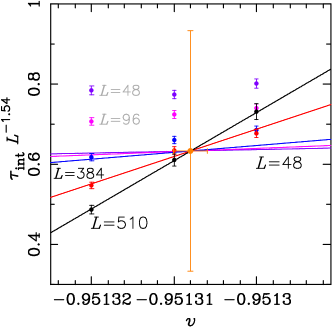
Figure 12: MC results for the integrated autocorrelation time $\tau_{\text{int},\bm{\mathcal{M}}^{2}}/L^{1.54}$ in the interval $v\in[-0.951325,-0.951295]$. We show only data for $L\geq 96$ with the color code as in Figs. 5 and 8. The solid curves correspond to the actual biased fit (51), and the golden dot, to our preferred result (52).

If we consider the exponential Ansatz, we also obtain the best estimates for $a_{2}=b_{1}=0$ and $L_{\text{min}}=384$:

$$2\sigma_{o,d}\;=\;0.0035(1)\,,\qquad\tau_{c}\;=\;1.63(9)\times 10^{4}\,,$$ (53)

with $\chi^{2}/\text{DF}=3.86/3$, and $\text{CL}=27.7\%$. Again, we have repeated the fits with $v_{c}=-0.951306$ and $v_{c}=-0.951310$, and in this case, the dispersion of the estimates is smaller than the error bars quoted in (53). The results are displayed in Fig. 13.

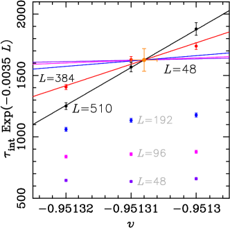
Figure 13: MC results for the integrated autocorrelation time $\tau_{\text{int},\bm{\mathcal{M}}^{2}}e^{-0.0035L}$ in the interval $v\in[-0.951325,-0.951295]$. We show only data for $L\geq 96$ with the color code as in Figs. 5 and 8. The solid curves correspond to the actual biased fit (53), and the golden dot, to our preferred result (53).

The quality of the fits (51)/(53) is the same, so we do not have arguments in favor of any of the two Ansätze. The power-law Ansatz implies that the dynamic critical exponent (51) is somewhat smaller than the exponent associated to single-site algorithms $\gtrsim 2$. On the other hand, the exponential Ansatz predicts a very small interface tension (53).

V Histogram analysis

In the previous section we have seen several indications that the transition undergone by the five-state BH-lattice AS Potts model was first order, but there were other estimates pointing to the second-order nature of that transition. The use of histograms for analyzing simulations has a long story (see e.g., the list of references in Ref. Lee_91 ). Actually, for certain class of models (that include the $q$-state FM Potts model at large $q$) there is a rigorous theory Borgs_90 ; Borgs_91 (see also Ref. Lee_91 ). In particular, it was proven that for the 2D $q$-state FM Potts model at large $q$, the partition function can be written as

$$Z(\beta;L)\;=\;e^{-L^{2}\beta f_{d}(\beta)}+qe^{-L^{2}\beta f_{o}(\beta)}\\ +O\Bigl{(}e^{-bL}\Bigr{)}e^{-L^{d}\beta f(\beta)}\,,$$ (54)

for some positive constant $b>0$. In Eq. (54), periodic boundary conditions are assumed, $f_{d}(\beta)$ and $f_{o}(\beta)$ are smooth functions independent of $L$, and $f(\beta)=\min(f_{d}(\beta),f_{o}(\beta))$. The free energy of the model is given by $f_{o}(\beta)$ (resp. $f_{d}(\beta)$) when $\beta\geq\beta_{c}$ (resp. $\beta\leq\beta_{c}$). By using an inverse Laplace transform Billoire_94 , one can recover the phenomenological two-Gaussian Ansatz introduced by Binder, Challa, and Landau Binder_84 ; Challa_86 , with the correct weight for the Gaussians.

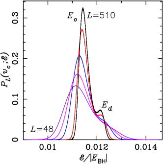
Figure 14: Energy histograms for the five-state BH-lattice AF Potts model at the critical point $v_{c}=-0.951\,308$ [cf., (41)] for $L=96$ (violet), $L=132$ (pink), $L=192$ (blue), $L=384$ (red), and $L=510$ (black). The label $E_{o}$ (resp. $E_{d}$) shows the energy peak for the ordered (resp. disordered) phase. The peak at $E_{o}$ becomes higher and narrower as $L$ increases.

One may think that a priori the five-state BH-lattice AF Potts model does not allow the use of the histogram method: it is an AF model with a nonzero entropy density at $T=0$. However, this might not be the case: the results discussed in Appendix B indicate that this model has an ordered low-$T$ phase in which five distinct phases coexist. This situation is similar to the one found for the three-state diced-lattice AF Potts model KSS . For that model, a contour analysis was used to prove the existence of a finite-$T$ phase-transition point (see also Ref. Kotecky-Sokal-Swart for more details and generalizations). In conclusion, we consider it makes sense to use the histogram method to study the nature of the phase transition of our model. Furthermore, we were able to find two peaks in the energy probability distribution $P_{L}(v;\{\mathcal{E}\})$ for some of the MC simulations described in Sec. IV. However, as shown in Ref. Lee_90 , a two-peak signal does not always imply a first-order phase transition: one has to analyze carefully how these peaks behave as $L$ is increased.

First, we have extrapolated the MC histograms at $v=-0.95131$ for $L\geq 96$ to the bulk critical point $v_{c}=-0.951\,308$ [cf., (41)] using the Ferrenberg–Swendsen FS_89 method. The probability distributions shown in Fig. 14 have been normalized in the following way. First, the energy $\mathcal{E}$ has been normalized as in Eq. (19a), so it varies in the interval $[0,1]$. On the other hand, the number of values the energy can take in each simulation increases with $L$ (see below). Therefore, the “raw” probability distributions cannot be compared directly. In order to be able to do so, we have divided the whole interval $\mathcal{E}/|E_{\text{BH}}|\in[0,0.2]$ (where the internal energy is constrained close to the critical temperature) into $100$ bins, and recompute the probability distributions with this new common bin size. In this way we obtain the right normalization factor for each histogram, such that they can be compared when plotted all together as in Fig. 14. It is clear that there is a single peak for $L\lesssim 192$; but for $L=384$ we see a small plateau that develops into a small “bump” for $L=510$. So, from the study of the histograms at $v=v_{c}$, we see that $L=510$ is actually too small for our model to show a clear double-peak structure (if any).

V.1 Analysis when the peaks have the same height

As noted in Ref. Borgs_92 , at the point $v_{C_{H,\text{max}}}$ where the specific heat $C_{H}(v_{C_{H,\text{max}}};L)$ attains its maximum value, the energy probability distribution $P_{L}(v_{C_{H,\text{max}}};\mathcal{E})$ typically shows two peaks of similar heights. This phenomenon is also observed in our system, but only when $L\geq 96$. For $L=48$, we find only a broad peak; but not two peaks. This means that if the transition is first order, then we need to study systems with linear sizes $L\geq 96$. In practice, we made a long MC simulation close to that point, and then used the Ferrenberg–Swendsen method to find the point $v_{\circ}(L)$ for which the heights of these two peaks were equal. This method of locating the temperature for which the energy histogram displays two equal peak has been successfully used in the literature to study first-order phase transitions Lee_90 ; Lee_91 ; Janke_93 ; Janke_94 . One good property of this method is that we do not need the exact position of the bulk critical temperature $v_{c}$.

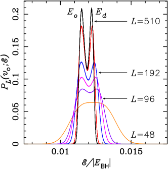
Figure 15: Energy histograms for the five-state BH-lattice AF Potts model at $v=v_{\circ}(L)$ for $L\geq 48$. The color code is as in Fig. 14. See Table 1 for the values of $v_{\circ}(L)$. The label $E_{o}$ (resp. $E_{d}$) shows the energy peak for the ordered (resp. disordered) phase.

For $L=48$ we made a long MC simulation at the point $v_{\circ}=-0.95029$ where the histogram displayed a broad peak (see Fig. 15). For the other values of $L=96,132,192,384,510$, we have performed a long MC simulation at a temperature $v_{1}$, for which the histogram showed a two-peak structure, but with unequal heights; we then used the Ferrenberg–Swendsen method to locate the nearby temperature $v_{\circ}(L)$ for which the histogram had two peaks of identical height. The probability distributions shown in Fig. 15 have been normalized as in Fig. 14.

The values of $v_{1}$ and $v_{\circ}$ are displayed on the second and third columns of Table 1. The length of each MC simulation (“MCS”), the number of discarded MCS (“Disc.”), and the number of measurements (“Meas.”) are also displayed in Table 1. For $48\leq L\leq 384$, we have discarded $\gtrsim 1.1\times 10^{4}\,\tau_{\text{int},\bm{\mathcal{M}}^{2}}$, and taken $\gtrsim 10^{5}\,\tau_{\text{int},\bm{\mathcal{M}}^{2}}$ measures. The statistics for $L=510$ is smaller: we have discarded $\gtrsim 3.6\times 10^{3}\,\tau_{\text{int},\bm{\mathcal{M}}^{2}}$, and taken $\gtrsim 3.2\times 10^{4}\,\tau_{\text{int},\bm{\mathcal{M}}^{2}}$, measures.

$L$	$v_{1}$	$v_{\circ}$	MCS	Disc.	Meas.
48	$-0.95029$		$2\times 10^{8}$	$\phantom{1}2\times 10^{7}$	$1.8\times 10^{8}$
96	$-0.95095$	$-0.950955(1)$	$2\times 10^{8}$	$\phantom{1}2\times 10^{7}$	$1.8\times 10^{8}$
132	$-0.95110$	$-0.951098(1)$	$2\times 10^{8}$	$\phantom{1}2\times 10^{7}$	$1.8\times 10^{8}$
192	$-0.95119$	$-0.951193(1)$	$4\times 10^{8}$	$\phantom{1}4\times 10^{7}$	$3.6\times 10^{8}$
384	$-0.95127$	$-0.9512722(2)$	$9\times 10^{8}$	$10\times 10^{7}$	$8.0\times 10^{8}$
510	$-0.95130$	$-0.9512864(2)$	$4\times 10^{8}$	$\phantom{1}4\times 10^{7}$	$3.6\times 10^{8}$

Table 1: For each value of $L=48,96,132,192,384,510$, we show the temperature $v_{1}$ where the MC simulation was performed, the temperature $v_{\circ}(L)$ for which the extrapolated probability distribution $P_{L}(v_{\circ};\{\mathcal{E}\})$ shows a two-peak structure with peaks of the same height, the total number of MCS, the number of discarded initial steps (“Disc.”), and the number of performed measures (“Meas.”).

We have followed a procedure to estimate the quantities displayed in Table 1 which is based on the Ferrenberg–Swendsen algorithm and on the jackknife method to estimate the error bars (see e.g. Ref. Weigel ; Young and references therein).

First, for each MC simulation performed at $v_{1}=v_{1}(L)$, we store the measured energy $\mathcal{E}$ into $N=20$ histograms $H_{L}^{(i)}=H_{L}^{(i)}(v_{1}(L);\{\mathcal{E}\})$. The $j$-th bin $H_{L}^{(i)}(\mathcal{E}_{j})$ of the $i$-th histogram $H^{(i)}_{L}$ contains the number of times the energy value $\mathcal{E}_{j}\in\Delta{\mathcal{E}}(L)=[\mathcal{E}_{\text{min}}(L),\mathcal{E}_{\text{max}}(L)]$ has appeared in the $i$-th part of that MC simulation. Indeed, the probability distribution of the energy is given by

$$P^{(i)}_{L}(v_{1};\mathcal{E}_{j})\;=\;\frac{H_{L}^{(i)}(v_{1};\mathcal{E}_{j})}{\sum\limits_{\mathcal{E}_{k}\in\Delta{\mathcal{E}}(L)}H_{L}^{(i)}(v_{1};\mathcal{E}_{k})}\,.$$ (55)

Each histogram $H_{L}^{(i)}$ contains $\gtrsim 5\times 10^{3}\,\tau_{\text{int},\bm{\mathcal{M}}^{2}}$ measures for $L\leq 384$, and $\gtrsim 1.6\times 10^{3}\,\tau_{\text{int},\bm{\mathcal{M}}^{2}}$ measures for $=510$. Due to the large values for the autocorrelation times for the WSK algorithm, this choice is a compromise between a number of blocks of order $10^{2}$, and a size of each block of order $10^{4}\tau_{\text{int}}$ needed to apply the jackknife method according to Ref. Weigel . The number of energy values $\delta E(L)=\mathcal{E}_{\text{max}}(L)-\mathcal{E}_{\text{min}}(L)$ increases with $L$: $\delta E(96)=991$, $\delta E(132)=1451$, $\delta E(192)=2459$, $\delta E(384)=6500$, and $\delta E(510)=9521$.

Let us fix $L$, and suppose that, if we extrapolate the histograms $H^{(i)}_{L}(v_{1})$ to a nearby temperature $v_{\circ}$, we get a two-peak structure with peaks of equal height. Then we performed the following procedure to extract the relevant physical information:

1. First, we obtained the probability distributions $P_{L}^{(i)}(v_{1};\{\mathcal{E}\})$ using (55). The total probability distribution is given by

   $$P_{L}(v_{1};\{\mathcal{E}\})\;=\;\frac{1}{N}\,\sum\limits_{i=1}^{N}P^{(i)}_{L}(v_{1};\{\mathcal{E}\})$$ (56)

   because the normalization of every histogram is the same and equal to the total number of measurements. The computations in this procedure have been carried out using Mathematica with 50-digit precision.

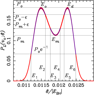
Figure 16: Energy histogram for the five-state BH-lattice AF Potts model at $v=-0.9512722$ for $L=385$ (red). The blue curves are the actual fits around the two peaks and the valley. We show the limits where these fits were performed. See point (d) for an explanation of the labels.

1. We then obtained the extrapolated probability distributions $P_{L}^{(i)}(v_{\circ};\{\mathcal{E}\})$ at $v=v_{\circ}$ using the Ferrenberg–Swendsen method. Likewise, we obtain the total probability distribution $P_{L}(v_{\circ};\{\mathcal{E}\})$.

2. We also needed an estimate of the error bars in the values of $P_{L}(v_{\circ};\mathcal{E}_{j})$ for each $\mathcal{E}_{j}\in\Delta\mathcal{E}(L)$. We used the jackknife method to compute such error bars. Due to the large amount of data involved, we assumed that each bin was statistically independent of the other bins, i.e., $\operatorname{\mathrm{cov}}(P_{L}(v_{\circ};\mathcal{E}_{j}),P_{L}(v_{\circ};\mathcal{E}_{k}))=0$ for any $j\neq k$. Indeed, the jackknife estimate for the mean value of the $j$-th bin coincides with $P_{L}(v_{\circ};\mathcal{E}_{j})$, so we recorded the corresponding error bars $\sigma(P_{L}(v_{\circ};\mathcal{E}_{j}))$. The assumption of neglecting the off-diagonal terms of the covariance matrix is not true in general, so our error bars might be either underestimated or overestimated. This is a warning in order to interpret correctly the following fits.

3. The next step was to locate the position of both peaks and the valley of the probability distribution $P_{L}(v_{\circ};\{\mathcal{E}\})$, and certain energy intervals containing them (see Fig. 16). If the peaks of the probability distribution have heights $P_{o}=P_{d}$, and the valley in between them, $P_{m}$, then we define the quantities $P_{o,w}=P_{o}/e$ and $\epsilon=(P_{o}-P_{m})/4$. As seen in Fig. 16 for the case $L=384$, the fit to obtain the peak at $E_{o}$ should be performed in the energy interval $[E_{1},E_{2}]$, the fit for the valley, in the interval $[E_{3},E_{4}]$, and the fit for the peak at $E_{d}$, in the interval $[E_{5}.E_{6}]$.

4. For each energy interval, we fitted the logarithm of the probability distribution to a cubic Ansatz Billoire_94 :

   $$-\log\bigl{(}P_{L}(v_{\circ};\{\mathcal{E})\}\bigr{)}\;=\;A+B\,\mathcal{E}+C\mathcal{E}^{2}+D\mathcal{E}^{3}\,.$$ (57)

   As discussed in Ref. Billoire_94 , Fig. 1, close to a peak, a quadratic Ansatz is not enough: a cubic term is needed. These three fits allowed us to obtain the location of the three extremal points $E_{o}(L)$, $E_{d}(L)$, and $E_{m}(L)$, the values of the probability distribution at them [namely, $P_{o}(L)$, $P_{d}(L)$, and $P_{m}(L)$, respectively], and three derived quantities: the latent heat $\Delta E(L)=E_{d}(L)-E_{o}(L)$, the ratio

   $$R_{2}(L)\;=\;\sqrt{\frac{P_{o}(L)\,P_{d}(L)}{P_{m}(L)^{2}}}\,,$$ (58)

   (which is related to the interface tension Billoire_95 ), and the ratio $R_{1}(L)=P_{o}(L)/P_{d}(L)$, which is expected to be $1$ if both peaks have the same height. Notice that both ratios $R_{i}(L)$ are independent of the histogram normalization. For all these fits, we obtained $0.13\lesssim\chi^{2}/\text{DF}\lesssim 0.57$. The fact that this ratio is always smaller than $1$ indicates that our error bars are a bit overestimated.

5. In order to compute the errors of the above estimates, we first tried a jackknife approach, but the error bars were unrealistically small: e.g., $E_{i}(L)\sim 10^{-2}$ and $\sigma(E_{i}(L))\sim 10^{-8}$ for $i\in\{o,d,m\}$. These error bars make no sense, as the relative error in the probability distribution around the peaks or the valley is of order $\gtrsim 10^{-3}$.

   Therefore, we estimated the above physical quantities for each probability distribution $P^{(i)}_{L}$ ($1\leq i\leq N$), and then we estimated the corresponding error bars assuming that the results obtained from each $P^{(i)}_{L}$ were statistically independent of the rest. Indeed, the errors for the $P^{(i)}_{L}(v_{\circ},\{\mathcal{E}\})$ should be multiplied by a factor $\sqrt{N}$ to take into account that the number of measurements in each histogram $P^{(i)}_{L}$ is $N$ times smaller than the number of measurements in $P_{L}$. For all the performed fits, we obtained $0.10\lesssim\chi^{2}/\text{DF}\lesssim 0.57$; these bounds are similar to those obtained in (e), and again are always smaller than $1$.

6. Finally, in order to find the error bar of the extrapolated temperature $v_{\circ}$ shown in Table 1, we varied $v_{\circ}$ so that the ratio $R_{1}(L)$ differ from our best estimate by one standard deviation. Actually, we checked that the dispersion of our estimates was very similar to the error bars found for our preferred value for $v_{\circ}$.

The final results for our procedure are summarized in Table 2.

$L$	$E_{o}$	$E_{d}$	$E_{m}$
96	$0.011\,565(5)$	$0.012\,568(3)$	$0.012\,083(9)$
132	$0.011\,504(3)$	$0.012\,484(2)$	$0.012\,017(5)$
132	$0.011\,481(2)$	$0.012\,394(2)$	$0.011\,974(3)$
384	$0.011\,491(1)$	$0.012\,249\,3(7)$	$0.011\,910(2)$
510	$0.011\,501(1)$	$0.012\,203(1)$	$0.011\,891(3)$
$L$	$R_{1}$	$R_{2}$	$\Delta E$
96	$1.001(7)$	$1.072(1)$	$0.001\,403(6)$
132	$1.000(7)$	$1.152(4)$	$0.000\,980(3)$
192	$1.00(1)$	$1.277(3)$	$0.000\,913(2)$
384	$1.00(1)$	$1.595(5)$	$0.000\,758(1)$
510	$1.00(1)$	$1.78(1)$	$0.000\,702(2)$

Table 2: For each value of $L=96,132,192,384,510$, we show on the top part, the estimates for the position of the two peak $E_{o}(L)$ and $E_{d}(L)$, and the position of the valley $E_{m}(L)$ for $v=v_{\circ}(L)$ given in Table 1. In the lower part, we show the estimates for the ratios $R_{1}$, $R_{2}$ (58), and the latent heat $\Delta E$.

Let us analyze the data shown in Table 2. Even though the phenomenological two-Gaussian Ansatz Binder_84 ; Challa_86 predicted that the position of the peaks $E_{o}(L)$ and $E_{d}(L)$ had no $L$ dependence, it was shown in Refs. Lee_91 ; Janke_93 that these positions at the bulk critical point varied linearly in $1/L$ for 2D FM Potts models with $q=8,10$. Moreover, in Ref. Billoire_94 , it was argued that this dependence was actually linear in $1/L^{2}$. In our case, we are not at the bulk critical temperature, but it is easy to show using the phenomenological two-Gaussian framework, that imposing $P_{L}(v_{\circ},E_{o})=P_{L}(v_{\circ},E_{d})$ leads to $E_{i}(L)=E_{i}+O(1/L^{2})$ for $i=o,d$, and $v_{\circ}(L)=v_{c}+O(1/L^{2})$ for a 2D system. Therefore, looking at Fig. 17, we have used the Ansatz

$$E_{i}(L)\;=\;E_{i}+A/L+B/L^{2}\,,\qquad i\in\{o,d,m\}\,.$$ (59)

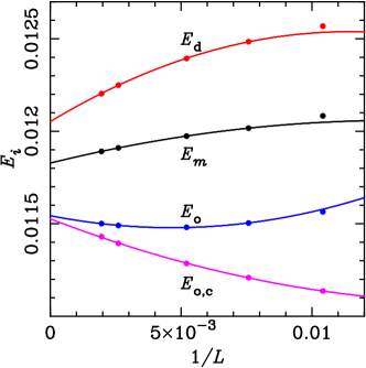
Figure 17: Estimates for the energies $E_{d}(L)$ (red), $E_{m}(L)$ (black) and $E_{o}(L)$ (blue) obtained from the histograms at $v_{\circ}(L)$ for $L\geq 96$. The data are displayed in Table 2, and the error bars are smaller than the size of the points. The curves correspond to the actual fits to the Ansatz (59). The pink points correspond to the estimates for $E_{o,c}(L)$ obtained from the histograms at $v=v_{c}$ (see Table 3), and the pink curve is the actual fit to those points (71).

The best results correspond to $L_{\text{min}}=132$ (DF = 1):

$$E_{o} \;=\;0.011\,544(5)\,,$$ (60a)

$$E_{d} \;=\;0.012\,052(5)\,,$$ (60b)

$$E_{m} \;=\;0.011\,828(9)\,.$$ (60c)

The values of $\chi^{2}$ are $0.70$, $2.46$, and $4.87\times 10^{-3}$, respectively. The corresponding confidence levels are 40.4%, 11.7%, and 94.4%.

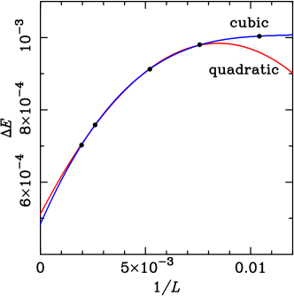
Figure 18: Estimates for the latent heat $\Delta E(L)$ obtained by using the histogram method for $L\geq 96$. The data are displayed in Table 2, and the error bars are smaller than the size of the points. The curve labeled “quadratic” corresponds to the Ansatz (59) and the results (61). The other curve labeled “cubic” corresponds to a cubic Ansatz and the results (62).

For the latent heat $\Delta E(L)$, we have first used the same Ansatz (59), and the best results correspond to $L_{\text{min}}=132$:

$$\Delta E\;=\;0.000\,511(6)\,,$$ (61)

with $\chi^{2}/\text{DF}=3.57/1$ and $\text{CL}=5.89\%$. This last value is rather poor, so we tried to add a cubic term $C/L^{3}$ to the Ansatz (59). In this case, we get a better fit for $L_{\text{min}}=96$:

$$\Delta E\;=\;0.000\,48(1)\,,$$ (62)

with $\chi^{2}/\text{DF}=0.22/1$ and $\text{CL}=66.6\%$. Both fits (61) and (62) are shown in Fig. 18.

It is clear from either the study of the position of the peaks $E_{o}$ and $E_{d}$ (60), or equivalently, from the study of the latent heat (61) and (62) that the transition is of first order. In the latter case, the estimates for the latent heat are many standard deviations away from $\Delta E=0$. Notice that the value of the latent heat (per edge) is two orders of magnitude smaller than the latent heat for the five-state square-lattice FM Potts model $\Delta E=0.026\,459\,378\ldots$ Baxter_73 , which is one canonical example of a very weak first-order phase transition.

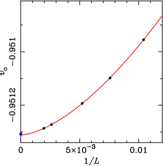
Figure 19: Estimate of the pseudocritical temperature $v_{\circ}(L)$ for $L\geq 96$ displayed in Table 1. The corresponding curve corresponds to the Ansatz (63). The blue point at $1/L=0$ is the MC estimate (41).

We have also fitted the quantity $v_{\circ}(L)$ displayed in Table 1 to a power-law Ansatz:

$$v_{\circ}(L)\;=\;v_{c}+L^{-\omega}\,.$$ (63)

The best result corresponds to $L_{\text{min}}=96$:

$$v_{c} \;=\;-0.951\,311\,0(7)\,,$$ (64a)

$$\omega \;=\;\phantom{-}1.60(1)\,,$$ (64b)

with $\chi^{2}/\text{DF}=1.06/2$, and $\text{CL}=58.9\%$ (see Fig. 19).

This result for $v_{c}$ is slightly smaller than the MC estimate $v_{c}=-0.951\,308(2)$ (41); but the difference is only $1.5$ standard deviations of the latter estimate. Notice that the exponent in (64) is expected to be $\omega=2$. This difference can be explained by the fact that our lattices are too small to attain the expected asymptotic behavior.

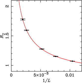
Figure 20: Estimates for the ratio $R_{2}(L)$ for $L\geq 96$ and displayed in Table 1. The curve corresponds to the Ansatz (65).

Let us now consider the ratio $R_{2}(L)$ (58). If this ratio grows as $L$ increases, it means that the value of $P_{m}(L)$ becomes exponentially small with respect to the values $P_{o}(L)=P_{d}(L)$. The data are displayed in Table 1. We have tried a power-law fit with a constant:

$$R_{2}(L)\;=\;A\,L^{\omega}+B\,.$$ (65)

We obtain a good fit for $L_{\text{min}}=96$:

$$\omega\;=\;0.65(3)\,,$$ (66)

with $\chi^{2}/\text{DF}=0.65/2$ and $\text{CL}=72.2\%$ (see Fig. 20).

Finally, we are going to consider the interface tension $\sigma_{od}(L)$. Notice that this study is usually performed at the bulk critical temperature by defining the estimate for a 2D system of linear size $L$ as Billoire_94 ; Billoire_95 :

$$2\sigma_{od}(L)\;=\;\frac{1}{L}\,\log(R_{2}(L))\,.$$ (67)

However this method has also been applied at the pseudocritical temperature $v_{\circ}(L)$, where the two peaks attain the same height Berg_93 . (See also the discussion in Ref. (Billoire_94, , end of Sec. 3).) The data are depicted in Fig. 21. The behavior of $2\sigma_{od}(L)$ is nonmonotonic with $L$, so we do not expect a very good fit due to the small number of data points we have. We have tried a quadratic fit in $1/L$:

$$2\sigma_{od}(L)\;=\;2\sigma_{od}+A/L+B/L^{2}\,.$$ (68)

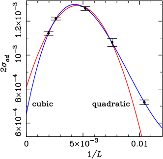
Figure 21: Estimates for the interface tension $2\sigma_{od}(L)$ (67) for $L\geq 96$ obtained from the ration $R_{2}(L)$ displayed in Table 1. The blue curve corresponds to the quadratic Ansatz (68). The red curve corresponds to a cubic Ansatz in $1/L$.

The best result corresponds to $L_{\text{min}}=132$:

$$2\sigma_{od}\;=\;0.000\,81(4)\,,$$ (69)

with $\chi^{2}/\text{DF}=2.08/1$ and $\text{CL}=14.9\%$. If we add a cubic term $C/L^{3}$ to the Ansatz (68), we find a good result for $L_{\text{min}}=96$:

$$2\sigma_{od}\;=\;0.000\,65(8)\,,$$ (70)

with $\chi^{2}/\text{DF}=0.059/1$ and $\text{CL}=80.7\%$.

For a first-order phase transition, we expect that $2\sigma_{od}(L)$ has a positive limit when $L\to\infty$. If the transition is second-order, this limit is expected to be zero. For the five-state FM Potts model on the square lattice, the interface surface is given by $\sigma_{od}=0.000\,398\,050\ldots$ Borgs_92b ; Janke_94 . This number is one order of magnitude smaller than the estimate we obtained using the growth of the autocorrelation time [c.f., (53)], but is of the same order of magnitude than the previous estimates (69) and (70). Therefore, even though our results are small, they are not consistent with zero, and there are well-known first-order phase transitions with interface tension this small.

In any case, our results (69) and (70) are consistent with a first-order phase transition; but the difference between both estimates indicate that we have not attained yet the asymptotic regime. Moreover, the exponent $\omega$ found for the growth of the ratio $R_{2}(L)$ (66) is not consistent with the expected result $\omega=1$ for a 2D system Billoire_94 . Again, these results should be interpreted with a grain of salt, as the linear sizes of the simulated systems are not large enough.

V.2 Analysis at the critical temperature

We have followed the same procedure to estimate the value of $E_{o}(L)$ from the histograms at $v=v_{c}$ (see Fig. 14). This is a consistency check for the procedure followed in the previous section. In this case, we have fitted the data close to the peak at $E_{o}(L)$, which in this case we have chosen to be in the interval $[P_{o}(L),P_{o}(L)/2]$. [Choosing $P_{o}(L)/e$ will lead to points too close to the incipient small bump at $E_{d}(L)$.] The mean value comes from the estimates obtained at $v_{c}=-0.951\,308(2)$ (41); and the error bars take into account the statistical errors, as well as the dispersion obtain by repeating the procedure at $v=-0.951\,306$ and $v_{c}=-0.951\,310$. The data are displayed in Table 3 and depicted in the lowermost curve of Fig. 17.

$L$	$E_{o}$
96	$0.011\,136(2)$
132	$0.011\,209(2)$
192	$0.011\,286(3)$
384	$0.011\,394(5)$
510	$0.011\,430(6)$

Table 3: For each value of $L=96,132,192,384,510$, we show the estimates for the position of the ordered peak $E_{o}(L)$ obtained from the histogram at $v=v_{c}$ (see the lower curve labeled “$E_{o,c}$” in Fig. 14).

We have used the quadratic Ansatz in $1/L$ (59), and we obtain a good result for $L_{\text{min}}=96$:

$$E_{o}\;=\;0.011\,527(8)\,,$$ (71)

with $\chi^{2}/\text{DF}=1.34/2$ and $\text{CL}=51.1\%$. This value differs from the previous estimate (60a) by $\sim 1.7\times 10^{-5}$, i.e., roughly two standard deviations given in (71).

Finally, we could find the position of the small “bump” displayed by the probability distribution for $L=510$ (see Fig. 14). Using this value, we could estimate the latent heat

$$\Delta E(510)\;=\;0.000\,708(6)\,,$$ (72)

which agrees well with the estimate obtained in the previous section (see Table 2).

V.3 Other physical quantities

It is well known Binder_84 ; Challa_86 ; Borgs_90 ; Borgs_91 ; Lee_91 ; Billoire_Lacaze_Morel_92 that the specific heat for a 2D system undergoing a first-order phase transition has a maximum value $C_{H,\text{max}}(L)$ at a point $v_{C_{H,\text{max}}}(L)$ such that

$$v_{C_{H,\text{max}}}(L) \;=\;v_{c}+A\,L^{-2}+\cdots\,,$$ (73a)

$$C_{H,\text{max}}(L) \;=\;A\,L^{2}+B+C\,L^{-2}+\cdots\,,$$ (73b)

where the dots represent higher-order powers in $L^{-2}$. Similar results are obtained for the minimum of the Binder cumulant $U_{4}$:

$$v_{U_{4,\text{min}}}(L) \;=\;v_{c}+A\,L^{-2}+\cdots\,,$$ (74a)

$$U_{4,\text{min}}(L) \;=\;A\,L^{2}+B+C\,L^{-2}+\cdots\,,$$ (74b)

$L$	$v_{C_{H,\text{max}}}$	$C_{H,\text{max}}$	$v_{U_{4,\text{min}}}$	$U_{4,\text{min}}$
96	$-0.950\,962(2)$	$0.094\,7(1)$	$-0.950\,961(3)$	$2.203(3)$
132	$-0.951\,101(1)$	$0.127\,8(2)$	$-0.951\,096(2)$	$2.104(3)$
192	$-0.951\,193\,4(7)$	$0.186\,7(2)$	$-0.951\,189\,7(9)$	$2.009(2)$
384	$-0.951\,271\,4(2)$	$0.404\,8(6)$	$-0.951\,270\,8(3)$	$1.831(2)$
510	$-0.951\,285\,7(2)$	$0.571(1)$	$-0.951\,284\,8(4)$	$1.775(3)$

Table 4: For each value of $L=96,132,192,384,510$, we show the estimates for the position of the maximum of the specific heat $v_{C_{H,\text{max}}}$, the value of such maximum $C_{H,\text{max}}$, the position of the minimum of the Binder cumulant $v_{U_{4,\text{min}}}$, and the value of such minimum $U_{4,\text{min}}$.

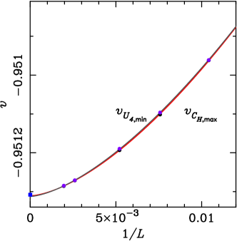
Figure 22: Estimates of the pseudocritical temperatures $v_{C_{H,\text{max}}}$ (black points) and $v_{U_{4,\text{min}}}$ (violet points) for $L\geq 96$ displayed in Table 4. The corresponding curves (that are almost indistinguishable) correspond to the Ansatz (75) for the latter (red curve), and (79) for the former (dark gray curve). The blue point at $1/L=0$ is the MC estimate (41).

By using the Ferrenberg–Swendsen extrapolation method, we have been able to locate these maxima of the specific heat for $L\geq 96$. We have used the same method as in Sec. V.1: (1) Obtain the mean values for $v_{C_{H,\text{max}}}(L),C_{H,\text{max}}(L)$ by using the whole set of measurements; and (2) in order to estimate the error bars, split this set of measurements into $N=20$ groups with identical size, compute estimates for these quantities within each group, and obtain its mean value and standard deviation assuming that the results coming from each group are statistically independent from the rest. These results are displayed in Table 4. We also performed a jackknife analysis of these data, but again the error bars were too small: e.g., for $L=192$, the jackknife estimate for the error bar is $\approx 10^{-5}$ (i.e., $20$ times smaller that the error quoted in Table 4). However, the value of the specific heat for the original MC simulation is $C_{H}(-0.95119;192)=0.187(2)$. This error bar is $10$ times the error quoted in Table 4 but $200$ times larger than the jackknife one. Therefore, we conclude that the latter errors are too small, and we prefer to consider the more conservative ones displayed in Table 4. In a similar way we have obtained the corresponding results for the mimima of $U_{4}(L)$.

Let us consider the values of $v_{C_{H,\text{max}}}(L)$. If we use the Ansatz [inspired by the exact result (73a)]:

$$v_{C_{H,\text{max}}}(L)\;=\;v_{c}+A\,L^{-\omega}\,,$$ (75)

we obtain a good fit for $L_{\text{min}}=132$:

$$v_{c} \;=\;-0.951\,312(1)\,,$$ (76a)

$$\omega \;=\;\phantom{-}1.54(3)\,,$$ (76b)

with $\chi^{2}/\text{DF}=0.32/1$, and $\text{CL}=57.0\%$. See the red curve in Fig. 22. These results are very similar to the ones we obtained for $v_{\circ}(L)$ [cf., (64)].

Similarly, we used the Ansatz

$$C_{H,\text{max}}(L)\;=\;A\,L^{\omega}+B\,,$$ (77)

which is inspired by the exact result (73b). The “best” result is obtained for $L_{\text{min}}=132$:

$$\omega\;=\;1.275(5)\,,$$ (78)

with $\chi^{2}/\text{DF}=5.97/1$, and $\text{CL}=1.45\%$. The confidence level is rather poor. The best explanation we have is that the sizes of our systems are still too small compared to the infinite-volume (finite) correlation length $\xi_{c}$ at $v=v_{c}$. Notice that $\omega=1.275(5)$ is compatible within errors with the estimate for $\alpha/\nu=1.21(7)$ (46) obtained in Sec. IV.3 from the standard FSS analysis of the MC data (see Fig. 23).

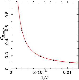
Figure 23: Estimates for the maximum value of the specific heat $C_{H,\text{max}}(L)$ as a function of $L\geq 96$. The data is displayed in Table 4. The curve corresponds to the Ansatz (77). Error bars are smaller than the symbols.

Let us now repeat the same analysis for the Binder cumulant $U_{4}$. If we consider the values of $v_{U_{4,\text{min}}}(L)$ and use the Ansatz

$$v_{U_{4,\text{min}}}(L)\;=\;v_{c}+A\,L^{-\omega}\,,$$ (79)

the “best” fit is obtained for for $L_{\text{min}}=96$:

$$v_{c} \;=\;-0.951\,313(1)\,,$$ (80a)

$$\omega \;=\;\phantom{-}1.53(2)\,,$$ (80b)

with $\chi^{2}/\text{DF}=4.67/2$, and $\text{CL}=9.68\%$. These results are very similar to the ones we obtained for (76), and to those for $v_{\circ}(L)$ [cf., (64)].

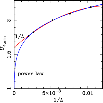
Figure 24: Estimates for the minimum value of the Binder cumulant $U_{4,\text{min}}(L)$ as a function of $L\geq 96$. The data are displayed in Table 4. The lower blue curve corresponds to the Ansatz (81), and the upper red curve to the Ansatz (83). Error bars are smaller than the symbols.

For the mimimum value of $U_{4}$, we first used the Ansatz

$$U_{4,\text{min}}(L)\;=\;U_{4,c}+B\,L^{-\omega}\,.$$ (81)

The “best” result is obtained for $L_{\text{min}}=96$:

$$U_{4,c} \;=\;0.7(2)\,,$$ (82a)

$$\omega \;=\;0.20(3)\,,$$ (82b)

with $\chi^{2}/\text{DF}=8.77/2$, and $\text{CL}=1.25\%$. The confidence level is rather poor. This is the blue curve on Fig. 24. One flaw of this result is that the value for $U_{4,c}<1$, which is impossible Billoire_Lacaze_Morel_92 : $U_{4,c}\geq 1$, and it attains the value $U_{4,c}=1$ when it is the sum of two delta functions. Therefore, we tried the following Ansatz:

$$U_{4,\text{min}}(L)\;=\;U_{4,c}+A\,L^{-1}+B\,L^{-2}\,,$$ (83)

as the behavior of $U_{4,\text{min}}(L)$ seems rather smooth as a function of $1/L$ on Fig. 24. The result in this case is

$$U_{4,c}\;=\;1.575(8)\,,$$ (84)

for $L_{\text{min}}=132$, $\chi^{2}/\text{DF}=9.02\times 10^{-8}/1$, and $\text{CL}=100\%$. This result corresponds to the red curve on Fig. 24. Probably the right value is somewhere in between these two values, as we have seen in other fits that the expected asymptotic regime has not been attained due to the fact that $L\ll\xi_{c}$.

VI Conclusions

In this paper we have performed a high-precision MC study of the five-state AF Potts model on the BH lattice. We have found that there is a low-$T$ phase where five distinct phases coexist (see Appendix B), and a standard paramagnetic disordered phase at high temperature. In between there is a phase transition at $v_{c}=-0.951\,308(2)$, which is one order of magnitude more precise than previous determinations union-jack .

The “standard” analysis of the MC data gives a value for the exponent $y_{t}=1/\nu=2.0(1)$, which is compatible within errors with the expected value for a first-order phase transition in a 2D system Nauenberg_74 ; Klein_76 ; Fisher_82 . However the values of the critical-exponent ratios are far from the expected ones: namely, $\alpha/\nu=1.21(2)$ and $\gamma/\nu=1.766(9)$. (The expected values of these ration is $2$ for a 2D system undergoing a first-order phase transition). Notice that there is a clear inconsistency between the values of $1/\nu=2.0(1)$ and $\alpha/\nu=1.21(2)$: below the upper critical dimension $D<4$, the “hyperscaling” relation for a $D$-dimensional system is expected to hold (see Ref. Pelissetto_02 , Sec. 1.3):

$$(2-\alpha)/\nu\;=\;D\,.$$ (85)

The lhs is $\approx 2.79$, while the rhs is equal to $D=2$.

Concerning the dynamics of the WSK algorithm, its slowest mode turns out to be the square magnetization $\bm{\mathcal{M}}^{2}$ (12). It is clear from the MC data (see Fig. 4) that the system suffers from critical slowing down: the autocorrelation times diverges close to the bulk critical point. If we assume that this divergence is like a power (as in second-order critical points Sokal_97 ), we obtain the dynamic critical exponent $z_{\text{int},\bm{\mathcal{M}}^{2}}=1.54(6)$. This is smaller than the expected value ($\gtrsim 2$) for single-site MC algorithms. On the other hand, if we assume the exponential growth $\tau_{\text{int},\bm{\mathcal{M}}^{2}}\sim\exp\bigl{(}\sigma_{od}\,L\bigr{)}$ which characterizes the behavior for a first-order phase transition on a 2D system, we find a very small interface tension $\sigma_{od}=0.0035(1)$.

It is worth noticing that the fits for the universal amplitudes $R$, $U_{4}$, and $\xi/L$ (see Figs. 7–9), even though they needed $L_{\text{min}}=192,384$, the curves for smaller values of $L$ were not too far from the corresponding data points. However, the fits for $C_{H}$, $\chi$, and $\tau_{\text{int},\bm{\mathcal{M}}^{2}}$ did need $L_{\text{min}}=384$, and the curves for smaller values of $L$ look quite far away from the corresponding points (especially for the dynamic data; see Figs. 10–13).

Due to the fact that some results were in good agreement with a first-order phase transition, while others pointed in the other direction, we analyzed the data using the histogram method. Even though one can get only some partial results from the energy histograms extrapolated to the bulk critical point $v_{c}$, the whole picture can be studied by considering these histograms extrapolated to a pseudocritical temperature $v_{\circ}(L)$ defined as the one such that the histogram has two peaks of equal height. Notice that this two-peak structure appears only for $L\gtrsim 96$, while it is absent for $L\lesssim 48$. The first result is that there is a tiny latent heat (per edge) for this system $\Delta E=0.000\,48(1)$ (and the position of the peak corresponding to the low-$T$ ordered phase $E_{o}$ was in good agreement with the estimate obtained from the histograms at $v_{c}$). We call it “tiny” because it is two orders of magnitude smaller than the latent heat for other weak first-order phase transitions Baxter_73 ; Adler_95 . From this result, we conclude that the transition is an extremely weak first-order one. Indeed, the extrapolation of the pseudocritical points $v_{\circ}(L)$ agrees well with the value obtained in the “standard” analysis of the MC data.

We could also estimate the interface tension $\sigma_{od}$ from these histograms extrapolated at $v_{\circ}(L)$. Its behavior with $1/L$ is not monotonic, and we do not have many data points. So the results are not very conclusive: $\sigma_{od}=0.000\,7(1)$. This value is five times smaller from the estimate obtained from the growth of the autocorrelation time $\tau_{\text{int},\bm{\mathcal{M}}^{2}}$ (see Fig. 21).

Finally, we also considered the position of the maximum of the specific heat and the minimum of $U_{4}$, leading to new pseudocritical temperatures $v_{C_{H,\text{max}}}$ and $v_{U_{4,\text{min}}}$, respectively (see Fig. 22). Their behavior is very similar to that of $v_{\circ}(L)$, and the extrapolated values are close to the bulk critical point $v_{c}$, although in general the estimates coming from the histogram method are slightly smaller than that coming from the standard MC analysis [e.g., $-0.951\,311(2)$ versus $-0.951\,308(2)$]. We also tried to analyze how the maximum of the specific heat $C_{H,\text{max}}$ and the minimum of the Binder cumulant $U_{4,\text{min}}$ behave with $L$. Notice that the confidence levels for the power-law fits to these quantities are rather poor (see Figs. 23 and 24).

The result that the transition is an extremely weak first order implies that the correlation length at the bulk critical point is very large, but finite. For instance, for the five-state FM Potts model on the square lattice, we have that Borgs_92b ; Janke_94

$$\sigma_{od}\;\approx\;3.981\times 10^{-4}\,,\quad\xi_{d}\;=\;\frac{1}{\sigma_{od}}\;\approx\;2.512\times 10^{3}\,,$$ (86)

where $\xi_{d}$ is the critical correlation length on the disordered phase. Even though these figures do not correspond to our system, they can give us an order of magnitude. For instance, the interface tension is of the same order as the one obtained from the histogram method. The fact that $\xi_{d}\sim 10^{3}$ implies that the linear size of our systems are fairly small to “see” the correct scaling for a first-order transition. This is probably the reason why we do not get the expected values for $\gamma/\nu$ and $\alpha/\nu$, and the estimates for the interface tension do not agree among them.

For future work, the main problem left is to find a lattice $\mathcal{G}$ such that the five-state $\mathcal{G}$-lattice AF Potts model is critical. With respect to the five-state BH-lattice AF Potts model, there are two interesting technical problems to be solved: (1) Find the height representation for this model at $T=0$. As it is not disordered at all temperatures, it should have one such representation, as claimed by Henley Henley_unpub . (2) Even though the numerical data support the idea that WSK is ergodic for this lattice at $T=0$, we need a rigorous proof of such a claim. This would be a step towards proving the ergodicity of the WSK algorithm for the five-state AF Potts model on the triangular lattice.

Appendix A The right staggering

In this Appendix we will discuss the choice we have made for the staggering. If $q=3$, then the ‘obvious’ staggering would be to choose $\phi_{A}=0$, $\phi_{B}=2\pi/3$, and $\phi_{C}=-2\pi/3$. This choice is motivated by the fact that at $T=0$, the BH graph has a unique 3-coloring modulo global permutations of colors. Moreover, for $q=4$ and $T=0$, previous studies union-jack indicate that sublattice $A$ (the one with the largest-degree vertices) is ordered, while the other two sublattices are disordered. For $q=5$, one would expect naively similar behavior.

One way to find the right staggering is the following. We first define the magnetization density $\bm{\mathcal{M}}_{k}$ [cf., (9) and (10)] for each sublattice $k\in\{A,B,C\}$ as

$$\bm{\mathcal{M}}_{k}\;=\;\frac{1}{|V_{k}|}\,\sum\limits_{\bm{x}\in V_{k}}\bm{\sigma}_{\bm{x}}\,.$$ (87)

We now define the mean value of the product of two of such magnetizations densities

$$M_{ab} \;=\;\left\langle\bm{\mathcal{M}}_{a}\cdot\bm{\mathcal{M}}_{b}\right\rangle$$ (88a)

$$\;=\;\frac{q}{q-1}\frac{1}{|V_{a}|\,|V_{b}|}\sum\limits_{\alpha=1}^{q}\left\langle\sum\limits_{x\in V_{a}}\delta_{\sigma_{x},\alpha}\sum\limits_{y\in V_{b}}\delta_{\sigma_{y},\alpha}\right\rangle\qquad$$

$$\qquad\qquad-\frac{1}{q-1}\,,$$ (88b)

so that each diagonal entry is bounded in the interval $[0,1]$, while the nondiagonal ones are bounded in the interval $\bigl{[}-\frac{1}{q-1},1\bigr{]}$. In terms of these element, we can compute the mean square magnetization density quadratic form $\mathsf{M}=(M_{ab})_{a,b\in\{A,B,C\}}$

$$\mathsf{M}\;=\;\left(\begin{array}[]{ccc}M_{AA}&M_{AB}&M_{AC}\\ M_{AB}&M_{BB}&M_{BC}\\ M_{AC}&M_{BC}&M_{CC}\\ \end{array}\right)\,,$$ (89)

where we have used the obvious symmetry $M_{ab}=M_{ba}$.

We can now compute the eigenvalues and eigenvectors of (89). The eigenvector associated to the largest eigenvalue will correspond to the right staggering. As $\mathsf{M}$ is a real and symmetric matrix, its eigenvalues are real and the corresponding eigenvectors have real entries and can be chosen to form an orthogonal basis of ${\mathbb{R}}^{3}$.

Given the quadratic form (89), we can compute the susceptibility associated to any linear combination of the sublattice magnetizations (87). In particular, if the leading eigenvalue of (89) $\lambda_{\circ}$, and its associated eigenvector is $\bm{\alpha}_{\circ}=(\alpha_{A},\alpha_{B},\alpha_{C})\in{\mathbb{R}}^{3}$, then the linear combination

$$\bm{\mathcal{M}}_{\circ}\;=\;\sum_{a\in\{A,B,C\}}\alpha_{a}\,\bm{\mathcal{M}}_{a}$$ (90)

gives the susceptibility

$$\chi_{\circ}\;=\;|V_{\text{BH}}|\,\langle\bm{\mathcal{M}}_{\circ}\cdot\bm{\mathcal{M}}_{\circ}\rangle\;=\;|V_{\text{BH}}|\,\bm{\alpha}^{t}_{\circ}\cdot\mathsf{M}\cdot\bm{\alpha}_{\circ}\,.$$ (91)

Note that the normalization is distinct from that of Eq. (22a).

As a check, we can compute the staggering for the zero-temperature three-state AF Potts model on a triangular lattice of size $L\times L$. In this case, $M_{aa}=1$, and $M_{ab}=-1/2$ whenever $a\neq b$. The dominant eigenvalue of the quadratic form (89) is $\lambda_{\circ}=3/2$, and its associated eigenvector is $\bm{\alpha}_{\circ}=(1,-1,0)^{t}$. Then $\langle\bm{\alpha}^{t}_{\circ}\cdot\mathsf{M}\cdot\bm{\alpha}_{\circ}\rangle=3/2$. Notice that the standard staggering $\bm{\alpha}_{\text{st}}=\bigl{(}1,e^{2\pi i/3},e^{-2\pi i/3}\bigr{)}^{t}$ gives exactly the same result: $\left\langle\bm{\mathcal{M}}_{\text{st}}^{*}\cdot\bm{\mathcal{M}}_{\text{st}}\right\rangle=\left\langle(\bm{\alpha}^{*}_{\text{st}})^{t}\cdot\mathsf{M}\cdot\bm{\alpha}_{\text{st}}\right\rangle=3/2$.

Going back to the five-state BH-lattice AF Potts model, we focused in the interval $v\in[-0.952,-0.951]$. For each value of $L=24,48,96$, we performed $11$ MC simulations at equidistant values of $v$ in that interval. For each one of these runs, we discarded at least $10^{4}\,\tau_{\text{int}}$ MCS, and we took at least $9.5\times 10^{4}\,\tau_{\text{int}}$ measures.

$L$	$\alpha_{A}$	$\alpha_{B}$	$\alpha_{C}$
24	$0.92704$	$-0.28027$	$-0.24911$
48	$0.92674$	$-0.28117$	$-0.24919$
96	$0.92654$	$-0.28181$	$-0.24923$
Best	$0.927$	$-0.282$	$-0.249$

Table 5: For each value of $L=24,48,96$ and for $v=-0.9513$, we display the three components $\alpha_{i}$ of the (unitary) leading eigenvector $\bm{\alpha}_{\circ}$ of the quadractic form (89). The lower row (labeled “Best”) shows our preferred estimates for $\alpha_{i}$.

We computed the leading eigenvector $\bm{\alpha}_{\circ}$ of the quadratic form (89) for each simulation, and we saw that they behaved smoothly as a function of $v$. In order to determine the optimal value of $\bm{\alpha}_{\circ}$, we choose $v=-0.9513$, which is the one closest to the previous estimate of $v_{c}=-0.95132(2)$ union-jack . The numerical results are displayed in Table 5.

The results look rather stable as a function of $L$. As $\alpha_{A}/4\approx|\alpha_{B}|,|\alpha_{C}|$, we could define the staggered magnetization as this simple linear combination:

$$\bm{\mathcal{M}}_{\circ}\;=\;4\bm{\mathcal{M}}_{A}-\bm{\mathcal{M}}_{B}-\bm{\mathcal{M}}_{C}\,.$$ (92)

It is clear that the most relevant contribution to $\bm{\mathcal{M}}_{\circ}$ corresponds to $\bm{\mathcal{M}}_{A}$ (i.e., the sublattice with vertices of largest degree, in agreement with previous works union-jack ). Actually, what we need is an observable with a large overlap with $\bm{\mathcal{M}}_{\circ}$ (92). The simplest choice is

$$\bm{\mathcal{M}}_{\circ}\;=\;\bm{\mathcal{M}}_{A}\,.$$ (93)

This definition, although is not the optimal one, is expected to pick up the relevant physics of the system without the technical programming difficulties of using (92), and moreover, it is expected to reduce significantly the CPU time of the MC simulations. In the main text, we drop for notational simplicity the subindex $\circ$.

Appendix B The ground-state structure

Let us consider the five-state BH-lattice Potts model at $T=0$, and assume that WSK is ergodic for the graphs $G_{\text{BH},L}$ (see the discussion in Sec. III.2, in particular, Fig. 4). In this Appendix, we are going to consider first the six sublattices shown in Fig. 3 labeled 1 to 6, so that $A=\{1\}$, $B=\{2,3\}$, and $C=\{4,5,6\}$.

We have computed the corresponding enlarged mean square magnetization density quadratic form $\mathsf{M}=(M_{ab})_{a,b\in\{1,2,\ldots,6\}}$ [cf., (88) and (89)]. For the lattice with $L=96$, we performed $8\times 10^{6}$ MCS, discarded $\gtrsim 2.5\times 10^{4}\,\tau_{\text{int}}$, and took $\gtrsim 2.2\times 10^{5}\,\tau_{\text{int}}$ measurement. In this case, the slowest mode corresponded to $\mathcal{M}_{1}^{2}$. First, we checked that the obvious symmetries hold:

$$\mathsf{M}_{bb} \;=\;\phantom{-}0.062\,344\,0(3)\,,\quad b\in B\,,$$ (94a)

$$\mathsf{M}_{cc} \;=\;\phantom{-}0.060\,789\,1(9)\,,\quad c\in C\,,$$ (94b)

$$\mathsf{M}_{1b} \;=\;-0.235\,129(3)\,,\quad b\in B\,,$$ (94c)

$$\mathsf{M}_{1c} \;=\;-0.232\,186(4)\,,\quad c\in C\,,$$ (94d)

$$\mathsf{M}_{bc} \;=\;\phantom{-}0.061\,404\,5(6)\,,\quad b\in B\,,\quad c\in C\,,$$ (94e)

$$\mathsf{M}_{cd} \;=\;\phantom{-}0.060\,709\,7(8)\,,\quad c,b\in C\,\quad c\neq d\,.$$ (94f)

The numerical estimates come from fits to a constant Ansatz. In each fit, the data points are not statistically independent, so we have quoted for each quantity, instead of the error bar obtained from the fit, the more conservative error bar of the individual values (which were approximately constant). In all fits, there is at least one DF, and we obtain an excellent value for $\chi^{2}\lesssim 0.3$.

$L$	$\mathsf{M}_{AA}$	$\mathsf{M}_{BB}$	$\mathsf{M}_{CC}$
3	$\phantom{1}0.909(3)$	$\phantom{1}0.1458(3)$	$\phantom{1}0.1178(2)$
6	$\phantom{1}0.8944(9)$	$\phantom{1}0.08327(6)$	$\phantom{1}0.07510(4)$
12	$\phantom{1}0.8900(3)$	$\phantom{1}0.06746(1)$	$\phantom{1}0.06427(1)$
24	$\phantom{1}0.8886(1)$	$\phantom{1}0.063536(2)$	$\phantom{1}0.061577(5)$
48	$\phantom{1}0.88855(5)$	$\phantom{1}0.0625549(7)$	$\phantom{1}0.060906(2)$
96	$\phantom{1}0.88843(2)$	$\phantom{1}0.0623084(3)$	$\phantom{1}0.0607362(8)$
$\infty$	$\phantom{1}0.88841(2)$	$\phantom{1}0.0622266(3)$	$\phantom{1}0.0606800(8)$
$L_{\text{min}}$	$\phantom{1}6$	$12$	$\phantom{1}6$
$\chi^{2}/$DF	$\phantom{1}2.84/3$	$\phantom{1}1.97/2$	$\phantom{1}1.37/3$
CL	$41.7\%$	$37.4\%$	$71.2\%$

Table 6: Values of the diagonal terms of the quadratic form (89) as a function of $L$. The row labeled “$\infty$” shows the results obtained by fitting the data to a biased power-law Ansatz. We also display the values of $L_{\text{min}}$, $\chi^{2}/\text{DF}$, and CL of our preferred fit (see text).

Next, we computed the quadratic form (89) at $v=-1$, taking into account all these symmetries to improve the statistics. We simulate systems with $L=3,6,12,24,48,96$, and for each of them, we simulate $10^{6}-8\times 10^{7}$ MCS, discarded at least $3.1\times 10^{3}\tau_{\text{int}}$ MCS, and took $2.8\times 10^{4}\tau_{\text{int}}$ measures. For $L\geq 24$, we increased the statistics to at least $1.1\times 10^{5}\tau_{\text{int}}$ measures. The slowest mode corresponded to $\bm{\mathcal{M}}_{A}^{2}$. The diagonal terms of the quadratic form (89) for different values of $L$ are given in Table 6. For each diagonal element $\mathsf{M}_{aa}$ (with $a\in\{A,B,C\}$), we have performed a power-law fit $\mathsf{M}_{aa}(L)=\mathsf{M}_{aa}^{*}+B_{a}\,L^{-\omega_{a}}$. In all cases, we found values of $\omega_{a}$ that agree with $\omega_{a}=2$ within errors: namely, $\omega_{A}=2.0(2)$, $\omega_{B}=1.997(3)$, and $\omega_{C}=2.003(4)$. Therefore, we have performed biased power-law fits with $\omega_{a}=2$. The values of $\mathsf{M}_{aa}^{*}$ coming from these biased fits are displayed in Table 6 on the row labeled “$\infty$”. We also show the values of $L_{\text{min}}$, $\chi^{2}/\text{DF}$, and CL of our preferred fits.

The diagonal term $\mathsf{M}_{aa}$ of the quadratic form (89) measures the FM order of the spins within the sublattice $a\in\{A,B,C\}$. The study of these values provides some insight on the ground-state structure of our model, as shown previously in the literature selfdual1 ; selfdual2 . In particular, if the spins in sublattice $a$ are fully FM ordered, then $\mathsf{M}_{aa}=1$. Moreover, if the spins in this sublattice take $r=2,3,4,5$ values at random, then the corresponding values of $\mathsf{M}_{aa}$ are $3/8=0.375$, $1/6\approx 0.16667$, $1/16=0.0625$, and $0$, respectively. The last case corresponds to the spins in sublattice $a$ being completely uncorrelated.

Looking at Table 6, we see that $\mathsf{M}_{AA}=0.88841(3)$. This value is close to $1$, and more than twice $3/8$. We conclude that the degree-12 sublattice $A$ is almost (but not completely) FM ordered. On the other hand, the other two diagonal entries satisfy $\mathsf{M}_{CC}=0.0606800(8)\lesssim\mathsf{M}_{BB}=0.0622266(3)\lesssim 1/16=0.0625$. This means that the spins in the degree-6 sublattice $B$ take very approximately four distinct values at random, while those in the degree-4 sublattice $C$ are slightly more disordered.

These results coincide qualitatively with those presented in Refs. selfdual1 ; selfdual2 for several quadrangulations and $q=3$: the sublattice with vertices of largest degree is the most FM ordered, and the ordering of the other two sublattices is roughly that of having $q-1$ spin values at random. For these two lattices, the one with smaller degree is less ordered.

The results for the three-state AF Potts models presented in Refs. selfdual1 ; selfdual2 could be understood from a theoretical point of view: the zero-temperature 3-state AF Potts model on any plane quadrangulation has a “height” representation Henley_unpub ; Kondev_96 ; Burton_Henley_97 ; SS_98 ; Jacobsen_09 . Once the height mapping is known, the next step is to find the so-called ideal states: i.e., families of ground-state configurations whose corresponding height configurations are macroscopically flat, and maximize the entropy density. The long-distance behavior of this microscopic height model is expected to be controlled by an effective Gaussian model, which can be in two distinct phases. If the Gaussian model is in its rough phase (or at the roughening transition), then the spin model is critical at $T=0$. On the other hand, if the Gaussian model is in its smooth phase, then the corresponding spin model can be described by small fluctuations around the ideal states. In this case, the model exhibits long-range order at $T=0$. Roughly speaking, the ground state is ordered with with as many ordered and coexisting phases as the number of ideal states previously found.

In the five-state BH-lattice AF Potts model, we have found that sublattice $A$ is almost FM ordered, while the spins in the other two sublattices take the other four values randomly. As the spin configurations at $T=0$ should have zero energy (i.e., it should be a proper 5-coloring of the BH graph), there are many constraints that make the values of $\mathsf{M}_{aa}$ slightly different from the expected values $1$ and $1/16$, respectively. Therefore, there are five possible families of ground-state configurations, one for each value taken by the spins on sublattice A. This behavior is qualitatively the same as the one found in Refs. selfdual1 ; selfdual2 for three-state models (see also Ref. planar_AF_largeq for four-state models).

We can therefore describe the ground-state structure of our model as five coexisting ordered phases. Although we are not aware of any height representation for this particular model, we conjecture its existence based on the fact that $5<q_{c}(\text{BH})$, and on a conjecture due to Henley Henley_unpub claiming that any AF Potts model that does not admit a height representation at $T=0$ should be disordered at all temperatures $T\geq 0$.

To summarize, the low-temperature phase of the five-state BH-lattice AF Potts model can be well described by five coexisting ordered phases. As there is obviously a high-temperature disordered phase, there should be a finite-$T$ phase-transition point $v_{c}$. However, we cannot predict from the above discussion its nature. Finally, if this picture is correct, then the ground-state structure of the five-state BH-lattice AF Potts model is identical to that of the corresponding FM model, so they should belong to the same universality class. By using universality (Fisher_98, ; Pelissetto_02, , and references therein) arguments in the FM model, we conclude that the transition in both models should be of first order for any $q>4$ Baxter_73 ; Baxter_book .

- (1) R.B. Potts, Proc. Cambridge Philos. Soc. 48, 106 (1952).
- (2) F.Y. Wu, Rev. Mod. Phys. 54, 235 (1982); 55, 315 (E) (1983).
- (3) R.J. Baxter, Exactly Solved Models in Statistical Mechanics (Academic Press, New York, 1982).
- (4) F.Y. Wu, J. Appl. Phys. 55, 2421 (1984).
- (5) R.J. Baxter, J. Phys. C 6, L445 (1973).
- (6) R.J. Baxter, Proc. R. Soc. Lond. A 383, 43 (1982).
- (7) M.E. Fisher, Rev. Mod. Phys. 70, 653 (1998).
- (8) B. Nienhuis, J. Stat. Phys. 34, 731 (1984).
- (9) P. Di Francesco, P. Mathieu and D. Sénéchal, Conformal Field Theory (Springer-Verlag, New York, 1997).
- (10) J.T. Chalker, P.C.W. Holdsworth and E.F. Shender, Phys. Rev. Lett. 68, 855 (1992).
- (11) D. Welsh and C. Merino, J. Math. Phys. 41, 1127 (2000).
- (12) A.D. Sokal, Physica A 279, 324 (2000), arXiv:cond-mat/9910503.
- (13) J.A. Ellis-Monaghan and I. Moffatt, editors, Handbook of the Tutte Polynomial, Chapman & Hall/CRC Monographs and Research Notes in Mathematics (Apple Academic Press, Oakville, Canada, 2020).
- (14) J.L. Jacobsen and J. Salas, J. Combin. Theory B 103, 532 (2013), arXiv:1009.4062.
- (15) J.L. Jacobsen, J. Salas, and A.D. Sokal, J. Stat. Phys. 119, 1153 (2005), arXiv:cond-mat/0401026.
- (16) J. Salas and A.D. Sokal, J. Stat. Phys. 86, 551 (1997), arXiv:cond-mat/9603068.
- (17) A. Sutö, Helv. Phys. Acta 54, 191 (1981).
- (18) A. Sutö, Z. Phys. B 44, 121 (1981).
- (19) J. Stephenson, J. Math. Phys. 5, 1009 (1964).
- (20) J. Adler, A. Brandt, W. Janke, and S. Shmulyian, J. Phys. A 28, 5117 (1995).
- (21) R. Kotecký, J. Salas, and A.D. Sokal, Phys. Rev. Lett. 101, 030601 (2008), arXiv:0802.2270.
- (22) P.W. Kasteleyn and C.M. Fortuin, J. Phys. Soc. Japan, 26 (Suppl.), 11 (1969).
- (23) C.M. Fortuin and P.W. Kasteleyn, Physica 57, 536 (1972).
- (24) J.L. Jacobsen and J. Salas, unpublished (2008).
- (25) Y. Deng, Y. Huang, J.L.Jacobsen, J. Salas, and A.D. Sokal, Phys. Rev. Lett. 107, 150601 (2011), arXiv:1108.1743.
- (26) Y. Huang, K. Chen, Y. Deng, J.L.Jacobsen, R. Kotecký, J. Salas, A.D. Sokal, and J.M. Swart, Phys. Rev. E 87, 012136 (2013), arXiv:1210.6248.
- (27) H. Saleur, Commun. Math. Phys. 132, 657 (1990).
- (28) H. Saleur, Nucl. Phys. B 360, 219 (1991).
- (29) J. Salas and A.D. Sokal, J. Stat. Phys 104, 609 (2001), arXiv:cond-mat/0004330.
- (30) J.L. Jacobsen and J. Salas, J. Stat. Phys 104, 701 (2001), arXiv:cond-mat/0011456.
- (31) J.L. Jacobsen, J. Salas, and A.D. Sokal, J. Stat. Phys. 112, 921 (2003), arXiv:cond-mat/0204587.
- (32) J.L. Jacobsen and J. Salas, J. Stat. Phys. 122, 705 (2006), arXiv:cond-mat/0407444.
- (33) J.L. Jacobsen and J. Salas, Nucl. Phys. B 783, 238 (2007), arXiv:cond-mat/0703228.
- (34) J. Salas and A.D. Sokal, J. Stat. Phys 135, 279 (2009), arXiv:0711.1738.
- (35) J. Salas and A.D. Sokal, J. Stat. Phys 144, 1028 (2011), arXiv:1002.3761.
- (36) J.L. Jacobsen, J. Salas and C.R. Scullard, J. Phys. A 50, 345002 (2017), arXiv:1702.02006.
- (37) R.J. Baxter, J. Phys. A 19, 2821 (1986).
- (38) R.J. Baxter, J. Phys. A 20, 5241 (1987).
- (39) J.L. Jacobsen and C.R. Scullard, J. Phys. A 45, 494003 (2012), arXiv:1204.0622
- (40) C.R. Scullard and J.L. Jacobsen, J. Phys. A 45, 494004 (2012), arXiv:1209.1451;
- (41) J.L. Jacobsen and C.R. Scullard, J. Phys. A 46, 075001 (2013), arXiv:1211.4335;
- (42) J.L. Jacobsen, J. Phys. A 47, 135001 (2014) arXiv:1401.7847.
- (43) C.R. Scullard and J.L. Jacobsen, J. Phys. A 49, 125003 (2016), arXiv:1511.04374.
- (44) E. Vernier, J.L. Jacobsen and J. Salas, J. Phys. A 49, 174004 (2016), arXiv:1509.02804.
- (45) J.-P. Lv, Y. Deng, J.L. Jacobsen, J. Salas, and A.D. Sokal, Phys. Rev. E 97, 040104(R) (2018), arXiv:1712.07047.
- (46) J.-P. Lv, Y. Deng, J.L. Jacobsen, and J. Salas, J. Phys. A 51, 365001 (2018), arXiv:1804.08911.
- (47) G. Delfino and E. Tartaglia, Phys. Rev. E 96, 042137 (2017), arXiv:1707.00998.
- (48) D.P. Landau and K. Binder, A Guide to Monte-Carlo Simulations in Statistical Physics, 3rd ed. (Cambridge University Press, Cambridge, 2009).
- (49) N. Madras, Lectures on Monte Carlo Methods, Fields Institute Monographs (AMS, Providence, RI, 2002).
- (50) M. Nauenberg and B. Nienhuis, Phys. Rev. Lett. 33, 944 (1974).
- (51) W. Klein, D.J. Wallace, and P.K.P. Zia, Phys. Rev. Lett. 37, 639 (1976).
- (52) M.E. Fisher and A.N. Berker, Phys. Rev. B 26, 2507 (1982).
- (53) J.-S. Wang, R.H. Swendsen, and R. Kotecký, Phys. Rev. Lett. 63, 109 (1989)
- (54) J.-S. Wang, R.H. Swendsen, and R. Kotecký, Phys. Rev. B 42, 2465 (1990).
- (55) M. Aizenman and E.H. Lieb, , J. Stat. Phys. 24, 279 (1981).
- (56) Y. Chow and F.Y. Wu, Phys. Rev. B 36, 285 (1987).
- (57) C.L. Henley, Discrete spin models with “height” representations and critical ground states, unpublished manuscript (September, 1993).
- (58) J. Kondev and C.L. Henley, Nucl. Phys. B 464, 540 (1996), arXiv:cond-mat/9511102.
- (59) J.K. Burton Jr. and C.L. Henley, J. Phys. A 30, 8385 (1997), arXiv:cond-mat/9708171.
- (60) J. Salas and A.D. Sokal, J. Stat. Phys 92, 729 (1998), arXiv:cond-mat/9801079.
- (61) J.L. Jacobsen, in Polygons, Polyominoes and Polycubes, edited by A.J. Guttmann, Lecture Notes in Physics, vol. 775 (Springer, Dordrecht, 2009), pp. 347–424.
- (62) V. Privman, editor, Finite Size Scaling and Numerical Simulation of Statistical Systems (Word Scientific, Singapore, 1990).
- (63) N. Madras and A.D. Sokal, J. Stat. Phys. 50, 109 (1988).
- (64) A.D. Sokal, in Functional Integration: Basics and Applications (1996 Cargèse summer school), edited by C. DeWitt-Morette, P. Cartier, and A. Folacci. (Plenum, New York, 1997), pp. 131–192.
- (65) J. Lee and J.M. Kosterlitz, Phys. Rev. B 43, 3265 (1991).
- (66) A.M. Ferrenberg and R.H. Swendsen, Phys. Rev. Lett. 61, 2635 (1988).
- (67) M. Weigel and W. Janke, Phys. Rev. E 81, 066701 (2010), arXiv:1002.4517.
- (68) P. Young, Everything you wanted to know about data analysis and fitting but were afraid to ask, arXiv:1210.3781 (2012).
- (69) C. Borgs and R. Kotecký, J. Stat. Phys. 61, 79 (1990).
- (70) C. Borgs, R. Kotecký, and S. Miracle-Solé, J. Stat. Phys. 62, 529 (1991).
- (71) K. Binder and D.P. Landau, Phys. Rev. B 30 1477 (1984).
- (72) M.S.S. Challa, D.P. Landau, and K. Binder, Phys. Rev. B 34 1841 (1986).
- (73) B. Grünbaum and G.C. Shephard, Tilings and Patterns (W.H. Freeman and Co., New York, 1987).
- (74) A. Billoire, R. Lacaze, and A. Morel, Nucl. Phys. B 370, 773 (1992).
- (75) S.-H. Tsai and S.R. Salinas, Braz. J. Phys. 28, 58 (1998), arXiv:cond-mat/9810412.
- (76) J. Salas and A.D. Sokal, J. Stat. Phys 98, 551 (2000), arXiv:cond-mat/9904038.
- (77) B. Mohar, Kempe equivalence of colorings, in Graph Theory in Paris, edited by J.A. Bondy, J. Fonlupt, J.L. Fouquet, J.-C. Fournier and J. Ramírez Alfonsín (Birkhäuser, Basel, 2007), pp. 287–297.
- (78) S.J. Ferreira and A.D. Sokal, J. Stat. Phys. 96, 461 (1999), arXiv:cond-mat/9811345.
- (79) R.H. Swendsen and J.-S. Wang, Phys. Rev. Lett. 58, 86 (1987).
- (80) J. Salas and A.D. Sokal, J. Stat. Phys. 87, 1 (1997), arXiv:hep-lat/9605018.
- (81) T.M. Garoni, G. Ossola, M. Polin, and A.D. Sokal, J. Stat. Phys. 144, 459 (2011), arXiv:1105.0373.
- (82) J. Salas, J. Phys. A 31, 5969 (1998), arXiv:cond-mat/9802145.
- (83) B. Mohar and J. Salas, J. Phys. A 42, 225204 (2009), arXiv:0901.1010.
- (84) B. Mohar and J. Salas, J. Stat. Mech. P05016 (2010), arXiv:1002.4279.
- (85) M. Lubin and A.D. Sokal, Phys. Rev. Lett. 71, 1778 (1993).
- (86) M. Jerrum, private communication.
- (87) J. McDonald, B. Mohar, and D. Scheide, J. Graph Theory 70, 226 (2012), arXiv:1005.2248.
- (88) M. Bonamy, N. Bousquet, C. Feghali, and M. Johnson, J. Combin. Theory B 135, 179 (2019), arXiv:1510.06964.
- (89) J. Salas and A.D. Sokal, unpublished (1998).
- (90) G. Ossola and A.D. Sokal, Phys. Rev. E 70, 027701 (2004), arXiv:hep-lat/0403010.
- (91) G. Ossola and A.D. Sokal, Nucl. Phys. B 691, 259 (2004), arXiv:hep-lat/0402019.
- (92) A. Billoire, T. Neuhaus, and B. Berg, Nucl. Phys. B 413 795 (1994), arXiv:hep-lat/9307017.
- (93) R. Kotecký, A.D. Sokal, and J.M. Swart, Commun. Math. Phys. 330, 1339 (2014), arXiv:1205.4472.
- (94) J. Lee and J.M. Kosterlitz, Phys. Rev. Lett. 65, 137 (1990).
- (95) C. Borgs and W. Janke, Phys. Rev. Lett. 68, 1738 (1992).
- (96) W. Janke, Phys. Rev. B 47, 14757 (1993).
- (97) W. Janke, Recent Developments in Monte-Carlo Simulations of First-Order Phase Transitions, in Computer Simulation Studies in Condensed-Matter Physics VII, edited by D.P. Landau, K.K. Mon, and H.-B. Schüttler (Springer-Verlag, Berlin, 1994), pp. 29–43, arXiv:hep-lat/9410021.
- (98) A. Billoire, Nucl. Phys. B (Proc. Suppl.) 42 21 (1995), arXiv:hep-lat/9501003.
- (99) B.A. Berg and T. Neuhaus, Phys. Rev. Lett. 68, 9 (1992), arXiv:hep-lat/9202004.
- (100) C. Borgs and W. Janke, J. Phys. I France 2, 2011 (1992).
- (101) A. Pelissetto and E. Vicari, Phys. Rep. 368, 549 (2002), arXiv:cond-mat/0012164.