BRITE-Constellation photometry of $\mn@boldsymbol{\pi}^{5}$ Orionis, an ellipsoidal SPB variable

Abstract

Results of an analysis of the BRITE-Constellation photometry of the SB1 system and ellipsoidal variable $\pi^{5}$ Ori (B2 III) are presented. In addition to the orbital light-variation, which can be represented as a five-term Fourier cosine series with the frequencies $f_{\rm orb}$, $2f_{\rm orb}$, $3f_{\rm orb}$, $4f_{\rm orb}$ and $6f_{\rm orb}$, where $f_{\rm orb}$ is the system’s orbital frequency, the star shows five low-amplitude but highly-significant sinusoidal variations with frequencies $f_{i}$ ($i={}$2,..,5,7) in the range from 0.16 to 0.92 d^-1. With an accuracy better than 1$\sigma$, the latter frequencies obey the following relations: $f_{2}-f_{4}=2f_{\rm orb}$, $f_{7}-f_{3}=2f_{\rm orb}$, $f_{5}=f_{3}-f_{4}=f_{7}-f_{2}$. We interpret the first two relations as evidence that two high-order $\ell=1,m=0$ gravity modes are self-excited in the system’s tidally distorted primary component. The star is thus an ellipsoidal SPB variable. The last relations arise from the existence of the first-order differential combination term between the two modes. Fundamental parameters, derived from photometric data in the literature and the Hipparcos parallax, indicate that the primary component is close to the terminal stages of its main sequence (MS) evolution. Extensive Wilson-Devinney modeling leads to the conclusion that best fits of the theoretical to observed light-curves are obtained for the effective temperature and mass consistent with the primary’s position in the HR diagram and suggests that the secondary is in an early MS evolutionary stage.

1 Introduction

The radial velocity (RV) of $\pi^{5}$ Ori (HD 31237, HR 1567, HIP 22797) was discovered to be variable with a range of about 110 km s^-1 by Frost & Adams (1903). Lee (1913) found the star to be a single-lined spectroscopic binary, derived an orbital period $P_{\rm orb}={}$3.70045 d and computed orbital elements assuming zero eccentricity. According to this author “The lines are often faint and always diffuse and difficult to measure. No evidence of the spectrum of the second component has been found.” A single MK type of B2 III was assigned to the star by Lesh (1968). However, in The Bright Star Catalogue (Hoffleit & Warren, 1991) the MK type is given as B3 III+B0 V but without any reference. In our opinion, this classification is erroneous: if it were correct, the secondary component would be about a magnitude brighter than the primary (see e.g. table 6 of Keenan, 1963), in striking conflict with Lee’s (1913) observation just quoted. Lee’s (1913) elements were refined by Miczaika (1950) who obtained $P_{\rm orb}={}$3.700373$\,\pm\,$0.000005 d, $K={}$60.41$\,\pm\,$1.88 km s^-1, $\gamma={}$21.47$\,\pm\,$1.34 km s^-1, $e={}$0.073$\,\pm\,$0.040, $\omega={}$161$\aas@@fstack{\circ}$8$\,\pm\,$47$\aas@@fstack{\circ}$5, $T={}$JD 2433341.088$\,\pm\,$0.019 and $a\sin i={}$3.07$\times$10⁶ km. From archival data, Monet (1980) derived $e={}$0.023$\,\pm\,$0.022 and listed $\pi^{5}$ Ori among systems with insignificant eccentricity. Stebbins (1920) discovered $\pi^{5}$ Ori to be variable in brightness and classified it as an ellipsoidal variable, the first one of this type ever found. He fitted his 25 observations with a sine-curve of one-half the orbital period and an amplitude of 0.0267$\,\pm\,$0.0021 mag; the standard deviation of the fit amounted to 0.007 mag. The light-variability and the variability classification were confirmed by Waelkens & Rufener (1983). Morris (1985) solved the ellipsoidal light-curve for two values of the relative brightness of the secondary, a primary mass of 8 M_☉, and synchronous rotation using Kopal’s (1959) Fourier cosine expansion.

2 The data

The photometry analysed in the present paper was obtained from space by the constellation of BRITE (BRIght Target Explorer) nanosatellites (Weiss et al., 2014; Pablo et al., 2016) during six observing seasons. The observations were taken in the fields Orion I to V and Orion-Taurus I by all five BRITEs, three with red filters: UniBRITE (UBr), BRITE-Toronto (BTr), and BRITE-Heweliusz (BHr), and two with blue filters: BRITE-Austria (BAb) and BRITE-Lem (BLb). Details of the observations are given in Table 1. The Ori I and II observations were obtained in “stare” mode, i.e. the satellite stabilized mode, the remaining ones, in “chopping” mode, i.e. with the satellite moved between two alternative directions to mitigate the problem of defective pixels (Pablo et al., 2016; Popowicz et al., 2017). The images were analyzed by means of the two pipelines described by Popowicz et al. (2017). The resulting aperture photometry is subject to several instrumental effects (Pigulski et al., 2018) and needs post-processing aimed at their removal. In order to remove the instrumental effects we followed the procedure of Pigulski et al. (2016) with several modifications proposed by Pigulski & the BRITE Team (2018). The whole procedure includes converting fluxes to magnitudes, rejecting outliers and the worst orbits (i.e. the orbits on which the standard deviation of the magnitudes, $SD_{\rm sat}$, was excessive), and one- and two-dimensional decorrelations with all parameters provided with the data (e.g. position of the stellar profile in the image or CCD temperature) and the calculated satellite orbital phase. Since the Orion fields are rather close to the ecliptic, a number of observations were affected by stray light from the Moon; these observations were rejected.

Table 1: Details of the BRITE data for $\pi^{5}$ Ori. $N_{\rm orb}$ is the mean number of data points per satellite orbit; $N_{\rm orig}$ and $N_{\rm final}$ are the original and final (after post-processing) numbers of data points. RSD is the residual standard deviation after subtracting the star’s intrinsic variability according to the nine-frequency fits of Section 3.

Field	Satellite	Start	End	Length of	Exposure	$N_{\rm orb}$	$N_{\rm orig}$	$N_{\rm final}$	RSD	Nyquist
		date	date	the run [d]	time [s]				[mmag]	frequency [d-1]
Ori I	BAb	2013.12.01	2014.03.17	105.7	1	36	24 177	22 838	10.18	14.35
	UBr	2013.11.07	2014.03.17	130.2	1	45	35 445	31 889	12.83	14.35
Ori II	BAb	2014.09.25	2014.11.08	32.7	1	29	5 671	4 988	14.65	14.35
	BLb	2014.12.07	2015.03.16	99.6	1	32	34 010	32 055	9.34	14.45
	BTr	2014.09.24	2014.12.04	70.8	1	47	31 836	27 409	5.97	14.66
	BHr	2014.11.10	2015.03.14	123.3	1	29	34 293	30 074	9.59	14.83
Ori III	UBr	2015.12.19	2016.02.24	67.7	1	25	16 545	13 993	13.04	14.35
Ori IV	UBr	2016.09.13	2017.03.01	168.8	1	32	28 337	22 251	12.99	14.35
Ori V	UBr	2017.09.25	2018.02.28	155.9	2	27	16 655	11 366	12.29	14.35
OriTau I	BAb	2018.09.13	2019.03.09	176.6	1	17	17 926	8 237	17.19	14.35
	BLb	2018.10.08	2019.03.18	161.5	2	27	69 592	48 164	11.28	14.45

3 Frequency analysis

For the purpose of frequency analysis, the reduced UBr, BTr and BHr magnitudes were combined into one set of red magnitudes, and the reduced BAb and BLb magnitudes into one set of blue magnitudes. The red magnitudes contained 136 982 data-points, spanning an interval of 1 574 d; the blue magnitudes contained 116 282 data-points, spanning 1 933 d. Thus, the frequency resolution is 0.0006 and 0.0005 d^-1 for the red and blue data, respectively. Using these data, we computed the red and blue amplitude spectra in the frequency range from 0 to 12 d^-1. In the process, we applied weights to the magnitudes. The weights were equal to $(minSD_{\rm sat}/SD_{\rm sat})^{2}$, where $minSD_{\rm sat}$ is the smallest value of $SD_{\rm sat}$, the standard deviation of the magnitudes in a given orbit. In both cases, the highest peak occurred at 2$f_{\rm orb}={}$2/$P_{\rm orb}$, where $P_{\rm orb}$ is Miczaika’s (1950) orbital period, to within less than 0.03 of the frequency resolution of the data. The amplitude spectra of the red and blue magnitudes pre-whitened with 2$f_{\rm orb}$ are shown in the upper panels of Fig. 1. The highest peak in both panels is at 0.7560 d^-1. After pre-whitening the data with 2$f_{\rm orb}$ and the latter frequency, we computed the third amplitude spectrum and derived the third frequency of maximum amplitude, etc. The first seven peaks of maximum amplitude (including the two mentioned above) in the red amplitude spectra occurred at the same frequencies, or very nearly so, as their counterparts in the blue amplitude spectra. In the order of decreasing red amplitude, we shall refer to these frequencies as $f_{i}$ ($i={}$1,..,7). In the eighth, red amplitude spectrum, the two highest peaks of almost the same height appeared at the frequencies of 0.27322 and 0.32587 d^-1. The highest peak in the blue spectrum occurred at the latter frequency; we shall refer to this frequency as $f_{8}$. The former frequency is close to that of a sidereal year alias of $f_{\rm orb}$; the alias is present in the red and blue spectra at 0.2703 d^-1. We shall refer to this frequency as $f_{9}$. In order to refine the nine frequencies, we fitted the red and blue magnitudes with the equation

$${\rm mag}=A_{0}+\sum_{i=1}^{9}A_{i}\cos[2\pi f_{i}({\rm HJD}-2456900)+\phi_{i}],$$ (1)

by means of the method of nonlinear least-squares (Schlesinger, 1908) using the frequencies derived from the amplitude spectra as starting values and the same weights as in computing the amplitude spectra. Results are presented in Table 2. The $SD$ in the heading are the standard deviations of the right-hand side of the observational equation of unit weight. The frequencies, $f_{i}$ ($i={}$1,..,9), listed in column two are weighted means of those from the red and blue solutions. In the frequency analysis of extensive photometric time-series of XX Pyx (Handler et al., 2000) and that of $\nu$ Eri (Jerzykiewicz et al., 2005), the formal least-squares standard deviations of $f_{i}$, $A_{i}$ and $\phi_{i}$ were found to be underestimated by a factor of about two. We believe that this also applies to the standard deviations in Table 2. Columns five and eight of the table contain the signal-to-noise ratio, $S/N$, where $S$ is the amplitude and $N$ is the mean level of noise estimated as explained in the caption to Fig. 1. In all cases $S/N>{}$4, the popular detection threshold set by Breger et al. (1993).

Table 2: The parameters of a nonlinear least-squares fit of equation (1) to the red and blue BRITE magnitudes.

RED: $n={}$136 982, $SD={}$0.29 mmag, $A_{0}={}$0.01$\,\pm\,$0.02 mmag.  BLUE: $n={}$116 282, $SD={}$1.41 mmag, $A_{0}={}$0.00$\,\pm\,$0.03 mmag RED BLUE $i$ $f_{i}$ [d^-1] $A_{i}$ [mmag] $\phi_{i}$ [rad] S/N $A_{i}$ [mmag] $\phi_{i}$ [rad] S/N 1=$2f_{\rm orb}$   0.5404851$\pm$0.0000014 23.13$\pm$0.03 4.6147$\pm$0.0016 316.4 24.13$\pm$0.04 4.6185$\pm$0.0022 282.2 2   0.7559594$\pm$0.0000062 1.95$\pm$0.03 0.117$\pm$0.019 26.7 1.63$\pm$0.04 0.149$\pm$0.033 19.1 3   0.379780$\pm$0.000041 1.43$\pm$0.03 4.751$\pm$0.026 19.6 1.14$\pm$0.04 4.857$\pm$0.046 13.3 4   0.215476$\pm$0.000025 1.30$\pm$0.03 1.779$\pm$0.028 17.8 1.59$\pm$0.04 1.598$\pm$0.034 18.6 5   0.164293$\pm$0.000015 1.26$\pm$0.03 2.959$\pm$0.030 17.2 1.33$\pm$0.04 2.715$\pm$0.040 15.6 6=$3f_{\rm orb}$   0.810723$\pm$0.000010 1.04$\pm$0.03 0.702$\pm$0.036 14.2 1.40$\pm$0.04 0.533$\pm$0.038 16.4 7   0.920221$\pm$0.000012 1.03$\pm$0.03 3.152$\pm$0.036 14.1 1.40$\pm$0.04 3.056$\pm$0.037 16.4 8   0.325873$\pm$0.000019 0.70$\pm$0.03 1.799$\pm$0.052 9.6 0.92$\pm$0.04 2.220$\pm$0.056 10.8 9=$f_{\rm orb}$   0.27030$\pm$0.00012 0.63$\pm$0.03 2.181$\pm$0.058 8.6 0.40$\pm$0.04 4.85$\pm$0.13 4.7

The amplitude spectra of the red and blue residuals from the nine-frequency nonlinear least-squares fits are plotted in the lower panels of Fig. 1. The numerous peaks higher than 4$N$ and a gradual increase of the mean level of the signal at frequencies lower than about 3 d^-1 with decreasing frequency seen in the amplitude spectra of the residuals from the 9-frequency fits (lower panels of the figure) are peculiar to $\pi^{5}$ Ori. The amplitude spectra of the BRITE magnitudes of several other stars observed under similar circumstances and reduced in the same way as $\pi^{5}$ Ori are flat throughout. An example is the B0.5 IV eclipsing variable $\delta$ Pic. The amplitude spectrum of the BHr magnitudes of $\delta$ Pic with the eclipsing light-variation removed, seen in fig. 2 of Pigulski et al. (2017), shows no amplitude increase with decreasing frequency. Two further examples are HR 6628 and $\pi$ Cen. HR 6628, a 4.8 mag B8 V star, was observed in 2017 and 2018. Apart from a single $S/N={}$4.2 peak at the frequency of 0.0445 d^-1, the 0 to 12 d^-1 amplitude spectrum of the combined 85096 BLb and 11888 BAb magnitudes is flat, with the mean level of noise $N={}$0.16 mmag. Frequency analysis of the combined 9239 BLb and 65235 BTr 2016 magnitudes of $\pi$ Cen (3.9 mag, B5 Vn) yielded six sinusoidal terms with frequencies in the range 2.27 to 5.21 d^-1 with amplitudes 0.72 to 1.84 mmag. The 0 to 12 d^-1 amplitude spectrum after pre-whitening with these terms was flat, with no peaks higher than 0.30 mmag and $N={}$0.08 mmag. Returning to $\pi^{5}$ Ori, we conclude from the behaviour of the amplitude spectra at low frequencies that in addition to the two $\ell=1,m=0$ gravity modes identified in Section 5, other low-frequency, $\ell\geq{}$1 gravity modes are excited in the primary component of $\pi^{5}$ Ori. As discussed in Section 5, each $\ell,m$ frequency would be split in the observer’s frame into several frequencies. The amplitude spectra in Fig. 1 are the result of an interference of the spectral windows shifted to the positions of the frequencies and scaled by the corresponding amplitudes. In addition, negative-frequency signals leaking to the positive-frequency domain contribute to the interference. Unfortunately, the spectral windows are rather complex and do not match each other. As can be seen from the lower insets in Fig. 1, the single central peak of the red-band spectral window is replaced in the blue-band spectral window by three peaks of almost the same amplitude. It is thus not surprising that the red and blue amplitude spectra of the residuals do not match. An attempt to reveal an $i>{}$9 frequency common to the red and blue frequency spectra of the residuals was unsuccessful. We therefore decided to terminate the frequency analysis at this stage.

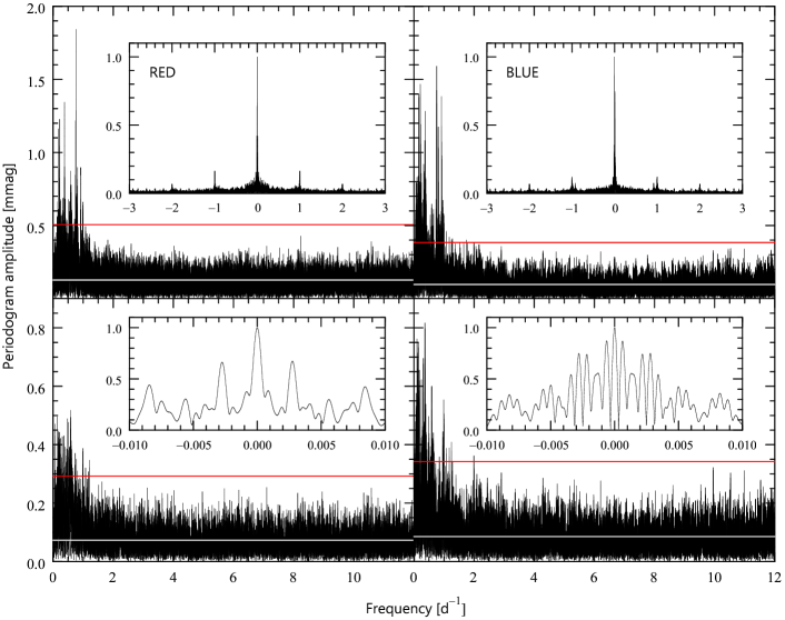
Figure 1: The amplitude spectra of the red and blue BRITE magnitudes pre-whitened with 2$f_{\rm orb}$ and of the residuals from the nine-frequency nonlinear least-squares fits (the upper and lower panels, respectively). The mean noise levels, computed from the amplitudes in the frequency range from 3.5 to 12 d^-1, are plotted with the white thick lines, and four times those, with the red lines. The spectral windows in the frequency range from $-$3 to 3 d^-1 are shown in the upper insets, and their central lobes, in the lower insets.

As can be seen from Table 2, the frequencies $f_{i}$ ($i={}$2,..,7,9) are related to each other and to $2f_{\rm orb}$:

$$f_{2}-f_{4}-2f_{\rm orb}=-0.000030\pm 0.000026\ {\rm d}^{-1},$$

$$f_{7}-f_{3}-2f_{\rm orb}=-0.000045\pm 0.000043\ {\rm d}^{-1},$$

$$f_{3}-f_{4}-f_{5}={}0.000010\pm 0.000051\ {\rm d}^{-1},$$

$$f_{6}-3f_{\rm orb}=-0.000006\pm 0.000010\ {\rm d}^{-1},$$

$$f_{9}-f_{\rm orb}=0.00006\pm 0.00012\ {\rm d}^{-1},$$

where the standard deviations were computed from the underestimated formal standard deviations of Table 2. Thus, with an accuracy better than 1$\sigma$ these interconnections lead to the following relations:

$$f_{2}-f_{4}=2f_{\rm orb},$$ (2)

$$f_{7}-f_{3}=2f_{\rm orb},$$ (3)

$$f_{5}=f_{3}-f_{4},$$ (4)

$$f_{6}=3f_{\rm orb},$$ (5)

$$f_{9}=f_{\rm orb},$$ (6)

illustrated in Fig. 2. Note that equation (4) can be replaced by

$$f_{5}=f_{7}-f_{2},$$ (7)

while equations (2) and (3) lead to

$$f_{2}+f_{3}=f_{4}+f_{7}.$$ (8)

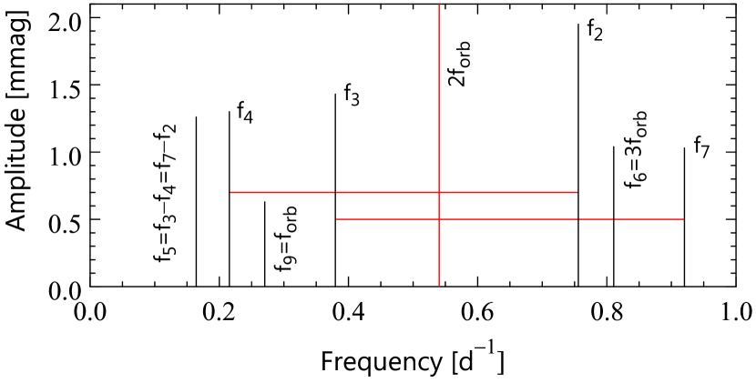
Figure 2: Schematic frequency spectrum of $\pi^{5}$ Ori plotted using the frequencies and the red amplitudes from Table 2. The $2f_{\rm orb}$ amplitude is off scale. The horizontal red lines represent the $2f_{\rm orb}$ separation between the doublets $f_{4},f_{2}$ and $f_{3},f_{7}$.

4 The orbital light and RV curves

The red- and blue-magnitude phase-diagrams are plotted in Fig. 3. The phases were computed with Miczaika’s (1950) orbital period of 3.700373 d and the epoch of phase zero HJD 2456900. The data shown as dots are normal points, formed in adjacent intervals of 0.01 orbital phase from the red and blue magnitudes pre-whitened with the $f_{i}$ ($i={}$2,..,5,7,8) terms using the parameters of the red and blue nonlinear least-squares fits of Section 3. Error bars are not plotted because they would rarely extend beyond the dots: the standard errors ranged from 0.10 to 0.28 mmag for the red normal points, and from 0.23 to 0.31 mmag for the blue normal points. The lines are the theoretical light-curves, computed from a Wilson-Devinney (W-D) solution obtained under assumption of synchronous rotation using the observed $V_{\rm rot}\sin i={}$90 km s^-1 (Głȩbocki & Gnaciński, 2005) and assuming the parameters $R_{1}={}$11.6 R_☉, $M_{1}={}$12.0 M_☉, $T_{\rm eff,1}={}$21 590 K for the primary component, and $R_{2}={}$2.83 R_☉, $M_{2}={}$4.95 M_☉, $T_{\rm eff,2}={}$16 500 K, and the radiative-envelope bolometric albedo $\alpha_{2}={}$1.0 for the secondary component, i.e. the first solution in Table 5. The W-D phase of the deeper minima is 0.6325. The depth difference between minima is equal to 3.5 and 2.0 mmag for the red and blue light-curves, respectively. In the W-D solutions, the reflection effect accounts for 2.1 mmag of the red depth difference and the entire blue depth difference. The W-D modeling will be discussed in Section B. Figure 4 is a frequency-domain counterpart of Fig. 3. In Fig. 4, the lines in the large panels are the amplitude spectra computed from the theoretical light-curves of ten cycles, while those in the insets, from the theoretical light-curves pre-whitened with the 2$f_{\rm orb}$ term. The circles are the amplitudes of the five-term Fourier-series least-squares fits to the normal points. The $f_{4}$ and $f_{6}$ terms were included in the fit so that their amplitudes could be compared with the theoretical ones. In both bands, the observed and theoretical amplitudes agree very well with each other.

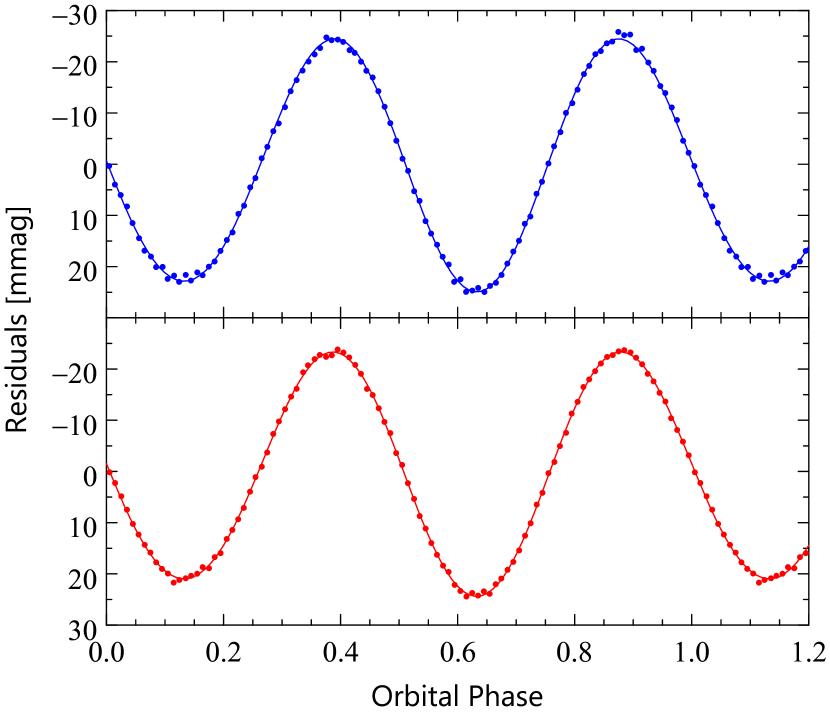
Figure 3: Normal points (dots), computed from the red (lower panel) and blue (upper panel) magnitudes pre-whitened with the $f_{i}$ ($i={}$2,..,5,7,8) terms using the parameters of the red and blue nonlinear least-squares fits of Section 3. The epoch of phase zero is HJD 2456900. The lines are the theoretical light-curves computed from the W-D solutions detailed in the text. The theoretical light-curves fit the normal points with standard deviations of 0.40 and 0.56 mmag for the red and blue data, respectively.

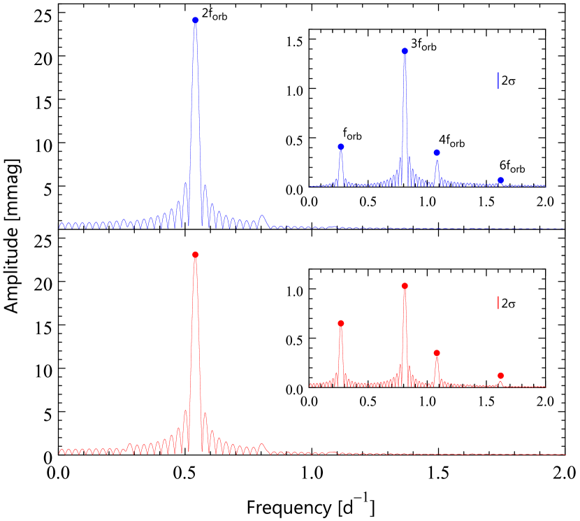
Figure 4: A frequency-domain counterpart of Fig. 3. The circles are the amplitudes of the five-term Fourier-series least-squares fits to the normal points. The error bars are labeled 2$\sigma$, where $\sigma$ is the formal least-squares standard deviation of the amplitudes. The lines in the large panels are the amplitude spectra computed from the W-D theoretical light-curves of ten cycles, while those in the insets, from the theoretical light-curves pre-whitened with the 2$f_{\rm orb}$ term.

Archival RVs of $\pi^{5}$ Ori are plotted in Fig. 5 together with an $e={}$0 orbital RV curve and the RV curve from the W-D solution mentioned in the preceding paragraph. The amplitude of the $e={}$0 curve $K_{1}={}$58.4$\pm$1.3 km/s and the phase of the minimum is equal to 0.879$\pm$0.004. The difference between the latter number and the above-mentioned phase of the deeper minima of the light-curves differs from the expected 0.25 by less than 1$\sigma$.

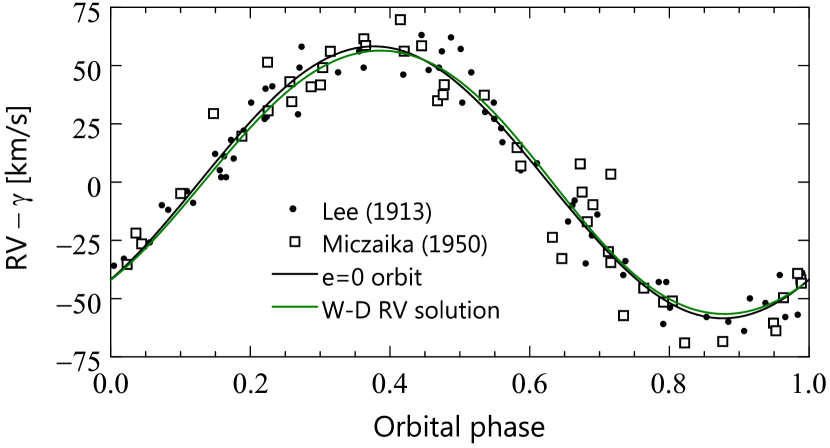
Figure 5: The archival RVs of $\pi^{5}$ Ori plotted as a function of phase of the orbital period. The epoch of phase zero is HJD 2456900. An $e={}$0 orbital RV curve and the RV curve from the W-D solution mentioned in the text are shown as the black and green line, respectively.

5 Discussion and conclusions

The system $\pi^{5}$ Ori is a simple one: the orbit is circular and the components can be safely assumed to rotate synchronously (see Levato, 1976, and references therein). Under such circumstances the tidal force does not change, resulting in the so-called equilibrium tide in which tidal distortion remains constant and the light-variation is caused by the variation of the projected area of the components as a function of phase of $2f_{\rm orb}$. The difference in the depth of the alternate minima seen in Fig. 3 reveals that in the case of $\pi^{5}$ Ori this ellipsoidal variation is modified by a small but significant reflection effect. Under the assumption of synchronous rotation, the best fits of the W-D to the observed light-curves are obtained for $M_{1}={}$12 M_☉ with $\log T_{\rm eff,1}$ and $\log L_{1}/$L_☉ within 1$\sigma$ of the HR diagram position of the star derived in Section A from photometric data from the literature and the Hipparcos parallax and in limited ranges of $\log T_{\rm eff,2}$, different for the two cases we consider, viz. that of a radiative-envelope bolometric albedo $\alpha_{2}={}$1.0 and a convective-envelope bolometric albedo $\alpha_{2}={}$0.5 (see Table 3). The primary component of $\pi^{5}$ Ori is thus found to be in a more advanced stage of evolution than components of the SB2 eclipsing binaries of comparable masses in table 1 of Torres, Andersen & Gimenénez (2010). Although the magnitude difference between the components is not known, we derive duplicity corrections for the two cases of the bolometric albedo of the secondary using magnitude differences from the W-D modeling and assuming that $M_{2}$, the secondary component’s mass from the orbital solution is equal to its evolutionary mass (see Tables 4 and 5 and Fig. 7). A comparison of the evolutionary age of the secondary with that of the primary shows that in the $\alpha_{2}={}$0.5 case the evolutionary age is over an order of magnitude too small, while in the $\alpha_{2}={}$1.0 case the difference of the evolutionary masses is probably within the uncertainties of the analysis, suggesting that the secondary is in an early stage of its MS evolution (open triangle at lower right in Figs. 7 and 8).

In addition to causing the ellipsoidal light-variation, the equilibrium tide modifies the frequencies of the self-driven pulsations of the components. According to the theoretical work of Reyniers & Smeyers (2003) and Smeyers (2005), summarized recently by Balona (2018), a non-radial pulsation mode perturbed by an equilibrium tide can be described by a set of independent modes that are associated with a single spherical harmonic $Y_{\ell}^{m}(\theta,\phi)$ where $\theta$ and $\phi$ are the polar and azimuthal angles in a spherical coordinate system whose polar axis coincides with the line joining the components’ mass centres. In the corotating frame, each $2(\ell+1)$-fold degenerate eigenfrequency of a mode $n$ is split into $\ell+1$ eigenfrequencies. In the non-rotating frame with the polar axis parallel to the pulsating component’s rotation axis, an $\ell=1$, $m=0$ eigenfrequency is split into two frequencies, while that of the $\ell=1$, $m=1$ eigenfrequency, into three frequencies. To first-order in a small dimensionless parameter $\epsilon_{T}=(R/a)^{3}q$, where $R$ is the radius of the pulsating component and $q$ is the mass ratio, the two $\ell=1$, $m=0$ frequencies, $f^{(1,0)}_{1}$ and $f^{(1,0)}_{2}$ are given by:

$$f^{(1,0)}_{1}=f_{n,0}+\epsilon_{T}f^{(1,0)}_{n,1}-\Omega/2\pi,$$ (9)

$$f^{(1,0)}_{2}=f_{n,0}+\epsilon_{T}f^{(1,0)}_{n,1}+\Omega/2\pi,$$ (10)

while the three $\ell=1$, $m=1$ frequencies, $f^{(1,1)}_{1}$, $f^{(1,1)}_{2}$ and $f^{(1,1)}_{3}$, by:

$$f^{(1,1)}_{1}=f_{n,0}+\epsilon_{T}f^{(1,1)}_{n,1}-\Omega/2\pi,$$ (11)

$$f^{(1,1)}_{2}=f_{n,0}+\epsilon_{T}f^{(1,1)}_{n,1},$$ (12)

$$f^{(1,1)}_{3}=f_{n,0}+\epsilon_{T}f^{(1,1)}_{n,1}+\Omega/2\pi,$$ (13)

where $f_{n,0}$ is the eigenfrequency of the unperturbed mode, $\epsilon_{T}f^{(\ell,m)}_{n,1}$ are the first order corrections to $f_{n,0}$, and $\Omega$ is the angular velocity of rotation. In the case of $\ell=2$, $|m|\leq\ell$, the $\ell+1$ eigenfrequencies would be split into 12 frequencies that include an equidistant triplet, quadruplet and quintuplet; in the case of $\ell=3$, the eigenfrequencies split into 24 frequencies that include an equidistant quadruplet, sextuplet and two septuplets (see table 1 and fig. 2 of Balona, 2018). In the frequency spectrum of a pulsating component, the frequencies $f^{(1,0)}_{1}$ and $f^{(1,0)}_{2}$ would form a doublet with separation equal to $\Omega/\pi=2f_{\rm orb}$, while frequencies $f^{(1,1)}_{1}$, $f^{(1,1)}_{2}$ and $f^{(1,1)}_{3}$, an equidistant triplet with the separation equal to $\Omega/2\pi=f_{\rm orb}$. As can be seen from Fig. 2, in the frequency spectrum of $\pi^{5}$ Ori there are two doublets separated by $2f_{\rm orb}$, viz. $f_{4},f_{2}$ and $f_{3},f_{7}$, but no equidistant triplets. From equations (9)-(13) we conclude that two $l=1,m=0$ modes, $n$ and $n^{\prime}$, are excited in the primary component of $\pi^{5}$ Ori. Using $R_{1}$, $M_{1}$ and $M_{2}$ from Table 5, we get $\epsilon_{T}<0.05$. Neglecting the second term on the rhs of equations (9) and (10), we obtain approximate values of the unperturbed frequencies, $f_{n,0}\approx f_{2}-f_{\rm orb}=f_{4}+f_{\rm orb}=(f_{2}+f_{4})/2=0.49$ d^-1 and $f_{n^{\prime},0}\approx f_{3}+f_{\rm orb}=f_{7}-f_{\rm orb}=(f_{3}+f_{7})/2=0.65$ d^-1. These values of $f_{n,0}$ and $f_{n^{\prime},0}$ are characteristic of high-order $\ell=1$ gravity modes, so that $\pi^{5}$ Ori should be classified as an ellipsoidal SPB variable or ELL/LPB(LBV) in the parlance of the General Catalogue of Variable Stars.

The first order combination terms between the modes $n$ and $n^{\prime}$ have the following frequencies

$$f_{n,0}+f_{n^{\prime},0}=f_{2}+f_{3}-\epsilon_{T}\left(f^{(1,0)}_{n,1}+f^{(1,0)}_{n^{\prime},1}\right)$$

$$=f_{4}+f_{7}-\epsilon_{T}\left(f^{(1,0)}_{n,1}+f^{(1,0)}_{n^{\prime},1}\right)$$ (14)

and

$$f_{n^{\prime},0}-f_{n,0}=f_{3}-f_{4}+\epsilon_{T}\left(f^{(1,0)}_{n,1}-f^{(1,0)}_{n^{\prime},1}\right)$$

$$=f_{7}-f_{2}+\epsilon_{T}\left(f^{(1,0)}_{n,1}-f^{(1,0)}_{n^{\prime},1}\right).$$ (15)

Given negligible first-order corrections $\epsilon_{T}f^{(1,0)}$, equations (15) are consistent with equations (4) and (7), while equations (14), with equations (8).

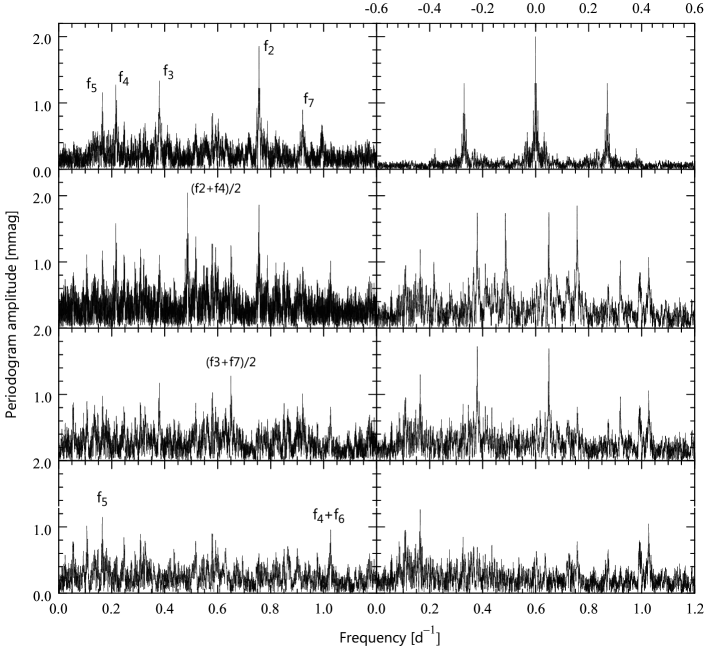
Figure 6: The amplitude spectra of three sets of the BRITE red magnitudes of $\pi^{5}$ Ori pre-whitened with the orbital light-variation: (1) all magnitudes (the top left-hand panel), (2) the magnitudes covering orbital phases from the western to eastern quadrature, i.e. the phases from 0.3825 to 0.8825 in Figs. 3 and 5 (the remaining left-hand panels), and (3) the magnitudes covering the remaining orbital phases, i.e. the phases from 0 to 0.3825 and from 0.8825 to 1 in Figs. 3 and 5 (the right-hand panels, from upper middle to bottom). The top right-hand panel shows the spectral window of set 3; at the resolution of the figure, the spectral window of set 2 would be very nearly identical with the one shown. The lower middle and bottom panels show the amplitude spectra of the set 2 and 3 data pre-whitened with $f_{n,0}=(f_{2}+f_{4})/2={}$0.4857 d^-1, and with this frequency and $f_{n^{\prime},0}=(f_{3}+f_{7})/2={}$0.6500 d^-1, respectively.

The referee has suggested a test that our $f_{n,0}$ and $f_{n^{\prime},0}$ modes are indeed associated with the $\ell=1$, $m=0$ spherical harmonics and provided examples of applying the test to simulated data. The test consists in dividing the data into two parts according to the orbital phase in such a way that one part contains the data covering orbital phases from one quadrature to the other, and the second part, the remaining data, and then computing amplitude spectra for the two parts separately. Using simulated $\ell=1$, $m=0$ light-curves with an assumed pulsation frequency, Reed, Brondell & Kawaler (2005) found for a range of inclination of the pulsation axis to the line of sight that in the amplitude spectra of the two parts of the data there appears a peak at the assumed frequency flanked by $f_{\rm orb}$ aliases whereas in the amplitude spectrum of the complete data set the peak at the assumed frequency is missing (see their figure 4). In addition, there is a phase difference equal to $\pi$ between the light-curves in the two parts of the data. For the test, we used the red BRITE magnitudes because their spectral window is cleaner than that of the blue magnitudes (see the insets in the lower panels of Fig. 1). We removed the orbital light-variation by pre-whitening with $f_{\rm orb}$, 2$f_{\rm orb}$, 3$f_{\rm orb}$, 4$f_{\rm orb}$ and 6$f_{\rm orb}$, divided the data into two parts as described above, and computed amplitude spectra. The results are displayed in Fig. 6. The top left-hand panel shows the amplitude spectrum of the complete data (referred to as set 1 in the caption to the figure) with the peaks at the frequencies appearing in equations (2)-(5) labelled. The upper middle left-hand panel shows the amplitude spectrum of the magnitudes covering the orbital phases from the western to eastern quadrature, i.e. the phases from 0.3825 to 0.8825 in Figs. 3 and 5 (set 2). The peak at $f_{n,0}=(f_{2}+f_{4})/2={}$0.4857 d^-1 and its $f_{\rm orb}$ aliases dominate the spectrum. The aliases occur at the same frequencies as the $f_{2}$ and $f_{4}$ peaks in the top left-hand panel but should not be confused with them. While the aliases reproduce the side-lobes of the spectral window seen in the top right-hand panel, the frequencies $f_{2}$ and $f_{4}$ arise as the result of a transformation of the corotating frame of reference whose polar axis coincides with the line joining the components’ mass centres to the non-rotating frame with the polar axis parallel to the pulsating component’s rotation axis (see the second paragraph of this section). The lower middle left-hand panel contains the amplitude spectrum obtained from the set 2 data pre-whitened with $f_{n,0}$. Now, the highest peak appears at $f_{n^{\prime},0}=(f_{3}+f_{7})/2={}$0.6500 d^-1. Finally, the amplitude spectrum of the set 2 data pre-whitened with $f_{n,0}$ and $f_{n^{\prime},0}$ is shown in the bottom left-hand panel. Here, the two highest peaks appear at 0.1643 d${}^{-1}{}=f_{5}$ and 1.0262 d${}^{-1}{}=f_{4}+f_{6}$. The amplitude spectra of the second part of the data, i.e. the data covering orbital phases from 0 to 0.3825 and from 0.8825 to 1 in Figs. 3 and 5 (set 3) are shown in three right-hand panels. The amplitude spectra in the right-hand middle panels differ in appearance from their left-hand counterparts but still the peaks at the frequencies $f_{n,0}$, $f_{n^{\prime},0}$ and their $f_{\rm orb}$ aliases are the strongest features present. The phases of the $f_{n,0}$ and $f_{n^{\prime},0}$ light-curves computed for set 2 and 3 separately are equal to 5.500$\pm$0.022 and 2.689$\pm$0.025 rad for $f_{n,0}$ and 2.524$\pm$0.029 and 5.351$\pm$0.026 rad for $f_{n^{\prime},0}$. The phase differences between the light-curves of set 2 and 3 amount to (0.895$\pm$0.011)$\pi$ and ($-$0.900$\pm$0.012)$\pi$ for $f_{n,0}$ and $f_{n^{\prime},0}$, respectively. The outcome of the test is thus mixed: the amplitudes of the $f_{n,0}$ and $f_{n^{\prime},0}$ modes behave as predicted by the $\ell=1$, $m=0$ simulations of Reed et al. (2005) but the phase differences, although close to, are significantly smaller than $\pi$, even if the formal standard deviations were to be underestimated by a factor of two as maintained in Section 3.

The highest peak in the bottom left-hand panel of Fig. 6 at the combination frequency $f_{5}=f_{n^{\prime},0}-f_{n,0}$, mentioned earlier in this section, has very nearly the same amplitude in the bottom right-hand and top left-hand panels. One would therefore expect that the $f_{5}$ light-curves of set 2 and 3 will be in phase. In fact, the phases are equal to 4.860$\pm$0.037 and 4.559$\pm$0.035 rad, so that the light-curves differ in phase by (0.096$\pm$0.016)$\pi$. If we were to take this result as an indication that the standard deviations of the phase differences are underestimated by a factor of about six instead of two, the deviations of the phase differences from $\pi$ noted at the end of the preceding section would become tolerable. The second highest peak in the bottom panels of Fig. 6 occurs at the frequency $f_{4}+f_{6}$. It has no counterpart in the top left-hand panel or in the left-hand panels of Fig. 1. Now the phase difference between sets 2 and 3 amounts to (0.962$\pm$0.020)$\pi$, as one would expect.

In closing, we would like to venture a prediction: frequencies resulting from the tidal splitting of the the $\ell=1$, $m=1$ and $\ell=2$, $|m|\leq\ell$ eigenfrequencies will be eventually identified at the low end of the frequency axis where the present analysis failed (see Fig. 1).

Appendix A Fundamental Parameters

Let us start with deriving the colour excess of $\pi^{5}$ Ori. From the Strömgren indices $b-y$ and $c_{1}$ (Hauck & Mermilliod, 1998) we get $c_{0}={}$0.125, $(b-y)_{0}={}-$0.105, $E(b-y)={}$0.044 and $E(B-V)={}$0.059 mag by means of the canonical method of Crawford (1978). From the $UBV$ colour indices (Mermilliod, 1991) and the standard two-colour relation for luminosity class III B-type stars (Johnson, 1963) we get $E(B-V)={}$0.058 mag. The excellent agreement of these values of $E(B-V)$ may be somewhat accidental.

We shall now use $c_{0}$ to estimate the effective temperature, $T_{\rm eff,1}$, and the bolometric correction, $BC_{1}$, of the primary component of $\pi^{5}$ Ori assuming negligible brightness of the secondary. We get $T_{\rm eff,1}={}$21 125 K and $BC_{1}={}-$2.14 mag using the calibration of Davis & Shobbrook (1977), $T_{\rm eff,1}={}$21 314 K using UVBYBETA and 21 154 K using the calibration of Sterken & Jerzykiewicz (1993). The close agreement between these $T_{\rm eff}$ values is due to the fact that the three temperature calibrations rely heavily on the OAO-2 absolute flux calibration of Code et al. (1976). Taking a straight mean of the above three values we arrive at $T_{\rm eff,1}=21\,200$ K. Realistic standard deviations of the effective temperatures of early-type stars, estimated from the uncertainty of the absolute flux calibration, amount to about 3 % (Napiwotzki et al., 1993; Jerzykiewicz, 1994) or 640 K for the $T_{\rm eff,1}$ in question, so that $\log T_{\rm eff,1}={}$4.326$\pm$0.013. The standard deviation of $BC_{1}$ we estimate to be 0.20 mag.

The revised Hipparcos parallax of $\pi^{5}$ Ori is equal to 2.43$\,\pm\,$0.39 mas (van Leeuwen, 2007). Taking the star’s $V$ magnitude from Mermilliod (1991), $E(B-V)$ from the first paragraph of this section, and assuming $R_{V}={}$3.2, we get $M_{V}={}-$4.54${}^{+\rm 0.32}_{-\rm 0.38}$ mag, $M_{\rm bol}={}-$6.68${}^{+\rm 0.38}_{-\rm 0.43}$ mag, and $\log L_{1}/{\rm L}_{\sun}={}$4.57${}^{+\rm 0.17}_{-\rm 0.15}$. In computing $\log L_{1}/$L_☉, we assumed M${}_{{\rm bol}{\sun}}={}$4.74 mag, a value consistent with BC${}_{\sun}=-{}$0.07 mag and $V_{\sun}={}-$26.76 mag (Torres, 2010).

In Fig. 7, $\pi^{5}$ Ori is plotted in the HR diagram together with the 4, 5, 10, 12 and 15 M_☉ Padova evolutionary tracks from Bertelli et al. (2009) for $Y={}$0.26 and $Z=0.017$, and the 4 and 5 M_☉ Pisa pre-MS tracks from Tognelli, Prada Moroni & Degl’Innocenti (2011) for $Y={}$0.265, $Z={}$0.0175 and the mixing-length parameter of 1.68 $H_{\rm p}$, where $H_{\rm p}$ is the pressure scale height. As can be seen from the figure (see the inset), the star falls to the right and above the terminal main-sequence (TAMS) but is off the region corresponding to the late hydrogen-burning (HB) evolutionary stage by less than 1$\sigma$ in $\log T_{\rm eff}$ and in $\log L/{\rm L}_{\sun}$. The green inverted triangles, black circles and red squares (open and filled, connected with straight lines and otherwise) are from the W-D solutions discussed in Section B.

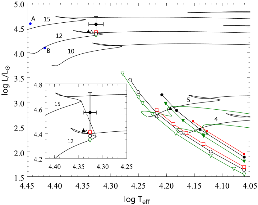
Figure 7: The components of $\pi^{5}$ Ori in the HR diagram. The diamond with error bars is plotted using $\log(T_{\rm eff,1}={}$21 200 K$)$ and $\log L_{1}/{\rm L}_{\sun}$ derived in Section A under assumption of negligible brightness of the secondary component. The green open inverted-triangles, black open circles and red open squares are from the W-D solutions for $M_{1}={}$11, 12 and 13 M_☉, respectively, $T_{\rm eff,1}={}$21 200 K, a radiative-envelope bolometric albedo $\alpha_{1}=\alpha_{2}={}$1.0 and a range of $\log T_{\rm eff,2}$, while the green filled inverted-triangles, black filled circles and red filled squares are from the W-D solutions with the same $M_{1}$, $T_{\rm eff,1}$ and $\alpha_{1}$ as above, a convective-envelope bolometric albedo $\alpha_{2}={}$0.5 and a range of $\log T_{\rm eff,2}$. The $\log T_{\rm eff,2}$ ranges are specified in Section B where the W-D solutions are discussed. The primary component’s HR diagram positions from the W-D solutions (open inverted-triangle, open circle and open square at upper left and in the inset) were virtually unaffected by the assumed values of the secondary’s albedo and effective temperature. The W-D duplicity-corrected positions of both components (black open and filled triangles for $\alpha_{2}={}$1.0 and 0.5, respectively) are plotted using the parameters from Table 5; the filled triangle representing the primary component (upper left and the inset) was shifted by 0.004 dex to the left to avoid overlap. The blue dots represent components of the detached eclipsing binary V453 Cyg plotted using the data from table 1 of Torres et al. (2010) to be referred to in the last paragraph of Section B. Also plotted are the 4, 5, 10, 12 and 15 M_☉ Padova evolutionary tracks for $Y={}$0.26 and $Z={}0.017$ (black lines) from Bertelli et al. (2009), and the 4 and 5 M_☉ Pisa pre-MS tracks from Tognelli et al. (2011) for $Y={}$0.265, $Z={}$0.0175 and the mixing-length parameter of 1.68 $H_{\rm p}$, where $H_{\rm p}$ is the pressure scale height (dark-green lines). In the inset, the TAMS is indicated (short-dashed line).

The surface gravity of a B-type star can be obtained from its $\beta$ index. There are two values of the $\beta$ index of $\pi^{5}$ Ori in the literature: 2.603 (Hauck & Mermilliod, 1998) and 2.597 mag (Paunzen, 2015). From a straight mean of these numbers and $T_{\rm eff}$, we get $\log g={}$3.40 using the $T_{\rm eff}$, $\beta$ grid of Smalley & Dworetsky (1995) modified by Dziembowski & Jerzykiewicz (1999). According to Napiwotzki et al. (1993), the uncertainty of the $\beta$-index surface gravities of hot stars is equal to 0.25 dex; we shall adopt this value as the standard deviation of the star’s $\log g$. Using the above derived $T_{\rm eff}={}$21 200$\,\pm\,$640 K and $\log g={}$3.40$\,\pm\,$0.25, we plot $\pi^{5}$ Ori in Fig. 8 together with the MS and pre-MS evolutionary tracks, and $\log g$ resulting from the W-D modeling to be discussed in Section B.

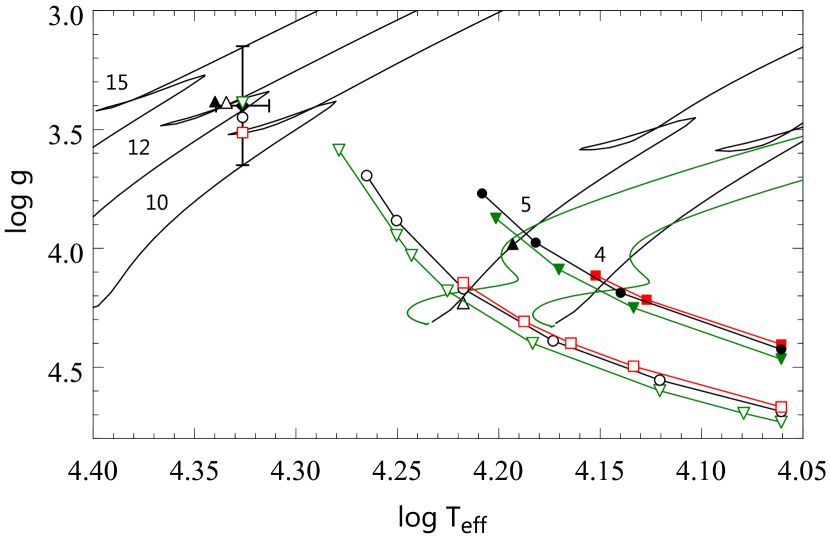
Figure 8: The components of $\pi^{5}$ Ori in the $\log T_{\rm eff}$, $\log g$ plane. The symbols are the same as in Fig. 7 except that the black open circle and red open square at upper left, representing the position of the primary from the 12 and 13 M_☉ W-D solutions, were shifted downwards by 0.06 and 0.12 dex, respectively, to avoid overlap. Also plotted are the evolutionary tracks from the sources referenced in the caption to Fig. 7.

The 2016 version of the PASTEL catalogue (Soubiran et al., 2016) lists $T_{\rm eff}={}$21 860 K and $\log g={}$3.51 obtained by Gies & Lambert (1992) from Strömgren colour indices and H$\gamma$ line profiles through a comparison with colours and line profiles from Kurucz line-blanketed atmospheres. These values agree quite well with those we derived: the former is greater than ours by slightly more than 1$\sigma$, while the latter, by less than 0.5$\sigma$.

Appendix B The W-D Modeling

The light-curves shown in Fig. 3 as dots were subject to modeling by means of the 2015 version of the Wilson-Devinney code (hereafter W-D, Wilson & Devinney, 1971; Wilson, 1979). In the modeling, we used Miczaika’s (1950) orbital period of 3.700373 d and the semi-amplitude of the RV curve $K_{1}={}$58.4 km s^-1 obtained in Section 4 from the combined observations of Lee (1913) and Miczaika (1950) assuming zero eccentricity. For both components, the limb darkening coefficients were taken from the logarithmic-law tables of Walter V. Van Hamme. We assumed [M/H] $=0$ and used $\lambda$421 and 620.5 nm monochromatic coefficients for the blue and red data, respectively. In treating the reflection effect, we used the detailed model with six reflections (MREF $=2$, NREF $=6$). The reflection effect is small but significant: it accounts for the difference in the depth of the minima seen in Fig. 3. Under assumption of synchronous rotation, the observed $V_{\rm rot}\sin i={}$90 km s^-1 (Głȩbocki & Gnaciński, 2005) and the radius of the primary component yield the inclination of the orbit. For a given $M_{1}$, one then gets $M_{2}$. Guided by the position of the star in the HR diagram in relation to the evolutionary tracks (see Fig. 7), we assumed $M_{1}\leq{}$15 M_☉ and then computed W-D solutions for $M_{1}={}$10, 11, 12, 13, 14 and 15 M_☉, a $\pm$640 K range of $T_{\rm eff,1}$ around $T_{\rm eff,1}={}$21 200 K, the value derived in Section A, a number of values of $T_{\rm eff,2}$, and the primary’s radiative-envelope bolometric albedo $\alpha_{1}={}$1.0. Since the evolutionary state of the secondary is not known, we computed two series of solutions, one with the secondary’s bolometric albedo $\alpha_{2}={}$1.0, and the other, with a convective-envelope bolometric albedo $\alpha_{2}={}$0.5. We found that the overall standard deviation, $SD_{\rm ov}$, of the W-D fit to the observed light-curves is a function of $M_{1}$ and $T_{\rm eff,2}$. This result is set out in Fig. 9 with $\log T_{\rm eff,2}$ as the abscissa. As can be seen from the figure, the best fits are obtained for $M_{1}={}$12 M_☉, $\alpha_{2}={}$1.0, $\log T_{\rm eff,2}\leq{}$4.22, and $\alpha_{2}={}$0.5, $\log T_{\rm eff,2}\approx{}$4.06. For $M_{1}={}$10, 14 and 15 M_☉, the fits are much less satisfactory. The parameters’ ranges from the solutions which yield fits with $SD_{\rm ov}\leq 0.495$ mmag are listed in Table B1. The parameters of these solutions were used to plot the components in Figs. 7 and 8. As can be seen from Table 3, the primary’s W-D radius and luminosity are not sensitive to the secondary’s effective temperature and albedo, so that for given $M_{1}$ and $T_{\rm eff,1}$, $R_{1}$, $M_{2}$ and the primary’s HR diagram position remain nearly unchanged. In contrast, $R_{2}$ and the HR diagram position of the secondary vary strongly with $T_{\rm eff,2}$. We shall take advantage of the last property in the next paragraph.

Table 3: The parameters of the W-D solutions which yield fits to the observed light-curves of Fig. 3 with the overall standard deviation $SD_{\rm ov}\leq 0.495$ mmag.

$M_{1}$	$\alpha_{2}$	$R_{1}$	$i$	$\log L_{1}/$L☉	$\log g_{1}$	$\log T_{\rm eff,2}$	$R_{2}$	$\log L_{2}/$L☉	$\log g_{2}$
[M☉]		[R☉]					[R☉]
11	1.0	11.0-11.4	36$\aas@@fstack{\circ}$6-35$\aas@@fstack{\circ}$3	4.34-4.37	3.39-3.36	4.061-4.279	1.50-5.70	1.54-3.58	4.73-3.59
11	0.5	11.1-11.3	36$\aas@@fstack{\circ}$5-35$\aas@@fstack{\circ}$8	4.34-4.36	3.39-3.38	4.061-4.201	2.04-4.06	1.81-2.97	4.47-3.87
12	1.0	11.5-11.8	34$\aas@@fstack{\circ}$7-33$\aas@@fstack{\circ}$8	4.38-4.40	3.39-3.37	4.061-4.265	1.66-5.30	1.63-3.45	4.69-3.69
12	0.5	11.5-11.7	34$\aas@@fstack{\circ}$8-34$\aas@@fstack{\circ}$2	4.38-4.39	3.39-3.38	4.061-4.208	2.24-4.82	1.89-3.15	4.42-3.77
13	1.0	12.0-12.1	33$\aas@@fstack{\circ}$3-33$\aas@@fstack{\circ}$0	4.41-4.42	3.40-3.39	4.061-4.218	1.78-3.26	1.69-2.84	4.67-4.14
13	0.5	12.0-12.1	33$\aas@@fstack{\circ}$3-33$\aas@@fstack{\circ}$1	4.41-4.42	3.39-3.39	4.061-4.152	2.41-3.38	1.96-2.61	4.40-4.11

Since the magnitude difference between the components of $\pi^{5}$ Ori is not known, we cannot correct the parameters of the primary component derived in Section A from the combined-light magnitude and colour indices for the light dilution caused by the secondary. However, using magnitude differences provided by the W-D solutions we can compute duplicity corrections for a given $T_{\rm eff,1}$ (uncorrected), $M_{1}$ and $T_{\rm eff,2}$. As an example, we chose the $T_{\rm eff,1}={}$21 200 K, $M_{1}={}$12 M_☉, $\alpha_{2}={}$1.0 and 0.5 solutions with $T_{\rm eff,2}$ selected in such a way that the evolutionary masses estimated from the evolutionary tracks shown in Fig. 7 were equal to $M_{2}$, viz. $T_{\rm eff,2}={}$16 400 K for $\alpha_{2}={}$1.0 and the MS Padova tracks, and $T_{\rm eff,2}={}$15 400 K for $\alpha_{2}={}$0.5 and the pre-MS Pisa tracks. Taking the blue ($\lambda$421 nm) and red ($\lambda$620.5 nm) magnitude differences from these solutions we obtained the $V$ ($\lambda$555 nm) magnitude difference $\Delta V={}$3.2 and 2.8 mag for $\alpha_{2}={}$1.0 and 0.5, respectively. Assuming luminosity class V for the secondary, we estimated its spectral type from the tables of Lang (1992) to be B6.7 and B5.3 for $\Delta V={}$3.2 and 2.8 mag, respectively. Then, from the average values of $c_{0}$ and $m_{0}$ as a function of MK type and the average values of $(b-y)_{0}$ as a function of $c_{0}$ (tables II and I of Crawford, 1978) we obtained the duplicity corrections (to be subtracted from the combined $c_{0}$) of 0.015 and 0.018 mag for $\Delta V={}$3.2 and 2.8 mag, respectively. In terms of $T_{\rm eff}$, the correction (to be added to the observed value) is 390 and 470 K, respectively. The duplicity correction to $\beta$ was computed assuming that for single stars $\beta_{\rm wide}$ scales as the magnitude at 486 nm. Assuming again luminosity class V for the secondary, we then get the duplicity correction (to be subtracted from the combined $\beta$) of 0.005 and 0.007 mag for $\Delta V={}$3.2 and 2.8 mag. Consequently, the corrections to be subtracted from $\log g$ obtained from the combined $\beta$ and $c_{0}$ are equal to 0.07 and 0.03 dex for $\Delta V={}$3.2 and 2.8 mag, respectively. The corrections for the different $\Delta V$ differ because the duplicity-corrected $c_{0}$ differ. Finally, the corrections to $\log L/$L_☉ (to be subtracted from the uncorrected values), with the corrections to $BC$ taken into account, were equal to 0.006 and 0.014 dex for $\Delta V={}$3.2 and 2.8 mag, respectively. The duplicity-corrected photometric indices and fundamental parameters of the primary component are listed in Table 4, and its duplicity-corrected positions are shown in Figs. 7 and 8 as the triangles at upper left. With the duplicity-corrected $T_{\rm eff,1}$, we obtained solutions for $M_{1}={}$12 M_☉ for which $M_{2}$ were equal to the evolutionary masses. The parameters of these solutions are listed in Table 5. Note that the primary’s W-D luminosities are lower than the duplicity-corrected value by slightly less than 1$\sigma$.

The problem with the above example is that the evolutionary ages do not match: the TAMS age on the 12 M_☉ track is equal to 18 Myr while the evolutionary ages on the 5 M_☉ tracks are equal to 25 Myr for the secondary component on the MS track ($\alpha_{2}={}$1.0), and 0.8 Myr for the secondary on the pre-MS track ($\alpha_{2}={}$0.5). The 18 Myr evolutionary age of the $\alpha_{2}={}$1.0 secondary would result if we shifted the 5 M_☉ MS track by $-$0.013 dex in $\log T_{\rm eff}$ and by $-$0.11 dex in $\log L/$L_☉. A similar result would be obtained by appropriately shifting the HR diagram position of the secondary. In view of the uncertainties of our data (e.g. those of the evolutionary tracks on the theoretical side, and $V_{\rm rot}\sin i$ on the observational side) the mismatch of the components’ evolutionary masses for the $\alpha_{2}={}$1.0 solution is tolerable. However, it is certainly not for the $\alpha_{2}={}$0.5 solution. Thus, our example suggests that the secondary component is in the early stages of its MS evolution (open triangle at lower right in Figs. 7 and 8). This conclusion is in keeping with the fact, seen in Fig. 9, that the $SD_{\rm ov}$ for the $\alpha_{2}={}$1.0 solutions are lower than those for the $\alpha_{2}={}$0.5 solutions.

Table 4: The duplicity-corrected photometric indices and fundamental parameters of the primary component of $\pi^{5}$ Ori for the two values of the magnitude difference between the components, $\Delta V$, obtained from the $M_{1}={}$12 M_☉, $T_{\rm eff,1}={}$21 200 K W-D solutions discussed in Section B.

$\alpha_{2}$	$\Delta V$	$c_{0}$	$\beta$	$T_{\rm eff,1}$	$\log L_{1}/$L☉	$\log g_{1}$
1.0	3.2	0.110	2.595	21 590$\pm$650	4.564$\pm$0.16	3.33$\pm$0.25
0.5	2.8	0.107	2.593	21 670$\pm$650	4.556$\pm$0.16	3.36$\pm$0.25

Table 5: The parameters of the components of $\pi^{5}$ Ori obtained from the W-D solutions for $M_{1}={}$12 M_☉ and the duplicity-corrected $T_{\rm eff,1}$ listed in Table 4.

$\alpha_{2}$	$R_{1}$	$i$	$a$	$M_{2}$	$\log T_{\rm eff,2}$	$R_{2}$	$\log L_{1}/$L☉	$\log L_{2}/$L☉	$\log g_{1}$	$\log g_{2}$	$SD_{\rm ov}$
	[R☉]		[R☉]	[M☉]		[R☉]					[mmag]
1.0	11.6	34$\aas@@fstack{\circ}$4	25.9	4.95	4.218	2.83	4.42	2.72	3.39	4.24	0.484
0.5	11.7	34$\aas@@fstack{\circ}$3	25.9	4.96	4.193	3.76	4.43	2.87	3.38	3.98	0.488

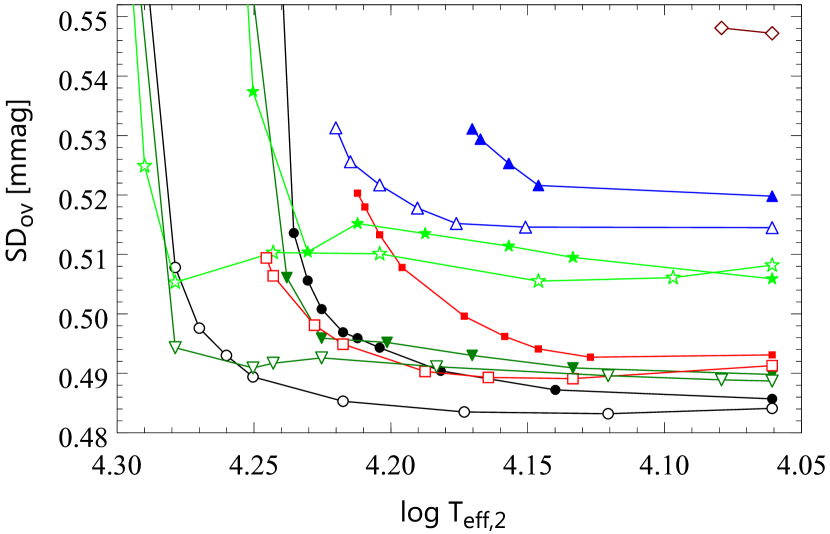
Figure 9: The overall standard deviation, $SD_{\rm ov}$, of the W-D fits to the observed light-curves of Fig. 3 for $T_{\rm eff,1}={}$21 200 K and $M_{1}={}$10 (light-green asterisks), 11 (dark-green inverted triangles), 12 (black circles), 13 (red squares), 14 (blue triangles) and 15 M_☉ (brown diamonds). Empty symbols represent solutions with $\alpha_{2}={}$1.0, filled symbols, with $\alpha_{2}={}$0.5. For $M_{1}={}$13, 14 and 15 M_☉, the primary component exceeded its critical lobe in the solutions on the left-hand side of the last plotted point; for $M_{1}={}$15 M_☉ and $\alpha_{2}={}$0.5, the primary component exceeded its critical lobe if $\log T_{\rm eff,2}\geq{}$4.03.

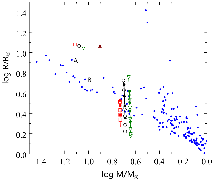
Figure 10: The radii of the components of $\pi^{5}$ Ori, obtained from the W-D solutions with $T_{\rm eff,1}={}$21 200 K, $M_{1}={}$11, 12 and 13 M_☉ (green inverted triangles, black circles and red squares, respectively), the same as those used in plotting Figs. 7 and 8, compared with the empirical masses and radii of the SB2 eclipsing binaries from table 1 of Torres et al. (2010) (blue dots; those labeled A and B represent components of the detached eclipsing binary V453 Cyg). The primary component’s radii (open inverted triangle, open circle and open square at upper left) were unaffected by the assumed value of the secondary’s bolometric albedo and effective temperature. The secondary’s radii from the $M_{1}={}$12 M_☉ and duplicity-corrected $T_{\rm eff,1}$ solutions, listed in the seventh column of Table 5, are shown as black open and filled triangles for $\alpha_{2}={}$1.0 and 0.5, respectively; the primary’s radii from these solutions are not plotted because they would coincide with the open circle at upper left. The brown triangle is from Morris’ (1985) solution with negligible brightness of the secondary component; $\log R_{1}/$R_☉ from his other solution differs from that shown by an insignificant 0.05.

The radii of the components of $\pi^{5}$ Ori derived from the $M_{1}={}$11, 12 and 13 M_☉ W-D solutions given in Table 3 are compared in Fig. 10 with the empirical masses and radii of the SB2 eclipsing binaries from table 1 of Torres et al. (2010). As can be seen from the figure, good agreement of the W-D radii of the secondary component with the empirical ones is obtained over the whole interval of $\log T_{\rm eff,2}$ listed in Table 3 for $\alpha_{2}={}$0.5 (filled inverted triangles, filled circles and filled squares), and over the $\log T_{\rm eff,2}$ intervals [4.17,4.27], [4.16,4.26] and [4.14,4.22] for $\alpha_{2}={}$1.0, $M_{1}={}$11, 12 and 13 M_☉, respectively (open inverted triangles, open circles and open squares). The secondary’s radii from the $M_{1}={}$12 M_☉ and duplicity-corrected $T_{\rm eff,1}$ solutions given in Table 5 (black open and filled triangles) fall within the [4.16,4.26] interval. However, the primary’s W-D radii are much greater than the empirical ones of similar mass. In particular, they are greater than the greatest empirical radius in the 10 to 20 M_☉ mass range, viz. that of the primary component of V453 Cyg. The explanation is trivial: as can be seen from Fig. 7, the primary component of $\pi^{5}$ Ori is in a more advanced stage of evolution than V453 Cyg. It can be easily verified using the data from table 1 of Torres et al. (2010) that the components of the remaining SB2 eclipsing binaries in the same mass range are even younger. Explaining the large Morris’ (1985) $R_{1}$ (brown triangle) in a similar fashion is problematic because an 8 M_☉ primary of that radius would be well into the shell hydrogen-burning evolutionary stage. Morris’ (1985) solutions are unfeasible for yet another reason: the 8 M_☉ W-D light-curves fit those observed with $SD_{\rm ov}>{}$0.57 mmag, a value greater than those plotted in Fig. 9.

References

- Balona (2018) Balona L. A., 2018, MNRAS, 476, 4840
- Bertelli et al. (2009) Bertelli G., Nasi E., Girardi L., Marigo P., 2009, A&A, 508, 355
- Breger et al. (1993) Breger M., et al., 1993, A&A, 271, 482
- Code et al. (1976) Code A. D., Davis J., Bless R. C., Brown R. H., 1976, ApJ, 203, 417
- Crawford’s (1978) Crawford D. L., 1978, AJ, 83, 48
- Davis & Shobbrook (1977) Davis J., Shobbrook R. R., 1977, MNRAS, 178, 651
- Dziembowski & Jerzykiewicz (1999) Dziembowski W. A., Jerzykiewicz M., 1999, A&A, 341, 480
- Frost & Adams (1903) Frost E. B., Adams W. S., 1903, ApJ, 17, 150
- Gies & Lambert (1992) Gies D. R., Lambert D. L., 1992, ApJ, 387, 673
- Głȩbocki & Gnaciński (2005) Głȩbocki R., Gnaciński P., 2005, VizieR Online Data Catalog: Catalog of Stellar Rotational Velocities
- Handler et al. (2000) Handler G., et al., 2000, MNRAS, 318, 511
- Hauck & Mermilliod (1998) Hauck B., Mermilliod M., 1998, A&AS, 129, 431
- Hoffleit & Warren (1991) Hoffleit D., Warren Jr W. H., 1993, The Bright Star Catalogue, 5th Revised Ed (Preliminary Version). Astronomical Data Center, NSSDC/ADC
- Jerzykiewicz (1994) Jerzykiewicz M., 1994, in Balona L. A., Henrichs H. F., Le Contel J.-M., eds, IAU Symp. no. 162, Pulsation, rotation, and mass loss in early-type stars. Kluwer Academic Publishers, Dordrecht, p. 3
- Jerzykiewicz et al. (2005) Jerzykiewicz M., Handler G., Shobbrook R. R., Pigulski A., Medupe R., Mokgwetsi T., Tlhagwane P., Rodríguez E., 2005, MNRAS, 360, 619
- Johnson (1963) Johnson H. L., 1963, in Strand K. Aa., ed, Basic Astronomical Data. The University of Chicago Press, Chicago, London, p. 204
- Keenan (1963) Keenan P. C., 1963, in Strand K. Aa., ed, Basic Astronomical Data. The University of Chicago Press, Chicago, London, p. 92
- Kopal’s (1959) Kopal Z., 1959, Close Binary Systems. Wiley, New York
- Lang (1992) Lang K. R., 1992, Astrophysical Data. Springer, p. 137
- Lee’s (1913) Lee O. J., 1913, ApJ, 38, 175
- Lesh’s (1968) Lesh J. R., 1968, ApJS, 17, 371
- Levato (1976) Levato H., 1976, ApJ, 203, 680
- Mermilliod (1991) Mermilliod M., 1991, Catalogue of Homogeneous Means in the UBV System, Institut d’Astronomie, Universite de Lausanne
- Miczaika’s (1950) Miczaika G. R., 1950, Z. Astrophys., 27, 247
- Monet (1980) Monet D. G., 1980, ApJ, 237, 513
- Moon & Dworetsky (1985) Moon T. T., Dworetsky M. M., 1985, MNRAS, 217, 305
- Morris’ (1985) Morris S. L., 1985, ApJ, 295, 143
- Napiwotzki et al. (1993) Napiwotzki R., Schönberner D., Wenske V., 1993, A&A, 268, 653
- Pablo et al. (2016) Pablo H., et al., 2016, PASP, 128,125001
- Paunzen (2015) Paunzen E., 2015, A&A, 580, A23
- Pigulski et al. (2016) Pigulski A., et al., 2016, A&A, 588, A55
- Pigulski et al. (2017) Pigulski A., Jerzykiewicz M., Ratajczak M., Michalska G., Zahajkiewicz E., the BRITE Team, 2017, in Zwintz K., Ennio Poretti E., eds., Proceedings of the Polish Astronomical Society Vol. 5, pp. 120-127
- Pigulski & the BRITE Team (2018) Pigulski A., the BRITE Team, 2018, in Wade G. A., Baade D., Guzik J. A., Smolec R., eds., Proceedings of the Polish Astronomical Society Vol. 7, pp. 175-190 (arXiv:1801.08496)
- Pigulski et al. (2018) Pigulski A., Popowicz A., Kuschnig R., the BRITE Team, 2018, in Wade G. A., Baade D., Guzik J. A., Smolec R., eds., Proceedings of the Polish Astronomical Society Vol. 7, pp. 106-114 (arXiv:1802.09021)
- Popowicz et al. (2017) Popowicz A., et al., 2017, A&A, 605, A26
- Reed et al. (2005) Reed M. D., Brondell B. J., Kawaler S. D., 2005, ApJ, 634, 602
- Reyniers & Smeyers (2003) Reyniers K., Smeyers P., 2003, A&A, 409, 677
- Schlesinger (1908) Schlesinger F., 1908, Publ. Allegheny Obs., 1, 33
- Smalley & Dworetsky (1995) Smalley B., Dworetsky M. M., 1995, A&A, 293, 446
- Smeyers (2005) Smeyers P., 2005, in Claret A., Gimenénez A., Zahm J.-P., eds., ASP Conf. Ser.Vol. 333, Tidal Evolution and Oscillations in Binary Stars. Astron. Soc. Pac., San Francisco, p. 39
- Soubiran et al. (2016) Soubiran C., Le Campion J-F., Brouillet N., Chemin L., 2016, A&A, 591, A118
- Stebbins (1920) Stebbins J., 1920, ApJ, 51, 218
- Sterken & Jerzykiewicz (1993) Sterken C., Jerzykiewicz M., 1993, Space Sci. Rev., 62, 95
- Tognelli et al. (2011) Tognelli E., Prada Moroni P. G., Degl’Innocenti S., 2011, A&A, 533, A109
- Torres (2010) Torres G., 2010, AJ, 140, 1158
- Torres et al. (2010) Torres G., Andersen J., Giménez A., 2010, A&ARv, 18, 67
- Van Hamme (1993) Van Hamme W., 1993, AJ, 106, 2096
- van Leeuwen’s (2007) van Leeuwen F., 2007, A&A, 474, 653
- Waelkens & Rufener (1983) Waelkens C., Rufener F., 1983, A&A, 121, 45
- Weiss et al. (2014) Weiss W. W., et al., 2014, PASP, 126, 573
- Wilson (1979) Wilson R. E., 1979, ApJ, 234, 1054
- Wilson & Devinney (1971) Wilson R. E., Devinney E. J., 1971, ApJ, 166, 605