Boundary Element Methods for the Wave Equation based on Hierarchical Matrices and Adaptive Cross Approximation

Abstract

Time-domain Boundary Element Methods (BEM) have been successfully used in acoustics, optics and elastodynamics to solve transient problems numerically. However, the storage requirements are immense, since the fully populated system matrices have to be computed for a large number of time steps or frequencies. In this article, we propose a new approximation scheme for the Convolution Quadrature Method (CQM) powered BEM, which we apply to scattering problems governed by the wave equation. We use $\mathcal{H}^{2}$-matrix compression in the spatial domain and employ an adaptive cross approximation (ACA) algorithm in the frequency domain. In this way, the storage and computational costs are reduced significantly, while the accuracy of the method is preserved.

1 Introduction

The numerical solution of wave propagation problems is a crucial task in computational mathematics and its applications. In this context, BEM play a special role, since they only require the discretisation of the boundary instead of the whole domain. Hence, BEM are particularly favourable in situations where the domain is unbounded, as it is often the case for scattering problems. There, the incoming wave hits the object and emits a scattered wave, which is to be approximated in the exterior of the scatterer.

In contrast to Finite Element or Difference Methods, BEM are based on boundary integral equations posed in terms of the traces of the solution. For the classical example of the scalar wave equation, the occurring integral operators take the form of so called “retarded potentials” related to Huygen’s principle. In [1], Bamberger and Ha Duong laid the foundation for their analysis by applying variational techniques in the frequency domain. Since then, significant improvements have been made, which are explained thoroughly in the monograph of Sayas [2]. Recently, a unified and elegant approach based on the semi-group theory has been proposed in [3]. Besides, the articles [4] and [5] give an excellent overview of the broad topic of time-domain boundary integral equations.

There are three different strategies for the numerical solution of time-dependent problems with BEM. The classical approach is to treat the time variable separately and discretise it via a time-stepping scheme. This leads to a sequence of stationary problems, which can be solved with standard BEM [6]. However, one serious drawback is the emergence of volume terms even for vanishing initial conditions and right-hand side. Therefore, additional measures like the dual-reciprocity method [7] are necessary or otherwise the whole domain needs to be meshed, which undermines the main benefit of BEM.

In comparison to time-stepping methods, space-time methods regard the time variable as an additional spatial coordinate and discretise the integral equations directly in the space-time cylinder. To this end, the latter is partitioned either into a tensor grid or into an unstructured grid made of tetrahedral finite elements [8]. For that reason, space-time methods feature an inherent flexibility, including adaptive refinement in both time and space simultaneously as well as the ability to capture moving geometries [9, 10, 11]. However, the computational costs are high due to the increase in dimensionality and the calculation of the retarded potentials is far from trivial [12].

Finally, transformation methods like Lubichs’ CQM [13, 14] present an appealing alternative. The key idea is to take advantage of the convolutional nature of the operators by use of the Fourier-Laplace transform and to further discretise via linear multi-step [15] or Runge-Kutta methods [16, 17]. Although the transition to the frequency domain comes with certain restrictions, e.g. the number of time steps has to be fixed a priori, it nevertheless features some important advantages. Foremost, the approximation involves only spatial boundary integral operators related to Helmholtz problems. The properties of these frequency-dependent operators are well studied [18] and they are substantially easier to deal with than retarded potentials. Moreover, the CQM is applicable for several problems of poro- and visco-elasticity, where only the Fourier-Laplace transform of fundamental solution is explicitly known [19]. Higher order discretisation spaces [20] as well as variable time step sizes [21] are also supported. Apart from acoustics [22, 23, 24], CQM have been applied successfully to challenging problems in electrodynamics [25], elastodynamics [26, 27, 28] and quantum mechanics [29].

Regardless of the method in use, we face the same major difficulty: as BEM typically generate fully populated matrices, the storage and computational costs are huge. Since this is already valid for the stationary case, so called fast methods driven by low-rank approximations have been developed for elliptic equations, see the monographs [30, 31, 32]. The crucial observation is that the kernel function admits a degenerated expansion in the far-field, which can be exploited by analytic [33, 34] or algebraic compression algorithms [35, 36]. In this way, the numerical costs are lowered to almost linear in the number of degrees of freedom. The situation becomes even more difficult when moving to time-domain BEM. In the CQM formulation, several system matrices per frequency need to be assembled, culminating in a large number of matrices overall. Because they stem from elliptic problems, it is straightforward to approximate them via standard techniques [37]. Based on the observation that the convolution weights decay exponentially, cut-off strategies [38, 39] have been developed to accelerate the calculations. Details on how to combine these two concepts and how to solve the associated systems efficiently are given in [40]. It is also possible to filter out irrelevant frequencies if a priori information about the solution is known [41].

In this article, we present a novel approach which relies on hierarchical low-rank approximation in both space and frequency. The main idea is to reformulate the problem of approximating the convolution weights as a tensor approximation problem [42]. By means of $\mathcal{H}^{2}$-matrices in space and ACA in frequency, we manage to reduce the complexity to almost linear in the number of degrees of freedom as well as in the number of time steps. In other words, the numerical costs are significantly reduced, which makes the algorithm particularly fast and efficient.

The paper is structured as follows. In Section 2, we recall the boundary integral equations and their Galerkin formulation for the wave equation, which serves as our model problem throughout this article. Subsequently, we describe the numerical discretisation of the integral equations powered by CQM and BEM in Section 3. The next two Sections 4 and 5 deal with the low-rank approximation of the associated matrices and tensors respectively. Afterwards, in Section 6, we analyse the hierarchical approximation and specify the algorithm in its entirety. Finally, we present numerical examples in Section 7 and summarise our results in Section 8.

2 Preliminaries

2.1 Formulation of the problem

Let $\Omega^{\textup{in}}\subset\mathbb{R}^{3}$ be a bounded domain with Lipschitz boundary $\Gamma=\partial\Omega$ and denote by $\Omega=\mathbb{R}^{3}\setminus\overline{\Omega}_{\textup{in}}$ the exterior domain. Further, let $n$ be the unit normal vector on $\Gamma$ pointing into $\Omega$.

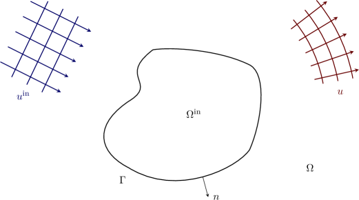
Figure 1: Visualisation of the scattering problem.

We study the situation depicted in Figure 1 where an incident wave $u^{\textup{in}}$ is scattered by the stationary obstacle $\Omega^{\textup{in}}$, causing a scattered wave $u$ to propagate in the free space $\Omega$. In the absence of external sources, we may assume that $u$ satisfies the homogeneous wave equation

$$\frac{\partial^{2}u}{\partial t^{2}}(x,t)-c^{2}\Delta u(x,t)=0,\quad(x,t)\in\Omega\times(0,T).$$ (1)

Here, the coefficient $c$ is the speed at which the wave travels in the medium. Using dimensionless units, we set $c=1$. Moreover, $\Delta$ is the Laplacian in the spatial domain and $T>0$ is a fixed final time. Depending on the characteristics of the scatterer $\Omega^{\textup{in}}$ and the incoming wave $u^{\textup{in}}$, the scattered wave $u$ is subject to boundary conditions posed on the surface $\Gamma$. We prescribe mixed boundary conditions of the form

$$u(x,t) =g_{D}(x,t), (x,t)\in\Gamma_{D}\times(0,T),$$ (2)

$$\frac{\partial u}{\partial n}(x,t) =g_{N}(x,t), (x,t)\in\Gamma_{N}\times(0,T),$$

given either on the Dirichlet boundary $\Gamma_{D}$ or the Neumann boundary $\Gamma_{N}$ with

$$\Gamma=\overline{\Gamma}_{D}\cup\overline{\Gamma}_{N},\quad\Gamma_{D}\cap\Gamma_{N}=\varnothing.$$

Furthermore, we assume that $u^{\textup{in}}$ has not reached $\Omega$ yet, which implies vanishing initial conditions for $u$,

$$u(x,0)=\frac{\partial u}{\partial t}(x,0)=0,\quad x\in\Omega.$$

Remark 1.

Surprisingly enough, regularity results for hyperbolic problems of type (1) with non-homogeneous boundary conditions were not available until the fundamental works of Lions and Magenes [43]. By the use of sophisticated tools from functional analysis and the theory of pseudo-differential operators, they paved the way for the mathematical analysis of general second-order hyperbolic systems. Subsequently, their findings were substantially improved and we present two examples here. Let $\Sigma=\Gamma\times[0,T]$ be the lateral boundary of the space-time cylinder $Q=\Omega\times[0,T]$. For the pure Dirichlet case, $\Gamma_{D}=\Gamma$, it is shown in [44] that

$$g_{D}\in H^{1}(\Sigma)\implies u\in C^{0}(H^{1}(\Omega);[0,T]),\ \frac{\partial}{\partial n}u\in L^{2}(\Sigma).$$

In comparison, optimal regularity results for the Neumann problem, $\Gamma=\Gamma_{N}$, are derived in [45] and are of the form

$$g_{N}\in L^{2}(\Sigma)\implies u\in H^{3/4}(Q),\ u_{|\Sigma}\in H^{1/2}(\Sigma).$$

In [46] it is shown that this result cannot be improved, i.e. that for all $\varepsilon>0$ there exist $g_{N}\in L^{2}(\Sigma)$ such that $u\not\in H^{3/4+\varepsilon}(Q)$. From these findings, it becomes evident that the situation of mixed conditions like (2) is far from trivial and needs special treatment. An alternative approach involves the theory of boundary integral equations, which are introduced in Section 2.2. In combination with the semi-group theory [3] or Laplace domain techniques [1, 2], general transmission problems can be treated in a uniform manner. To keep things simple, we refrain from specifying the function spaces in the following sections and refer to the given publications instead.

2.2 Boundary Integral Equations

The fundamental solution of (1) is given by

$$u^{\ast}(y-x,t-\tau)=\frac{\delta\left(t-\tau-\left\lvert y-x\right\rvert\right)}{4\pi\left\lvert y-x\right\rvert},\quad(x,t)\in\Omega\times(0,T),$$

where $\delta$ is the Dirac delta distribution defined by

$$\left(\delta(t-\tau-\left\lvert y-x\right\rvert)\right)(\varphi)=\varphi(t-\left\lvert y-x\right\rvert)$$

for smooth test functions $\varphi$. Thus, the behaviour of the wave at position $x$ and time $t$ is completely determined by its values at locations $y$ and earlier times $\tau=t-\left\lvert y-x\right\rvert$. In other words, an event at $(x,t)$ is only affected by actions that took place on the backward light cone

$$\left\{(y,\tau)\in\overline{Q}:\tau=t-\left\lvert y-x\right\rvert\right\}$$

of $(x,t)$ in space-time. Therefore, $u^{\ast}$ is also known as retarded Green’s function and $\tau=t-\left\lvert y-x\right\rvert$ is called retarded time [47]. This property becomes particularly important in the representation formula,

$$u(x,t) =-\int\limits_{0}^{t}\int\limits_{\Gamma}u^{\ast}(y-x,t-\tau)\,\frac{\partial}{\partial n}u(y,\tau)\mathop{dS(y)}\mathop{d\tau}$$ (3)

$$\hskip 51.6665pt+\int\limits_{0}^{t}\int\limits_{\Gamma}\frac{\partial u^{\ast}}{\partial n_{y}}(y-x,t-\tau)\,u(y,\tau)\mathop{dS(y)}\mathop{d\tau},$$

which expresses the solution by the convolution of the boundary data with the fundamental solution. Although formally specified on the lateral surface $\Sigma$, the evaluation of the Dirac delta reduces the domain of integration to its intersection with the backward light cone,

$$u(x,t) =-\int\limits_{\Gamma}\frac{1}{4\pi\left\lvert y-x\right\rvert}\frac{\partial}{\partial n}u(y,t-\left\lvert y-x\right\rvert)\mathop{dS(y)}\mathop{d\tau}$$ (4)

$$\hskip 25.83325pt+\int\limits_{\Gamma}\frac{(y-x)\cdot n_{y}}{4\pi\left\lvert y-x\right\rvert^{2}}\left(\frac{u(y,t-\left\lvert y-x\right\rvert)}{\left\lvert y-x\right\rvert}+\frac{\partial}{\partial t}u(y,t-\left\lvert y-x\right\rvert)\right)\mathop{dS(y)}\mathop{d\tau}.$$

Since the boundary data is only given on $\Gamma_{D}$ or $\Gamma_{N}$, we derive a system of boundary integral equations for its unknown parts. To this end, we define the trace operators $\gamma_{0}$ and $\gamma_{1}$ by

$$\gamma_{0,x}v(x)=\lim_{y\to x}v(y),\quad\gamma_{1,x}v(x)=\lim_{y\to x}\nabla v(y)\cdot n(x),\quad x\in\Gamma,\ y\in\Omega,$$

for sufficiently smooth $v$. Note that $\gamma_{1}$ coincides with the normal derivative $\partial/\partial n$. Now, we take the Dirichlet trace in (3) and obtain the first equation

$$\gamma_{0,x}u(x,t) =-\int\limits_{0}^{t}\int\limits_{\Gamma}u^{\ast}(y-x,t-\tau)\,\gamma_{1,y}u(y,\tau)\mathop{dS(y)}\mathop{d\tau}+\frac{1}{2}\gamma_{0,x}u(x,t)$$

$$\quad-\int\limits_{0}^{t}\int\limits_{\Gamma}\gamma_{1,y}u^{\ast}(y-x,t-\tau)\,\gamma_{0,y}u(y,\tau)\mathop{dS(y)}\mathop{d\tau}$$

for almost every $(x,t)\in\Sigma$. Similarly, the application of the Neumann trace yields

$$\gamma_{1,x}u(x,t) =\frac{1}{2}\gamma_{1,x}u(x,t)-\int\limits_{0}^{t}\int\limits_{\Gamma}\gamma_{1,x}u^{\ast}(y-x,t-\tau)\,\gamma_{1,x}u(y,\tau)\mathop{dS(y)}\mathop{d\tau}$$

$$\quad-\int\limits_{0}^{t}\int\limits_{\Gamma}\gamma_{1,x}\gamma_{1,y}\,u^{\ast}(y-x,t-\tau)\,u(y,\tau)\mathop{dS(y)}\mathop{d\tau}.$$

We identify the terms above with so-called boundary integral operators,

$$\left(\mathcal{V}w\right)(x,t) =\int\limits_{0}^{t}\int\limits_{\Gamma}u^{\ast}(y-x,t-\tau)\,w(y,\tau)\mathop{dS(y)}\mathop{d\tau},$$ (5)

$$\left(\mathcal{K}w\right)(x,t) =\int\limits_{0}^{t}\int\limits_{\Gamma}\gamma_{1,y}u^{\ast}(y-x,t-\tau)\,w(y,\tau)\mathop{dS(y)}\mathop{d\tau},$$

$$\left(\mathcal{K}^{\prime}w\right)(x,t) =\int\limits_{0}^{t}\int\limits_{\Gamma}\gamma_{1,x}u^{\ast}(y-x,t-\tau)\,w(y,\tau)\mathop{dS(y)}\mathop{d\tau},$$

$$\left(\mathcal{D}w\right)(x,t) =\int\limits_{0}^{t}\int\limits_{\Gamma}\gamma_{1,x}\gamma_{1,y}u^{\ast}(y-x,t-\tau)\,w(y,\tau)\mathop{dS(y)}\mathop{d\tau},$$

$$\left(\mathcal{I}w\right)(x,t) =\int\limits_{0}^{t}\int\limits_{\Gamma}\delta(t-\tau-\left\lvert y-x\right\rvert)\,w(y,\tau)\mathop{dS(y)}\mathop{d\tau},$$

and rewrite the boundary integral equations in matrix form,

$$\begin{pmatrix}\gamma_{0,x}u\\ \gamma_{1,x}u\end{pmatrix}(x,t)=\left[\begin{pmatrix}\tfrac{1}{2}\mathcal{I}+\mathcal{K}&-\mathcal{V}\\ -\mathcal{D}&\tfrac{1}{2}\mathcal{I}-\mathcal{K}^{\prime}\end{pmatrix}\begin{pmatrix}\gamma_{0,y}u\\ \gamma_{1,y}u\end{pmatrix}\right](x,t),\quad(x,t)\in\Sigma.$$ (6)

Hence, the solution to the wave equation (1) is found by solving for the unknown boundary data in the system above and inserting it into the representation formula (3). For the mapping properties of the operators and the solvability of the equations, we refer to [3].

2.3 Galerkin formulation

We derive a Galerkin formulation of (6). Taking mixed boundary conditions (2) into account, we choose extensions $\tilde{g}_{D}$ and $\tilde{g}_{N}$ on $\Gamma$ satisfying

$$\tilde{g}_{D}(x,t)=g_{D}(x,t),\ x\in\Gamma_{D},\quad\tilde{g}_{N}(x,t)=g_{N}(x,t),\ x\in\Gamma_{N},\quad t\in[0,T].$$

Furthermore, we decompose the Dirichlet and Neumann traces as follows

$$\gamma_{0}u =\tilde{u}+\tilde{g}_{D} \tilde{u}(x,t)=0 \textup{ for }(x,t)\in\Gamma_{D}\times[0,T],$$ with

$$\gamma_{1}u =\tilde{q}+\tilde{g}_{N} \tilde{q}(x,t)=0 \textup{ for }(x,t)\in\Gamma_{N}\times[0,T],$$ with

and obtain for $t\in[0,T]$

$$\left(\mathcal{V}\tilde{q}\right)(x,t)-\left(\mathcal{K}\tilde{u}\right)(x,t) =\left[\Bigl{(}-\tfrac{1}{2}\mathcal{I}+\mathcal{K}\Bigr{)}\tilde{g}_{D}\right](x,t)-\left(\mathcal{V}\tilde{g}_{N}\right)(x,t), x\in\Gamma_{D},$$

$$\left(\mathcal{K}^{\prime}\tilde{q}\right)(x,t)+\left(\mathcal{D}\tilde{u}\right)(x,t) =\left[\Bigl{(}-\tfrac{1}{2}\mathcal{I}-\mathcal{K}^{\prime}\Bigr{)}\tilde{g}_{N}\right](x,t)-\left(\mathcal{D}\tilde{g}_{D}\right)(x,t), x\in\Gamma_{N}.$$

Here, the right hand side is known and we have to solve for the unknown Neumann data $\tilde{q}$ on the Dirichlet boundary $\Gamma_{D}$ and the Dirichlet data $\tilde{u}$ on the Neumann part $\Gamma_{N}$, respectively. Hence, the Galerkin formulation is to find $\tilde{q}$ and $\tilde{u}$ such that

$$\left\langle w,\mathcal{V}\tilde{q}\right\rangle_{\Gamma_{D}}-\left\langle w,\mathcal{K}\tilde{u}\right\rangle_{\Gamma_{D}} =\left\langle w,\left(-\tfrac{1}{2}\mathcal{I}+\mathcal{K}\right)\tilde{g}_{D}\right\rangle_{\Gamma_{D}}-\left\langle w,\mathcal{V}\tilde{g}_{N}\right\rangle_{\Gamma_{D}},$$ (7)

$$\left\langle v,\mathcal{K}^{\prime}\tilde{q}\right\rangle_{\Gamma_{N}}+\left\langle v,\mathcal{D}\tilde{u}\right\rangle_{\Gamma_{N}} =\left\langle v,\left(-\tfrac{1}{2}\mathcal{I}-\mathcal{K}^{\prime}\right)\tilde{g}_{N}\right\rangle_{\Gamma_{N}}-\left\langle v,\mathcal{D}\tilde{g}_{D}\right\rangle_{\Gamma_{N}}$$

holds at every time $t\in[0,T]$ and for all test functions $w$ and $v$. The index of the duality product $\left\langle\cdot,\cdot\right\rangle$ indicates on which part of the boundary it is formed.

3 Numerical Discretisation

In view of the numerical treatment of (7), we have to discretise both time and space. We start with the time discretisation.

3.1 Convolution Quadrature Method

The application of the integral operators in (5) requires the evaluation of the convolution in time of the form

$$h(t)=\int\limits_{0}^{t}f(t-\tau)g(\tau)\mathop{d\tau},\quad 0\leq t\leq T,$$ (8)

where $f$ is a distribution and $g$ is smooth. In order to compute such convolutions numerically, we employ the Convolution Quadrature Method (CQM) introduced in [13]. It is based on the Fourier-Laplace transform defined by

$$\hat{f}(s)=\int\limits_{0}^{\infty}f(t)e^{-st}\mathop{dt}\in\mathbb{C},\quad s\in\mathbb{C},$$

and on the observation that we can replace $f$ by the inverse transform of $\hat{f}$ and change the order of integration, i.e.

$$h(t)=\int\limits_{\mathcal{C}}\int\limits_{0}^{t}e^{(t-\tau)s}g(\tau)\mathop{d\tau}\hat{f}(s)\mathop{ds},\quad 0\leq t\leq T.$$

The integration is performed along the contour

$$\mathcal{C}=\left\{s\in\mathbb{C}:\sigma+\imath z,\ z\in\mathbb{R}\right\},$$

where $\sigma>0$ is greater than the real part of all singularities of $\hat{f}$. In further steps, the inner integral is approximated by a linear multi-step method and Cauchy’s integral formula is used. In this way, the CQM yields approximations of (8) at discrete time points

$$t_{n}=n\Delta t,\quad\Delta t=T/N,\quad n=0,\ldots,N,$$

via the quadrature formula

$$h(t_{n})\approx\sum_{k=0}^{n}\omega_{n-k}\,g(t_{k}),\quad n=0,\ldots,N.$$ (9)

For a parameter $R>0$, the quadrature weights are defined by

$$\omega_{n}=\frac{R^{-n}}{N}\sum_{\ell=0}^{N-1}\hat{f}\left(s_{\ell}\right)e^{\tfrac{-2\pi\imath}{N}n\ell},\quad n=0,\ldots,N,$$ (10)

and they are given in terms of $\hat{f}$ sampled at specific frequencies

$$s_{\ell}=\frac{\chi\left(R\cdot e^{\tfrac{2\pi\imath}{N}\ell}\right)}{\Delta t}\in\mathbb{C},\quad\ell=0,\ldots,N-1,$$ (11)

which depend on the characteristic function $\chi$ of the multi-step method [48]. For the choice of the parameter $R$ and further details we refer the reader to [13, 14, 15].

Returning to the setting of (7), we apply the CQM to approximate the expressions occurring in the Galerkin formulation, for instance $h(t)=\left\langle w,\mathcal{V}\tilde{q}(t)\right\rangle_{\Gamma_{D}}$, at equidistant time steps $t=t_{n}$. For the the single layer operator $\mathcal{V}$ we obtain

$$\left\langle w,\mathcal{V}\tilde{q}(t_{n})\right\rangle_{\Gamma_{D}} =\int\limits_{0}^{t_{n}}\int\limits_{\Gamma_{D}}\int\limits_{\Gamma}u^{\ast}(y-x,t_{n}-\tau)\,\tilde{q}(y,\tau)\mathop{dS(y)}w(x)\mathop{dS(x)}\mathop{d\tau}$$

$$\approx\int\limits_{\Gamma_{D}}\int\limits_{\Gamma}\sum_{k=0}^{n}\omega_{n-k}(y-x)\,\tilde{q}(y,t_{k})\mathop{dS(y)}w(x)\mathop{dS(x)},$$

with quadrature weights

$$\omega_{n-k}(y-x)=\frac{R^{-(n-k)}}{N}\sum_{\ell=0}^{N-1}\hat{u}^{\ast}\left(y-x,s_{\ell}\right)e^{\tfrac{-2\pi\imath}{N}(n-k)\ell}.$$

The transformed fundamental solution $\hat{u}^{\ast}$ is precisely the fundamental solution of the Helmholtz equation for complex frequencies $s\in\mathbb{C}$,

$$-\Delta\hat{u}+s^{2}\hat{u}=0,$$

and has the representation

$$\hat{u}^{\ast}(y-x,s)=\frac{e^{\textstyle{-s\left\lvert y-x\right\rvert}}}{4\pi\left\lvert y-x\right\rvert}.$$ (12)

In contrast to the retarded fundamental solution $u^{\ast}$, its transform $\hat{u}^{\ast}$ defines a smooth function for $x\neq y$ and all $s$. Hence, the CQM formulation has the advantage that distributional kernel functions are avoided. We set $\tilde{q}_{k}=\tilde{q}(\cdot,t_{k})$ and introduce the operator

$$\widehat{\mathbf{V}}_{n-k}\,\tilde{q}_{k}(x)=\frac{R^{-(n-k)}}{N}\sum_{\ell=0}^{N-1}e^{\tfrac{-2\pi\imath}{N}(n-k)\ell}\int\limits_{\Gamma}\hat{u}^{\ast}\left(y-x,s_{\ell}\right)\tilde{q}_{k}(y)\mathop{dS(y)},$$ (13)

which acts only on the spatial component. Finally, we end up with the approximation

$$\left\langle w,\mathcal{V}\tilde{q}(t_{n})\right\rangle_{\Gamma_{D}}\approx\sum_{k=0}^{n}\left\langle w,\widehat{\mathbf{V}}_{n-k}\,\tilde{q}_{k}\right\rangle_{\Gamma_{D}},$$

where the continuous convolution is now replaced by a discrete one. Repeating this procedure for the other integral operators leads to the time-discretised Galerkin formulation: find $\tilde{u}_{k}$ and $\tilde{q_{k}}$, $k=0,\ldots,N$, such that

$$\sum_{k=0}^{n}\left(\begin{aligned} \left\langle w,\widehat{\mathbf{V}}_{n-k}\,\tilde{q}_{k}\right\rangle_{\Gamma_{D}}-\left\langle w,\widehat{\mathbf{K}}_{n-k}\,\tilde{u}_{k}\right\rangle_{\Gamma_{D}}\\ \left\langle v,\widehat{\mathbf{K}}^{\prime}_{n-k}\,\tilde{q}_{k}\right\rangle_{\Gamma_{N}}+\left\langle v,\widehat{\mathbf{D}}_{n-k}\,\tilde{u}_{k}\right\rangle_{\Gamma_{N}}\end{aligned}\right) =$$ (14)

$$\sum_{k=0}^{n}\left(\begin{aligned} \left\langle w,\left(-\tfrac{1}{2}\widehat{\mathbf{I}}_{n-k}+\widehat{\mathbf{K}}_{n-k}\right)\tilde{g}_{D,k}\right\rangle_{\Gamma_{D}}-\left\langle w,\widehat{\mathbf{V}}_{n-k}\,\tilde{g}_{N,k}\right\rangle_{\Gamma_{D}}\\ \left\langle v,\left(-\tfrac{1}{2}\widehat{\mathbf{I}}_{n-k}-\widehat{\mathbf{K}}^{\prime}_{n-k}\right)\tilde{g}_{N,k}\right\rangle_{\Gamma_{N}}-\left\langle v,\widehat{\mathbf{D}}_{n-k}\tilde{g}_{D,k}\right\rangle_{\Gamma_{N}}\end{aligned}\right)$$

holds for all test functions $w$ and $v$ and $n=0,\ldots,N$.

From its Definition (13), we see that the single layer operator $\widehat{\mathbf{V}}_{n-k}$ admits the representation

$$\widehat{\mathbf{V}}_{n-k}\,\tilde{q}_{k}(x)=\frac{R^{-(n-k)}}{N}\sum_{\ell=0}^{N-1}e^{\tfrac{-2\pi\imath}{N}(n-k)\ell}\left(\mathbf{V}_{\ell}\,\tilde{q}_{k}\right)(x)$$ (15)

as a scaled discrete Fourier transform of operators $\mathbf{V}_{\ell}$,

$$\mathbf{V}_{\ell}\,\tilde{q}_{k}(x)=\int\limits_{\Gamma}\hat{u}^{\ast}\left(y-x,s_{\ell}\right)\tilde{q}_{k}(y)\mathop{dS(y)},\quad\ell=0,\ldots,N-1.$$

These are exactly the single layer operators corresponding to the Helmholtz equations with frequencies $s_{\ell}$. In the same manner, the other integral operators $\widehat{\mathbf{K}}_{n-k}$, $\widehat{\mathbf{K}}^{\prime}_{n-k}$ and $\widehat{\mathbf{D}}_{n-k}$ may be written in terms of the respective operators $\mathbf{K}_{\ell}$, $\mathbf{K}_{\ell}^{\prime}$, $\mathbf{D}_{\ell}$ of the Helmholtz equations. Since $\textup{Im}(s_{\ell})\neq 0$, the single layer operator $\mathbf{V}_{\ell}$ and hypersingular operator $\mathbf{D}_{\ell}$ are elliptic [49, 1]. The operator $\widehat{\mathcal{I}}_{n-k}$ on the other hand can be easily calculated,

$$\widehat{\mathbf{I}}_{0}=\mathcal{I},\quad\widehat{\mathbf{I}}_{n-k}=0,\quad k\neq n.$$

Therefore, the spatial discretisation of (14) is equivalent to a spatial discretisation of a sequence of Helmholtz problems.

3.2 Galerkin Approximation

We assume that the boundary $\Gamma$ admits a decomposition into flat triangular elements, which belong either to $\Gamma_{D}$ or $\Gamma_{N}$. We define boundary element spaces of constant and linear order

$$S_{h}^{0}(\Gamma_{D})=\operatorname{span}{\left\{\varphi_{m}^{0}\right\}}_{m=1}^{M_{D}},\quad S_{h}^{1}(\Gamma_{N})=\operatorname{span}{\left\{\varphi_{m}^{1}\right\}}_{m=1}^{M_{N}},$$

and global variants

$$S_{h}^{0}(\Gamma)=\operatorname{span}{\left\{\varphi_{m}^{0}\right\}}_{m=1}^{M_{0}},\quad S_{h}^{1}(\Gamma)=\operatorname{span}{\left\{\varphi_{m}^{1}\right\}}_{m=1}^{M_{1}}.$$

Then, we follow the ansatz

$$\tilde{q}_{n}=\sum_{m=1}^{M_{D}}\underline{q}_{n}[m]\,\varphi_{m}^{0}\in S_{h}^{0}(\Gamma_{D}),\quad\tilde{u}_{n}=\sum_{m=1}^{M_{N}}\underline{u}_{n}[m]\,\varphi_{m}^{1}\in S_{h}^{1}(\Gamma_{N}),\quad n=0,\ldots,N,$$

with $\underline{q}_{n}\in\mathbb{R}^{M_{D}}$, $\underline{u}_{n}\in\mathbb{R}^{M_{N}}$ to approximate the unknown Neumann and Dirichlet data. Likewise, the boundary conditions are represented by coefficient vectors $\underline{g}_{n}^{N}\in\mathbb{R}^{M_{0}}$ and $\underline{g}_{n}^{D}\in\mathbb{R}^{M_{1}}$, which are determined by $L^{2}$-projections onto $S_{h}^{i}(\Gamma)$.

As pointed out before, we begin with the discretisation of the boundary integral operators of Helmholtz problems. For each frequency $s_{\ell}$, $\ell=0,\ldots,N-1$, we have boundary element matrices

$$\begin{gathered}V_{\ell}\in\mathbb{C}^{M_{D}\times M_{0}},\quad K_{\ell}\in\mathbb{C}^{M_{D}\times M_{1}},\quad K^{\prime}_{\ell}\in\mathbb{C}^{M_{N}\times M_{0}},\quad D_{\ell}\in\mathbb{C}^{M_{N}\times M_{1}},\\ I\in\mathbb{R}^{M_{D}\times M_{1}},\quad I^{\prime}\in\mathbb{R}^{M_{N}\times M_{0}},\end{gathered}$$

defined by

$$V_{\ell}[m,i] =\left\langle\varphi_{m}^{0},\mathbf{V}_{\ell}\varphi_{i}^{0}\right\rangle_{\Gamma_{D}}, K_{\ell}[m,j] =\left\langle\varphi_{m}^{0},\mathbf{K}_{\ell}\varphi_{j}^{1}\right\rangle_{\Gamma_{D}},$$

$$K^{\prime}_{\ell}[p,i] =\left\langle\varphi_{p}^{1},\mathbf{K}^{\prime}_{\ell}\varphi_{i}^{0}\right\rangle_{\Gamma_{N}}, D_{\ell}[p,j] =\left\langle\varphi_{p}^{1},\mathbf{D}_{\ell}\varphi_{j}^{1}\right\rangle_{\Gamma_{N}},$$

$$I[m,j] =\left\langle\varphi_{m}^{0},\varphi_{j}^{1}\right\rangle_{\Gamma_{D}}, I^{\prime}[p,i] =\left\langle\varphi_{p}^{1},\varphi_{i}^{0}\right\rangle_{\Gamma_{N}},$$

with $i=1,\ldots,M_{0}$, $j=1,\ldots,M_{1}$, $m=1,\ldots,M_{D}$, $p=1,\ldots,M_{N}$. Just as in (15), these auxiliary matrices are then transformed to obtain the integration weights of the CQM. In the case of the single layer operators this amounts to

$$\widehat{V}_{n}=\frac{R^{-n}}{N}\sum_{\ell=0}^{N-1}e^{\tfrac{-2\pi\imath}{L}n\ell}\ V_{\ell},\quad n=0,\ldots,N,$$ (16)

such that

$$\widehat{V}_{n}[m,i]=\left\langle\varphi_{m}^{0},\widehat{\mathbf{V}}_{n}\varphi_{i}^{0}\right\rangle_{\Gamma_{D}},\quad i=1,\ldots,M_{0},\quad m=1,\ldots,M_{D},$$

holds by linearity. Moreover, we identify sub-matrices

$$\widehat{V}^{D}_{n} =\widehat{V}_{n}[1:M_{D},1:M_{D}]\in\mathbb{C}^{M_{D}\times M_{D}},$$

$$\widehat{K}^{N}_{n} =\widehat{K}_{n}[1:M_{D},1:M_{N}]\in\mathbb{C}^{M_{D}\times M_{N}},$$

$$\widehat{D}^{N}_{n} =\widehat{D}_{n}[1:M_{N},1:M_{N}]\in\mathbb{C}^{M_{N}\times M_{N}}.$$

The Galerkin approximation of (14) is then equivalent to the system of linear equations

$$\begin{pmatrix}\widehat{V}^{D}_{0}&-\widehat{K}^{N}_{0}\\[4.30554pt] (\widehat{K}^{N}_{0})^{\top}&\widehat{D}^{N}_{0}\end{pmatrix}\begin{pmatrix}\underline{q}_{n}\\[4.30554pt] \underline{u}_{n}\end{pmatrix}=\begin{pmatrix}f_{n}^{D}\\[4.30554pt] f_{n}^{N}\end{pmatrix},\quad n=0,\ldots,N,$$ (17)

with right-hand side

$$\begin{pmatrix}f_{n}^{D}\\[4.30554pt] f_{n}^{N}\end{pmatrix} =-\frac{1}{2}\begin{pmatrix}I\underline{g}_{n}^{D}\\[4.30554pt] I^{\prime}\underline{g}_{n}^{N}\end{pmatrix}+\sum_{k=0}^{n}\begin{pmatrix}-\widehat{V}_{n-k}&\widehat{K}_{n-k}\\[4.30554pt] -\widehat{K}^{\prime}_{n-k}&-\widehat{D}_{n-k}\end{pmatrix}\begin{pmatrix}\underline{g}_{k}^{N}\\[4.30554pt] \underline{g}_{k}^{D}\end{pmatrix}$$ (18)

$$\hskip 86.11084pt+\sum_{k=0}^{n-1}\begin{pmatrix}-\widehat{V}^{D}_{n-k}&\widehat{K}^{N}_{n-k}\\[4.30554pt] -(\widehat{K}^{N}_{n-k})^{\top}&-\widehat{D}^{N}_{n-k}\end{pmatrix}\begin{pmatrix}\underline{q}_{k}\\[4.30554pt] \underline{u}_{k}\end{pmatrix}.$$

While the first row in (18) corresponds to the right-hand side of (14), the second row contains the boundary values of the previous time steps and results from the convolutional structure of the CQM approximation. Since the left-hand side of the linear system stays the same for every time step, only one matrix inversion has to be performed throughout the whole simulation. To be more precise, system (17) is equivalent to the decoupled system

$$S\underline{u}_{n} =f_{n}^{N}-(\widehat{K}^{N}_{0})^{\top}(\widehat{V}^{D}_{0})^{-1}f_{n}^{D},$$

$$\widehat{V}^{D}_{0}\underline{q}_{n} =\widehat{K}^{N}_{0}\underline{u}_{n}+f_{n}^{D},$$

where $S$ is the Schur complement

$$S=\widehat{D}^{N}_{0}+(\widehat{K}^{N}_{0})^{\top}(\widehat{V}^{D}_{0})^{-1}\widehat{K}^{N}_{0}.$$

Since both $\widehat{V}_{0}$ and $S$ are real symmetric and positive definite, we factorise them via LU decomposition once for $n=0$ and use forward and backward substitution to solve the systems progressively in time.

Naturally, the assembly of the boundary element matrices and the computation of the right-hand side (18) for each step are the most demanding parts of the algorithm, both computational and storage wise. Due to the fact that the matrices are generally fully populated, sparse approximation techniques are indispensable for large scale problems. Compared to stationary problems, this is even more crucial here, as the amount of numerical work scales with the number of time steps. Therefore, it is necessary to not only approximate in the spatial but also in the frequency variable. It proves to be beneficial to interpret the array of matrices $V_{k}$, $k=0,\ldots,N-1$, as a third order tensor

$$\boldsymbol{\mathcal{V}}[i,j,k]=V_{k}[i,j].$$ (19)

In this way, we can restate the problem within the frame of general tensor approximation and compression. To that end, we introduce low-rank factorisations which make use of the tensor product.

Definition 1 (Tensor Product).

For matrices $A^{(j)}\in\mathbb{C}^{r_{j}\times I_{j}}$, $j=1,\ldots,d$ and a tensor $\boldsymbol{\mathcal{X}}\in\mathbb{C}^{I_{1}\times\cdots\times I_{d}}$, we define the tensor or mode product $\times_{j}$ by

$$\left(\boldsymbol{\mathcal{X}}\times_{j}A^{(j)}\right)[i_{1},\ldots,i_{j-1},\ell,i_{j+1},\ldots,i_{d}]=\sum_{i_{j}=1}^{I_{j}}\boldsymbol{\mathcal{X}}[i_{1},\ldots,i_{d}]\,A^{(j)}[\ell,i_{j}],\quad\ell=1,\ldots,r_{j}.$$

Because of the singular nature of the fundamental solution, a global low-rank approximation of $\boldsymbol{\mathcal{V}}$ is practically not achievable. Instead, we follow a hierarchical approach where we partition the tensor into blocks, which we approximate individually. Our scheme is based on $\mathcal{H}^{2}$-matrix approximation in the spatial domain, i.e. in $i$ and $j$, and ACA in the frequency, i.e. in $k$.

4 Hierarchical Matrices

The boundary element matrices $V_{k}$ are of the form

$$G[i,j]=\int\limits_{\Gamma}\int\limits_{\Gamma}g(x,y)\varphi_{j}(y)\mathop{dS(y)}\psi_{i}(x)\mathop{dS(x)},\quad i\in I,j\in J,$$

where $\psi_{i}$ and $\varphi_{j}$ are trial and test functions respectively with index sets $I$ and $J$ and $g$ is a kernel function. We associate with each $i\in I$ and $j\in J$ sets $X_{i}$ and $Y_{j}$, which correspond to the support of the trial and test functions $\psi_{i}$ and $\varphi_{j}$. For $r\subset I$ and $c\subset J$, we define

$$X_{r}=\bigcup_{i\in r}\,X_{i}\textup{ and }Y_{c}=\bigcup_{j\in c}\,Y_{j}.$$

Moreover, we choose axis-parallel boxes $B_{r}$ and $B_{c}$ that contain the sets $X_{r}$ and $Y_{c}$, respectively.

Since $g$ is non-local, the matrix $G$ is typically fully populated. However, if $X_{r}$ and $Y_{c}$ are well separated, i.e. if they satisfy the admissibility condition

$$\max\left\{\operatorname{diam}(X_{r}),\operatorname{diam}(X_{c})\right\}\leq\eta\operatorname{dist}(X_{r},X_{c})$$ (20)

for fixed $\eta>0$, then the kernel function admits the degenerated expansion

$$g(x,y)\approx\sum_{\mu=1}^{p}\sum_{\nu=1}^{p}L_{r,\mu}(x)g(\xi_{r,\mu},\xi_{c,\nu})L_{c,\nu}(y),\quad x\in X_{r},y\in Y_{c},$$ (21)

into Lagrange polynomials $L_{r,\mu}$ and $L_{c,\nu}$ on $X_{r}\times Y_{c}$ . Here, we choose tensor products $\xi_{r,\mu}$ and $\xi_{c,\nu}$ of Chebyshev points in $B_{r}$ and $B_{c}$ as interpolation points. In doing so, the double integral reduces to a product of single integrals

$$G[i,j]\approx\sum_{\mu=1}^{p}\sum_{\nu=1}^{p}g(\xi_{r,\mu},\xi_{c,\nu})\int\limits_{\Gamma}L_{r,\mu}(x)\psi_{i}(x)\mathop{dS(x)}\int\limits_{\Gamma}L_{c,\nu}(y)\varphi_{j}(y)\mathop{dS(y)},\ (i,j)\in r\times c,$$

which results in the low-rank approximation of the sub-block

$$G[b]\approx U_{b}\,S_{b}\,W_{b}^{H},\quad b=r\times c,$$ (22)

with

$$U_{b}[i,\mu] =\int\limits_{\Gamma}L_{r,\mu}(x)\psi_{i}(x)\mathop{dS(x)}, i\in r,\quad\mu=1,\ldots,p,$$

$$S_{b}[\mu,\nu] =g(\xi_{r,\mu},\xi_{c,\nu}), \mu,\nu=1,\ldots,p,$$

$$W_{b}[j,\nu] =\int\limits_{\Gamma}L_{c,\nu}(y)\varphi_{j}(y)\mathop{dS(y)}, j\in c,\quad\nu=1,\ldots,p.$$

By approximating suitable sub-blocks with low-rank matrices, we obtain a hierarchical matrix approximation of $G$. This approach leads to a reduction of both computational and storage costs for assembling $G$ from quadratic to almost linear in $\#I$ and $\#J$, where $\#I$ denotes the cardinality of the set $I$.

4.1 Matrix Partitions

In the following, we give a short introduction on hierarchical matrices based on the monographs [30, 50]. Since only sub-blocks that satisfy the admissibility condition (20) permit accurate low-rank approximations, a partition of the matrix indices $I\times J$ into admissible and inadmissible blocks is required. To this end, we define cluster trees for $I$ and $J$.

Definition 2 (Cluster trees).

Let $\mathcal{T}(I)$ be a tree with nodes $\varnothing\neq r\subset I$. We call $\mathcal{T}(I)$ a cluster tree if the following conditions hold:

1. $I$ is the root of $\mathcal{T}(I)$.

2. If $r\in\mathcal{T}(I)$ is not a leaf, then $r$ is the disjoint union of its sons

   $$r=\bigcup_{r^{\prime}\in\operatorname{sons}(r)}r^{\prime}.$$

3. $\#\operatorname{sons}(r)\neq 1$ for $r\in\mathcal{T}(I)$.

We denote by $\mathcal{L}(\mathcal{T}(I))$ the set of leaf clusters

$$\mathcal{L}(\mathcal{T}(I))=\left\{r\in\mathcal{T}(I):\operatorname{sons}(r)=\varnothing\right\}.$$

Moreover, we assume that the size of the clusters is bounded from below, i.e.

$$\#r>n_{\min}>1,\quad r\in\mathcal{T}(I),$$

in order to control the number of clusters and limit the overhead in practical applications.

There are several strategies to perform the clustering efficiently. For instance, the geometric clustering in [32] constructs the cluster tree recursively by splitting the bounding box in the direction with largest extent. Alternatively, the principal component analysis can be used to produce well-balanced cluster trees [30].

Since searching the whole index set $I\times J$ for an optimal partition is not reasonable, we restrict ourselves to partitions which are based on cluster trees of $I$ and $J$.

Definition 3 (Block cluster trees).

Let $\mathcal{T}(I)$ and $\mathcal{T}(J)$ be cluster trees. We construct the block cluster tree $\mathcal{T}(I\times J)$ by

1. setting $I\times J$ as the root of $\mathcal{T}(I\times J)$,

2. and defining the sons recursively starting with $r\times c$ for $r=I$ and $c=J$:

   $$\operatorname{sons}(r\times c)=\left\{\begin{aligned} &\operatorname{sons}(r)\times c,&&\textup{if}\operatorname{sons}(r)\neq\varnothing\textup{ and }\operatorname{sons}(c)=\varnothing,\\ &r\times\operatorname{sons}(c),&&\textup{if}\operatorname{sons}(r)=\varnothing\textup{ and }\operatorname{sons}(c)\neq\varnothing,\\ &\operatorname{sons}(r)\times\operatorname{sons}(c),&&\textup{if}\operatorname{sons}(r)\neq\varnothing\textup{ and }\operatorname{sons}(c)\neq\varnothing,\\ &\varnothing,&&\textup{if }r\times c\textup{ is admissible or}\\ &&&\operatorname{sons}(r)=\operatorname{sons}(c)=\varnothing.\end{aligned}\right.$$

Then, the set of leaves $\mathcal{L}(\mathcal{T}(I\times J))$ is a partition in the following sense.

Definition 4 (Admissible partition).

We call $\mathcal{P}$ a partition of $I\times J$ with respect to the block cluster tree $\mathcal{T}(I\times J)$ if

1. $\mathcal{P}\subset\mathcal{T}(I\times J)$,

2. $b,b^{\prime}\in\mathcal{P}\implies b\cap b^{\prime}=\varnothing\textup{ or }b=b^{\prime}$,

3. $\dot{\bigcup}_{b\in\mathcal{P}}\,b=I\times J$.

Moreover, $\mathcal{P}$ is said to be admissible if every $r\times c\in\mathcal{P}$ is either admissible (20) or

$$\max\left\{\#r,\#c\right\}\leq n_{\min}.$$

In this case, the near and far field of $\mathcal{P}$ are defined by

$$\mathcal{P}^{-}=\left\{r\times c\in\mathcal{P}:\max\left\{\#r,\#c\right\}\leq n_{\min}\right\},\quad\mathcal{P}^{+}=\mathcal{P}\setminus\mathcal{P}^{-}.$$

Thus, the near field $\mathcal{P}^{-}$ describes those blocks of $G$ that are stored in full, because they are inadmissible or simply too small. On the other hand, the far field $\mathcal{P}^{+}$ contains admissible blocks only, which are approximated by low-rank matrices. In Figure 2 a partition for the single layer potential is visualised.

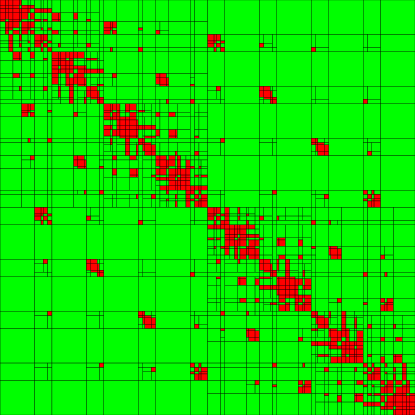
Figure 2: Visualisation of a matrix partition. Green blocks are admissible, whereas red ones are inadmissible.

Remark 2.

Since evaluating the admissibility condition (20) is rather expensive, we use the alternative condition

$$\max\left\{\operatorname{diam}(B_{r}),\operatorname{diam}(B_{c})\right\}\leq\eta\operatorname{dist}(B_{r},B_{s}),$$ (23)

which operates on the bounding boxes and is easier to check.

4.2 $\mathcal{H}^{2}$-matrices

One special class of hierarchical matrices consists of $\mathcal{H}^{2}$-matrices. They are based on the observation that the matrices $U_{b}$ and $W_{b}$ in the low-rank factorisation (22) of the far field block $b=r\times c$ only depend on the respective row cluster $r$ or column cluster $c$ and not on the block $b$ itself.

Definition 5 ($\mathcal{H}^{2}$-matrices).

Let $\mathcal{P}$ be an admissible partition of $I\times J$.

1. We call

   $${\left(U_{r}\right)}_{r\in\mathcal{T}(I)},\quad U_{r}\in\mathbb{C}^{r\times k_{r}},\quad k_{r}>0,$$

   (nested) cluster basis, if for all non-leaves $r\in\mathcal{T}(I)\setminus\mathcal{L}(\mathcal{T}(I))$ transfer matrices

   $$E_{r^{\prime},r}\in\mathbb{C}^{k_{r^{\prime}}\times k_{r}},\quad r^{\prime}\in\operatorname{sons}(r),\$$

   exist such that

   $$U_{r}=\begin{pmatrix}U_{r_{1}}E_{r_{1},r}\\ \dots\\ U_{r_{p}}E_{r_{p},r}\end{pmatrix},\quad\operatorname{sons}(r)=\left\{r_{1},\ldots,r_{p}\right\}.$$

2. $G$ is called $\mathcal{H}^{2}$-matrix with row cluster basis ${\left(U_{r}\right)}_{r\in\mathcal{T}(I)}$ and column cluster basis ${\left(W_{c}\right)}_{c\in\mathcal{T}(J)}$, if for each far field block $b=r\times c$ there are coupling matrices $S_{b}\in\mathbb{C}^{k_{r}\times k_{c}}$ such that

   $$G[b]=U_{r}\,S_{b}\,W_{c}^{H}.$$

In view of our interpolation scheme, we observe that the Lagrange polynomials of the father cluster $r\in\mathcal{T}(I)$ can be expressed by the Lagrange polynomials of its son clusters $r^{\prime}\in\operatorname{sons}(r)$ via interpolation,

$${L_{r,\mu}}(x)=\sum_{\lambda=1}^{p}L_{r,\mu}(\xi_{r^{\prime},\lambda})L_{r^{\prime},\lambda}(x),\quad x\in B_{r^{\prime}}.$$

Hence, by choosing transfer matrices

$$E_{r^{\prime},r}[\lambda,\mu]=L_{r,\mu}(\xi_{r^{\prime},\lambda}),$$

the cluster basis becomes nested

$$U_{r}[i,\mu] =\int\limits_{X_{i}}L_{r,\mu}(x)\psi_{i}(x)\mathop{dS(x)}=\sum_{\lambda=1}^{p}L_{r,\mu}(\xi_{r^{\prime},\lambda})\int\limits_{X_{i}}L_{r^{\prime},\lambda}(x)\psi_{i}(x)\mathop{dS(x)}$$

$$=\sum_{\lambda=1}^{p}E_{r^{\prime},r}[\lambda,\mu]\ U_{r^{\prime}}[i,\lambda]=\left(U_{r^{\prime}}E_{r^{\prime},r}\right)[i,\mu],\quad i\in r^{\prime}.$$

Algorithm 1 describes the assembly of cluster bases and summarises the construction of an $\mathcal{H}^{2}$ -matrix by interpolation.

In the following, let $\widetilde{G}$ be the $\mathcal{H}^{2}$-approximation of the dense Galerkin matrix $G$. Kernel functions like (12) are asymptotically smooth, i.e. there exist constants $C_{as}(\alpha,\beta)$ such that

$$\left\lvert\partial_{x}^{\alpha}\partial_{y}^{\beta}g(x,y)\right\rvert\leq C_{as}(\alpha,\beta)\left\lvert x-y\right\rvert^{-\left\lvert\alpha\right\rvert-\left\lvert\beta\right\rvert}\left\lvert g(x,y)\right\rvert,\quad x\neq y,$$ (24)

for all multi-indices $\alpha,\beta\in\mathbb{N}^{3}$. Together with the admissibility condition (23), this property implies exponential decay of the approximation error [50].

Theorem 1 (Approximation error).

Let $r\times c\in\mathcal{P}^{+}$ be admissible with $\eta\in(0,2)$ and let $g(\cdot,\cdot)$ be an asymptotically smooth function. If we use a fixed number of $m$ interpolation points in each direction, resulting in $p=m^{3}$ points overall, the separable approximation

$$\tilde{g}(x,y)=\sum_{\mu=1}^{p}\sum_{\nu=1}^{p}L_{r,\mu}(x)g(\xi_{r,\mu},\xi_{c,\nu})L_{c,\nu}(y),\quad x\in X_{r},y\in Y_{c},$$

satisfies

$$\left\lVert g-\tilde{g}\right\rVert_{\infty,B_{r}\times B_{c}}\leq C_{int}(p){\left(\frac{\eta}{2}\right)}^{m+1}\left\lVert g\right\rVert_{\infty,B_{r}\times B_{c}}$$

for some constants $C_{int}(p)$. Consequently, the matrix approximation error can be bounded by

$$\left\lVert G-\widetilde{G}\right\rVert_{F}=\left\lVert\sum_{r\times c\in\mathcal{P}^{+}}G-U_{r}S_{r\times c}W_{c}^{H}\right\rVert_{F}\leq C\max_{i\in I}\left\lVert\psi_{i}\right\rVert_{L^{2}(\Gamma)}\,\max_{j\in J}\left\lVert\varphi_{j}\right\rVert_{L^{2}(\Gamma)}\,{\left(\frac{\eta}{2}\right)}^{m+1}$$

for some constant $C$ that depends on $C_{int}(p)$, $\Gamma$ and on the clustering.

Algorithm 1 $\displaystyle\mathcal{H}^{2}$-matrix by interpolation.

1:procedure clusterbasis($\displaystyle r$, $\displaystyle p$)

2:     if $\displaystyle\operatorname{sons}(r)\neq\varnothing$ then$\displaystyle\triangleright$ Build cluster basis recursively

3:         for $\displaystyle r^{\prime}\in\operatorname{sons}(r)$ do

4:              $\displaystyle E_{r^{\prime},r}[\lambda,\mu]=L_{r,\mu}(\xi_{r^{\prime},\lambda}),\quad i\in r^{\prime},\mu=1,\ \ldots,p$$\displaystyle\triangleright$ Transfer matrix

5:              $\displaystyle{\left(U_{\hat{r}}\right)}_{\hat{r}\in\mathcal{L}(r^{\prime})}$, $\displaystyle{\left(E_{r^{*},\hat{r}}\right)}_{r^{*}\in\operatorname{sons}(\hat{r}),\,\hat{r}\in\mathcal{T}(r^{\prime})}$ = clusterbasis($\displaystyle r^{\prime}$, $\displaystyle p$)

6:         end for

7:     else$\displaystyle\triangleright$ $\displaystyle r$ is leaf cluster, compute leaf matrix

8:         $\displaystyle U_{r}[i,\mu]=\int\limits_{\Gamma}\mathcal{L}_{r,\mu}(x)\psi_{i}(x)\mathop{dS(x)},\quad i\in r,\ \mu=1,\ldots,p$

9:     end if

10:     return $\displaystyle{\left(U_{r^{\prime}}\right)}_{r^{\prime}\in\mathcal{L}(r)}$, $\displaystyle{\left(E_{\hat{r},r^{\prime}}\right)}_{\hat{r}\in\operatorname{sons}(r^{\prime}),\,r^{\prime}\in\mathcal{T}(r)}$

11:end procedure

12:

13:procedure h2($\displaystyle b$)

14:     if $\displaystyle\operatorname{sons}(b)\neq\varnothing$ then$\displaystyle\triangleright$ Build $\displaystyle\mathcal{H}^{2}$-matrix recursively

15:         for $\displaystyle b^{\prime}\in\operatorname{sons}(b)$ do

16:              $\displaystyle G[b^{\prime}]$ = h2($\displaystyle b^{\prime}$)

17:         end for

18:     else

19:         if $\displaystyle b=r\times c$ is admissible then$\displaystyle\triangleright$ Compute coupling matrix

20:              $\displaystyle S_{b}[\mu,\nu]=g(\xi_{r,\mu},\xi_{c,\nu}),\quad\mu,\nu=1,\ldots,p$

21:         else$\displaystyle\triangleright$ Compute full matrix

22:              $\displaystyle G[i,j]=\int\limits_{\Gamma}\int\limits_{\Gamma}g(x,y)\varphi_{j}(y)\mathop{dS(y)}\psi_{i}(x)\mathop{dS(x)},\quad i\in r,\ j\in c$

23:         end if

24:     end if

25:     return $\displaystyle G[b]$

26:end procedure

As the computation of the far field only requires the assembly of the nested cluster bases and coupling matrices, the storage costs are reduced drastically, as depicted in Figure 3. The red boxes symbolise dense near-field blocks, whereas far-field coupling matrices are painted magenta. The blocks to the left and above the partition illustrate the nested row and column cluster bases. There, leaf matrices are drawn in blue, while transfer matrices are coloured in magenta.

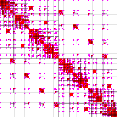
Figure 3: Visualisation of the storage costs of an $\mathcal{H}^{2}$-matrix.

The $\mathcal{H}^{2}$-matrix scheme scales linearly in the number of degrees of freedom [51].

Theorem 2 (Complexity estimates).

Let $\mathcal{T}(I\times J)$ be sparse in the sense that a constant $C_{sp}$ exists such that

$$\#\left\{c^{\prime}\in\mathcal{T}(J):r\times s^{\prime}\in\mathcal{T}(I\times J)\right\},\#\left\{r^{\prime}\in\mathcal{T}(I):r^{\prime}\times s\in\mathcal{T}(I\times J)\right\}\leq C_{sp}$$

for all $r\in\mathcal{T}(I)$ and $c\in\mathcal{T}(J)$. Then, the $\mathcal{H}^{2}$-matrix $\widetilde{G}$ requires

$$\mathcal{O}(p(\#I+\#J))$$

units of storage and the matrix-vector multiplication can be performed in just as many operations.

The number of interpolation points $p=m^{3}$ equals the rank of the low-rank factorisations in the far field and ultimately depends on the desired accuracy $\varepsilon>0$ of the approximation. We have

$$p=\mathcal{O}({-\log(\varepsilon)}^{4})$$

in general, cf. [52].

Remark 3.

Similar results hold for the kernel functions of the double layer and hyper-singular operator as well, see [50].

5 Adaptive Cross Approximation

Returning to the setting of (19), namely the approximation of the tensor

$$\boldsymbol{\mathcal{V}}[i,j,k]=V_{k}[i,j],$$

we have the preliminary result that each slice $V_{k}$ is given in form of an $\mathcal{H}^{2}$-matrix. Since the geometry $\Gamma$ is fixed for all times, we can construct a partition that does not depend on the particular frequency $s_{k}$. Therefore, we can select the same set of clusters $\mathcal{T}(I)$ and $\mathcal{T}(J)$ for all $V_{k}$. In this way, the partition $\mathcal{P}$ as well as the cluster bases ${\left(U_{r}\right)}_{r\in\mathcal{T}(I)}$ and ${\left(W_{c}\right)}_{c\in\mathcal{T}(J)}$ have to be built only once and are shared between all $V_{k}$. The latter only differ in the coupling matrices and near-field entries, which have to be computed separately for each frequency $s_{k}$.

Since all $V_{k}$ are partitioned identically, the tensor $\boldsymbol{\mathcal{V}}$ defined in (19) inherits their block structure in the sense that it can be decomposed according to $\mathcal{P}$ by simply ignoring the frequency index $k$.

Definition 6.

Let $K=\{0,\ldots,N-1\}$ and $\mathcal{T}(K)=\{K\}$. In the current context, we define $\boldsymbol{\mathcal{P}}\in\mathcal{T}(I\times J\times K)$ to be the tensor partition with blocks

$$b=r\times c\times K,\quad r\times c\in\mathcal{P},$$

which are admissible or inadmissible whenever $r\times c\in\mathcal{P}$ is admissible or inadmissible, respectively.

Naturally, this construction implies that the far-field blocks of $\boldsymbol{\mathcal{V}}$ are given in low-rank format,

$$\boldsymbol{\mathcal{V}}[r,c,k]=U_{r}\,S_{b,k}\,W_{c}^{H},\quad k=0,\ldots,N-1,$$

with $S_{b,k}$ being the coupling matrix of $b$ for the frequency $s_{k}$. If we collect the matrices $S_{b,k}$ in the tensor $\boldsymbol{\mathcal{S}}_{b}$ in the same manner as $V_{k}$ in $\boldsymbol{\mathcal{V}}$, we can factor out the cluster bases $U_{r}$ and $W_{c}$ using the tensor product from Definition 7,

$$\boldsymbol{\mathcal{V}}[r,c,K]=\boldsymbol{\mathcal{S}}_{b}\times_{1}U_{r}\times_{2}\overline{W_{c}}.$$

The coupling tensor $\boldsymbol{\mathcal{S}}_{b}$ consists of kernel evaluations of the transformed fundamental solution,

$$\boldsymbol{\mathcal{S}}_{b}[\mu,\nu,k]=\frac{e^{\textstyle{-s_{k}\left\lvert\xi_{c,\nu}-\xi_{r,\mu}\right\rvert}}}{4\pi\left\lvert\xi_{c,\nu}-\xi_{r,\mu}\right\rvert},$$

which is smooth in $B_{r}\times B_{c}$ but also in the frequency $s\in\mathbb{C}$. The latter holds true even for the near-field, whose entries are

$$\boldsymbol{\mathcal{V}}[i,j,k]=\int\limits_{\Gamma}\int\limits_{\Gamma}\frac{e^{\textstyle{-s_{k}\left\lvert y-x\right\rvert}}}{4\pi\left\lvert y-x\right\rvert}\varphi_{j}^{0}(y)\mathop{dS(y)}\varphi_{i}^{0}(x)\mathop{dS(x)}.$$

Hence, it is feasible to compress the tensor even further with respect to the frequency index $k$. In particular, the above discussion shows that we may proceed separately for each block $b\in\boldsymbol{\mathcal{P}}$, which represents either a dense block $\boldsymbol{\mathcal{V}}[b]$ in the near-field or a coupling block $\boldsymbol{\mathcal{S}}_{b}$ in the far-field.

5.1 Multivariate Adaptive Cross Approximation

Let $\boldsymbol{\mathcal{G}}\in\mathbb{C}^{m\times n\times p}$ be a tensor. The multivariate adaptive cross approximation (MACA) introduced in [53] finds a low-rank approximation of rank $r\leq p$ of the form

$$\boldsymbol{\mathcal{G}}\approx\boldsymbol{\mathcal{G}}^{(r)}=\sum_{\ell=1}^{r}C_{\ell}\times_{3}d_{\ell}$$ (25)

with matrices $C_{\ell}\in\mathbb{C}^{m\times n}$ and vectors $d_{\ell}\in\mathbb{C}^{p}$ as illustrated in Figure 4. The main idea is to reuse the original entries of the tensor.

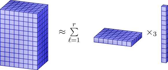
Figure 4: Visualisation of the low-rank factorisation.

Starting from $\boldsymbol{\mathcal{R}}^{(0)}=\boldsymbol{\mathcal{G}}$, we pick a non-zero pivot element in $\boldsymbol{\mathcal{R}}^{(\ell)}$ with index $(i_{\ell},j_{\ell},k_{\ell})$ and select the corresponding matrix slice and fibre for our next low-rank update, i.e.

$$C_{\ell}=\boldsymbol{\mathcal{R}}^{(\ell)}[1:m,1:n,k_{\ell}],\quad d_{\ell}={\boldsymbol{\mathcal{R}}^{(\ell)}[i_{\ell},j_{\ell},k_{\ell}]}^{-1}\boldsymbol{\mathcal{R}}^{(\ell)}[i_{\ell},j_{\ell},1:p].$$

Then, we compute the residual $\boldsymbol{\mathcal{R}}^{(\ell+1)}$ by subtracting their tensor product,

$$\boldsymbol{\mathcal{R}}^{(\ell+1)}=\boldsymbol{\mathcal{R}}^{(\ell)}-C_{\ell}\times_{3}d_{\ell}=\boldsymbol{\mathcal{R}}^{(\ell)}-\frac{\boldsymbol{\mathcal{R}}^{(\ell)}[1:m,1:n,k_{\ell}]\times_{3}\boldsymbol{\mathcal{R}}^{(\ell)}[i_{\ell},j_{\ell},1:p]}{\boldsymbol{\mathcal{R}}^{(\ell)}[i_{\ell},j_{\ell},k_{\ell}]}.$$

The residual $\boldsymbol{\mathcal{R}}^{(\ell+1)}=\boldsymbol{\mathcal{G}}-\boldsymbol{\mathcal{G}}^{(\ell)}$ measures the accuracy of the approximation. After $r=\ell$ steps we obtain the low-rank factorisation (25). By construction, the cross entries successively vanish, i.e.

$$\boldsymbol{\mathcal{R}}^{(r)}[i,j,k_{\ell}]=\boldsymbol{\mathcal{R}}^{(r)}[i_{\ell},j_{\ell},k]=0,\quad\ell=0,\ldots,r-1,$$

which implies $\boldsymbol{\mathcal{R}}^{(p+1)}=0$ and hence $r\leq p$. Figure 5 depicts one complete step of the MACA. We extract the cross consisting of $C_{\ell}$ and $d_{\ell}$ from $\boldsymbol{\mathcal{R}}^{(\ell)}$ and subtract the update $C_{\ell}\times_{3}d_{\ell}$, thereby eliminating the respective cross from $\boldsymbol{\mathcal{R}}^{(\ell+1)}$.

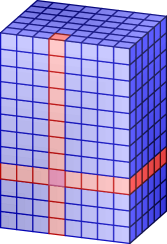
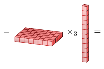
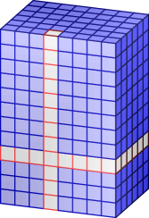
Figure 5: One step of the MACA.

The choice of the pivoting strategy is the crucial part of the algorithm. On the one hand, it should lead to nearly optimal results, in the sense that high accuracy is achieved with relatively low rank. On the other hand, it should be reliable and fast, otherwise it would become a bottleneck of the algorithm. Different pivoting strategies are available [30], but we restrict ourselves to finding the maximum entries in $C_{\ell}$ and $d_{\ell-1}$, i.e. we choose $(i_{\ell},j_{\ell},k_{\ell})$ such that

$$\left\lvert d_{\ell-1}[k_{\ell}]\right\rvert =\max_{k}\left\lvert d_{\ell-1}[k]\right\rvert,$$

$$\left\lvert C_{\ell}[i_{\ell},j_{\ell}]\right\rvert =\max_{i,j}\left\lvert C_{\ell}[i,j]\right\rvert,$$

with $k_{1}=0$. Throughout the algorithm, only $r$ slices and fibres of the original tensor $\boldsymbol{\mathcal{G}}$ are used. Thus, there is no need to build the whole tensor $\boldsymbol{\mathcal{G}}$ in order to approximate it and its entries are computed only on demand. This feature presents a clear advantage of the ACA, especially in BEM, where the generation of the entries is expensive. In this regard, the routine entry in Algorithm 2 is understood to be a call-back that computes the entries of $\boldsymbol{\mathcal{G}}$ at the time of its call. Moreover, the tensors $\boldsymbol{\mathcal{G}}^{(\ell)}$ are never formed explicitly but are stored in the low-rank format.

Algorithm 2 MACA

1:procedure maca(entry, $\displaystyle\varepsilon$)

2:     $\displaystyle\boldsymbol{\mathcal{G}}^{(0)}=0$, $\displaystyle k_{1}=0$ and $\displaystyle\ell=0$.

3:     do

4:         $\displaystyle\ell=\ell+1$

5:         $\displaystyle C_{\ell}[i,j]=\textsc{entry}(i,j,k_{\ell})-\boldsymbol{\mathcal{G}}^{(\ell-1)}[i,j,k_{\ell}],\quad i=1,\ldots,n,\ j=1,\ldots,m$

6:         $\displaystyle C_{\ell}[i_{\ell},j_{\ell}]=\max_{i,j}\left\lvert C_{\ell}[i,j]\right\rvert$

7:         if $\displaystyle C_{\ell}[i_{\ell},j_{\ell}]=0$ then

8:              $\displaystyle\ell=\ell-1$

9:              break

10:         end if

11:         $\displaystyle d_{\ell}[k]={C_{\ell}[i_{\ell},j_{\ell}]}^{-1}\left(\textsc{entry}(i_{\ell},j_{\ell},k)-\boldsymbol{\mathcal{G}}^{(\ell-1)}[i_{\ell},j_{\ell},k]\right),\quad k=1,\ldots,p$

12:         $\displaystyle\boldsymbol{\mathcal{G}}^{(\ell)}=\boldsymbol{\mathcal{G}}^{(\ell-1)}+C_{\ell}\times_{3}b_{\ell}$

13:         $\displaystyle k_{\ell+1}=\operatorname*{arg\,max}_{k}{\left\lvert d_{\ell}[k]\right\rvert}$

14:     while $\displaystyle\left\lVert C_{\ell}\right\rVert_{F}\left\lVert d_{\ell}\right\rVert_{2}>\varepsilon\left\lVert\boldsymbol{\mathcal{G}}^{(\ell)}\right\rVert_{F}$

15:     $\displaystyle r=\ell-1$

16:     return $\displaystyle\boldsymbol{\mathcal{G}}^{(r)}=\sum_{\ell=1}^{r}C_{\ell}\times_{3}d_{\ell}$

17:end procedure

Here, we terminate the algorithm if the low-rank update $C_{\ell}\times_{3}d_{\ell}=\boldsymbol{\mathcal{G}}_{\ell}-\boldsymbol{\mathcal{G}}_{\ell-1}$ is sufficiently small compared to $\boldsymbol{\mathcal{G}}^{(\ell)}$. Likewise, this stopping criterion does not require the expansion of $\boldsymbol{\mathcal{G}}^{(\ell)}$ due to the identity

$$\left\lVert\boldsymbol{\mathcal{G}}^{(\ell)}\right\rVert_{F}^{2} =\sum_{i,j,k}\left\lvert\sum_{\ell=1}^{r}C_{\ell}[i,j]b_{\ell}[k]\right\rvert^{2}$$

$$=\sum_{\ell,\ell^{\prime}=1}^{r}\left(\sum_{i,j}C_{\ell}[i,j]\,\overline{C_{\ell^{\prime}}[i,j]}\right)\left(\sum_{k}b_{\ell}[k]\,\overline{b_{\ell^{\prime}}[k]}\right).$$

Neglecting the numerical work needed to compute the entries of $\boldsymbol{\mathcal{G}}$, the overall complexity of the MACA amounts to $\mathcal{O}(r^{2}(nm+p))$.

If we collect the vectors $d_{\ell}$ in the matrix $D^{(r)}\in\mathbb{C}^{p\times r}$ and the matrices $C_{\ell}$ in the tensor $\boldsymbol{\mathcal{C}}^{(r)}\in\mathbb{C}^{m\times n\times r}$, we obtain the short representation

$$\boldsymbol{\mathcal{G}}^{(r)}=\boldsymbol{\mathcal{C}}^{(r)}\times_{3}D^{(r)},$$ (26)

which is equivalent to (25).

Remark 4.

A tensor $\boldsymbol{\mathcal{X}}\in\mathbb{C}^{I_{1}\times\cdots\times I_{d}}$ can be unfolded into a matrix by rearranging the index sets, which is called matricisation. For instance, the mode-$j$ unfolding $\mathcal{M}_{j}(\boldsymbol{\mathcal{X}})\in\mathbb{C}^{I_{j}\times(\Pi_{k\neq j}I_{k})}$ is defined by

$$\mathcal{M}_{j}(\boldsymbol{\mathcal{X}})[i_{j},(i_{1},\ldots,i_{j-1},i_{j+1},\ldots,i_{d})]=\boldsymbol{\mathcal{X}}[i_{1},\ldots,i_{d}].$$

With this in mind, it turns out that the MACA is in fact the standard ACA applied to a matricisation of the tensor. In our special case, it is the mode-3 unfolding.

Due to Remark 4, we can derive error bounds for the approximant $\boldsymbol{\mathcal{G}}^{(r)}$ based on standard results for the ACA.

Theorem 3 (Approximation error).

Let $\boldsymbol{\mathcal{G}}$ be either a dense block $\boldsymbol{\mathcal{V}}[b]$ or a coupling block $\boldsymbol{\mathcal{S}}_{b}$. Under the assumptions of [30, Theorem 3.35], there exist $0<\rho<1$ and $C>0$ such that the residual satisfies

$$\left\lVert\boldsymbol{\mathcal{R}}^{(\ell)}\right\rVert_{F}=\left\lVert\boldsymbol{\mathcal{G}}-\boldsymbol{\mathcal{G}}^{(\ell)}\right\rVert_{F}<C\rho^{\ell+1},\quad\ell=1,\ldots,N.$$

The constant $C>0$ depends on the block $b$ and on the distribution of the frequencies in the CQM (11).

Proof.

At first, we parameterise $s$ according to (11),

$$s(\theta)=\frac{\chi\left(R\cdot e^{\textstyle{\pi\imath\theta}}\right)}{\Delta t},\quad\theta\in[-1,1].$$

Then, the entries of $\boldsymbol{\mathcal{G}}$ are obtained by collocation of the functions

$$F_{ij}(\theta) =\int\limits_{\Gamma}\int\limits_{\Gamma}\frac{e^{\textstyle{{-s(\theta)\left\lvert y-x\right\rvert}}}}{4\pi\left\lvert y-x\right\rvert}\varphi_{j}^{0}(y)\mathop{dS(y)}\varphi_{i}^{0}(x)\mathop{dS(x)},$$

$$G_{\mu\nu}(\theta) =\frac{e^{\textstyle{-s(\theta)\left\lvert\xi_{c,\nu}-\xi_{r,\mu}\right\rvert}}}{4\pi\left\lvert\xi_{c,\nu}-\xi_{r,\mu}\right\rvert}$$

at $\theta=k/N$. Since they are analytic in $\theta$, we may use [54, Section 68 (76)] to bound the error of the best polynomial approximation of degree $\ell$,

$$\inf_{m\in\mathcal{P}_{\ell}}\left\lVert f-m\right\rVert_{\infty,[-1,1]}<\frac{2M}{1-\rho}\rho^{\ell+1},$$

where $f=F_{ij},G_{\mu\nu}$, $0<\rho<1$ and $M$ is chosen such that the absolute value of $f$ is less than $M$ within an ellipse in the complex plane whose foci are at $-1$ and $1$ and the sum of whose semi-axes is $1/\rho$. Hence, the application of [30, Theorem 3.35] yields the desired bound. ∎∎

Theorem 3 also justifies the choice of our stopping criterion. If we assume

$$\left\lVert\boldsymbol{\mathcal{R}}^{(\ell+1)}\right\rVert_{F}\leq\delta\left\lVert\boldsymbol{\mathcal{R}}^{(\ell)}\right\rVert_{F},$$

then we obtain

$$\left\lVert\boldsymbol{\mathcal{R}}^{(r)}\right\rVert_{F}\leq\delta\left\lVert\boldsymbol{\mathcal{G}}\right\rVert_{F}$$

by setting $\varepsilon=\delta(1-\delta)/(1+\delta)$.

6 Combined Algorithm

We are ready to state the complete algorithm, see Algorithm 3, for the low-rank approximation of the boundary element tensors from Section 3.2. In the first step, we build the cluster bases and construct a partition of the associated tensor (19) as outlined in Section 4 and Definition 6. In the second step, we apply the MACA from Section 5 to each block of the partition and obtain low-rank factorisations of the form (26). Eventually, we end up with a hierarchical tensor approximation, which reads

$$\boldsymbol{\mathcal{V}}[b] \approx\boldsymbol{\mathcal{C}}_{b}\times_{3}D_{b}, b\in\boldsymbol{\mathcal{P}}^{-},$$ (27)

$$\boldsymbol{\mathcal{V}}[b] \approx\boldsymbol{\mathcal{C}}_{b}\times_{1}U_{r}\times_{2}\overline{W_{c}}\times_{3}D_{b}, b\in\boldsymbol{\mathcal{P}}^{+}.$$

Besides the calls of the MACA routine, Algorithm 3 is identical to Algorithm 1.

Algorithm 3 Combined Algorithm

1:procedure main(${\left\{\psi_{i}\right\}}_{i\in I}$, ${\left\{\varphi_{j}\right\}}_{j\in J}$, ${\left\{s_{n}\right\}}_{n=1,\ldots,N}$, $n_{\min}$, $\eta$, $m$, $\varepsilon$)

2:     $\mathcal{T}(I)$ = cluster(${\left\{\psi_{i}\right\}}_{i\in I}$, $n_{\min}$),  $\mathcal{T}(J)$ = cluster(${\left\{\varphi_{j}\right\}}_{j\in J}$, $n_{\min}$)

3:     $rb$ = clusterbasis($I$, $m$), $cb$ = clusterbasis($J$, $m$)

4:     $\mathcal{P}$ = partition($\mathcal{T}(I)$, $\mathcal{T}(J)$, $\eta$)

5:     for $b\in\mathcal{P}$ do$\triangleright$ Call MACA for each block

6:         if $b$ is admissible then

7:              $\boldsymbol{\mathcal{C}}_{b}$, $B_{b}$ = maca(far, $b$, $\varepsilon$)

8:         else

9:              $\boldsymbol{\mathcal{C}}_{b}$, $B_{b}$ = maca(near, $b$, $\varepsilon$)

10:         end if

11:     end for

12:     return $\boldsymbol{\mathcal{A}}=\left\{{\left\{\boldsymbol{\mathcal{C}}_{b},B_{b}\right\}}_{b\in\mathcal{P}},rb,cb\right\}$

13:end procedure

14:

15:procedure far($\mu$, $\nu$, $n$)

16:     return $g(\xi_{r,\mu},\xi_{c,\nu},s_{n})$ $\triangleright$ Entries of coupling tensors

17:end procedure

18:

19:procedure near($i$, $j$, $n$)

20:     return $\int\limits_{\Gamma}\int\limits_{\Gamma}g(x,y,s_{n})\psi_{j}(y)\mathop{dS(y)}\varphi_{i}(x)\mathop{dS(x)}$ $\triangleright$ Entries of dense blocks

21:end procedure

6.1 Error analysis

Before we discuss computational advantages of this algorithm, we briefly state a basic result for the approximation error.

Corollary 1 (Tensor Approximation Error).

For every $\varepsilon\geq 0$, we find an approximation $\widetilde{\boldsymbol{\mathcal{V}}}$ of $\boldsymbol{\mathcal{V}}$ generated by Algorithm 3 which satisfies

$$\left\lVert\boldsymbol{\mathcal{V}}-\widetilde{\boldsymbol{\mathcal{V}}}\right\rVert_{F}\leq\varepsilon.$$

Proof.

For admissible blocks $b\in\boldsymbol{\mathcal{P}}^{+}$ we observe that the first term in

$$\left\lVert\boldsymbol{\mathcal{V}}[b]-\boldsymbol{\mathcal{C}}_{b}\times_{1}U_{r}\times_{2}\overline{W_{c}}\times_{3}D_{b}\right\rVert_{F} \leq\left\lVert\boldsymbol{\mathcal{V}}[b]-\boldsymbol{\mathcal{S}}_{b}\times_{1}U_{r}\times_{2}\overline{W_{c}}\right\rVert_{F}$$

$$\quad+\left\lVert\left(\boldsymbol{\mathcal{C}}_{b}\times_{3}D_{b}-\boldsymbol{\mathcal{S}}_{b}\right)\times_{1}U_{r}\times_{2}\overline{W_{c}}\right\rVert_{F},$$

is controlled by the $\mathcal{H}^{2}$-approximation and the second one by the MACA. By virtue of Theorems 1 and 3, we can prescribe accuracies $\delta_{b}>0$ on the approximation error for every far-field block. Similarly, we can bound the error block-wisely in the near-field by $\delta_{b}$. Hence, we obtain the desired bound by choosing $\delta_{b}$ such that

$$\left\lVert\boldsymbol{\mathcal{V}}-\widetilde{\boldsymbol{\mathcal{V}}}\right\rVert^{2}_{F}\leq\sum_{b\in\boldsymbol{\mathcal{P}}}\delta_{b}^{2}\leq\varepsilon^{2}$$

is satisfied. ∎∎

Remark 5.

The construction and analysis of low-rank approximations does not depend on the particular kernel function. Therefore, other boundary element matrices can be treated equivalently.

6.2 Complexity and Fast Arithmetics

For admissible blocks, the low-rank approximation is given in the so called Tucker format [55].

Definition 7 (Tucker format).

For a tensor $\boldsymbol{\mathcal{X}}\in\mathbb{C}^{I_{1}\times\cdots\times I_{d}}$ the Tucker format of tensor rank $(p_{1},\ldots,p_{d})$ consists of matrices $A^{(j)}\in\mathbb{C}^{p_{j}\times I_{j}}$, $j=1,\ldots,d$, and a core tensor $\boldsymbol{\mathcal{C}}\in\mathbb{C}^{p_{1}\times\cdots\times p_{d}}$ such that

$$\boldsymbol{\mathcal{X}}=\boldsymbol{\mathcal{C}}\times_{j=1}^{d}A^{(j)},$$

with the tensor product from Definition 1. In the following, we call

$$p=\max_{1\leq j\leq d}p_{j}$$

the maximum rank of the Tucker representation.

One of the main advantages of the approximation in the Tucker format is the reduction in storage costs. From (27), we see that the Tucker representation with maximum rank $p$ requires less than $\mathcal{O}(p^{3}+pN+p\,\#r+p\,\#c)$ units of storage compared with $\mathcal{O}(N\,\#r\,\#c)$ for the dense block tensor. In addition, we improve the complexity even for inadmissible blocks from $\mathcal{O}(N\,\#r\,\#c)$ to $\mathcal{O}(p\,\#r\,\#c\,+pN)$. From these considerations, we immediately deduce the following Corollary.

Corollary 2 (Storage Complexity).

Under the assumptions of Theorem 2, the hierarchical tensor decomposition needs about

$$\mathcal{O}(p^{2}(\#I+\#J)+pN)$$

units of storage.

In addition, the low-rank structure allows us to substantially accelerate important steps of the CQM. We recall that the computation of the integration weights $\widehat{V}_{n}$ in (16) comprises a matrix-valued discrete Fourier transform of the auxiliary matrices $V_{\ell}$. If we use representation (25) instead, we can factor out the frequency-independent information, i.e.

$$\widehat{V}_{n} =\frac{R^{-n}}{N}\sum_{\ell=0}^{N-1}e^{\tfrac{-2\pi\imath}{N}n\ell}\sum_{k=1}^{p}C_{k}\,d_{k}[\ell]$$ (28)

$$=\sum_{k=1}^{p}C_{k}\frac{R^{-n}}{N}\sum_{\ell=0}^{N-1}e^{\tfrac{-2\pi\imath}{N}n\ell}d_{k}[\ell],\quad n=0,\ldots,N.$$

Therefore, the transform has to be performed solely on the vectors $d_{k}$,

$$\hat{d}_{k}[n]=\frac{R^{-n}}{N}\sum_{\ell=0}^{N-1}e^{\tfrac{-2\pi\imath}{N}n\ell}d_{k}[\ell],$$

with the result that the tensor of integration weights $\widehat{\boldsymbol{\mathcal{V}}}$ inherits the hierarchical low-rank format of the original tensor $\boldsymbol{\mathcal{V}}$. In particular, the decomposition (27) still holds with $D_{b}$ replaced by $\widehat{D}_{b}$, whose columns are precisely the transformed vectors $\hat{d}_{k}$. Thereby, we reduce the number of required FFTs from $\#r\,\#c$ to $p$ per block. The other major improvement concerns the computation of the right-hand sides in (18). There, discrete convolutions of the form

$$f_{n}=\sum_{k=0}^{n}\widehat{V}_{n-k}\,\underline{q}_{k}$$

need to be evaluated in each step. Once again, we insert (25) and obtain

$$f_{n}=\sum_{k=0}^{n}\sum_{\ell=1}^{r}d_{\ell}[n-k]C_{\ell}\,\underline{q}_{k}=\sum_{\ell=1}^{p}C_{\ell}\left(\sum_{k=0}^{n}d_{\ell}[n-k]\,\underline{q}_{k}\right).$$ (29)

This representation requires in $\mathcal{O}(p)$ matrix-vector multiplications, which amounts to $\mathcal{O}(pN)$ matrix-vector multiplications in total. This is significantly less than the $\mathcal{O}(N^{2})$ operations needed by the conventional approach.

In combination with fast $\mathcal{H}^{2}$-matrix arithmetic [51], the algorithm scales nearly linearly in the number of degrees of freedom $M$ and time steps $N$. This is shown Table 1, where we compare the storage and operation counts of our fast algorithm with those of the traditional ones. Note that the numerical effort for computing the tensor entries is not stated explicitly but is reflected in the storage complexity. If efficient preconditioners are available, we may replace the direct solver by an iterative algorithm to eliminate the quadratic term $M^{2}$.

		Computational
Approximation	Storage	DFT	RHS	Solving
None	$M^{2}N$	$M^{2}N\log(N)$	$M^{2}N^{2}$	$M^{3}+M^{2}N$
$\mathcal{H}^{2}$	$pMN$	$pMN\log(N)$	$pMN^{2}$	$M^{2}+MN$
$\mathcal{H}^{2}$ + MACA	$p^{2}M+pN$	$pN\log(N)$	$p^{2}MN$	$M^{2}+MN$

Table 1: Comparison of storage and computational complexity.

Remark 6.

In [41], an alternative method for solving (17) is presented. There, the convolutional structure is avoided by transforming to and from the Fourier domain. This approach leads to $N$ independent systems which involve the auxiliary matrices $V_{k}$ only. Thus, we may apply our approximation scheme also in this case to speed up the assembly of the matrices and reduce the number of matrix-vector multiplications needed to solve the systems.

7 Numerical Examples

In this section, we present numerical examples which confirm our theoretical results and show the efficiency of our new algorithm. In all experiments, we set the parameter $\eta$ in the admissibility condition (20) to $2.0$ and choose $R=10^{-5/N}$ in the CQM. The core implementation is based on the H2Lib software . The machine in use consists of two Intel Xenon Gold 6154 CPUs operating at $3.00$ GHz with $376$ GB of RAM.

7.1 Tensor Approximation

The first set of examples concerns the performance and accuracy of the tensor approximation scheme.

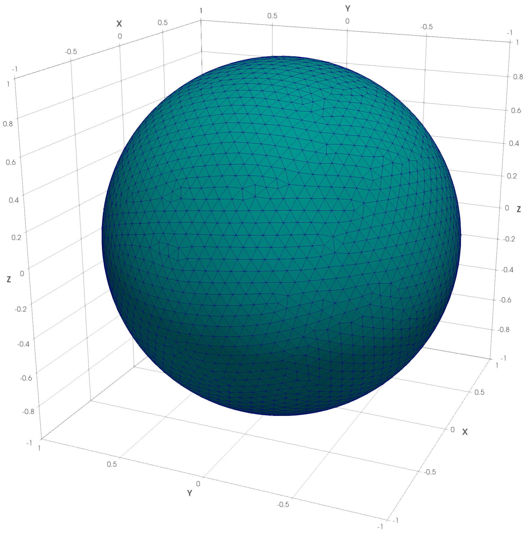
Figure 6: Spherical geometry $\Gamma$ used in the performance tests.

Let $\Gamma$ be the surface of a polyhedron $\Omega$, which approximates the sphere of radius $1$ with $M$ flat triangles, see Figure 6. We compare the dense tensor $\boldsymbol{\mathcal{V}}$ of single layer potentials with its low-rank factorisation $\widetilde{\boldsymbol{\mathcal{V}}}$ and study the impact of the interpolation order $m$ as well as accuracy $\varepsilon$ of the MACA on the approximation error, rank distribution, memory requirements and computation time.

We first set the number of degrees of freedom to $M=51200$ and time steps to $N=256$, resulting in a Courant number of $\Delta t/h\approx 0.83$. In Figure 8, the results for varying $\varepsilon$ and fixed $m=3,5,7$ are presented. Foremost, we observe that the relative error

$$e=\frac{\left\lVert\boldsymbol{\mathcal{V}}-\widetilde{\boldsymbol{\mathcal{V}}}\right\rVert_{F}}{\left\lVert\boldsymbol{\mathcal{V}}\right\rVert_{F}}.$$

in the Frobenius norm decreases with $\varepsilon$ until it becomes constant for high accuracies $\varepsilon\geq 10^{-4}$. This behaviour can be explained by Corollary 1. Even if the coupling blocks are reproduced exactly by the MACA, the $\mathcal{H}^{2}$-matrix approximation still dominates the total error. Moreover, the numerical results confirm that the maximal block-wise rank $r$ of the MACA depends logarithmically on $\varepsilon$ for fixed $m$. It stays below $30$ in contrast to $256$ time steps, which reveals the distinct low-rank character of the block tensors. Accordingly, our algorithm demands only for a small fraction of memory compared with the conventional dense approach. At worst, the compression rate reaches $3\%$ of the original storage requirements for $m=7$. For $m=3,5$ and optimal choice of $\varepsilon=10^{-2},10^{-3}$, we further improve it to $0.2\%$ and $0.8\%$, respectively. Similarly, the computation time needed for the assembly of the tensor is drastically reduced. For the optimal values of $\varepsilon$, the algorithm takes only a couple of seconds ($m=3,5$) or minutes ($m=7$) to compute the approximation of the single layer potentials. Furthermore, we report that both memory requirements and computation time scale logarithmically with $\varepsilon$.

To further demonstrate the benefits of the MACA, we consider the compression rate in comparison to the case when only $\mathcal{H}^{2}$-matrices are used. In Figure 8, the storage costs for the same test setup are presented. We notice that the inclusion of the MACA reduces the memory requirements to less than $15\%$, while the same level of accuracy is achieved.

If we modify the interpolation order $m$ instead, Theorems 1 and 2 indicate that the approximation error decreases exponentially while the storage costs rise polynomially. This is confirmed by the findings in Figure 9, where we set $\varepsilon=10^{-m}$ to ensure that MACA error is negligible. Indeed, we see that the error $e$ is roughly halved whenever $m$

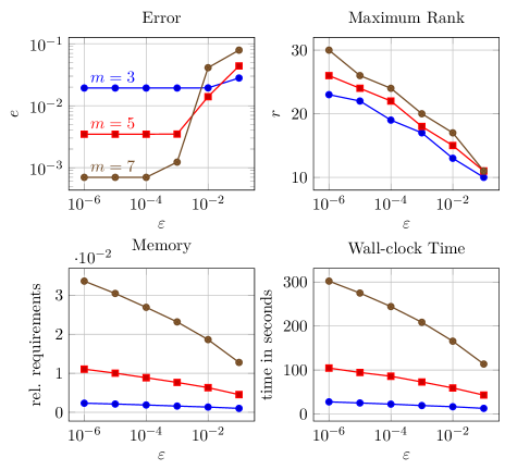
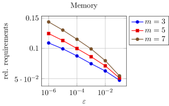
Figure 7: Results for $M=51200$, $N=256$, $m=3,5,7$ and improving accuracy $\varepsilon$ of the MACA.

Figure 8: Storage requirements relative to the plain $\mathcal{H}^{2}$-matrix approach for $M=51200$, $N=256$, $m=3,5,7$ and varying $\varepsilon$.

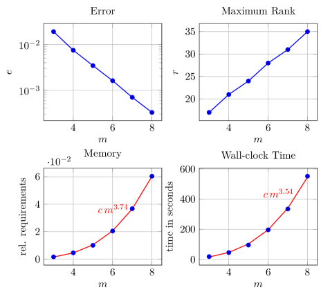
Figure 9: Results for $M=51200$, $N=256$, $\varepsilon=10^{-m}$ and increasing interpolation order $m$.

is increased by one and reaches almost $10^{-4}$ for $m=8$. The upper right plot shows that the simultaneous change in $\varepsilon$ and $m$ leads to a linear growth of the MACA rank $r$ in terms of $m$. Since the storage and computational complexity for fixed $M$ and $N$ is of order $\mathcal{O}(p\,r)$, where $p=m^{3}$ is the interpolation rank, we observe that the memory and time consumption scale approximately as $\mathcal{O}(m^{4})$. Note that in contrast to the prior example, the partition changes for every $m$, since the latter directly affects the clustering. We conclude that the algorithm yields accurate approximations with high compression rates in short amounts of time. Moreover, we have seen that the performance is more sensitive to a change in interpolation order $m$ than in the MACA parameter $\varepsilon$. Hence, we recommend to select $\varepsilon$ on the basis of $m$ and not the other way around.

In the next two tests, we investigate the scaling of the algorithm in the number of degrees of freedom $M$ and time steps $N$. First off, we fix the Courant number $\Delta t/h=0.7$ and refine the mesh $\Gamma$ successively. The parameters $m=7$ and $\varepsilon=10^{-8}$ are chosen in such a way that the error $e$ is of the magnitude $10^{-3}$. Note that the approximation is more accurate for small $M$ as the near-field still occupies a large part of the partition. The results are depicted in Figure 11, where the number of time steps is added for the sake of completeness. First of all, we notice that the storage and computational complexity are linear in $M$ in accordance with Corollary 2. Although the maximal rank $r$ grows logarithmically at the same time, it does not influence the overall performance. This is probably due to the average rank staying almost constant in comparison. The rank distribution is visualised in form of a heat map in Figure 11.

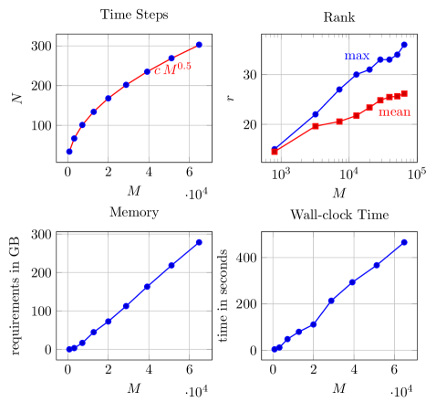
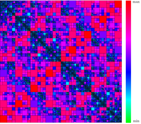
Figure 10: Results for constant courant number $\Delta t/h=0.7$, $m=7$, $\varepsilon=10^{-8}$ and increasing number of degrees of freedom $M$.

Figure 11: Exemplary rank distribution of the tensor partition for $M=51200$ degrees of freedom and $N=768$ time steps.

The dependence on the number of time steps $N$ for constant $M=51200$ is illustrated in Figure 12. We use the same values for the parameters as before, i.e., $m=7$ and $\varepsilon=10^{-8}$, and now change the Courant number $\Delta t/h$ instead of $M$. The rise of the error $e$ is attributed to the change in frequencies $s_{\ell}$. Since they grow in modulus, the interpolation quality worsens with increasing $N$. We summarise that the approximation scheme has linear complexity in both the number of degrees of freedom $M$ and time steps $N$ for fixed tolerance $\varepsilon$ and interpolation order $m$.

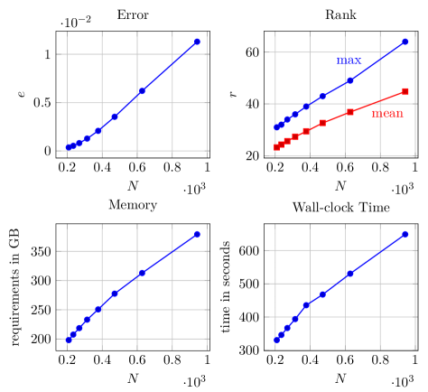
Figure 12: Results for $M=51200$, $m=7$, $\varepsilon=10^{-8}$ and increasing number of time steps $N$.

7.2 Scattering Problem

In this last section, we perform benchmarks for our fast CQM algorithm from Section 6 and study the effect of the tensor approximation on the solution of the wave problem.

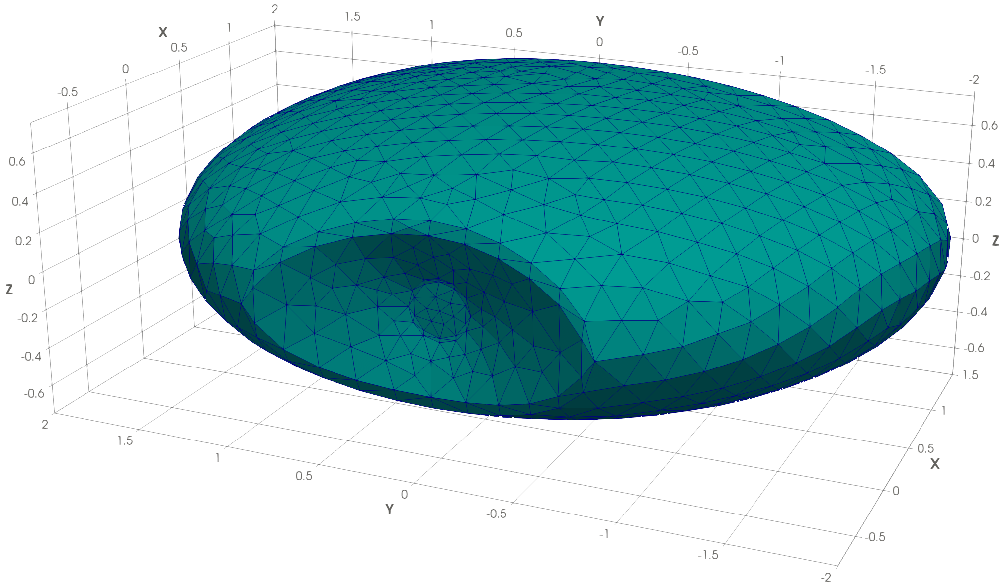
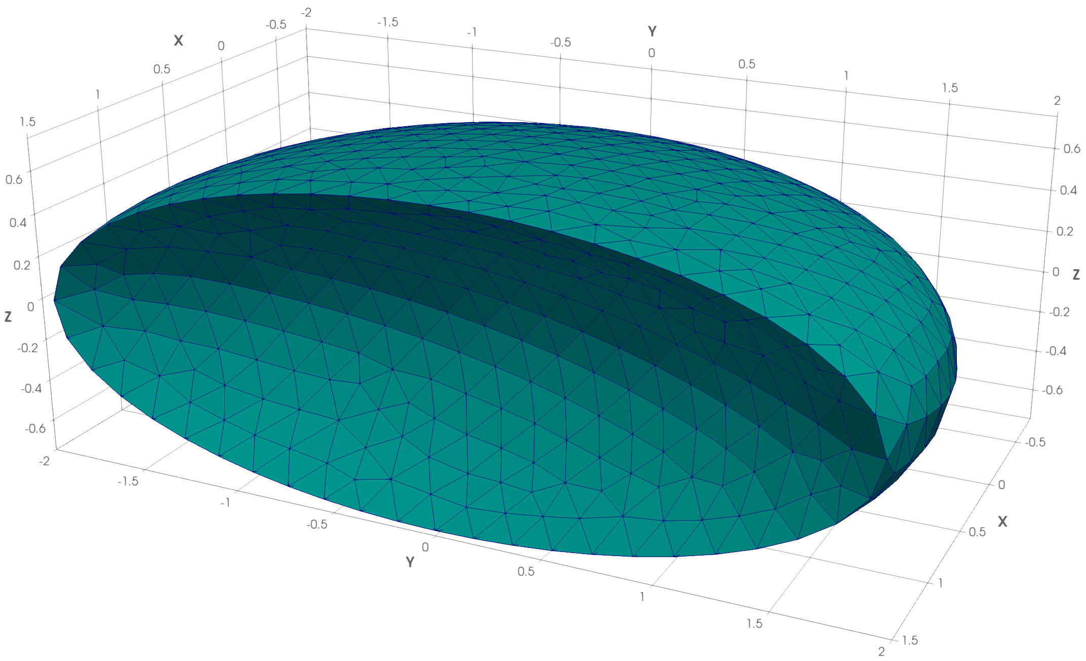
Figure 13: Front view and back view of the obstacle.

To that end, we switch settings to the model problem (1) posed in the exterior of the geometry pictured in Figure 13. The spherical wave

$$u(x,t)=\frac{f(t-\left\lvert x\right\rvert)}{\left\lvert x\right\rvert},\quad f(z)=\left\{\begin{aligned} &\cos(5z+1)-1,&&z>-1/5,\\ &\,0,&&z\leq-1/5,\end{aligned}\right.$$

serves as the exact solution. We shift the time variable such that $u$ reaches the boundary $\Gamma$ right after $t=0$.

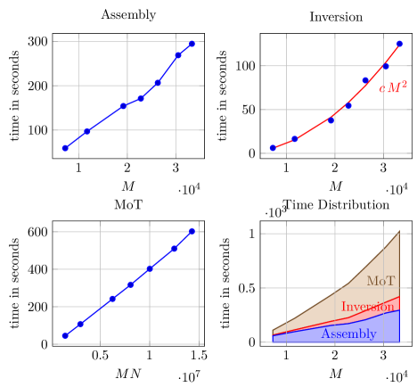
Figure 14: Results for constant courant number $\Delta t/h=0.2$, $m=5$, $\varepsilon=10^{-4}$ and increasing number of degrees of freedom $M$.

The first part of tests concerns the fast arithmetics developed in Section 6.2. To simplify matters, we impose pure Dirichlet conditions on $\Gamma_{D}=\Gamma$ and solve for the Neumann trace $q_{n}$ in

$$\widehat{V}_{0}\underline{q}_{n}=\left(-\frac{1}{2}I+\widehat{K}_{0}\right)\underline{g}^{D}_{n}+\sum_{k=0}^{n-1}\left(\widehat{K}_{n-k}\underline{g}^{D}_{k}-\widehat{V}_{n-k}\underline{q}_{k}\right),\quad n=0,\ldots,N,$$ (30)

as outlined in Section 3.2. We choose $T=4.7$ as the final time. We identify three major stages of the algorithm, firstly the assembly of the tensors, secondly the inversion of $\widehat{V}_{0}$ and thirdly the step-by-step solution of the linear systems, which is also known as marching-in-on-time (MoT). In Figure 14, we visualise how the running time is distributed among the stages and how they scale in $N$ and $M$ for fixed parameters $m=5$ and $\varepsilon=10^{-4}$. Overall, we see that the numerical results are consistent with the estimates from Table 1. Beginning with the tensor assembly, we once again observe linear complexity in $M$. The assembly comprises the fast transformation from (28) and is not explicitly listed, since it requires less than $2$ seconds to perform in all cases. The LU decomposition of the matrix $\widehat{V}_{0}$ involves $\mathcal{O}(M^{2})$ operations but it nevertheless poses the least demanding part of the algorithm for our problem size. On the other hand, the iterative solution of (30) takes the largest amount of time. However, the application of (29) allows for the fast computation of the right-hand sides in just $\mathcal{O}(MN)$. This presents a significant speed up over the conventional implementation. Taking into account that $N\sim M^{1/2}$ for a constant Courant number, we expect the second stage to be the most expensive for very large $M$. Therefore, it might be advantageous to switch to iterative algorithms to solve the linear systems if efficient preconditioners are available.

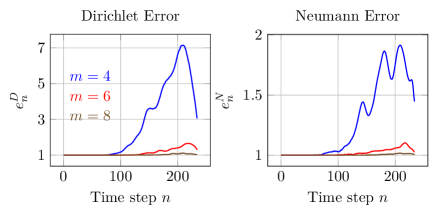
Figure 15: Results for constant $M=19182$, $N=235$, $\varepsilon=10^{-8}$ and increasing interpolation order $m$.

For the last example, we split the boundary $\Gamma$ in Neumann and Dirichlet parts $\Gamma_{N}$ and $\Gamma_{D}$ and replace the Dirichlet conditions by mixed conditions. The Neumann boundary $\Gamma_{N}$ covers the upper half of $\Gamma$ with positive component $x_{3}>0$, while the rest of $\Gamma$ accounts to the Dirichlet part. Furthermore, we consider the time interval $(0,1.7)$. We denote by $u_{n}$ and $q_{n}$ the exact solutions and compare them with the approximations $\tilde{u}_{n}$ and $\tilde{q}_{n}$ obtained by our fast CQM. We also include the reference solutions $\tilde{u}^{\textup{ref}}_{n}$ and $\tilde{q}^{\textup{ref}}_{n}$ provided by the dense version. In particular, we are interested in how the interpolation order $m$ affects the quality of the approximations, which we estimate by computing the deviations

$$e^{D}_{n}=\frac{\left\lVert u_{n}-\tilde{u}_{n}\right\rVert_{L^{2}(\Gamma)}}{\left\lVert u_{n}-\tilde{u}^{\textup{ref}}_{n}\right\rVert_{L^{2}(\Gamma)}},\quad e^{N}_{n}=\frac{\left\lVert q_{n}-\tilde{q}_{n}\right\rVert_{L^{2}(\Gamma)}}{\left\lVert q_{n}-\tilde{q}^{\textup{ref}}_{n}\right\rVert_{L^{2}(\Gamma)}},\quad n=0,\ldots,N,$$

A value close to one indicates that the interpolation error does not spoil the overall accuracy of the algorithm. We select a mesh with $M=19182$ triangles and set the number of time steps to $N=235$. The choice of $\varepsilon=10^{-8}$ guarantees that the MACA does not deteriorate the interpolation quality. The results for varying $m$ are depicted in Figure 15. We observe that the approximations show the same level of accuracy for $n\leq 75$ regardless of the interpolation order. Then, the interpolation error becomes noticeable for $m=4$ as $e^{D}_{n}$ and $e^{N}_{n}$ grow with $n$. The deviations from the reference solution are considerably smaller for $m=6$ and our approximation scheme has almost no impact on the accuracy for $m\geq 8$.

8 Conclusion

In this paper, we have presented a novel fast approximation technique for the numerical solution of wave problems by the CQM and BEM. We have given insights into the theoretical and practical aspects of our algorithm and have explained how it acts as a kind of hierarchical tensor approximation. Moreover, we have proposed fast arithmetics for the evaluations of the discrete convolutions in the CQM. In this way, we manage to reduce the complexity in terms of the number of spatial degrees of freedom $M$ and number of time steps $N$: the storage costs from $\mathcal{O}(M^{2}N)$ to $\mathcal{O}(M+N)$ and the computational costs from $\mathcal{O}(M^{2}N^{2}+M^{3})$ to $\mathcal{O}(MN+M^{2})$, where the quadratic factor can be dropped if efficient preconditioners are available. Therefore, we consider our work to be a step towards making large scale space-time simulations possible with BEM.

References

- [1] A. Bamberger and T. Ha Duong “Formulation variationnelle espace-temps pour le calcul par potentiel retardé de la diffraction d’une onde acoustique. I” In Math. Methods Appl. Sci. 8.3, 1986, pp. 405–435
- [2] F.-J. Sayas “Retarded potentials and time domain boundary integral equations” 50, Springer Series in Computational Mathematics Springer, Cham, 2016, pp. xv+242
- [3] M. E. Hassell, T. Qiu, T. Sánchez-Vizuet and F.-J. Sayas “A new and improved analysis of the time domain boundary integral operators for the acoustic wave equation” In J. Integral Equ. Appl. 29.1, 2017, pp. 107–136
- [4] M. Costabel and F.-J. Sayas “Time-Dependent Problems with the Boundary Integral Equation Method” In Encyclopedia of Computational Mechanics Second Edition John Wiley & Sons, Inc., New York-London-Sydney, 2017, pp. 1–24
- [5] P. Joly and J. Rodríguez “Mathematical aspects of variational boundary integral equations for time dependent wave propagation” In J. Integral Equations Appl. 29.1, 2017, pp. 137–187
- [6] W.J. Mansur “A Time-Stepping Technique to Solve Wave Propagation Problems using the Boundary Element Method”, 1983
- [7] P.W. Partridge, C.A. Brebbia and L. C. Wrobel “The dual reciprocity boundary element method”, International Series on Computational Engineering Springer, Dordrecht, 1991, pp. xvi+284
- [8] U. Langer and O. Steinbach “Space-Time Methods” Berlin, Boston: De Gruyter, 2019
- [9] H. Gimperlein, M. Maischak and E.P. Stephan “Adaptive time domain boundary element methods with engineering applications” In J. Integral Equations Appl. 29.1, 2017, pp. 75–105
- [10] H. Gimperlein, C. Özdemir, D. Stark and E.P. Stephan “hp-version time domain boundary elements for the wave equation on quasi-uniform meshes” In Comput. Methods Appl. Mech. Engrg. 356, 2019, pp. 145–174
- [11] D. Pölz, M. H. Gfrerer and M. Schanz “Wave propagation in elastic trusses: an approach via retarded potentials” In Wave Motion 87, 2019, pp. 37–57
- [12] D. Pölz and M. Schanz “Space-time discretized retarded potential boundary integral operators: quadrature for collocation methods” In SIAM J. Sci. Comput. 41.6, 2019, pp. A3860–A3886
- [13] C. Lubich “Convolution quadrature and discretized operational calculus. I” In Numer. Math. 52.2, 1988, pp. 129–145
- [14] C. Lubich “Convolution quadrature and discretized operational calculus. II” In Numer. Math. 52.4, 1988, pp. 413–425
- [15] C. Lubich “On the multistep time discretization of linear initial-boundary value problems and their boundary integral equations” In Numer. Math. 67.3, 1994, pp. 365–389
- [16] L. Banjai, C. Lubich and J. M. Melenk “Runge-Kutta convolution quadrature for operators arising in wave propagation” In Numer. Math. 119.1, 2011, pp. 1–20
- [17] L. Banjai, M. Messner and M. Schanz “Runge-Kutta convolution quadrature for the boundary element method” In Comput. Methods Appl. Mech. Engrg. 245/246, 2012, pp. 90–101
- [18] W. McLean “Strongly elliptic systems and boundary integral equations” Cambridge University Press, Cambridge, 2000, pp. xiv+357
- [19] M. Schanz and H. Antes “A new visco- and elastodynamic time domain: boundary element formulation” In Comput. Mech. 20.5, 1997, pp. 452–459
- [20] M. Hassell and F.-J. Sayas “Convolution quadrature for wave simulations” In Numerical Simulation in Physics and Engineering 9, SEMA SIMAI Springer Ser. Springer, Cham, 2016, pp. 71–159
- [21] M. Lopez-Fernandez and S. Sauter “Generalized convolution quadrature based on Runge-Kutta methods” In Numer. Math. 133.4, 2016, pp. 743–779
- [22] S. A. Sauter and M. Schanz “Convolution quadrature for the wave equation with impedance boundary conditions” In J. Comput. Phys. 334, 2017, pp. 442–459
- [23] L. Banjai and A. Rieder “Convolution quadrature for the wave equation with a nonlinear impedance boundary condition” In Math. Comp. 87.312, 2018, pp. 1783–1819
- [24] M. E. Hassell and F.-J. Sayas “A fully discrete BEM-FEM scheme for transient acoustic waves” In Comput. Methods Appl. Mech. Engrg. 309, 2016, pp. 106–130
- [25] J. Ballani, L. Banjai, S. Sauter and A. Veit “Numerical solution of exterior Maxwell problems by Galerkin BEM and Runge-Kutta convolution quadrature” In Numer. Math. 123.4, 2013, pp. 643–670
- [26] L. Kielhorn and M. Schanz “Convolution quadrature method-based symmetric Galerkin boundary element method for 3-d elastodynamics” In Internat. J. Numer. Methods Engrg. 76.11, 2008, pp. 1724–1746
- [27] M. Schanz “Wave Propagation in Viscoelastic and Poroelastic Continua: A Boundary Element Approach” 2, Lecture Notes in Applied and Computational Mechanics Springer, Berlin-Heidelberg, 2001
- [28] G. C. Hsiao, T. Sánchez-Vizuet, F.-J. Sayas and R. J. Weinacht “A time-dependent wave-thermoelastic solid interaction” In IMA J. Numer. Anal. 39.2, 2019, pp. 924–956
- [29] J. M. Melenk and A. Rieder “Runge-Kutta convolution quadrature and FEM-BEM coupling for the time-dependent linear Schrödinger equation” In J. Integral Equ. Appl. 29.1, 2017, pp. 189–250
- [30] M. Bebendorf “Hierarchical matrices” 63, Lecture Notes in Computational Science and Engineering Springer, Berlin, 2008, pp. xvi+290
- [31] S. Rjasanow and O. Steinbach “The fast solution of boundary integral equations”, Mathematical and Analytical Techniques with Applications to Engineering Springer, New York, 2007, pp. xii+279
- [32] W. Hackbusch “Hierarchical matrices: algorithms and analysis” 49, Springer Series in Computational Mathematics Springer, Heidelberg, 2015, pp. xxv+511
- [33] S. Börm, M. Löhndorf and J. M. Melenk “Approximation of integral operators by variable-order interpolation” In Numer. Math. 99.4, 2005, pp. 605–643
- [34] W. Hackbusch and S. Börm “Data-sparse approximation by adaptive -matrices” In Computing 69.1, 2002, pp. 1–35
- [35] M. Bebendorf “Approximation of boundary element matrices” In Numer. Math. 86.4, 2000, pp. 565–589
- [36] M. Bebendorf and S. Rjasanow “Adaptive low-rank approximation of collocation matrices” In Computing 70.1, 2003, pp. 1–24
- [37] W. Kress and S. Sauter “Numerical treatment of retarded boundary integral equations by sparse panel clustering” In IMA J. Numer. Anal. 28.1, 2008, pp. 162–185
- [38] W. Hackbusch, W. Kress and S. A. Sauter “Sparse convolution quadrature for time domain boundary integral formulations of the wave equation” In IMA J. Numer. Anal. 29.1, 2009, pp. 158–179
- [39] L Banjai and M. Kachanovska “Sparsity of Runge-Kutta convolution weights for the three-dimensional wave equation” In BIT 54.4, 2014, pp. 901–936
- [40] L. Banjai and M. Kachanovska “Fast convolution quadrature for the wave equation in three dimensions” In J. Comput. Phys. 279, 2014, pp. 103–126
- [41] L. Banjai and S. Sauter “Rapid solution of the wave equation in unbounded domains” In SIAM J. Numer. Anal. 47.1, 2009, pp. 227–249
- [42] A. M. Haider and M. Schanz “Generalization of adaptive cross approximation for time-domain boundary element methods” In PAMM 19.1, 2019, pp. e201900072
- [43] J.-L. Lions and E. Magenes “Non-homogeneous boundary value problems and applications. Vol. I–III” Springer, New York-Heidelberg, 1972–1973
- [44] I. Lasiecka, J.-L. Lions and R. Triggiani “Nonhomogeneous boundary value problems for second order hyperbolic operators” In J. Math. Pures Appl. (9) 65.2, 1986, pp. 149–192
- [45] D. Tataru “On the regularity of boundary traces for the wave equation” In Ann. Scuola Norm. Sup. Pisa Cl. Sci. (4) 26.1, 1998, pp. 185–206
- [46] I. Lasiecka and R. Triggiani “Sharp regularity theory for second order hyperbolic equations of Neumann type. I. nonhomogeneous data” In Ann. Mat. Pura Appl. (4) 157, 1990, pp. 285–367
- [47] J. Jackson “Classical electrodynamics” John Wiley & Sons, Inc., New York-London-Sydney, 1998, pp. xxi+808
- [48] E. Hairer, S. P. Nørsett and G. Wanner “Solving ordinary differential equations. I” 8, Springer Series in Computational Mathematics Springer, Berlin, 1993, pp. xvi+528
- [49] J. C. Nédélec “Acoustic and electromagnetic equations” 144, Applied Mathematical Sciences Springer, New York, 2001, pp. x+316
- [50] S. Börm “Efficient numerical methods for non-local operators” 14, EMS Tracts in Mathematics European Mathematical Society, Zürich, 2010, pp. x+432
- [51] S. Börm “-matrix arithmetics in linear complexity” In Computing 77.1, 2006, pp. 1–28
- [52] M. Bebendorf and W. Hackbusch “Existence of -matrix approximants to the inverse FE-matrix of elliptic operators with -coefficients” In Numer. Math. 95.1, 2003, pp. 1–28
- [53] M. Bebendorf “Adaptive cross approximation of multivariate functions” In Constr. Approx. 34.2, 2011, pp. 149–179
- [54] S. N. Bernšteĭn “Sobranie sočinenii. Tom I. Konstruktivnaya teoriya funkciĭ [1905–1930]” Izdat. Akad. Nauk SSSR, Moscow, 1952, pp. 581 pp. (1 plate)
- [55] W. Hackbusch “Tensor spaces and numerical tensor calculus” 42, Springer Series in Computational Mathematics Springer, Heidelberg, 2012, pp. xxiv+500