Atacama Compact Array Observations of the Pulsar-Wind Nebula of SNR 0540-69.3

Abstract

We present observations of the pulsar-wind nebula (PWN) region of SNR 0540-69.3. The observations were made with the Atacama Compact Array (ACA) in Bands 4 and 6. We also add radio observations from the Australia Compact Array (ATCA) at 3 cm. For $1.449-233.50$ GHz we obtain a synchrotron spectrum $F_{\nu}\propto\nu^{-\alpha_{\nu}}$, with the spectral index $\alpha_{\nu}=0.17\pm{0.02}$. To conclude how this joins the synchrotron spectrum at higher frequencies we include hitherto unpublished AKARI mid-infrared data, and evaluate published data in the ultraviolet (UV), optical and infrared (IR). In particular, some broad-band filter data in the optical must be discarded from our analysis due to contamination by spectral line emission. For the UV/IR part of the synchrotron spectrum, we arrive at $\alpha_{\nu}=0.87^{+0.08}_{-0.10}$. There is room for $2.5\times 10^{-3}~{}{\rm M}_{\odot}$ of dust with temperature $\sim 55$ K if there are dual breaks in the synchrotron spectrum, one around $\sim 9\times 10^{10}$ Hz, and another at $\sim 2\times 10^{13}$ Hz. The spectral index then changes at $\sim 9\times 10^{10}$ Hz from $\alpha_{\nu}=0.14\pm 0.07$ in the radio, to $\alpha_{\nu}=0.35^{-0.07}_{+0.05}$ in the millimetre to far-IR range. The ACA Band 6 data marginally resolves the PWN. In particular, the strong emission $\sim 1\hbox{$.\!\!^{\prime\prime}$}5$ south-west of the pulsar, seen at other wavelengths, and resolved in the 3-cm data with its 0$.\!\!^{\prime\prime}$8 spatial resolution, is also strong in the millimeter range. The ACA data clearly reveal the supernova remnant shell $\sim 20-35\arcsec$ west of the pulsar, and for the shell we derive $\alpha_{\nu}=0.64\pm{0.05}$ for the range $8.6-145$ GHz.

1 Introduction

The oxygen-rich ejecta of the $\sim 10^{3}$ year old LMC supernova remnant (SNR) 0540-69.3 (in short SNR0540) (Kirshner et al., 1989; Serafimovich et al., 2005) is evidence that SNR0540 is the result of an explosion of a massive, $\sim 20~{}{\rm M}_{\odot}$ (at zero-age main-sequence), progenitor (Chevalier, 2006; Williams et al., 2008; Lundqvist et al., 2011). The radiation emitted from the remnant manifests itself mainly through radio and X-ray emission from a shell of radius $\sim 20\arcsec-35\arcsec$, corresponding to $\sim 4.9-8.5$ pc at the 50 kpc distance of LMC (Manchester et al., 1993b; Gotthelf & Wang, 2000). Most of this emission comes from the western part of the shell.

The remnant contains the pulsar PSR B0540-69.3 (henceforth PSR0540), discovered as a pulsed ($P=50.2$ ms) X-ray source by Seward et al. (1984). Pulsations have subsequently also been detected in the optical (Middleditch & Pennypacker, 1985), at radio wavelengths (Manchester et al., 1993a), and recently in the UV (Mignani et al., 2019). The properties of PSR0540 are very similar to those of the Crab pulsar: it spins rapidly and it is young (spin down age 1660 yr).

Like the Crab pulsar, PSR0540 powers a pulsar-wind nebula (PWN), which we will refer to as PWN0540. The full size of PWN0540 in radio is $\sim 7\arcsec-8\arcsec$ across, with an inner core of $\sim 5\arcsec$ in diameter, also seen in the UV/optical (Caraveo et al., 1992; Serafimovich et al., 2004) radio (e.g., Manchester et al., 1993b) and X-rays (Gotthelf & Wang, 2000). The PWN emits synchrotron emission with a flux $F_{\nu}\propto\nu^{-\alpha_{\nu}}$, where $\alpha_{\nu}$ runs from $\sim 0.15$ in the radio (Brantseg et al., 2014) to a larger value in the optical (Serafimovich et al., 2004; Mignani et al., 2012).

PWN0540 is in no sense different from other PWNe when it comes to the shallow slope in radio; the vast majority of 39 PWNe studied in the radio have $\alpha_{\nu}\!\!\!\phantom{\leq}\smash{\buildrel\over{\lower 2.67502pt\hbox{$\buildrel\lower 2.14001pt\hbox{$\displaystyle<$}\over{\sim}$}}}\,\,0.3$ (Reynolds et al., 2017). Neither is the steepening towards higher photon energies unique. For example, the Crab PWN has a spectral break around $\sim 3\times 10^{10}$ Hz, where the spectral index changes from $\alpha_{\nu}\approx 0.3$ in the radio to $\alpha_{\nu}\approx 0.42$ at higher frequencies (Gomez et al., 2012). Such spectral breaks have also been seen in other PWNe (cf. Reynolds et al., 2017, and references therein).

The shape of the synchrotron radio/IR spectrum provides important information about the energy distribution of relativistic electrons and their radiative losses, and inhomogeneities within the PWN (Reynolds et al., 2017). For a power-law distribution for the energy of relativistic electrons, $dN/dE=N_{0}E^{-p}$, where $E=\gamma m_{e}c^{2}$ is the energy of the electrons and $\gamma$ is the Lorentz factor, the intensity of optically thin synchrotron emission is $\propto\nu^{-\alpha}$, where $\alpha=(p-1)/2$. A flat spectrum with $\alpha\sim 0.15$, as for PWN0540 in the radio, would then indicate $p\sim 1.3$. This is much shallower than $p\!\!\!\phantom{\geq}\smash{\buildrel\over{\lower 2.67502pt\hbox{$\buildrel\lower 2.14001pt\hbox{$\displaystyle>$}\over{\sim}$}}}\,\,2$ expected at shock fronts of relativistic shocks (e.g., Bykov et al., 2012), corresponding to $\alpha\!\!\!\phantom{\geq}\smash{\buildrel\over{\lower 2.67502pt\hbox{$\buildrel\lower 2.14001pt\hbox{$\displaystyle>$}\over{\sim}$}}}\,\,0.5$. Bucciantini et al. (2011) showed that a broken power-law energy distribution of the relativistic electrons can explain the shallow radio spectrum of the Crab PWN and a few other PWNe, and argued for that the relativistic electrons at the lowest energies could be accelerated in a turbulence zone in connection with the termination shock rather than via Fermi acceleration. In the work of Bucciantini et al. (2011), as well of others (e.g., Gelfand et al., 2009; Martin et al., 2012), particles are continuously injected into the PWN, with the energy spectrum of the injected particles being discontinuous or having a break.

There are models invoking reconnection as the source of particle acceleration (e.g., Clausen-Brown & Lyutikov, 2012; Cerutti et al., 2012; Sironi & Spitkovsky, 2011; Porth et al., 2016), and Lyutikov et al. (2019) argue that both Fermi-I and reconnection processes occur in the Crab PWN, and that this can explain the multiple spectral breaks for that PWN. Several spectral breaks are also evident in compiled IR-optical-X-ray spectra of the torus-like parts of other well-studied PWNe (PWN0540, 3C 58, J1124-5916 and G21.5-0.9, Zharikov et al., 2013), implying that multiple populations of relativistic particles are responsible for the emission in different spectral domains. In particular, the overall radio-to-X-ray spectrum of PWN0540 has been discussed by Serafimovich et al. (2004), Mignani et al. (2012), Lundqvist et al. (2011) and Brantseg et al. (2014), and it shows that the X-ray emission is stronger than expected from a power-law extrapolation of the IR/optical/UV spectrum. This indeed indicates the existence of more than one emission component. In addition, spatially resolved X-ray spectra of PWN0540 show that the steepness of the X-ray spectrum increases away from the torus region (Lundqvist et al., 2011), which is expected if the particles injected there experience adiabatic and synchrotron losses as they move away from that region. Such spatial variations tend to smooth spectral breaks in spatially integrated spectra of PWNe (e.g., Reynolds et al., 2017).

An established synchrotron contribution in the millimetre/IR range is needed to estimate possible additional continuum emission from supernova-produced dust. Prime examples of the latter in SNRs are the Crab Nebula (Gomez et al., 2012; Owen & Barlow, 2015), PWN G54.1+0.3 (Temim et al., 2017; Rho et al., 2018), Cas A (De Looze et al., 2017), and the young ($\!\!\!\phantom{\leq}\smash{\buildrel\over{\lower 2.67502pt\hbox{$\buildrel\lower 2.14001pt\hbox{$\displaystyle<$}\over{\sim}$}}}\,\,2.5$ kyr) remnants G11.2-0.3, G21.5-0.9 and G29.7-0.3 (Chawner et al., 2019). The most obvious case outside the Milky Way is SN 1987A (Matsuura et al., 2011, 2015; Indebetouw et al., 2014; Dwek & Arendt, 2015), which, like the SNRs mentioned, has substantial amounts of dust ($\!\!\!\phantom{\geq}\smash{\buildrel\over{\lower 2.67502pt\hbox{$\buildrel\lower 2.14001pt\hbox{$\displaystyle>$}\over{\sim}$}}}\,\,0.2~{}{\rm M}_{\odot}$) embedded within it.

Spitzer observations indicate that dust exists also in PWN0540. The estimated temperature and mass of this dust is $\sim 50-65$ K and $(1-3)\times 10^{-3}~{}{\rm M}_{\odot}$, respectively (Williams et al., 2008). These estimates are, however, sensitive to the shape of the underlying synchrotron spectrum in the IR. Williams et al. (2008) used the results of Serafimovich et al. (2004) in the UV and optical to extrapolate to the IR. A critical assessment of the UV/optical synchrotron component is therefore essential to derive a reliable dust mass. The more recent estimate of by Mignani et al. (2012) for the UV/optical/near-IR synchrotron spectrum indicates a notably higher flux than that of Serafimovich et al. (2004), and the derived synchrotron slope is markedly shallower. If the results of Mignani et al. (2012) were to be combined with the Spitzer data, this would seriously affect the derived mass and temperature of the dust discussed by Williams et al. (2008).

To better constrain the continuum emission from PWN0540, we have obtained data from the Atacama Compact Array (ACA) in Bands 4 and 6, i.e., in the frequency range $137.0-233.5$ GHz (cf. Tables 1 and  2). We have also complemented the millimetre ACA data with the high-resolution radio data of Dickel et al. (2002) to model the partially resolved ACA data. The reason for this modelling is the uneven spatial distribution of emission seen in the PWN at many wavelengths. In particular, much of the emission, especially in X-rays, but also in the optical, comes from a region $\sim 1\hbox{$.\!\!^{\prime\prime}$}5$ southwest of the pulsar, where a bright time-variable structure (“blob”) can be seen (De Luca et al., 2007; Lundqvist et al., 2011). This is also the region where some of the highest densities, $N_{\rm e}\sim 2\times 10^{3}\mbox{\,cm${}^{-3}$}$, in the PWN can be found (Sandin et al., 2013). In addition to the ACA and ATCA data, we have also used IR data collected by the AKARI satellite in 2006 for the wavelength range $2.53-28.7$ $\mu$m, to add to the Spitzer data.

The paper is organized as follows: in Section 2 we describe and discuss the ATCA, ACA and AKARI observations, and in Section 3 we analyse the observations. In Section 4 we put the results into context, and in Section 5 we summarize our conclusions.

Table 1: ACA and AKARI observations of SNR 0540-69.3.

Time	Band	Integration	Frequency
UT		s	GHz
2018 Mar 19.96	ACA/Band 4	438.48	$138^{\rm a}$
			$140^{\rm a}$
			$150^{\rm a}$
			$152^{\rm a}$
2018 Mar 25.94	ACA/Band 6	665.28	$214.5^{\rm a}$
			$216.5^{\rm a}$
			$230.5^{\rm a}$
			$232.5^{\rm a}$
2006 Oct 31.83	AKARI/L24	148.75b	$(1.044-1.629)\times 10^{4}$
2006 Oct 31.21	AKARI/L15	148.75b	$(1.396-2.456)\times 10^{4}$
2006 Oct 25.98	AKARI/S11	148.75b	$(1.960-3.625)\times 10^{4}$
2006 Oct 25.97	AKARI/S7	148.75b	$(3.429-5.423)\times 10^{4}$
2006 Oct 25.98	AKARI/N3	147.0b	$(7.519-11.82)\times 10^{4}$

^aAverage frequency of each spectral window (spw). The spw bandwidth is 1.875 GHz.
^bNet integration times including both long and short exposures in three dithered sky positions.

´

2 Observations

2.1 ATCA obsevations

SNR 0540-69.3 has been observed with ATCA at several frequencies on several occasions. We have used the 3-cm data first presented in Dickel et al. (2002) and subsequently in (Brantseg et al., 2014, cf. their Table 1). These data were obtained 1995 Oct. 23–24 UT under ATCA Program C014. Polarization was registered (cf. Dickel et al., 2002), but is not utilized here. The data were reduced using Miriad version 1.0 (Sault et al., 1995), setting robust = 0, and the cell-size to $0\hbox{$.\!\!^{\prime\prime}$}25$ to get adequate oversampling to reveal features with size $\!\!\!\phantom{\leq}\smash{\buildrel\over{\lower 2.67502pt\hbox{$\buildrel\lower 2.14001pt\hbox{$\displaystyle<$}\over{\sim}$}}}\,\,1\arcsec$. The image was then cleaned using Miriad Clean version 1.0 with gain=0.02 and niter=200000. Finally, restoration was done with Miriad Restor version 1.2 setting fwhm = 1.0, i.e., a circularly symmetric Gaussian beam was assumed with a full-width at half maximum of $1\hbox{$.\!\!^{\prime\prime}$}0$. The final image had a spatial resolution with a half-power beam-width (HPBW) of 0$.\!\!^{\prime\prime}$8 (cf. Table 3). The spatial resolution is thus superior to the 3-cm image discussed by Brantseg et al. (2014), which has a beam size of $1\hbox{$.\!\!^{\prime\prime}$}9\times 1\hbox{$.\!\!^{\prime\prime}$}5$. We have used our image for the analysis here, except for the integrated flux density from the PWN at 3 cm, which we took from Brantseg et al. (2014), as they used natural weighting for the robustness which trades spatial resolution for slightly better signal-to-noise.

As discussed by Serafimovich et al. (2005) and Lundqvist et al. (2011) the positional uncertainty of the pulsar, and thus the PWN, is larger in the radio ($\sim 2\arcsec$) and in X-rays ($\sim 0\hbox{$.\!\!^{\prime\prime}$}5$) than in the UV/optical ($\!\!\!\phantom{\leq}\smash{\buildrel\over{\lower 2.67502pt\hbox{$\buildrel\lower 2.14001pt\hbox{$\displaystyle<$}\over{\sim}$}}}\,\,0\hbox{$.\!\!^{\prime\prime}$}1$, Mignani et al., 2019). The alignment between optical and X-ray images was discussed in Lundqvist et al. (2011), and is used in Figure 3. Based on the arguments in Section 3.1, we have aligned the ATCA data with the optical data in a similar way. As our analysis focuses on the PWN with its $\sim 7\arcsec-8\arcsec$ extent, positional uncertainty is not a source of overall uncertainty for our analysis.

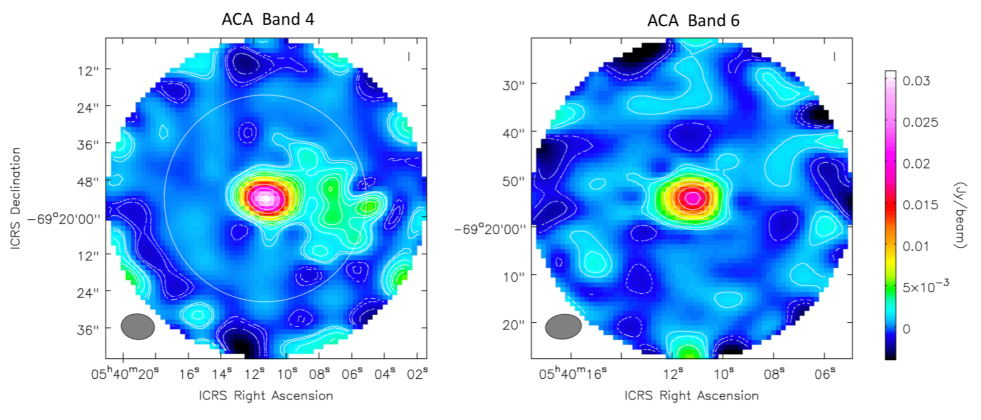
Figure 1: ACA Band 4 (left panel) and Band 6 (right panel) images of SNR 0540-69.3. The rms noise levels are 0.291 mJy and 0.348 mJy, for Bands 4 and 6, respectively. The signal-to-noise (peak flux density divided by rms) for the central part of the PWN in Band 4 is $\approx 106$, and for Band 6 it is $\approx 56$. For Band 4 the western part of the remnant shell at $20\arcsec-35\arcsec$ from the center is clearly visible. Structures at the edges of the maps are not real. The faintest intensity shown by solid white contours marks the 3$\sigma$ intensity level. The Band 4 contours shown are at -7, -4, -3, 3, 4, 7, 10, 12, 15, 20, 50, 70, 90, 100$\sigma$, and the Band 6 contours are at -5, -3, 3, 5, 10, 15, 20, 30, 40, 50$\sigma$. The ACA Band 4 beam has size $10\hbox{$.\!\!^{\prime\prime}$}79\times 8\hbox{$.\!\!^{\prime\prime}$}33$ and orientation PA $=84\hbox{$.\!\!^{\circ}$}09$, and the corresponding numbers for Band 6 are $7\hbox{$.\!\!^{\prime\prime}$}52\times 5\hbox{$.\!\!^{\prime\prime}$}18$ and PA $=-83\hbox{$.\!\!^{\circ}$}60$. The beams are displayed in the lower left corners of each panel. The intensity scale is the same for both panels. For comparison, the Band 6 field-of-view is highlighted as a white circle in the Band 4 image.

Table 2: ACA continuum parameters for SNR 0540-69.3.

Band	Frequency	$S_{\nu,{\rm peak}}$a	$\sigma_{\rm rms}$	$\theta_{\rm beam}$b
	GHz	mJy beam-1	mJy	size (PA)
4	145	$30.97\pm 1.58$	0.291	$10\hbox{$.\!\!^{\prime\prime}$}79\times 8\hbox{$.\!\!^{\prime\prime}$}33~{}(84\hbox{$.\!\!^{\circ}$}09)$
6	223.5	$19.33\pm 1.96$	0.348	$7\hbox{$.\!\!^{\prime\prime}$}52\times 5\hbox{$.\!\!^{\prime\prime}$}18~{}(-83\hbox{$.\!\!^{\circ}$}60)$

^aPeak flux density. Uncertainties are the rms noise level given in column 4, combined with a 5% absolute flux calibration uncertainty for Band 4, and a 10% uncertainty for Band 6 (cf. Section 3.2).
^bSynthesized beam size (and beam position angle, see Section 2.2)).

Table 3: Spatial resolution of the ACA, AKARI and ATCA data for SNR 0540-69.3.

Instrument	Band	Frequency	Beam size
		GHz
ATCA	3 cm	8.64	$0\hbox{$.\!\!^{\prime\prime}$}8$a
ACA	Band 4	145	$10\hbox{$.\!\!^{\prime\prime}$}79\times 8\hbox{$.\!\!^{\prime\prime}$}33$b
ACA	Band 6	223.5	$7\hbox{$.\!\!^{\prime\prime}$}52\times 5\hbox{$.\!\!^{\prime\prime}$}18$b
AKARI	MIR-L L24	$1.30\times 10^{4}$	$6\hbox{$.\!\!^{\prime\prime}$}8$c
AKARI	MIR-L L15	$1.92\times 10^{4}$	$5\hbox{$.\!\!^{\prime\prime}$}7$c
AKARI	MIR-S S11	$2.84\times 10^{4}$	$4\hbox{$.\!\!^{\prime\prime}$}8$c
AKARI	MIR-S S7	$4.16\times 10^{4}$	$5\hbox{$.\!\!^{\prime\prime}$}1$c
AKARI	NIR N3	$9.55\times 10^{4}$	$4\hbox{$.\!\!^{\prime\prime}$}0$c

^aSynthesized beam size (cf. Dickel et al., 2002).
^bSynthesized beam size (cf. Table 2).
^cFWHM according to Onaka et al. (2007).

2.2 ACA observations

We observed the millimetre/submillimetre emission in SNR 0540-69.3 using ACA in Band 4 (145 GHz) and Band 6 (223.5 GHz) as part of Atacama Large Millimeter/submillimeter Array (ALMA) program 2017.1.01391.S. The data were obtained on 2018 March 19 and 2018 March 25 for Bands 4 and 6, respectively, and the array consisted of 10–11 7-m antennas. A single pointing was observed in each band. The total on-source integration times were 438.5 seconds and 665.3 seconds, in Bands 4 and 6, respectively. The spectral setup covered a total usable bandwidth of 7.5 GHz, consisting of four 2-GHz (1.875 GHz usable), 128-channel spectral windows (spws) and dual polarisation. The four spws were centred at 138, 140, 150 and 152 GHz for Band 4 and 214.5, 216.5, 230.5 and 232.5 GHz for Band 6. The observing parameters are summarized in Table 1.

The data were reduced using the Common Astronomy Software Applications (CASA) package (McMulllin et al., 2007). We used the calibrated uv-data delivered by ALMA, which was calibrated using the ALMA Pipeline, but we performed our own imaging to improve signal-to-noise and image quality (the delivered image products were under-cleaned). The calibrated Band 4 and Band 6 datasets, respectively, contained data from 10 and 9 antennas. We carried out imaging of the continuum emission, utilizing the total 7.5 GHz bandwidth, using the CASA task TCLEAN with Briggs weighting and a Robust = 0.5 weighting of the visibilities, using CASA version 5.4.0. We also performed self-calibration. For the Band 4 data, we performed several rounds of phase-only self-calibration, initially with a 300 second time interval followed by refinement with shorter time intervals down to a 30 second interval. Amplitude self-calibration was then performed with a time interval of 30 seconds. For the Band 6 data, we performed one round each of phase-only and amplitude self-calibration, with a time interval of 300 seconds. The resulting images are shown in Figure 1, and the resulting synthesized beam sizes and rms noise levels are given in Table 2. Self-calibration produced a factor of about two improvement in the S/N for the Band 4 data compared to deeper cleaning alone (and a factor of several compared to the ALMA-delivered shallow-cleaned images). For Band 6, self-calibration only produced a slight improvement (at the 20% level) in the S/N compared to our deeper cleaning alone, but the appearance of imaging artifacts was improved.

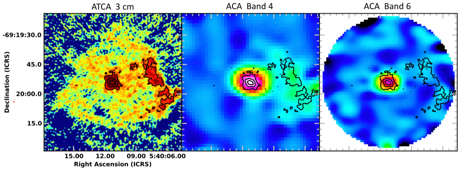
Figure 2: $70\arcsec\times 70\arcsec$ maps of PWN0540 in radio (3 cm, ATCA), and at millimetre wavelengths (2 mm and 1.3 mm, ALMA/ACA Bands 4 and 6; middle and right panels, respectively), covering the PWN and remnant shell. The axes in all three panels is the same. For comparison, and to aid the eye, contours showing the 3-cm emission at levels of 0.2, 1.0 and 2.0 mJy beam^-1 are overlaid on all the maps. In the 3-cm map the half-power beam-width is 0$.\!\!^{\prime\prime}$8 (Dickel et al., 2002), and the PWN size is $\sim 8\arcsec\times 7\arcsec$, so the PWN is fully resolved. Details for the ACA maps, including the beam sizes and intensity scale, are the same as in Figure 1. With the larger beams in the millimetre maps, the PWN is only partially resolved (see discussion in text). Note the similar structures of the western part of the remnant shell in radio and in ACA Band 4.

2.3 AKARI observations

SNR 0540-69.3 was observed in 2006 by AKARI as part of an AKARI IR survey of the Magellanic clouds (Kato et al., 2012). Five bands covered the range $2.53-28.7$ $\mu$m, which overlaps with the wavelength range of previously reported Spitzer observations (Williams et al., 2008). Processed data were retrieved from the AKARI-LMC Point Source Catalogue, and entries for PWN0540 were identified for all imaging filters in the catalogue, i.e., NIR N3 (3.2$\mu$m), MIR-S/S7 (7.0 $\mu$m), MIR-S/S11 (11 $\mu$m), MIR-L/L15 (15 $\mu$m) and MIR-L/L24 (24 $\mu$m). The observations are summarized in Table 1, and the spatial resolution in the various filter is listed in Table 3. The pixel scales in NIR, MIR-S and MIR-L images are 1$.\!\!^{\prime\prime}$446, 2$.\!\!^{\prime\prime}$340 and 2$.\!\!^{\prime\prime}$384, respectively. The photometric values in the catalogue were obtained using a radius of 10 pixels for N3, and 3 pixels for other band images. PWN0540 was therefore fully covered by the aperture photometry, although marginally so for the MIR-L/L24 band.

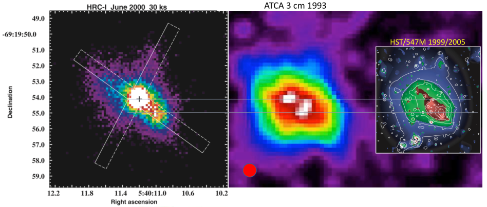
Figure 3: Zoom in of the 3-cm map (middle panel), showing two regions of strong emission (white areas), namely the pulsar region, and the “blob" $\sim 1\hbox{$.\!\!^{\prime\prime}$}5$ southwest of the pulsar. This panel is similar to that in Dickel et al. (2002), but brings out structures more clearly. The filled red circle is the 0$.\!\!^{\prime\prime}$8 HPBW. Left panel shows a Chandra 11″$\times$11″ X-ray map obtained with the High-Resolution Camera (HRC-I) in 1999. Again, the two dominating emission centres are seen. This panel, and the rightmost panel, showing the optical continuum as observed with HST/F547M, are from Lundqvist et al. (2011). Note that the HST colour map is for the 2005 epoch, and that contours are for 1999. All images are to the same scale, and grey horizontal lines have been drawn through the pulsar position, and another through the blob at its 1999 position in the optical. In the optical image, data were wavelet filtered, after the pulsar and stars had been subtracted. The position of the pulsar in this panel is marked by a black cross. See text for further details.

3 Results

3.1 Morphology revealed by ACA and ATCA

Figure 1 displays the ACA Band 4 and 6 data. The beams and their orientations are highlighted as HPBW ovals in the lower left corners of the panels, and are described in the figure caption. The central PWN is clearly seen in both bands, as well as the SNR emission to the west out to $\sim 35\arcsec$ for Band 4. Band 6 with its smaller field-of-view and lower signal-to-noise, cannot reliably trace the remnant shell (see also Figure 2).

A $70\arcsec\times 70\arcsec$ 3-cm map of SNR 0540-69.3, using the data discussed in Section 2.1, is shown in the left panel of Figure 2. Apart from the well-known strong emission on the west side, $\sim 20\arcsec-35$″ from the pulsar, there is weaker emission in a seemingly east-west symmetry. In general, the outer remnant emission is more extended on the southern side, reaching in south-eastern direction as far as it does to the south-west. The extended structure on the south-eastern side has not been revealed in previously published radio images, although emission in this region has been displayed in X-rays (Park et al., 2010). A fuller comparison between X-rays and radio for the SNR shell is made in Brantseg et al. (2014). The middle and right panels of Figure 2 show ACA Band 4 and Band 6 maps, respectively, with the 3-cm data being overlaid. The larger HPBW of the ACA data smears out the remnant structures revealed by ATCA, but there is a clear overlap of the remnant shell between radio and ACA Band 4. There is also a hint of overlap between radio and Band 6, but a deeper image is needed to draw firm conclusions.

Closing in on the PWN, both the ACA bands have beam sizes larger (Band 4), or of roughly the same size (Band 6) as the PWN. No obvious structures of the PWN are revealed in the ACA bands. This is contrasted by the detailed structure of the PWN depicted in the 3-cm radio image in the middle panel of Figure 3, where the radio image is drawn together with X-ray and optical images on the same scale. The X-ray and optical images are from our previous study in Lundqvist et al. (2011). The X-ray data were taken with Chandra HRC-I in June 2000 in the $0.2-10$ keV band, and the optical HST/F547M continuum data are from1999 and 2005, The optical data shown in Figure 3 were wavelet-filtered by Lundqvist et al. (2011) to more clearly bring out structures of the PWN.

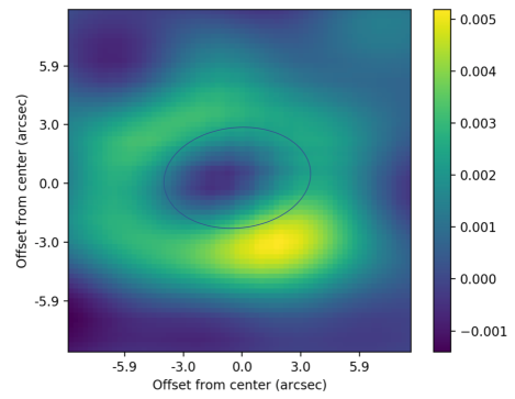
Figure 4: Difference in flux density (in Jy beam^-1) between ACA Band 6 data and a point source smeared with the $7\hbox{$.\!\!^{\prime\prime}$}5\times 5\hbox{$.\!\!^{\prime\prime}$}2$ beam (shown as an oval, see also Figure 1). The modelled point source had the same surface peak flux as in the ACA image, and was placed at the position of the peak flux density in the ACA image. The yellow/green ring-like structure is excess flux due to the extended structure of the PWN, showing that the Band 6 data are partially spatially resolved. Note the particularly strong flux density in the direction of the blob to the southwest (cf. Figure 3).

The 0$.\!\!^{\prime\prime}$8 HPBW of the radio data is shown Figure 3 as a filled red circle. The spatial resolution is good enough for the 3-cm emission to clearly reveal the two strongest continuum sources, namely the pulsar and its immediate surroundings, as well as the blob $\sim 1\hbox{$.\!\!^{\prime\prime}$}5$ southwest of the pulsar. The two centers of emission were revealed in radio for first time by Dickel et al. (2002), but there it was suggested that the pulsar was the object to the southwest. A comparison between the three panels of Figure 3 clearly shows that this is not the case, and to guide the eye, we have drawn grey horizontal lines in the east-west direction through the position of the pulsar and through the blob at its 1999 position. As discussed by De Luca et al. (2007) and Lundqvist et al. (2011), the emission centre of the blob in the optical appears to move over time towards the southwest. This is visible in the panel to the right of Figure 3 where the 1999 structure in the optical is overlaid on that from 2005. If the blob is a multi-wavelength feature/entity, it does not come as a surprise that the blob in the X-ray image from 2000 lines up well with the optical image from the same year, and that the radio image from 1995 shows a blob emission centered slightly closer to the pulsar than on images from 1999/2000. From Figure 3 this seems to be the case. However, the overall structure of the PWN is similar at all wavelengths, although the relative flux densities within the PWN vary with frequency.

3.2 Fluxes in the ACA and AKARI bands

The peak flux density of SNR 0540-69.3 in Band 4 is 30.97 mJy beam^-1 and the rms 0.291 mJy beam^-1. For Band 6 the corresponding numbers are 19.33 mJy beam^-1 and 0.348 mJy beam^-1, respectively. These and other image properties are given in Table 2. While the S/N of PWN0540 in Band 4 is $\approx 106$ after our improved cleaning and self-calibration (see Section 2.2), the S/N of the brightest pixel in the SNR shell features is $\sim$18, so it is clear that the factor of $\sim$2 improvement in S/N provided by self-calibration results in a significantly more robust detection of this extended feature (and we note that these SNR shell features were not detected in the initial shallow-cleaned images; the deeper cleaning and self-calibration described in Section 2.2 were essential for the detection of these features). Regarding uncertainties, as stated in Table 2, there is an uncertainty in the absolute flux calibration, which is estimated to be 5% for Band 4 and 10% for Band 6, as detailed in the ALMA Proposer’s Guide (Section A.9.2) and the ALMA Technical Handbook (Chapter 10). The flux uncertainty quoted in Table 2 is a combination of this and the rms.

The integrated flux density from the PWN would be the same as the peak flux density if the PWN were unresolved. This is not the case, since PWN0540 is partially resolved in both ACA bands. To test this we made an experiment were we assume that the source is a point source, so that the modeled spatial flux density distribution essentially becomes the beam distribution. We then normalized the peak flux density of this image to the observed image for each band. The difference between the observed image and the model is shown in Figure 4 for Band 6. The net flux density is at zero level in the center, as expected, but positive residuals are clearly displayed outside the HPBW oval, especially in the direction towards the blob.

We can use the result from this experiment to estimate a correction factor for the integrated flux density from the PWN, compared to the observed peak flux densities. This correction factor is simply the net flux density, as displayed in Figure 4 for Band 6, relative to that measured from a point source. We obtain the correction factors $\sim 1.19$ and $\sim 1.50$ for Bands 4 and 6, respectively. The correction factor, and its estimated uncertainty, are included in Table 4 for Band 6. The situation is more complicated for Band 4, since for this band the correction factor is affected by flux from the SNR shell being smeared into the PWN region.

For Band 4 we have therefore also made another test which relies on an assumption that the underlying structures of the PWN and the SNR shell are similar at 3 cm and in the ACA bands. This assumption is best checked for Band 6 image with its higher spatial resolution, by smearing the 3 cm image with the ACA Band 6 beam, and then subtract this from the observed ACA Band 6 image. The residuals are found to be consistent with noise, which means that the intrinsic structures are similar at 3 cm and in Band 6 (and therefore also in Band 4), at least at the levels of signal-to-noise and spatial resolution of the ACA bands.

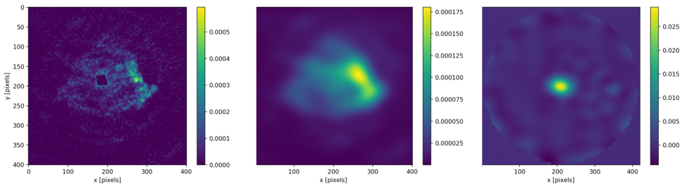
Figure 5: 3-cm image of SNR 0540-69.3, with the PWN masked out (left panel). To obtain the middle panel we smeared the 3-cm image with the ACA Band 4 beam. This simulates the structure of the pure remnant shell in Band 4, and is named Image_4shell in Section 3.2. The image in the panel to the right is the observed ACA Band 4 shown in the left panel of Figure 1 (and called Image_4obs in Section 3.2) minus Image_4shell. The fux densities are in Jy beam^-1.

This intrinsic similarity between radio and millimetre structures allows us to improve on the correction for the integrated flux density of the PWN in Band 4. We did this by first constructing two images. For the first image we only considered the PWN area of the 3-cm map, and smeared this with the ACA Band 4 beam. We call this Image_4PWN. We also made a simulated image of the SNR shell, Image_4shell, where we first masked out the PWN from the 3-cm map, and then smeared the rest with the ACA Band 4 beam. We show this process in Figure 5. We then removed the simulated shell image Image_4shell from the observed Band 4 image, Image_4obs, thereby creating the right panel of Figure 5. This last step can be written

$$\text{Image}_{4\text{diff}}=\text{Image}_{4\text{obs}}-B\times\text{Image}_{4\text{SNR}}~{}.$$ (1)

We then created a null image by removing Image_4PWN from Image_4diff, i.e.,

$$\text{Image}_{4\text{resid}}=\text{Image}_{4\text{diff}}-A\times\text{Image}_{4\text{PWN}}~{}.$$ (2)

The difference was tuned through the constants $A$ and $B$ to achieve zero net flux density at the positions of the PWN and SNR, respectively. The ratio $A/B$ can be used to estimate a power-law index for the spectral range between 3 cm and ACA Band 4 for the SNR shell emission, if the index is known for the PWN.

$$\alpha_{\nu,\text{SNR}}=\alpha_{\nu,\text{PWN}}+0.816~{}\text{lg}(A/B).$$ (3)

In our analysis we arrive at $A/B=3.8\pm 0.2$, so that $\alpha_{\nu,\text{SNR}}-\alpha_{\nu,\text{PWN}}=0.47\pm 0.03$. Brantseg et al. (2014) estimated $\alpha_{\nu,\text{SNR}}-\alpha_{\nu,\text{PWN}}=0.50\pm 0.04$ for radio alone. Our result is fully consistent with the same difference in power-law index continuing into the millimetre regime.

The peak flux density of the image in the right panel of Figure 5, i.e., Image_4diff, is 29.07 mJy beam^-1, which is $\sim 6\%$ lower than before the correction for emission from the remnant shell (cf. Table 2). Finally, we used Image_4diff to calculate the flux correction factor for the PWN, as we did for Band 6, to arrive at the value $1.05$, which we include in the integrated flux density for Band 4 in Table 4. This correction factor is smaller than the value we obtained before compensating for the SNR shell, as expected.

For the AKARI data, we used 343.34, 74.956, 38.258, 16.034, and 8.0459 Jy as fluxes for zero magnitude for the five IRC bands N3, S7 S11, L15 and L24, respectively (Tanabé et al., 2008; Kato et al., 2012). The AKARI flux densities are listed in Table 4, along with the frequency interval for which the normalized filter transparency is $\geq 50\%$.

Table 4: Observed multi-wavelength integrated flux densities of PWN0540.^a

Frequency	Instrument	Flux density	Sourceb
GHz		mJy
$1.513\pm 0.064$	ATCA 20 cm	$68\pm 7$c	1
$2.290\pm 0.064$	ATCA 13 cm	$62\pm 6$c	1
$4.790\pm 0.064$	ATCA 6 cm	$54\pm 5$c	1
$5.824\pm 0.064$	ATCA 6 cm	$60\pm 6$c	1
$8.640\pm 0.064$	ATCA 3 cm	$51\pm 5$c	1
$145.0\pm 7.9$	ACA Band 4	$30.5\pm 1.6$c,d	2
$223.5\pm 9.9$	ACA Band 6	$29.1\pm 3.0$c	2
$4350\pm 110$	Spitzer MIPS Ch2	$<366$	3
$(1.26\pm 0.21)\times 10^{4}$	Spitzer MIPS Ch1	$13.19\pm 3.95$	3
$(1.30\pm 0.15)\times 10^{4}$	AKARI MIR-L L24	$17.9\pm 1.2$	2
$(1.92\pm 0.36)\times 10^{4}$	AKARI MIR-L L15	$6.29\pm 1.02$c	2
$(2.84\pm 0.54)\times 10^{4}$	AKARI MIR-S S11	$4.62\pm 0.27$c	2
$(3.94\pm 0.73)\times 10^{4}$	Spitzer IRAC Ch4	$5.10\pm 0.74$c	3
$(4.16\pm 0.50)\times 10^{4}$	AKARI MIR-S S7	$3.38\pm 0.24$c	2
$(5.31\pm 0.66)\times 10^{4}$	Spitzer IRAC Ch3	$3.61\pm 0.46$c	3
$(6.76\pm 0.76)\times 10^{4}$	Spitzer IRAC Ch2	$2.19\pm 0.27$c	3
$(8.54\pm 0.90)\times 10^{4}$	Spitzer IRAC Ch1	$1.77\pm 0.23$c	3
$(9.55\pm 1.70)\times 10^{4}$	AKARI NIR N3	$2.26\pm 0.20$c	2
$(1.41\pm 0.12)\times 10^{5}$	VLT/NACO/$K_{s}$	$0.801\pm 0.035$c	4
$(1.83\pm 0.19)\times 10^{5}$	VLT/NACO/$H$	$0.675\pm 0.027$c	4
$(2.36\pm 0.20)\times 10^{5}$	VLT/NACO/$J$	$0.541\pm 0.022$c	4
$(3.68\pm 0.57)\times 10^{5}$	HST/F814We	$0.481\pm 0.014$	4
$(3.76\pm 0.43)\times 10^{5}$	HST/F791W	$0.437\pm 0.009$c	5
$(3.76\pm 0.43)\times 10^{5}$	HST/F791W	$0.426\pm 0.013$c	4
$(4.48\pm 0.43)\times 10^{5}$	HST/F675Wf	$0.472\pm 0.018$	4
$(5.50\pm 0.36)\times 10^{5}$	HST/F547M	$0.267\pm 0.005$c	5
$(5.71\pm 0.86)\times 10^{5}$	HST/F555Wg	$0.346\pm 0.017$	4
$(6.89\pm 1.13)\times 10^{5}$	HST/F450Wh	$0.361\pm 0.022$	4
$(9.00\pm 0.64)\times 10^{5}$	HST/F336W	$0.124\pm 0.002$	5
$(9.00\pm 0.64)\times 10^{5}$	HST/F336W	$0.211\pm 0.022$c	4

^aNear-infrared observations, and observations at higher frequencies, are dereddened integrated flux densities, according to their sources.
^bReferences: (1) Brantseg et al. (2014), (2) This paper, (3) Williams et al. (2008), (4) Mignani et al. (2012), (5) Serafimovich et al. (2004).
^cIncluded in the power-law fits in Figures 6 and 7
^dIncludes correction for extended emission from the SNR shell.
^eIncludes [S iii] $\lambda\lambda 9069,9532$.
^fIncludes [N ii] $\lambda\lambda 6548,6583$, H$\alpha$ and [S ii] $\lambda\lambda 6716,6731$.
^gIncludes [O iii] $\lambda\lambda 4959,5007$.
^hIncludes [O ii] $\lambda\lambda 3726,3729$ and [O iii] $\lambda\lambda 4959,5007$.

4 Discussion

We have used integrated flux densities in Table 4 to fit power-laws to different parts of the synchrotron spectrum. Not all data in the table have been included in these fits, as will be detailed below. Concentrating first on the radio/mm-region, we have used the ACA flux densities in Section 3.2 together with radio flux densities from Brantseg et al. (2014). We note that there is some inconsistency in Brantseg et al. (2014) with regard to the 6-cm flux densities at 4.790 GHz and 5.824 GHz in their Figures 6 and 11, compared to their Table 2. We have assumed that the flux densities in their Table 2 are correct (since they agree with their Figure 11), and have used the flux densities uncertainties shown in their Figure 6 (as no uncertainties are provided in their Table 2). With this caveat in mind, we estimate $\alpha_{\nu}=0.17\pm 0.02$ for the frequency interval $1.449-233.50$ GHz. This is shown in Figure 6.

The uncertainty of $\alpha_{\nu,{\rm radio/mm}}$ and its 1$\sigma$ interval were estimated using the same method as in Serafimovich et al. (2004), i.e., utilizing a Monte Carlo approach to construct 10 000 power-laws to fit 10 000 simulated sets of data, where the flux uncertainty is assumed to have a Gaussian distribution, and the frequency distribution to be evenly distributed within the frequency bins given in Table 4. We have then ordered the 10 000 simulated data sets in order of fitted $\alpha_{\nu,{\rm radio/mm}}$ values, and from this assigned the median value to be the preferred $\alpha_{\nu,{\rm radio/mm}}$. We did this 500 times with different seed values for the randomizer, and then took the average value for the power-law index to be the final estimate of the index. The 1$\sigma$ boundaries for $\alpha_{\nu,{\rm radio/mm}}$ shown in Figure 6 come from the constraint that 68% of the constructed power laws must lie within the 1$\sigma$ boundaries.

To make a similar fit to the IR/UV part of the spectrum, we included the Spitzer IRAC IR data from Williams et al. (2008), the AKARI data in Table 4 and the VLT/NACO data of Mignani et al. (2012). HST data for PWN0540 in the optical/UV have been published by Serafimovich et al. (2004) and Mignani et al. (2012). In Serafimovich et al. (2004) care was taken to only consider HST filters which do not include strong nebular spectral lines. On the contrary, most of the filters considered by Mignani et al. (2012) include the strongest lines in the nebula (cf. Kirshner et al., 1989; Serafimovich et al., 2005; Morse et al., 2006), as we have indicated in Table 4. To check the contribution from spectral lines to the flux in HST filters, we have chosen to study the influence by [O iii] $\lambda\lambda$4959,5007 on the flux in F555W. Fluxes for various lines from the whole PWN were estimated by Williams et al. (2008). For [O iii] $\lambda$5007 they used the line flux deduced by Morse et al. (2006), and assumed that the size of the PWN, as seen in [O iii], is a factor of $\approx 4$ larger than the area covered by the slit used by Morse et al. (2006). This means that the dereddened line flux from the whole PWN is $f_{[\text{O\,{iii}}]\lambda 5007}\approx 2.7\times 10^{-13}~{}{\rm erg~{}cm}^{-2}~{}{\rm s}^{-1}$. However, the slit used by Morse et al. (2006) covers the brightest areas in [O iii] (cf. Sandin et al., 2013), so a correction factor of 4 is too large. We have taken a more conservative approach for the flux of [O iii] $\lambda\lambda$4959,5007 than Williams et al. (2008), and adopt $f_{[\text{O\,{iii}}]\lambda 5007}=2.0\times 10^{-13}~{}{\rm erg~{}cm}^{-2}~{}{\rm s}^{-1}$ and $f_{[\text{O\,{iii}}]\lambda 4959}$ to be one third of that, in accordance with the 3:1 ratio of the transition probabilities of the two lines (e.g., Osterbrock & Ferland, 2006). To compare with the continuum emission, we use the flux in the F547M filter (cf. Table 4) and the continuum spectral slope $F_{\nu}\propto{\nu}^{-0.87}$ (see below). With the filter transmission considered, we arrive at an [O iii] $\lambda\lambda$4959,5007 flux which is $\sim 60$% of the continuum flux within F555W, i.e, the integrated continuum flux density at $5.71\times 10^{14}$ Hz, is probably closer to $0.20-0.25$ mJy than the $\sim 0.35$ mJy listed in Table 4. Had we used the [O iii] $\lambda$5007 line flux estimated by Williams et al. (2008), the derived ntegrated continuum flux density in F555W would have been $\!\!\!\phantom{\leq}\smash{\buildrel\over{\lower 2.67502pt\hbox{$\buildrel\lower 2.14001pt\hbox{$\displaystyle<$}\over{\sim}$}}}\,\,0.20$ mJy. Based on this, we have discarded HST filters which encapsulate strong nebular lines from our analysis.

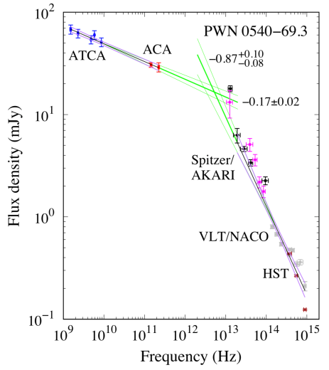
Figure 6: Multi-wavelength spectrum of PWN0540. Our estimated flux densities in ACA Bands 4 and 6 are shown by red symbols, and the radio flux densities estimated by Brantseg et al. (2014) are marked in blue. The best power-law fit to those data has a spectral index of $\alpha_{\nu,{\rm mm}}=0.17\pm 0.02$. (The figure gives spectral slopes, i.e., $-\alpha_{\nu}$.) A similar fit to the UV/IR part gives $\alpha_{\nu,{\rm UVIR}}=0.87^{+0.08}_{-0.10}$. 1$\sigma$ intervals for the power-laws are drawn in purple. The data included in this fit are the Spitzer IRAC data of Williams et al. (2008) (in magenta), AKARI data reported here (in black), and the VLT/NACO data of Mignani et al. (2012) (in grey). Data for the UV/optical regime published by Serafimovich et al. (2004) (in brown) and by Mignani et al. (2012) (in grey) are all shown in the figure, but as detailed in the text, not all those data were included in the power-law fit. Extrapolations of the two power-laws (in green), intersect at $\nu\sim 5.2\times 10^{12}$ Hz. Extrapolations of the 1$\sigma$ intervals are also drawn in green.

The HST filters we have included are F336W, F547M and F791W. For F791W, the fluxes estimated by Serafimovich et al. (2004) and Mignani et al. (2012), using the same data from 1999 October 17, agree to within 3%, and we used an average value of those. This contrasts the situation for F336W where the two teams obtained very different results. Mignani et al. (2010, 2012) argue that this is not mainly because the groups analyze different data sets (from 1999 October 17 and 2007 June 21), but that the so-called Charge Transfer Efficiency (CTE) effect, which is important for F336W, is treated better by them. We have therefore chosen to only include the Mignani et al. (2012) measurement for that filter. F547M does not include any strong nebular lines (Serafimovich et al., 2004), and this band was included in our power-law estimate. All data used in our power-law fits are highlighted in Table 4 by the asterisk marked “c”. With this in mind, we arrive at $\alpha_{\nu,{\rm UVIR}}=0.87^{+0.08}_{-0.10}$ for the IR/UV part of the synchrotron spectrum. (Had we included the F336W flux of Serafimovich et al., 2004, the power-law index would only have changed to $0.91^{+0.08}_{-0.10}$.) This is less steep than $\alpha_{\nu}=1.48^{+0.09}_{-0.08}$ by Serafimovich et al. (2004) and $1.27\pm 0.3$ by Brantseg et al. (2014), but steeper than $\alpha_{\nu}=0.56\pm 0.03$ by Mignani et al. (2012). Our results supersede all those estimates. The $-0.87^{+0.10}_{-0.08}$ spectral slope for the IR/UV range is drawn and marked in Figure 6. Note the flux excess for the discarded HST filters compared to the power-law fit, due to line emission contamination.

In the IR, the integrated AKARI flux densities in the range $(2.3-4.7)\times 10^{13}$ Hz are lower than those measured by Spitzer, despite the fact that there is line contribution mainly from to [S iv] 10.5 $\mu$m (Williams et al., 2008, see also Figure 8). This underlines difficulties in background subtraction in the IR. In general, the AKARI data line up better with the full IR/UV power-law, except for the N3 and L24 bands. The L24 band is not part of the power-law fits in Figure 6 though.

In Figure 6, an extrapolation of the high-energy power-law undershoots the flux level of the $\sim 24~{}\mu$m AKARI data by several $\sigma$. This could signal a contribution to the emission from dust with $T_{\rm dust}\sim 40-65$ K, as argued for by Williams et al. (2008). However, broad-line emission in [C iv] 25.9 $\mu$m and [Fe ii] 26.0 $\mu$m contributes to the integrated AKARI flux density in AKARI L24 band. Using the line fluxes estimated by Williams et al. (2008), and taking into account the transparency in the L24 band at 26 $\mu$m, we estimate that lines can contribute up to $\sim 5-6$ % of the integrated AKARI flux density in the L24 band, which only marginally decreases the need for dust to fit the $24~{}\mu$m data (see below).

Extrapolations of the low-frequency and the IR/UV power-laws in Figure 6 intersect at $\nu_{\rm break}\sim 5.2\times 10^{12}$ Hz. If we use the 1$\sigma$ limits in Figure 6 we obtain $\nu_{\rm break}=(5.2^{+3.6}_{-2.8})\times 10^{12}$ Hz. If one assumes that this break is due to synchrotron cooling of relativistic electrons, one can estimate the magnetic field strength, $B$, where the electrons are being injected. Equalling the life-time of synchrotron-emitting electrons, $\tau_{\rm synch}=6\times 10^{11}B^{-3/2}\nu_{\rm break}^{-1/2}$ s (Pacholczyk, 1970; Brantseg et al., 2014), to the age of the remnant, assumed to be 1 100 years (Reynolds, 1985), this translates into $B=(3.9^{+1.1}_{-0.7})\times 10^{-4}$ G. This is higher than the findings of Manchester et al. (1993b) and Brantseg et al. (2014), who both estimated $B\sim 2.5\times 10^{-4}$ G, but somewhat lower than a recent value derived from X-rays, $B=(7.8^{+45}_{-2.8})\times 10^{-4}$ G (Ge et al., 2019).

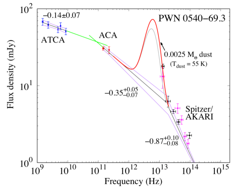
Figure 7: Same as Figure 6, but only showing the ATCA, ACA, Spitzer and AKARI data. One separate power-law fit has been made for the ATCA data, and another for the ACA data plus the AKARI 15 $\mu$m data. Spectral indices for the various frequency intervals are shown ($\alpha_{\nu,{\rm radio}}=0.14\pm 0.07$ and $\alpha_{\nu,{\rm mm/IR}}=0.35^{+0.07}_{-0.05}$). (The figure gives spectral slopes, i.e., $-\alpha_{\nu}$.) Extrapolations of the radio–IR power-laws intersect at $\sim 8.4\times 10^{10}$ Hz, which can compared with a similar break at $\sim 3\times 10^{10}$ Hz break for the Crab Nebula. Emission from $2.5\times 10^{-3}~{}{\rm M}_{\odot}$ of silicate dust with temperature $T_{\rm dust}=55$ K is also included (in red), to model the AKARI and Spitzer data long-ward of $\sim 20~{}\mu$m. For a comparison we also include a model (in grey) with preferred values by Williams et al. (2008), namely the dust mass $3\times 10^{-3}~{}{\rm M}_{\odot}$ and $T_{\rm dust}=50$ K.

The spectral break between the low- and high frequency parts of the synchrotron spectrum gives a steepening in power-law index by $\Delta=0.70^{+0.08}_{-0.10}$, which is slightly larger than the expected standard change of 0.5 due to synchrotron losses in a homogeneous medium. Although $\Delta=0.5$ is not fully excluded from our spectral fits, Reynolds (2009) discusses possibilities with $\Delta>0.5$, and how this could signal inhomogeneities in regions where the relativistic electrons are injected. There is also the possibility that the $\Delta\sim 0.7$ break in power-law index is not due to synchrotron losses, but signals two populations of relativistic electrons, as in the model of Bucciantini et al. (2011, cf. Introduction).

Rather than a single power-law break at $\nu_{\rm break}\sim 5.2\times 10^{12}$ Hz, a dual break is also possible. The Crab PWN may serve as a template. As described in the Introduction, the Crab PWN has a spectral break at $\sim 3\times 10^{10}$ Hz, where the spectral index changes from $\alpha_{\nu}\approx 0.3$ in the radio to $\alpha_{\nu}\approx 0.42$ at higher frequencies (Gomez et al., 2012). There could be a similar break for PWN0540. If we fit a power-law to the radio data alone, the spectral index becomes $\alpha_{\nu,{\rm radio}}=0.14\pm 0.07$. Similarly, we can also fit a power-law to the ACA data and the AKARI L15 data at $(1.92\pm 0.36)\times 10^{13}$ Hz, and the power-law for this range then is $\alpha_{\nu,{\rm mm/IR}}=0.35^{+0.07}_{-0.05}$. As shown in Figure 7, the two power-laws intersect at $\sim 8.4\times 10^{10}$ Hz, i.e., somewhat higher frequency than the $\sim 3\times 10^{10}$ Hz break for the Crab. With dual power-laws, the total steepening in power-law index becomes $\Delta=0.73^{+0.11}_{-0.12}$, which is again greater than $\Delta=0.5$ at $\sim 2\sigma$ level.

However, the difference in power-law index between $\alpha_{\nu,{\rm mm/IR}}$ and $\alpha_{\nu,{\rm UVIR}}$ is $0.52\pm 0.11$, which is fully consistent with a cooling break of 0.5. Returning to the model of Bucciantini et al. (2011, see also ()), there could be two populations of relativistic electrons, one being responsible for radio emission, and the other giving rise to the mm/IR part. The latter could experience a break due to synchrotron losses, which is reflected in a power-law break of $\sim 0.5$ at $\nu_{\rm break}\sim 2\times 10^{13}$ Hz. If we use $B=8\times 10^{-4}$ G, as indicated from X-rays, $\tau_{\rm synch}\sim 190$ years, which is markedly less than the age of the remnant, although not as low as $\tau_{\rm synch}\sim 2.6$ years estimated by Petre et al. (2007), from a presumed cooling break in X-rays instead of at $\sim 2\times 10^{13}$ Hz. Inspired by the model of Lyutikov et al. (2019), which suggests a cooling break at $\sim 0.01$ eV for the Crab PWN, $\tau_{\rm synch}\sim 190$ years seems more likely than $\sim 3$ years for PWN0540.

A dual spectral break in the radio-IR range for the synchrotron emission in PWN0540 as shown in Figure 7 allows for the possibility of dust emission to explain excess emission at 24 $\mu$m. Such a dust component was discussed by Williams et al. (2008), and in Figure 7 we include emission (shown in red, and highlighted with a black arrow) from $2.5\times 10^{-3}~{}{\rm M}_{\odot}$ of silicate dust with a temperature of $T_{\rm dust}=55$ K (red solid line). The dust emission was calculated assuming optically thin forsterite dust. The flux density $F_{\lambda}$ at wavelength $\lambda$ can be written as

$$F_{\lambda}=\frac{\kappa_{\lambda}M_{\rm dust}B_{\lambda}(T_{\rm dust})}{D^{2}}~{},$$ (4)

where $M_{\rm dust}$ is the dust mass, $D$ the distance to PWN0540 (i.e., 50 kpc), $B_{\lambda}(T_{\rm dust})$ the Planck function for temperature $T_{\rm dust}$, and $\kappa_{\lambda}\propto\lambda^{-\beta}$ the mass absorption coefficient of the selected type of dust (e.g., Hildebrand, 1983; Matsuura, 2017). The values of $\kappa_{\lambda}$ and $\beta$ are temperature dependent. We have assumed small-sized dust particles, and interpolated $\kappa_{\lambda}$ and $\beta$ in temperature using the results reported by Mennella et al. (1998). The choice of silicate dust is motivated by the fact that Nozawa et al. (2003) find that silicates may dominate in supernova ejecta of massive progenitors, especially in mixed ejecta. Williams et al. (2008) show that the presumed dust component increases in strength towards longer wavelengths up to the end of their spectra at $\sim 37~{}\mu$m. This is consistent with the model in Figure 7 where the curve in red (dust + synchrotron) peaks at $\sim 50~{}\mu$m. Our dust mass estimate is consistent with the $\sim 3\times 10^{-3}~{}{\rm M}_{\odot}$ of silicate dust with $T_{\rm dust}=50\pm 8$ K calculated by Williams et al. (2008). In Figure 7 we include (in grey) a model with those parameters. As can be seen, this model does not fit the integrated AKARI L24 flux density well. This is not surprising since the model of Williams et al. (2008) was tuned to fit Spitzer data. The inclusion of the AKARI L24 data pushes the derived dust temperature to a slightly higher value than estimated by Williams et al. (2008).

As can be seen in Figure 7, the AKARI and Spitzer flux densities are larger than the extrapolation along the best optical–IR synchrotron fit. This could indicate a dust contribution all the way up in frequency to the VLT/NACO bands, i.e., up to $\sim 1.4\times 10^{14}$ Hz. This would require dust temperatures ranging between $\sim 50-60$ K, or lower, and up to several hundred Kelvins. Although warm dust is seen in SNe (cf. Matsuura, 2017, and references therein), detected PWN-embedded dust usually has temperatures lower than 100 K (Chawner et al., 2019). SNR 1E 0102.2-7219 in the Small Magellanic Cloud (SMC) may be an exception at first glance. Sandstrom et al. (2009) argue that small amounts ($\sim 2\times 10^{-5}\hbox{M${}_{\odot}$}$) of newly formed forsterite dust with $T_{\rm dust}\approx 140$ K is associated with the supernova ejecta, and a pulsar was recently reported for this remnant. However, no PWN (Vogt et al., 2018) has yet been found, so SNR 1E 0102.2-7219 is probably more similar to Cas A than PWN0540 when it comes to the central source and its immediate surroundings.

A more likely reason for the high AKARI and Spitzer flux densities $\!\!\!\phantom{\leq}\smash{\buildrel\over{\lower 2.67502pt\hbox{$\buildrel\lower 2.14001pt\hbox{$\displaystyle<$}\over{\sim}$}}}\,\,20\mu$m is line contribution. For example, as shown in Figure 8, the AKARI S11 band observations of PWN0540 (Williams et al., 2008) include [S iv] 10.5 $\mu$m at $f_{[\text{S\,{iv}}]}\approx 7.3\times 10^{-14}~{}{\rm erg~{}cm}^{-2}~{}{\rm s}^{-1}$, and [Ne ii] 12.8 $\mu$m at $f_{[\text{Ne\,{ii}}]}\approx 5.0\times 10^{-14}~{}{\rm erg~{}cm}^{-2}~{}{\rm s}^{-1}$. In Figure 8, the blue solid line is part of the $\alpha_{\nu,{\rm UVIR}}=0.87$ power-law fit in Figures 6 and 7, and the fluxes of the spectral lines are the broad lines (FWHM $\sim 1000~{}\mbox{\,km s${}^{-1}$}$) reported by Williams et al. (2008). Taking into account the transmission of the AKARI S11 filter (cf. Figure 8), the measured flux in the spectral lines is $\sim 20\%$ of the continuum flux. If we add this estimated line contribution to the power-law fit value for the continuum in the AKARI S11 band, which is $3.81$ mJy at at $2.84\times 10^{13}$ Hz, the total flux density becomes $4.57$ mJy. This agrees excellently with the observed integrated flux density in the AKARI S11 band which is $4.62\pm 0.27$ mJy (cf. Table 4).

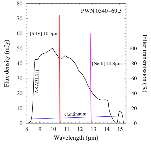
Figure 8: Emission from PWN0540 in the AKARI S11 band. The blue solid line is a power-law fit to the synchrotron continuum, adopting the $\alpha_{\nu,{\rm UVIR}}=0.87$ power-law index from Figures 6 and 7. The two strongest spectral lines in this band, [S iv] 10.5 $\mu$m and [Ne ii] 12.8 $\mu$m, are also shown. Fluxes and widths of the lines are from Williams et al. (2008). The normalized filter transmission of the S11 band is highlighted by the black solid line. See text for further details.

In our flux estimates of the continuum emission from PWN0540, we have made no correction for emission from PSR0540. Serafimovich et al. (2004) made a detailed discussion of this for the optical/UV part, and their results indicate that the pulsar would contribute $\sim 5$% if the pulsar were not spatially resolved. The multi-wavelength compilation of Serafimovich et al. (2004) also show that the PWN and the pulsar are of equal strength in X-rays (cf. Figure 3), but that in radio the pulsar contribution is negligible compared to that from the PWN. This trend is confirmed by Mignani et al. (2012) whose results point to a $\sim 3$% pulsar contribution in the $H$ band. We can therefore safely ignore any pulsar contribution to the integrated flux densities in the ACA, AKARI and Spitzer bands. As outlined before, uncertainties due to spectral lines are larger. Further observations of PWN0540 in the near- and mid-infrared, preferably spectroscopic to remove the flux from spectral lines, should solve whether dust contributes to the emission measured by Spitzer and AKARI. For example, the James Webb Space Telescope (JWST), with its expected spectral range between $0.6-28.5~{}\mu$m and 0$.\!\!^{\prime\prime}$1 optical spatial resolution, is an ideal tool for this task.

In our analysis in Section 3.2 we obtained $\alpha_{\nu,\text{SNR}}-\alpha_{\nu,\text{PWN}}=0.47\pm 0.03$ for the difference in spectral index between the remnant shell and the PWN for the spectral interval $8.6-145$ GHz. Using Table 4 we find $\alpha_{\nu,\text{PWN}}=0.19{\pm 0.04}$, and hence $\alpha_{\nu,\text{SNR}}=0.64{\pm 0.05}$. Brantseg et al. (2014) found $\alpha_{\nu,\text{SNR}}=0.65{\pm 0.01}$ for the range $1.4-8.6$ GHz, fully consistent with a constant spectral slope over two orders of magnitude in frequency. Our value for the remnant shell is also consistent with typical values for synchrotron radiation from other radio SNRs (Green, 2009). It is also consistent with the spectrum for the synchrotron emission from the circumstellar ring around SN 1987A where $\alpha_{\nu,\text{87A}}=0.70{\pm 0.06}$ (Cigan et al., 2019) for the same extended frequency interval we have discussed for SNR 0540-69.3 (see also Zanardo et al., 2014).

5 Conclusions

We have observed SNR 0540-69.3 with the Atacama Compact Array (ACA) in Bands 4 (137–153 GHz) and 6 (213.5–233.5 GHz), which is a new frequency range for this object. As the half-power beam-width (HPBW) of ACA is similar to the size of the remnants pulsar-wind nebula (PWN) in Band 6 ($7\hbox{$.\!\!^{\prime\prime}$}5\times 5\hbox{$.\!\!^{\prime\prime}$}2$), and slightly larger than the PWN in Band 4 ($10\hbox{$.\!\!^{\prime\prime}$}8\times 8\hbox{$.\!\!^{\prime\prime}$}3$), the PWN was only partially resolved.

We also use deep radio observations obtained with the Australia Compact Array (ATCA) at 3 cm, with an HPBW of $\approx 0\hbox{$.\!\!^{\prime\prime}$}8$. We used the 3-cm data as a template for the emission in the millimeter-range, and smeared these data with the HPBWs of ACA Bands 4 and 6. These simulations suggest a similar overall structure at millimetre wavelengths compared to that at 3 cm. In particular, we recover the strong emission $\sim 1\hbox{$.\!\!^{\prime\prime}$}5$ to the south-west of the pulsar seen at other wavelengths. If we include published radio flux densities (Brantseg et al., 2014), we obtain a synchrotron spectrum $F_{\nu}\propto\nu^{-0.17\pm{0.02}}$ for the frequency interval $1.449-233.50$ GHz.

To draw conclusions about how the radio-millimetre wavelength range of the spectrum joins to the synchrotron spectrum at higher frequencies, and whether there could be dust in the PWN, we have evaluated published data in the UV, optical and IR, as well as included previously unpublished AKARI IR data. We show that some of these data are seriously contaminated by spectral line emission, and are therefore not suitable for analyzing the continuum emission. For the UV/IR part of the synchrotron spectrum, we find $F_{\nu}\propto\nu^{-0.87^{+0.10}_{-0.08}}$. The break between the radio–millimetre and UV/IR power-law occurs at $\nu_{\rm break}=(5.2^{+3.6}_{-2.7})\times 10^{12}$ Hz, which can be used to estimate the magnetic field strength, $B=(3.9^{+1.1}_{-0.7})\times 10^{-4}$ G, in the PWN, if the lifetime of synchrotron-emitting electrons is as large as the remnant age. This field strength is slightly higher than previous findings of Manchester et al. (1993b) and Brantseg et al. (2014).

To explain the high observed flux from the PWN at $24~{}\mu$m, and at the same allow for a break in the synchrotron spectrum between radio and millimetre wavelengths as is seen in the Crab, we find that dust with a temperature of $\sim 50-60$ K is needed. For 55 K, the mass is $\sim 2.5\times 10^{-3}~{}{\rm M}_{\odot}$ for forsterite dust. The inferred break between radio and millimetre wavelenghts would occur at $\sim 8\times 10^{10}$ Hz, with the spectral slope changing from $-0.14\pm 0.07$ in the radio, to $-0.35^{+0.05}_{-0.07}$ in the millimetre to far-IR range. The total change in power-law index based between radio and the optical/UV is $\Delta\sim 0.7$, with $\Delta=0.5$, as in the standard case of synchrotron losses in a homogeneous medium, being excluded at $\sim 2\sigma$ level, regardless of whether there is a spectral break at $\sim 8\times 10^{10}$ Hz, or not.

However, there is a possible scenario for PWN0540, which is inspired by a recent model by Lyutikov et al. (2019) for the Crab PWN, and which can accommodate a cooling break of $\sim 0.5$. In this model our spectra reveal two populations of synchrotron-emitting relativistic electrons: one that emits in the radio with $F_{\nu}\propto\nu^{-0.14\pm 0.07}$, and another that emits in the millimetre to UV range. In the millimetre to far-IR range, the latter component emits according to $F_{\nu}\propto\nu^{-0.35^{+0.05}_{-0.07}}$. Although shallower than $\propto\nu^{-0.5}$, uncertainties are large enough for this component to be consistent with Fermi acceleration. The observed steepening in power-law index by $0.52\pm 0.11$ to $F_{\nu}\propto\nu^{-0.87^{+0.10}_{-0.08}}$ for $\nu\!\!\!\phantom{\geq}\smash{\buildrel\over{\lower 2.67502pt\hbox{$\buildrel\lower 2.14001pt\hbox{$\displaystyle>$}\over{\sim}$}}}\,\,2\times 10^{13}$ Hz could be due to synchrotron cooling, as in the Crab. For a magnetic field strength of $B\approx 8\times 10^{-4}$ G, as indicated by recent X-ray studies (Ge et al., 2019), the synchrotron cooling time is $\sim 190$ years.

For ACA Band 4, we clearly detect the supernova remnant shell of SNR 0540-69.3, and we can constrain the spectrum of its synchrotron emission. We find that its spectral slope is steeper than for the PWN. The spectral slope is $-0.64\pm{0.05}$ between $8.6-145$ GHz, which agrees with previous estimates for radio alone, as well as standard values for other remnants, and the radio/millimetre spectrum of the ring of SN 1987A.

References

- Brantseg et al. (2014) Brantseg, T., McEntaffer, R. L., Bozzetto, L. M., Filipovic, M., Grieves, N. 2014, ApJ, 780, 50
- Bykov et al. (2012) Bykov, A., Gehrels, N., Krawczynski, H., et al. 2012, Space Sci. Rev., 173, 309
- Bucciantini et al. (2011) Bucciantini, N., Arons, J., Amato, E. 2011, MNRAS, 410, 381
- Caraveo et al. (1992) Caraveo, P. A., Bignami, G. F., Mereghetti, S., Mombelli, M. 1992, ApJ, 395, L103
- Cerutti et al. (2012) Cerutti, B., Uzdensky, D. A., & Begelman, M. C. 2012, ApJ, 746, 148
- Chawner et al. (2019) Chawner H., Marsh, K., Maatsuura, M., et al. 2019, MNRAS, 483, 70
- Chevalier (2006) Chevalier, R. A. 2006, astro-ph/0607422
- Cigan et al. (2019) Cigan, P., Matsuura, M., Gomez, H. L., et al. 2019, ApJ, 51, 27
- Clausen-Brown & Lyutikov (2012) Clausen-Brown, E. & Lyutikov, M. 2012, MNRAS, 426, 1374
- De Looze et al. (2017) De Looze, I., Barlow, M. J., Swinyard, B. M., et al. 2017, MNRAS, 465, 3309
- De Luca et al. (2007) De Luca, A., Mignani, R. P., Caraveo, P. A., Bignami, G. F. 2007, ApJ, 667, 77
- Dickel et al. (2002) Dickel, J. R., Mulligan, M. C., Klinger, R. J., et al. 2002, Neutron Stars in Supernova Remnants, ASP Conf. Series, 271, 195, Eds. Slane, P. O., Gaensler, B
- Dwek & Arendt (2015) Dwek, E., & Arendt, R. G. 2015, ApJ, 810, 75
- Ge et al. (2019) Ge, M. Y., Lu, F. J., Yan, L. L., et al. 2019, Nature Astronomy, 3, 1122
- Gelfand et al. (2009) Gelfand, J. D., Slane, P. O., Zhang, W. 2009, ApJ, 703, 2051
- Gomez et al. (2012) Gomez, H. L., Krause, O., Barlow, M. J. et al. 2012, ApJ, 760, 96
- Gotthelf & Wang (2000) Gotthelf, E. V., & Wang, Q. D. 2000, ApJ, 532, L117
- Green (2009) Green, D. A. 2009, BASI, 37, 45
- Hildebrand (1983) Hildebrand, R. H., QJRAS, 24, 267
- Indebetouw et al. (2014) Indebetouw, R., Matsuura, M., Dwek, E., et al. 2014, ApJ, 782, L2
- Kato et al. (2012) Kato, D., Ita, Y. Onaka, T., et al. 2012, AJ, 144, 179
- Kirshner et al. (1989) Kirshner, R. P., Morse, J. A., Winkler, P. F., Blair, W. P. 1989, ApJ, 342, 260
- Lundqvist et al. (2011) Lundqvist, N., Lundqvist, P., Björnsson, C.-I., Olofsson, G., Pires, S., Shibanov, Yu. A., Zyuzin, D. A. 2011, MNRAS, 413, 611
- Lyutikov et al. (2019) Lyutikov, M., Temim, T., Komissarov, S., et al. 2019, MNRAS, 489, 2403
- Manchester et al. (1993a) Manchester, R. N., Mar, D. P., Lyne, A. G., Kaspi, V. M., Johnston, S. 1993a, ApJ, 403, 29
- Manchester et al. (1993b) Manchester, R. N., Staveley-Smith, L., Kesteven, M. J. 1993b, ApJ, 411, 756
- Martin et al. (2012) Martin, J., Torres, D. F., Rea, N. 2012, MNRAS, 427, 415
- Matsuura (2017) Matsuura, M. 2017, Handbook of Supernovae, ISBN 978-3-319-21845-8. Springer International Publishing AG, 2125
- Matsuura et al. (2015) Matsuura, M., Dwek, E., Barlow, M. J., et al. 2015, ApJ, 800, 50
- Matsuura et al. (2011) Matsuura, M., Dwek, E., Meixner, M., et al. 2011, Science, 333, 1258
- McMulllin et al. (2007) McMullin J. P., Waters, B., Schiebel, D., Young, W., Golap, K. 2007, in ASP Conf. Ser. 376, Astronomical Data Analysis Software and Systems XVI, ed. R. A. Shaw, F. Hill, & D. J. Bell (San Francisco: ASP), 127
- Mennella et al. (1998) Mennella, V., Brucato, J. R., Colangelli, L., et al. 1998, ApJ, 496, 1058
- Middleditch & Pennypacker (1985) Middleditch, R., N., Pennypacker, C., R. 1985, Nature, 313, 659
- Mignani et al. (2012) Mignani, R. P., De Luca, A., Hummel, W. et al. 2012, A&A, 544, 100
- Mignani et al. (2010) Mignani, R. P., Sartori, A., De Luca, A., et al. 2010, A&A, 515, 110
- Mignani et al. (2019) Mignani, R. P., Shearer, A., de Luca, A., et al. 2019, ApJ, 871, 246
- Morse et al. (2006) Morse, J. A., Smith, N., Blair, W. P., Kirshner, R. P. et al. 2006, ApJ, 644, 188
- Nozawa et al. (2003) Nozawa, T., Kozasa, T., Umeda, H., Maeda, K., Nomoto, N. 2003, ApJ, 598, 785
- Onaka et al. (2007) Onaka, T., Matsuhara, H., Wada, T., et al. 2007, PASJ, 59, S401
- Osterbrock & Ferland (2006) Osterbrock, D. E.& Ferland, G. J., 2006. Astrophysics of gaseous nebulae and active galactic nuclei, (Sausalito, CA: University Science Books)
- Owen & Barlow (2015) Owen, P. J. & Barlow, M. J. 2015, ApJ, 801, 141;
- Pacholczyk (1970) Pacholczyk, A. G. 1970, Radio Astrophysics. Nonthermal Processes in Galactic and Extragalactic Sources (San Francisco, CA: Freeman)
- Park et al. (2010) Park, S., Hughes, J. P., Slane, P. O., Mori, K., Burrows, D. N. 2010, ApJ, 710, 948
- Petre et al. (2007) Petre, R., Hwang, U., Holt, S. S., et al. 2007, ApJ, 662, 997
- Porth et al. (2016) Porth, O., Vorster, M. J., Lyutikov,, M., Engellbrecht, N. E., 2016, MNRAS, 460, 4135
- Reynolds (1985) Reynolds, S. P. 1985, ApJ, 291, 152
- Reynolds (2009) Reynolds, S. P. 2009, ApJ, 703, 1
- Reynolds et al. (2017) Reynolds, S. P., Pavlov, G. G., Kargaltsev, O. Klingler, et al. 2017, Space Sci. Rev., 207, 175
- Rho et al. (2018) Rho, J.;,Gomez, H. L., Boogert, A., et al. 2018, MNRAS, 479, 510
- Sandin et al. (2013) Sandin, C., Lundqvist, P., Lundqvist, N., Björnsson, C.-I., Olofsson, G., Shibanov, Yu. A. 2013, MNRAS, 435, 329
- Sandstrom et al. (2009) Sandstrom, K. M., Bolatto, A. D., Stanimirovic, S., van Loon, J. T., Smith, J. D. 2009, ApJ, 696, 2138
- Sault et al. (1995) Sault R. J., Teuben P. J., Wright M. C. H., 1995. In Astronomical Data Analysis Software and Systems IV, ed. R. Shaw, H. E. Payne, J. J. E. Hayes, ASP Conference Series, 77, 433
- Serafimovich et al. (2004) Serafimovich, N. I., Shibanov, Yu. A., Lundqvist, P., Sollerman, J. 2004, A&A, 425, 1041
- Serafimovich et al. (2005) Serafimovich N. I., Lundqvist, P., Shibanov, Yu. A., Sollerman, J. 2005, AdSpR, 35, 1106
- Seward et al. (1984) Seward, F. D., Harnden, F. R., Jr., Helfand, D. J. 1984, ApJ, 287, L19
- Sironi & Spitkovsky (2011) Sironi, L. & Spitkovsky, A. 2011, ApJ, 741, 39
- Tanabé et al. (2008) Tanabé, T., Sakon, I., Cohen, M., et al. 2008, PASJ, 60, S37
- Temim et al. (2017) Temim, T., Dwek, E., Arendt, R. G., et al. 2017, ApJ, 836, 129
- Vogt et al. (2018) Vogt, F. P. A., Bartlett, E. S., Seitenzahl, I. R., et al. 2018, Nature Astronomy, 2, 465
- Williams et al. (2008) Williams, B. J., Borkowski, K. J., Reynolds, S. P., et al. 2008, ApJ, 687, 1054
- Zanardo et al. (2014) Zanardo, G., Staveley-Smith, L., Indebetouw, R., et al. 2014, ApJ, 796, 82
- Zharikov et al. (2013) S. V. Zharikov, S. V., Zyuzin, D. A., Shibanov, Y. A., Mennickent, R. E. 2014, A&A, 554, A120