Tensor Krylov subspace methods via the T-product for color image processing

Abstract

The present paper is concerned with developing tensor iterative Krylov subspace methods to solve large multi-linear tensor equations. We use the well known T-product for two tensors to define tensor global Arnoldi and tensor global Gloub-Kahan bidiagonalization algorithms. Furthermore, we illustrate how tensor–based global approaches can be exploited to solve ill-posed problems arising from recovering blurry multichannel (color) images and videos, using the so-called Tikhonov regularization technique, to provide computable approximate regularized solutions. We also review a generalized cross-validation and discrepancy principle type of criterion for the selection of the regularization parameter in the Tikhonov regularization. Applications to RGB image and video processing are given to demonstrate the efficiency of the algorithms.

1 Background and introduction

The aim of this paper is to solve the following tensor problem

$${\mathcal{M}}(\mathscr{X})=\mathscr{C},$$ (1)

where ${\mathcal{M}}$ is a linear operator that could be described as

$${\mathcal{M}}(\mathscr{X})=\mathscr{A}\ast\mathscr{X},$$ (2)

or as

$${\mathcal{M}}(\mathscr{X})=\mathscr{A}\ast\mathscr{X}\ast\mathscr{B},$$ (3)

where $\mathscr{A}$, $\mathscr{X}$, $\mathscr{B}$ and $\mathscr{C}$ are three-way tensors, leaving the specific dimensions to be defined later, and $\ast$ is the T-product to be also defined later. To mention but a few applications, problems of these types arise in engineering [29], signal processing [31], data mining [32], tensor complementarity problems[33], computer vision[37, 38] and graph analysis [23]. For those applications, and so many more, one have to take advantage of this multidimensional structure to build rapid and robust iterative methods for solving large-scale problems. We will then, be interested in developing robust and fast iterative tensor Krylov subspace methods under tensor-tensor product framework between third-order tensors, to solve regularized problems originating from color image and video processing applications. Standard and global Krylov subspace methods are suitable when dealing with grayscale images, e.g, [1, 2, 11, 9]. However, these methods might be time consuming to numerically solve problems related to multi channel images (e.g. color images, hyper-spectral images and videos).

For the Einstein product, both the Einstein tensor global Arnoldi and Einstein tensor global Gloub-Kahan bidiagonalization algorithms have been established [12], which makes so natural to generalize these methods using the T-product. In this paper, we will show that the tensor-tensor product between third-order tensors allows the application of the global iterative methods, such as the global Arnoldi and global Golub-Kahan algorithms. The tensor form of the proposed Krylov methods, together with using the fast Fourier transform (FFT) to compute the T-product between third-order tensors can be efficiently implemented on many modern computers and allows to significantly reduce the overall computational complexity. It is also worth mentioning that our approaches can be naturally generalized to higher-order tensors in a recursive manner.

Our paper is organized as follows. We shall first present in Section 2 some symbols and notations used throughout paper. We also recall the concept T-product between two tensors. In Section 3, we define tensor global Arnoldi and tensor global Golub-Kahan algorithms that allow the use of the T-product. Section 4 reviews the adaptation of Tikhonov regularization for tensor equation (1) and then proposing a restarting strategy of the so-called tensor global GMRES and tensor global Golub-Kahan approach in connection with Gauss-type quadrature rules to inexpensively compute solution of the regularization of (1). In Section 5, we give a tensor formulation in the form of (1) that describes the cross-blurring of color image and then we present a few numerical examples on restoring blurred and noisy color images and videos. Concluding remarks can be found in Section 6.

2 Definitions and Notations

A tensor is a multidimensional array of data. The number of indices of a tensor is called modes or ways. Notice that a scalar can be regarded as a zero mode tensor, first mode tensors are vectors and matrices are second mode tensor. The order of a tensor is the dimensionality of the array needed to represent it, also known as ways or modes. For a given N-mode (or order-N) tensor $\mathscr{X}\in\mathbb{R}^{n_{1}\times n_{2}\times n_{3}\ldots\times n_{N}}$, the notation $x_{i_{1},\ldots,i_{N}}$ (with $1\leq i_{j}\leq n_{j}$ and $j=1,\ldots N$) stands for the element $\left(i_{1},\ldots,i_{N}\right)$ of the tensor $\mathscr{X}$. The norm of a tensor $\mathscr{A}\in\mathbb{R}^{n_{1}\times n_{2}\times\cdots\times n_{\ell}}$ is specified by

$$\left\|\mathscr{A}\right\|_{F}^{2}={\sum\limits_{i_{1}=1}^{n_{1}}{\sum\limits_{i_{2}=1}^{n_{2}}{\cdots\sum\limits_{i_{\ell}=1}^{n_{\ell}}{a_{i_{1}i_{2}\cdots i_{\ell}}^{2}}}}}.$$

Corresponding to a given tensor $\mathscr{A}\in\mathbb{R}^{n_{1}\times n_{2}\times n_{3}\ldots\times n_{N}}$, the notation

$$\mathscr{A}_{\underbrace{::\ldots:}_{(N-1)-\text{ times}}k}\;\;{\rm for}\quad k=1,2,\ldots,n_{N}$$

denotes a tensor in $\mathbb{R}^{n_{1}\times n_{2}\times n_{3}\ldots\times n_{N-1}}$ which is obtained by fixing the last index and is called frontal slice. Fibers are the higher-order analogue of matrix rows and columns. A fiber is defined by fixing all the indexes except one. A matrix column is a mode-1 fiber and a matrix row is a mode-2 fiber. Third-order tensors have column, row and tube fibers. An element $c\in\mathbb{R}^{1\times 1\times n}$ is called a tubal-scalar of length $n$. More details are found in [24, 22].

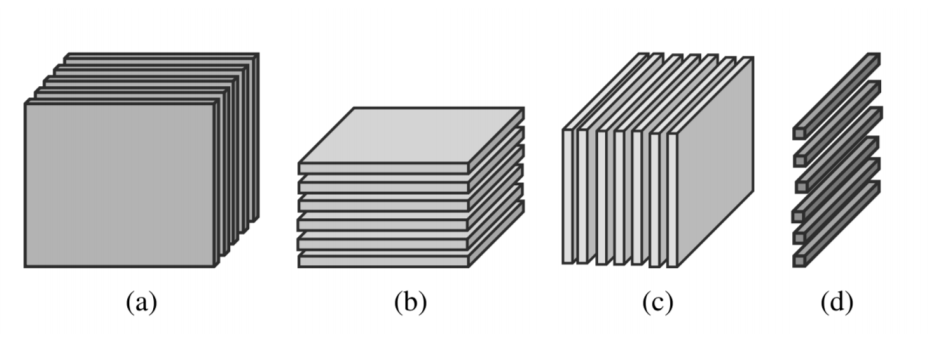
Fig. 1: (a) Frontal, (b) horizontal, and (c) lateral slices of a third order tensor. (d) A mode-3 tube fibers.

2.1 Discrete Fourier Transformation

In this subsection we recall some definitions and properties of the discrete Fourier transformation and the T-product. The Discrete Fourier Transformation (DFT) plays a very important role in the definition of the T-product of tensors. The DFT on a vector $v\in{\mathcal{R}}^{n}$ is defined by

$$\tilde{v}=F_{n}(v)\in{\mathbb{C}}^{n},$$ (4)

where $F_{n}$ is the matrix defined as

$$F_{n}(v)=\left(\begin{array}[]{ccccc}1&1&1&\ldots&1\\ 1&\omega&\omega^{2}&\ldots&\omega^{n-1}\\ \vdots&\vdots&\vdots&\ldots&\vdots\\ 1&\omega^{n-1}&\omega^{2(n-1)}&\ldots&\omega^{(n-1)(n-1)}\\ \end{array}\right)\in{\mathbb{C}}^{n\times n},$$ (5)

where $\omega=e^{\frac{-2\pi i}{n}}$ with $i^{2}=-1$. It is not difficult to show that (see [13])

$$F_{n}^{*}=\overline{F}_{n},\;{\rm and}\;F_{n}^{*}F_{n}=F_{n}F_{n}^{*}=nI_{n}.$$ (6)

Then $F_{n}^{-1}=\displaystyle\frac{1}{n}\overline{F}_{n}$ which show that $\displaystyle\frac{1}{\sqrt{n}}F_{n}$ is a unitary matrix.
The cost of computing the vector $\tilde{v}$ directly from (4) is $O(n^{2})$. Using the Fast Fourier Transform (fft), it will costs $O(nlog(n))$. It is known that

$$F_{n}\,{\rm circ}(v)\,F_{n}^{-1}={\rm Diag}(\tilde{v}),\\$$ (7)

which is equivalent to

$$F_{n}\,{\rm circ}(v)\,F_{n}^{*}=n\,{\rm Diag}(\tilde{v}),\\$$ (8)

where

$${\rm circ}(v)=\left(\begin{array}[]{cccc}v_{1}&v_{2}&\ldots&v_{n}\\ v_{2}&v_{1}&\ldots&v_{3}\\ \vdots&\vdots&\ldots&\vdots\\ v_{n}&v_{n-1}&\ldots&v_{1}\\ \end{array}\right),$$

and ${\rm Diag}(\tilde{v}),$ is the diagonal matrix whose $i$-th diagonal element is ${\rm Diag}(\tilde{v})_{i}$. The decomposition (7) shows that the columns of $F_{n}$ are the eigenvectors of ${\rm circ}(v))^{T}$.

2.2 Definitions and properties of the T-product

In this part, we briefly review some concepts and notations, which play a central role for the elaboration of the global iterative methods based on T-product; see [3, 17, 26, 24] for more details. Let $\mathscr{A}\in\mathbb{R}^{n_{1}\times n_{2}\times n_{3}}$ be a third-order tensor, then the operations bcirc, unfold and fold are defined by

$${\tt bcirc}(\mathscr{A})=\left({\begin{array}[]{*{20}{c}}{{A_{1}}}&{{A_{{n_{3}}}}}&{{A_{{n_{3-1}}}}}&\ldots&{{A_{2}}}\\ {{A_{2}}}&{{A_{1}}}&{{A_{{n_{3}}}}}&\ldots&{{A_{3}}}\\ \vdots&\ddots&\ddots&\ddots&\vdots\\ {{A_{{n_{3}}}}}&{{A_{{n_{3-1}}}}}&\ddots&{{A_{2}}}&{{A_{1}}}\end{array}}\right)\in{\mathcal{R}}^{n_{1}n_{2}\times n_{2}n_{3}},$$

$${\tt unfold}(\mathscr{A})=\begin{pmatrix}A_{1}\\ A_{2}\\ \vdots\\ A_{n_{3}}\end{pmatrix}\in\mathbb{R}^{n_{2}n_{3}\times m_{2}},\qquad{\tt fold}({\tt unfold}(\mathscr{A}))=\mathscr{A}.$$

Let $\widetilde{\mathscr{A}}$ be the tensor obtained by applying the DFT on all the tubes of the tensor $\mathscr{A}$. With the Matlab command ${\tt fft}$, we have

$$\widetilde{\mathscr{A}}={\tt fft}(\mathscr{A},[],3),\;{\rm and}\;\;{\tt ifft}(\widetilde{\mathscr{A}},[],3)=\mathscr{A},$$

where ${\tt ifft}$ denotes the Inverse Fast Fourier Transform.
Let ${\bf A}$ be the matrix

$${\bf A}=\left(\begin{array}[]{cccc}{A}^{(1)}&&&\\ &{A}^{(2)}&&\\ &&\ddots&\\ &&&{A}^{(n_{3})}\\ \end{array}\right),$$ (9)

and the matrices ${A}^{(i)}$’s are the frontal slices of the tensor ${\widetilde{\mathscr{A}}}$.
The block circulant matrix ${\tt bcirc}(\mathscr{A})$ can also be block diagonalized by using the DFT and this gives

$$(F_{n_{3}}\otimes I_{n_{1}})\,{\tt bcirc}(\mathscr{A})\,(F_{n_{3}}^{-1}\otimes I_{n_{2}})={\bf A},$$ (10)

As noticed in [24, 30], the diagonal blocks of the matrix ${\bf A}$ satisfy the following property

$$\left\{\begin{array}[]{ll}{A}^{(1)}\in{\mathcal{R}}^{n_{1}\times n_{2}}\\ conj({A}^{(i)})=A^{(n_{3}-i+2)},\\ \end{array}\right.$$ (11)

where $conj({A}^{(i)})$ is the complex conjugate of the matrix ${A}^{(i)}$. Next we recall the definition of the T-product.

Definition 1.

The T-product ($\star$) between two tensors $\mathscr{A}\in\mathbb{R}^{n_{1}\times n_{2}\times n_{3}}$ and $\mathscr{B}\in\mathbb{R}^{n_{2}\times m\times n_{3}}$ is an ${n_{1}\times m\times n_{3}}$ tensor given by:

$$\mathscr{A}\star\mathscr{B}={\rm fold}({\rm bcirc}(\mathscr{A}){\rm unfold}(\mathscr{B})).$$

Notice that from the relation (9), we can show that the the product $\mathscr{C}=\mathscr{A}\star\mathscr{B}$ is equivalent to ${\bf C}={\bf A}\,{\bf B}$. So, the efficient way to compute the T-product is to use Fast Fourier Transform (FFT). Using the relation (11), the following algorithm allows us to compute in an efficient way the T-product of the tensors $\mathscr{A}$ and $\mathscr{B}$, see [30].

Algorithm 1 Computing the T-product via FFT

Inputs: $\mathscr{A}\in\mathbb{R}^{n_{1}\times n_{2}\times n_{3}}$ and $\mathscr{B}\in\mathbb{R}^{n_{2}\times m\times n_{3}}$
Output: $\mathscr{C}=\mathscr{A}\star\mathscr{B}\in\mathbb{R}^{n_{1}\times m\times n_{3}}$

1. Compute $\mathscr{\widetilde{A}}={\tt fft}(\mathscr{A},[],3)$ and $\mathscr{\widetilde{B}}={\tt fft}(\mathscr{B},[],3)$.

2. Compute each frontal slices of $\mathscr{\widetilde{C}}$ by
   

   $$C^{(i)}=\left\{\begin{array}[]{ll}A^{(i)}B^{(i)},\quad\quad\quad i=1,\ldots,\lfloor\displaystyle\frac{{n_{3}}+1}{2}\rfloor\\ conj({C}^{(n_{3}+i-2)}),\quad\quad i=\lfloor\displaystyle\frac{{n_{3}}+1}{2}\rfloor+1,\ldots,n_{3}.\\ \end{array}\right.$$

3. Compute $\mathscr{C}={\tt ifft}(\widetilde{C},[],3)$.

For the T-product, we have the following definitions

Definition 2.

The identity tensor $\mathscr{I}_{n_{1}n_{1}n_{3}}$ is the tensor whose first frontal slice is the identity matrix $I_{n_{1},n_{1}}$ and the other frontal slices are all zeros.

Definition 3.

1. An $n_{1}\times n_{1}\times n_{3}$ tensor $\mathscr{A}$ is invertible, if there exists a tensor $\mathscr{B}$ of order $n_{1}\times n_{1}\times n_{3}$ such that

   $$\mathscr{A}\star\mathscr{B}=\mathscr{I}_{n_{1}n_{1}n_{3}}\qquad\text{and}\qquad\mathscr{B}\star\mathscr{A}=\mathscr{I}_{n_{1}n_{1}n_{3}}.$$

   In that case, we set $\mathscr{B}=\mathscr{A}^{-1}$. It is clear that $\mathscr{A}$ is invertible if and only if ${\rm bcirc}(\mathscr{A})$ is invertible.

2. The transpose of $\mathscr{A}$ is obtained by transposing each of the frontal slices and then reversing the order of transposed frontal slices 2 through $n_{3}$.

3. If $\mathscr{A}$, $\mathscr{B}$ and $\mathscr{A}$ are tensors of appropriate order, then

   $$(\mathscr{A}\star\mathscr{B})\star\mathscr{C}=\mathscr{A}\star(\mathscr{B}\star\mathscr{C}).$$

4. Suppose $\mathscr{A}$ and $\mathscr{B}$ are two tensors such $\mathscr{A}\star\mathscr{B}$ and $\mathscr{B}^{T}\star\mathscr{A}^{T}$ are defined. Then

   $$(\mathscr{A}\star\mathscr{B})^{T}=\mathscr{B}^{T}\star\mathscr{A}^{T}.$$

Exemple 1.

If $\mathscr{A}\in\mathbb{R}^{n_{1}\times n_{2}\times 5}$ and its frontal slices are given by the $n_{1}\times n_{2}$ matrices $A_{1},A_{2},A_{3},A_{4},A_{5}$, then

$$\mathscr{A}^{T}={\tt fold}\begin{pmatrix}A_{1}^{T}\\ A_{5}^{T}\\ A_{4}^{T}\\ A_{3}^{T}\\ A_{2}^{T}\\ \end{pmatrix}.$$

Definition 4.

Let $\mathscr{A}$ and $\mathscr{B}$ two tensors in $\mathbb{R}^{n_{1}\times n_{2}\times n_{3}}$. Then

1. The scalar inner product is defined by

   $$\langle\mathscr{A},\mathscr{B}\rangle=\displaystyle\sum_{i_{1}=1}^{n_{1}}\sum_{i_{2}=1}^{n_{2}}\sum_{i_{3}=1}^{n_{3}}a_{i_{1}i_{2}i_{3}}b_{i_{1}i_{2}i_{3}}.$$

2. The norm of $\mathscr{A}$ is defined by

   $$\|\mathscr{A}\|_{F}=\displaystyle\sqrt{\langle\mathscr{A},\mathscr{A}\rangle}.$$

Remark 2.1.

Another interesting way for computing the scalar product and the associated norm is as follows:

$$\langle\mathscr{A},\mathscr{B}\rangle=\displaystyle\frac{1}{n_{3}}\langle{\bf A},{\bf B}\rangle;\;\;\|\mathscr{A}\|_{F}=\displaystyle\frac{1}{\sqrt{n_{3}}}\|{{\bf A}}\|_{F},$$

where the block diagonal matrix ${\bf A}$ is defined by (9).

Definition 5.

An $n_{1}\times n_{1}\times n_{3}$ tensor $\mathscr{Q}$ is orthogonal if

$$\mathscr{Q}^{T}\star\mathscr{Q}=\mathscr{Q}\star\mathscr{Q}^{T}=\mathscr{I}_{n_{1}n_{1}n_{3}}.$$

Lemma 6.

If $\mathscr{Q}$ is an orthogonal tensor, then

$$\left\|\mathscr{Q}\star\mathscr{A}\right\|_{F}=\left\|\mathscr{A}\right\|_{F}.$$

Definition 7.

[24] A tensor is called f-diagonal if its frontal slices are orthogonal matrices. It is called upper triangular if all its frontal slices are upper triangular.

Definition 8.

[34](Block tensor based on T-product) Suppose $\mathscr{A}\in{\mathbb{R}}^{n_{1}\times m_{1}\times n_{3}}$, $\mathscr{B}\in{\mathbb{R}}^{n_{1}\times m_{2}\times n_{3}}$, $\mathscr{C}\in{\mathbb{R}}^{n_{2}\times m_{1}\times n_{3}}$ and $\mathscr{D}\in{\mathbb{R}}^{n_{2}\times m_{2}\times n_{3}}$ are four tensors. The block tensor

$$\left[{\begin{array}[]{*{20}{c}}{\mathscr{A}}&{\mathscr{B}}\\ {\mathscr{C}}&{\mathscr{D}}\\ \end{array}}\right]\in{\mathbb{R}}^{(n_{1}+n_{2})\times(m_{1}+m_{2})\times n_{3}}$$

is defined by compositing the frontal slices of the four tensors.

Now we introduce the T-diamond tensor product.

Definition 9.

Let $\mathscr{A}=[\mathscr{A}_{1},\ldots,\mathscr{A}_{p}]\in{\mathbb{R}}^{n_{1}\times ps\times n_{3}},$ where $\mathscr{A}_{i}\;n_{1}\times s\times n_{3},\,i=1,...,p$ and let $\mathscr{B}=[\mathscr{B}_{1},\ldots,\mathscr{B}_{l}]\in{\mathbb{R}}^{n_{1}\times\ell s\times n_{3}}$ with $\mathscr{B}_{j};n_{1}\times s\times n_{3},\,j=1,...\ell$. Then, the product $\mathscr{A}^{T}\diamondsuit\mathcal{B}$ is the size matrix $p\times\ell$ given by :

$$(\mathscr{A}^{T}\diamondsuit\mathcal{B})_{i,j}=\langle\mathscr{A}_{i},\mathscr{B}_{j}\rangle\;\;.$$

3 Global tensor T-Arnoldi and global tensor T-Golub-Kahan

3.1 The tensor T-global GMRES

Consider now the following tensor linear system of equations

$$\mathscr{A}\star\mathscr{X}=\mathscr{C},$$ (12)

where $\mathscr{A}\in\mathbb{R}^{n\times n\times p}$, $\mathscr{C}$ and $\mathscr{X}\in\mathbb{R}^{n\times s\times p}$.
We introduce the tensor Krylov subspace $\mathcal{\mathscr{TK}}_{m}(\mathscr{A},\mathscr{V})$ associated to the T-product, defined for the pair $(\mathscr{A},\mathscr{V})$ as follows

$$\mathcal{\mathscr{TK}}_{m}(\mathscr{A},\mathscr{V})={\rm Tspan}\{\mathscr{V},\mathscr{A}\star\mathscr{V},\ldots,\mathscr{A}^{m-1}\star\mathscr{V}\}\\ =\left\{\mathscr{Z}\in\mathbb{R}^{n\times s\times n_{3}},\mathscr{Z}=\sum_{i=1}^{m}\alpha_{i}\left(\mathscr{A}^{i-1}\star\mathscr{V}\right)\right\}$$ (13)

where $\alpha_{i}\in\mathbb{R}$, $\mathscr{A}^{i-1}\star\mathscr{V}=\mathscr{A}^{i-2}\star\mathscr{A}\star\mathscr{V}$, for $i=2,\ldots,m$ and $\mathscr{A}^{0}$ is the identity tensor. We can now give a new version of the Tensor T-global Arnoldi algorithm.

Algorithm 2 Tensor T-global Arnoldi

1. Input. $\mathscr{A}\in\mathbb{R}^{n\times n\times p}$, $\mathscr{V}\in\mathbb{R}^{n\times s\times p}$ and and the positive integer $m$.

2. Set $\beta=\|\mathscr{V}\|_{F}$, $\mathscr{V}_{1}=\dfrac{\mathscr{V}}{\beta}$

3. For $j=1,\ldots,m$

   1. $\mathscr{W}=\mathscr{A}\star\mathscr{V}_{j}$

   2. for $i=1,\ldots,j$

      1. $h_{i,j}=\langle\mathscr{V}_{i},\mathscr{W}\rangle$

      2. $\mathscr{W}=\mathscr{W}-h_{i,j}\;\mathscr{V}_{i}$

   3. End for

   4. $h_{j+1,j}=\|\mathscr{W}\|_{F}$. If $h_{j+1,j}=0$, stop; else

   5. $\mathcal{V}_{j+1}=\mathscr{W}/h_{j+1,j}$.

4. End

Proposition 10.

Assume that m steps of Algorithm (2) have been run. Then, the tensors $\mathscr{V}_{1},\ldots,\mathscr{V}_{m}$, form an orthonormal basis of the tensor global Krylov subspace $\mathscr{TK}^{g}_{m}(\mathscr{A},\mathscr{V})$.

Proof.

This can be shown easily by induction on $m$. ∎

Let $\mathbb{V}_{m}$ be the $(n\times(sm)\times p)$ tensor with frontal slices $\mathscr{V}_{1},\ldots,\mathscr{V}_{m}$ and let ${\widetilde{H}}_{m}$ be the $(m+1)\times m$ upper Hesenberg matrix whose elements are the $h_{i,j}$’s defined by Algorithm 2. Let ${H}_{m}$ be the matrix obtained from $\widetilde{{H}}_{m}$ by deleting its last row; $H_{.,j}$ will denote the $j$-th column of the matrix $H_{m}$ and $\mathscr{A}\star\mathbb{V}_{m}$ is the $(n\times(sm)\times p)$ tensor with frontal slices $\mathscr{A}\star\mathscr{V}_{1},\ldots,\mathscr{A}\star\mathscr{V}_{m}$ respectively given by

$$\mathbb{V}_{m}:=\left[\mathscr{V}_{1},\ldots,\mathscr{V}_{m}\right],\;\;\;{\rm and}\;\;\;\mathscr{A}\star\mathbb{V}_{m}:=[\mathscr{A}\star\mathscr{V}_{1},\ldots,\mathscr{A}\star\mathscr{V}_{m}].$$ (14)

We introduce the product $\circledast$ defined by:

$$\mathbb{V}_{m}\circledast y=\sum_{j=1}^{m}{y}_{j}\mathscr{{V}}_{j},\;y=(y_{1},\ldots,y_{m})^{T}\in\mathbb{R}^{m}.$$

We set the following notation:

$$\mathbb{V}_{m}\circledast{{{H}}_{m}}=\left[\mathbb{V}_{m}\circledast H_{.,1},\ldots,\mathscr{V}_{m}\circledast H_{.,m}\right].$$

Then, it is easy to see that $\forall$ $u\,\text{and}\,v$ $\in\mathbb{R}^{m}$, we have

$$\mathbb{V}_{m}\circledast(u+v)=\mathbb{V}_{m}\circledast u+\mathbb{V}_{m}\circledast v\quad\text{and}\quad(\mathbb{V}_{m}\circledast H_{m})\circledast u=\mathbb{V}_{m}\circledast(H_{m}\;u).$$ (15)

With these notations, we can show the following result (proposition) that will be useful later on.

Proposition 11.

Let $\mathbb{V}_{m}$ be the tensor defined by $\left[\mathscr{V}_{1},\ldots,\mathscr{V}_{m}\right]$ where $\mathscr{V}_{i}\in\mathbb{R}^{n\times s\times p}$ are defined by the Tensor T-global Arnoldi algorithm. Then, we have

$$\|\mathbb{V}_{m}\circledast y\|_{F}=\|y\|_{2},\;\forall y=(y_{1},\ldots,y_{m})^{T}\in\mathbb{R}^{m}.$$ (16)

Proof.

From the definition of the product $\circledast$, we have $\sum_{j=1}^{m}{y}_{j}\mathscr{{V}}_{j}=\mathbb{V}_{m}\circledast y$. Therefore,

$$\|\mathbb{V}_{m}\circledast y\|_{F}^{2}=\left<\sum_{j=1}^{m}{y}_{j}\mathscr{{V}}_{j},\sum_{j=1}^{m}{y}_{j}\mathscr{{V}}_{j}\right>_{F}.$$

But, since the tensors $\mathscr{{V}}_{i}$’s are orthonormal, it follows that

$$\|\mathbb{V}_{m}\circledast y\|_{F}^{2}=\sum_{j=1}^{m}{y}_{j}^{2}={\|y\|_{2}^{2}},$$

which shows the result.

∎

With the above notations, we can easily prove the results of the following proposition :

Proposition 12.

Suppose that m steps of Algorithm 2 have been run. Then, the following statements hold:

$$\mathscr{A}\star\mathbb{V}_{m} = \mathbb{V}_{m}\circledast{{{H}}_{m}}+h_{m+1,m}\left[\mathscr{O}_{n\times s\times p},\ldots,\mathscr{O}_{n\times s\times p},\mathscr{V}_{m+1}\right],$$ (17)

$$\mathscr{A}\star\mathbb{V}_{m} = \mathbb{V}_{m+1}\circledast\widetilde{{H}}_{m},$$ (18)

$$\mathbb{V}_{m}^{T}\diamondsuit\mathscr{A}\star\mathbb{V}_{m} = {H}_{m},$$ (19)

$$\mathbb{V}_{m+1}^{T}\diamondsuit\mathscr{A}\star\mathbb{V}_{m} = \widetilde{{H}}_{m},$$ (20)

$$\mathbb{V}_{m}^{T}\diamondsuit\mathbb{V}_{m} = {I}_{m},$$ (21)

where ${I}_{m}$ the identity matrix and $\mathscr{O}$ is the tensor having all its entries equal to zero.

Proof.

From Algorithm 2, we have $\mathscr{A}\star\mathscr{V}_{j}=\sum_{i=1}^{j+1}h_{i,j}\mathscr{V}_{i}$. Using the fact that $\mathscr{A}\star\mathbb{V}_{m}=\left[\mathscr{A}\star\mathscr{V}_{1},\ldots,\mathscr{A}\star\mathscr{V}_{m}\right]$, the $j$-th frontal slice of $\mathscr{A}\star\mathbb{V}_{m}$ is given by

$$(\mathscr{A}\star\mathbb{V}_{m})_{j}=\mathscr{A}\star\mathscr{V}_{j} =\sum_{i=1}^{j+1}h_{i,j}\mathscr{V}_{i}.$$

Furthermore, from the definition of the $\circledast$ product, we have

$$(\mathbb{V}_{m+1}\circledast\widetilde{{H}}_{m})_{j} =\mathbb{V}_{m+1}\circledast H_{.,j},$$

$$=\sum_{i=1}^{j+1}h_{i,j}\mathscr{V}_{i},$$

which proves the first two relations. The other relations follow from the definition of T-diamond product ∎

In the sequel, we develop the tensor T-global GMRES algorithm for solving the problem (12). It could be considered as generalization of the well known global GMERS algorithm [19]. Let $\mathscr{{X}}_{0}\in\mathbb{R}^{n\times s\times p}$ be an arbitrary initial guess with the corresponding residual $\mathscr{R}_{0}=\mathscr{C}-\mathscr{A}\star\mathscr{X}_{0}$. The aim of tensor T-global GMRES method is to find and approximate solution $\mathscr{X}_{m}$ approximating the exact solution $\mathscr{X}^{*}$ of (12) such that

$$\mathscr{X}_{m}-\mathscr{X}_{0}\in\mathscr{TK}^{g}_{m}(\mathscr{A},\mathscr{R}_{0}),$$ (22)

with the classical minimization property

$$\|\mathscr{R}_{m}\|_{F}=\displaystyle\min_{\mathscr{X}\in\mathscr{X}_{0}+\mathscr{TK}^{g}_{m}(\mathscr{A},\mathscr{R}_{0})}\left\{\|\mathscr{C}-\mathscr{A}\star\mathscr{X}\|_{F}\right\}.$$ (23)

Let $\mathscr{X}_{m}=\mathscr{X}_{0}+\mathbb{V}_{m}\circledast y$ with ${y}\in\mathbb{R}^{m}$, be the approximate solution satisfying (22). Then,

$$\mathscr{R}_{m}= \mathscr{C}-\mathscr{A}\star\mathscr{X}_{m},$$

$$= \mathscr{C}-\mathscr{A}\star\left(\mathscr{X}_{0}+\mathbb{V}_{m}\circledast y\right),$$

$$= \mathscr{C}-\mathscr{A}\star\mathscr{X}_{0}-\mathscr{A}\star(\mathbb{V}_{m}\circledast y),$$

$$= \mathscr{R}_{0}-\left(\mathscr{A}\star\mathbb{V}_{m}\right)\circledast y.$$

It follows then that

$$\|\mathscr{R}_{m}\|_{F} =\displaystyle\min_{y\in\mathbb{R}^{m}}\|\mathscr{R}_{0}-(\mathscr{A}\star\mathbb{V}_{m})\circledast y\|_{F},$$

where $\mathscr{A}\star\mathbb{V}_{m}:=[\mathscr{A}\star\mathscr{V}_{1},\ldots,\mathscr{A}\star\mathscr{V}_{m}]$ is the $(n\times sm\times p)$ tensor defined earlier.
Using Propositions 11 and the fact that $\mathscr{R}_{0}=\|\mathscr{R}_{0}\|_{F}\mathscr{V}_{1}$ with $\mathscr{V}_{1}=\mathscr{V}_{m+1}\circledast e_{1}$, where $e_{1}$ the first canonical basis vector in $\mathbb{R}^{m+1}$, we get

$$\|\mathscr{R}_{0}-(\mathscr{A}\star\mathbb{V}_{m})\circledast y\|_{F} =\|\mathscr{R}_{0}-(\mathbb{V}_{m+1}\circledast\widetilde{{H}}_{m})\circledast y\|_{F},$$

$$=\|\|\mathscr{R}_{0}\|_{F}(\mathbb{V}_{m+1}\circledast e_{1})-(\mathbb{V}_{m+1}\circledast\widetilde{{H}}_{m})\circledast y\|_{F},$$

$$=\|\mathbb{V}_{m+1}\circledast(||\mathscr{R}_{0}\|_{F}e_{1}-\widetilde{{H}}_{m}y)\|_{F},$$

$$=\|\;\|\mathscr{R}_{0}\|_{F}\;e_{1}-\widetilde{{H}}_{m}y\|_{2}.$$

Finally, we obtain

$$\mathscr{X}_{m}=\mathscr{X}_{0}+\mathbb{V}_{m}\circledast y,$$ (24)

where,

$$y=\text{arg }\min_{{{y}}\in\mathbb{R}^{m}}||\;||\mathscr{R}_{0}||_{F}\;e_{1}-\widetilde{{H}}_{m}y)||_{2}.$$ (25)

3.2 Tensor T-global Golub Kahan algorithm

Instead of using the tensor T-global Arnoldi to generate a basis for the projection subspace, we can define T-version of the tensor global Lanczos process. Here, we will use the tensor Golub Kahan algorithm related to the T-product. We notice here that we already defined in [12] another version of the tensor Golub Kahan algorithm by using the $m$-mode or the Einstein products with applications to color image restoration.
Let $\mathscr{A}\in\mathbb{R}^{n\times\ell\times p}$ be a tensor and let $\mathscr{U}\in\mathbb{R}^{\ell\times s\times p}$ and $\mathscr{V}\in\mathbb{R}^{n\times s\times p}$ two other tensors. Then, the Tensor T-global Golub Kahan bidiagonalization algorithm (associated to the T-product) is defined as follows

Algorithm 3 The Tensor T-global Golub Kahan algorithm

1. Input. The tensors $\mathscr{A}$, $\mathscr{V}$, and $\mathscr{U}$ and an integer $m$.

2. Set $\beta_{1}=\|\mathscr{V}\|_{F}$, $\alpha_{1}=\|\mathscr{U}\|_{F}$, $\mathscr{V}_{1}=\mathscr{V}/\beta_{1}$ and $\mathscr{U}_{1}=\mathscr{U}/\alpha_{1}$.

3. for $j=2,\ldots,m$

   1. $\widetilde{\mathscr{V}}=\mathscr{A}\star\mathscr{U}_{j-1}-\alpha_{j-1}\mathscr{V}_{j-1}$

   2. $\beta_{j}=\|\widetilde{\mathscr{V}}\|_{F}$ if $\beta_{j}=0$ stop, else

   3. $\mathscr{V}_{j}=\widetilde{\mathscr{V}}/\beta_{j}$

   4. $\widetilde{\mathscr{U}}=\mathscr{A}^{T}\star\mathscr{V}_{j}-\beta_{j}\mathscr{U}_{j-1}$

   5. $\alpha_{j}=\|\widetilde{\mathscr{U}}\|_{F}$

   6. if $\alpha_{j}=0$ stop, else

   7. $\mathscr{U}_{j}=\widetilde{\mathscr{U}}/\alpha_{j}$

Let $\widetilde{C}_{m}$ be the upper bidiagonal $((m+1)\times m)$ matrix

$$\widetilde{{{C}}}_{m}=\left[\begin{array}[]{*{20}{c}}{{{\alpha}_{1}}}&{{}}\hfil&&\\ {\beta}_{2}&{{{\alpha}_{2}}}&\ddots&\\ &\ddots&\ddots&\\ &&{\beta}_{m}&{\alpha}_{m}\\ &&&{\beta}_{m+1}\end{array}\right]$$

and let ${{{C}}}_{m}$ be the $(m\times m)$ matrix obtain by deleting the last row of $\widetilde{{{C}}}_{m}$. We denote by $C_{.,j}$ will denote the $j$-th column of the matrix $C_{m}$. Let $\mathbb{U}_{m}$ and $\mathscr{A}\star\mathbb{U}_{m}$ be the $(\ell\times(sm)\times p)$ and $(n\times(sm)\times p)$ tensors with frontal slices $\mathscr{U}_{1},\ldots,\mathscr{U}_{m}$ and $\mathscr{A}\star\mathscr{U}_{1},\ldots,\mathscr{A}\star\mathscr{U}_{m}$, respectively, and let $\mathbb{V}_{m}$ and $\mathscr{A}^{T}\star\mathbb{V}_{m}$ be the $(n\times(sm)\times p)$ and $(\ell\times(sm)\times p)$ tensors with frontal slices $\mathscr{V}_{1},\ldots,\mathscr{V}_{m}$ and $\mathscr{A}^{T}\star\mathscr{V}_{1},\ldots,\mathscr{A}^{T}\star\mathscr{V}_{m}$, respectively. We set

$$\mathbb{U}_{m}: =\left[\mathscr{U}_{1},\ldots,\mathscr{U}_{m}\right],\;\;\;{\rm and}\;\;\;\mathscr{A}\star\mathbb{U}_{m}:=[\mathscr{A}\star\mathscr{U}_{1},\ldots,\mathscr{A}\star\mathscr{U}_{m}],$$ (26)

$$\mathbb{V}_{m}: =\left[\mathscr{V}_{1},\ldots,\mathscr{V}_{m}\right],\;\;\;{\rm and}\;\;\;\mathscr{A}^{T}\star\mathbb{V}_{m}:=[\mathscr{A}^{T}\star\mathscr{V}_{1},\ldots,\mathscr{A}^{T}\star\mathscr{V}_{m}].$$ (27)

Then, the following proposition can be established

Proposition 13.

The tensors produced by the tensor T-global Golub-Kahan algorithm satisfy the following relations

$$\mathcal{A}\star\mathbb{U}_{m} = \mathbb{V}_{m+1}\circledast{\widetilde{{{C}}}}_{m},$$ (28)

$$= \mathbb{V}_{m}\circledast{{{{C}}}}_{m}+{\beta}_{m+1}\left[\mathscr{O}_{n\times s\times p},\ldots,\mathscr{O}_{n\times s\times p},\mathscr{V}_{m+1}\right],$$ (29)

$$\mathscr{A}^{T}\star\mathbb{V}_{m} = \mathbb{U}_{m}\circledast{\widetilde{{{C}}}}_{m}^{T}.$$ (30)

Proof.

Using $\mathscr{A}\star\mathbb{U}_{m}=[\mathscr{A}\star\mathscr{U}_{1},\ldots,\mathscr{A}\star\mathscr{U}_{m}]\in\mathbb{R}^{n\times(sm)\times n_{3}}$ , the ($j-1$)-th lateral slice of $(\mathscr{A}\star\mathbb{U}_{m})$ is given by

$$(\mathcal{A}\star\mathbb{U}_{m})_{j-1}=\mathscr{A}\star\mathscr{U}_{j-1}={\alpha}_{j-1}\mathscr{V}_{j-1}+{\beta}_{j}\mathcal{V}_{j}.$$

Furthermore, from the definition of the $\circledast$ product, we have

$$(\mathbb{V}_{m+1}\circledast\widetilde{{C}}_{m})_{j-1} =\mathbb{V}_{m+1}\circledast C_{.,j-1},$$

$$=\sum_{i=1}^{j+1}c_{i,j-1}\mathscr{V}_{i},$$

$$={\alpha}_{j-1}\mathscr{V}_{j-1}+{\beta}_{j}\mathcal{V}_{j}$$

and for $j=m$, $\mathbb{U}_{m}\circledast\mathscr{C}_{.,m}=\mathscr{A}\star\mathscr{U}_{m}+{\beta}_{m+1}\mathscr{V}_{m+1}$ and the result follows.
To derive (4.5) , one may first notice that from Algorithm 3, we have

$$(\mathcal{A}^{T}\star\mathbb{V}_{m})_{j}=\mathscr{A}^{T}\star\mathscr{V}_{j}={\alpha}_{j}\mathscr{U}_{j}+{\beta}_{j}\mathcal{U}_{j-1}.$$

Considering now the $j$-th frontal slice of the right-hand side of (4.5), the assertion can be easily deduced . ∎

Proposition 14.

Let $\mathscr{{X}}_{m}=\mathscr{{X}}_{0}+\mathbb{U}_{m}\circledast y\in\mathbb{R}^{\ell\times s\times p}$ with ${{y}}\in\mathbb{R}^{m},$ where $\mathbb{U}_{m}$ is obtained from Algorithm 3, be an approximation of (12). Then, we have

$$\|\mathscr{C}-\mathscr{A}\star\mathscr{X}_{m}\|_{F}=\|\beta_{1}e_{1}-{\widetilde{C}}_{m}y\|_{2},$$ (31)

where $\beta_{1}=\|\mathscr{C}\|_{F}$.

Proof.

Using representation (28) and the fact that $\mathscr{C}=\mathbb{V}_{m+1}\circledast(\beta_{1}e_{1})$ with $\beta_{1}=\|\mathscr{C}\|_{F}$, we get

$$\|\mathscr{C}-\mathscr{A}\star\mathscr{X}_{m}\|_{F} =\|\mathbb{V}_{m+1}\circledast(\beta_{1}e_{1})-(\mathbb{V}_{m+1}\circledast{\widetilde{C}}_{m})\circledast y|\|_{F},$$

$$=|||\mathbb{V}_{m+1}\circledast(\beta_{1}e_{1}-{\widetilde{C}}_{m}y)||_{F},$$

$$=||\beta_{1}e_{1}-{\widetilde{C}}_{m}y||_{2}.$$

∎

4 Application to discrete-ill posed tensor problems

We consider the following discrete ill-posed tensor equation

$$\mathscr{A}\star\mathscr{X}=\mathscr{C},\quad\mathscr{C}=\widehat{\mathscr{C}}+\mathscr{N},$$ (32)

where $\mathscr{A}\in{\mathcal{R}}^{n\times n\times s}$, $\mathscr{X}$, $\mathscr{N}$ (additive noise) and $\mathscr{C}$ are tensors in ${\mathcal{R}}^{n\times s\times p}$.
In color image processing, $p=3$, $\mathscr{A}$ represents the blurring tensor, $\mathscr{C}$ the blurry and noisy observed image, $\mathscr{X}$ is the image that we would like to restore and $\mathscr{N}$ is an unknown additive noise. Therefore, to stabilize the recovered image, regularization techniques are needed. There are several techniques to regularize the linear inverse problem given by equation (32); for the matrix case, see for example, [1, 9, 14, 15]. All of these techniques stabilize the restoration process by adding a regularization term, depending on some priori knowledge of the unknown image. One of the most regularization method is due to Tikhonov and is given as follows

$$\underset{\mathscr{X}}{\text{min}}\{\|\mathscr{A}\star\mathscr{X}-\mathscr{C}\|_{F}^{2}+\mu\|\mathscr{X}\|_{F}^{2}\}.$$ (33)

As problem (32) is large, Tikhonov regularization (33) may be very expensive to solve. One possibility is instead of regularizing the original problem, we apply the Tikhonov technique to the projected problem (25) which leads to the following problem

$$y_{m,\mu} = \arg\min_{y\in\mathbb{R}^{m}}\left(\|\mathscr{R}_{0}\|e_{1}-\widetilde{{H}}_{m}y\|_{2}+\mu\|y\|_{2}\right),$$ (34)

$$= \arg\min_{y\in\mathbb{R}^{m}}\left\|\left(\begin{array}[]{ll}\widetilde{H}_{m}\\ \mu I_{m}\end{array}\right)y-\left(\begin{array}[]{ll}\beta e_{1}\\ 0\end{array}\right)\right\|_{2}.$$ (39)

The minimizer $y_{m,\mu}$ can also be computed as the solution of the following normal equations associated with (39)

$${}\widetilde{H}_{m,\mu}y=\widetilde{H}_{m}^{T},\quad\widetilde{H}_{m,\mu}=(\widetilde{H}_{m}^{T}\widetilde{H}_{m}+\mu^{2}I_{m}).$$ (40)

Note that since the Tikhonov problem (40) is now a matrix one with small dimension as $m$ is generally small, the vector $y_{m,\mu}$, can thereby be inexpensively computed by some techniques such as the GCV method [14] or the L-curve criterion [15, 16, 11, 9]. To choose the regularization parameter, we can use the generalized cross-validation (GCV) method [14, 39]. Now for the GCV method, the regularization parameter is chosen by minimizing the following function

$$GCV(\mu)=\frac{\|\widetilde{H}_{m}y_{m,\mu}-{\bf\beta e_{1}}\|_{2}^{2}}{[tr(I_{m}-\widetilde{H}_{m}\widetilde{H}_{m,\mu}^{-1}\widetilde{H}_{m}^{T})]^{2}}=\frac{\|(I_{m}-\widetilde{H}_{m}\widetilde{H}_{m,\mu}^{-1}\widetilde{H}_{m}^{T}){\beta e_{1}}\|_{2}^{2}}{[tr(I_{m}-H_{m}H_{m,\mu}^{-1}\widetilde{H}_{m}^{T})]^{2}}.$$ (41)

To minimize (41), we take advantage of the the SVD decomposition of the low dimensional matrix $\widetilde{H}_{m}$ to obtain a more simple and computable expression of $GCV(\mu)$. Consider the SVD decomposition of $\widetilde{H}_{m}=U\Sigma V^{T}$. Then, the GCV is now expressed as (see [39])

$$GCV(\mu)=\frac{\displaystyle\sum_{i=1}^{m}\left(\frac{\widetilde{g}_{i}}{\sigma_{i}^{2}+\mu^{2}}\right)^{2}}{\displaystyle\left(\sum_{i=1}^{m}\frac{1}{\sigma_{i}^{2}+\mu^{2}}\right)^{2}},$$ (42)

where $\sigma_{i}$ is the $i$th singular value of the matrix $\widetilde{H}_{m}$ and $\widetilde{g}=\beta_{1}U^{T}e_{1}$.

In terms of practical implementations, it’s more convenient to introduce a restarted version of the tensor Global GMRES. This strategy is essentially based on restarting the tensor T-global Arnoldi algorithm. Therefore, at each restart, the initial guess $\mathscr{X}_{0}$ and the regularization parameter $\mu$ are updated employing the last values computed when the the number of inner iterations required is fulfilled. We note that as the number outer iterations increases it is possible to compute the $m$th residual without having to compute extra T-products. This is described in the following proposition.

Proposition 15.

At step $m$, the residual $\mathscr{R}_{m}=\mathscr{C}-\mathscr{A}\ast\mathscr{X}_{m}$ produced by the tensor Global GMRES method for tensor equation (1) has the following expression

$$\mathscr{R}_{m}=\mathbb{V}_{m+1}\circledast\left(\gamma_{m+1}Q_{m}e_{m+1}\right),$$ (43)

where $Q_{m}$ is the unitary matrix obtained from the QR decomposition of the upper Hessenberg matrix $\widetilde{H}_{m}$ and $\gamma_{m+1}$ is the last component of the vector $\left\|\mathscr{R}_{0}\right\|_{F}Q_{m}^{\mathrm{T}}e_{1}$ and $e_{m+1}=(0,0,\ldots,1)^{\mathrm{T}}\in\mathbb{R}^{m+1}.\\$ Furthermore,

$$\left\|\mathscr{R}_{m}\right\|_{F}=\left|\gamma_{m+1}\right|.$$ (44)

Proof.

At step $m$, the residual $\mathscr{R}_{m}$ can be expressed as

$$\mathscr{R}_{m}=\mathbb{V}_{m+1}\circledast\left(\beta e_{1}-\widetilde{H}_{m}y_{m}\right),$$

by considering the QR decomposition $\widetilde{H}_{m}=Q_{m}\widetilde{U}_{m}$ of the $(m+1)\times m$ matrix $\widetilde{H}_{m}$, we get

$$\mathscr{R}_{m}=\left(\mathbb{V}_{m+1}\circledast Q_{m}\right)\circledast\left(\beta Q_{m}^{T}e_{1}-\widetilde{U}_{m}y_{m}\right).$$

Since $y$ solves problem (25), it follows that

$$\mathscr{R}_{m}=\mathbb{V}_{m+1}\circledast\left(\gamma_{m+1}Q_{m}e_{m+1}\right),$$

where $\gamma_{m+1}$ is the last component of the vector $\beta Q_{m}^{T}e_{1}.$ Therefore,

$$\left\|\mathscr{R}_{m}\right\|_{F} = \left\|\mathbb{V}_{m+1}\circledast\left(\gamma_{m+1}Q_{m}e_{m+1}\right)\right\|_{F},$$

$$= \left\|\gamma_{m+1}Q_{m}e_{m+1}\right\|_{2},$$

$$= \left|\gamma_{m+1}\right|,$$

which shows the results. ∎

The tensor T-global GMRES method is summarized in the following algorithm

Algorithm 4 Implementation of Tensor T-global GMRES(m)

1. Input. $\mathscr{A}\in\mathbb{R}^{n\times n\times n_{3}}$, $\mathscr{V},\mathscr{B},\mathscr{X}_{0}\in\mathbb{R}^{n\times s\times n_{3}}$, the maximum number of iteration $\text{Iter}_{\text{max}}$ and a tolerance $tol>0$ .

2. Output. $\mathscr{X}_{m}\in\mathbb{R}^{n\times s\times n_{3}}$ approximate solution of the system (12).

3. $k=1,\ldots,\text{Iter}_{\text{max}}$

   1. Compute $\mathscr{R}_{0}=\mathscr{C}-\mathscr{A}\star\mathscr{X}_{0}$.

   2. Apply Algorithm 2 to compute $\mathbb{V}_{m}$ and ${\widetilde{H}}_{m}$ .

   3. Determine $\mu_{k}$ as the parameter minimizing the GCV function given by (42)

   4. Compute the regularized solution $y_{m_{k},\mu}$ of the problem (39).

   5. Compute the approximate solution $\mathscr{X}_{m}=\mathscr{X}_{0}+\mathbb{V}_{m}\circledast y_{m,\mu_{k}}$

4. If $\|\mathscr{R}_{m}\|_{F}<tol$, stop, else

5. Set $\mathscr{X}_{0}=\mathscr{X}_{m}$ and go to 3-a.

6. End

We turn now to the tensor T-global Golub Kahan approach for the solving the Tikhonov regularization of the problem (1). Here, we apply the following Tikhonov regularization approach and solve the new problem

$$\underset{\mathscr{X}}{\text{min}}\{\|\mathscr{A}\star\mathscr{X}-\mathscr{C}\|_{F}^{2}+\mu^{-1}\|\mathscr{X}\|_{F}^{2}\}.$$ (45)

The use of $\mu^{-1}$ in (45) instead of $\mu$ will be justified below. In the what follows, we briefly review the discrepancy principle approach to determine a suitable regularization parameter, given an approximation of the norm of the additive error. We then assume that a bound $\varepsilon$ for $\|\mathscr{N}\|_{F}$ is available. This priori information suggests that $\mu$ has to be determined as soon as

$$\phi(\mu)\leq\eta\epsilon,$$ (46)

where $\phi(\mu)=\|\mathscr{A}\star\mathscr{X}-\mathscr{C}\|_{F}^{2}$ and $\eta\gtrapprox 1$ is refereed to as the safety factor for the discrepancy principle. A zero-finding method can be used to solve (46) in order to find a suitable regularization parameter which also implies that $\phi(\mu)$ has to be evaluated for several $\mu$-values. When the tensor $\mathscr{A}$ is of moderate size, the quantity $\phi(\mu)$ can be easily evaluated. This evaluation becomes expensive when the matrix $\mathscr{A}$ is large, which means that its evaluation by a zero-finding method can be very difficult and computationally expensive. We will approximate $\phi$ to be able to determine an estimate of $\|\mathscr{A}\star\mathscr{X}-\mathscr{C}\|_{F}^{2}$. Our approximation is obtained by using T-global Golub-Kahan bidiagonalization (T-GGKB) and Gauss-type quadrature rules. This connection provides approximations of moderate sizes to the quantity $\phi$, and therefore gives a solution method to inexpensively solve (46) by evaluating these small quantities that can successfully and inexpensively be employed to compute $\mu$ as well as defining a stopping criterion for the T-GGKB iterations; see [1, 2] for discussion on this method.
Introduce the functions (of $\mu$)

$$\mathcal{G}_{m}f_{\mu} = \|\mathscr{C}\|_{F}^{2}e_{1}^{T}(\mu C_{m}C_{m}^{T}+I_{m})^{-2}e_{1},$$ (47)

$${\mathcal{R}}_{m+1}f_{\mu} = \|\mathcal{C}\|_{F}^{2}e_{1}^{T}(\mu\widetilde{C}_{m}\widetilde{C}_{m}^{T}+I_{m+1})^{-2}e_{1};$$ (48)

The quantities $\mathcal{G}_{m}f$ and ${\mathcal{R}}_{m+1}f_{\mu}$ are refereed to as Gauss and Gauss-Radau quadrature rules, respectively, and can be obtained after $m$ steps of T-GGKB (Algorithm 3) applied to tensor $\mathscr{A}$ with initial tensor $\mathscr{C}$. These quantities approximate $\phi(\mu)$ as follows

$$\mathcal{G}_{m}f_{\mu}\leq\phi(\mu)\leq{\mathcal{R}}_{m+1}f_{\mu}.$$ (49)

Similarly to the approaches proposed in [1, 2], we therefore instead solve for $\mu$ the low dimensional nonlinear equation

$${\mathcal{G}}_{m}f_{\mu}=\epsilon^{2}.$$ (50)

We apply the Newton’s method to solve (50) that requires repeated evaluation of the function ${\mathcal{G}}_{m}f_{\mu}$ and its derivative, which are inexpensive computations for small $m$.
We now comment on the use of $\mu$ in (45) instead of $1/\mu,$ implies that the left-hand side of (46) is a decreasing convex function of $\mu.$ Therefore, there is a unique solution, denoted by $\mu_{\varepsilon},$ of

$$\phi(\mu)=\varepsilon^{2}$$

for almost all values of $\varepsilon>0$ of practical interest and therefore also of (50) for $m$ sufficiently large; see [1, 2] for analyses. We accept $\mu_{m}$ that solve (46) as an approximation of $\mu$, whenever we have

$${\mathcal{R}}_{m+1}f_{\mu}\leq\eta^{2}\epsilon^{2}.$$ (51)

If (51) does not hold for $\mu_{m}$, we carry out one more GGKB steps, replacing $m$ by $m+1$ and solve the nonlinear equation

$${\mathcal{G}}_{m+1}f_{\mu}=\epsilon^{2};$$ (52)

see [1, 2] for more details. Assume now that (51) holds for some $\mu_{m}$. The corresponding regularized solution is then computed by

$$\mathscr{X}_{m,\mu_{m}}=\mathbb{U}_{m}\circledast y_{m,\mu_{m}},$$ (53)

where $y_{m,\mu_{m}}$ solves

$$(\widetilde{C}_{m}^{T}\widetilde{C}_{m}+\mu_{m}^{-1}I_{m})y=\beta_{1}\widetilde{C}_{m}^{T}e_{1},\qquad\beta_{1}=\|\mathscr{C}\|_{F}.$$ (54)

It is also computed by solving the least-squares problem

$$\min_{y\in\mathbb{R}^{m}}\begin{Vmatrix}\begin{bmatrix}\mu_{m}^{1/2}\widetilde{C}_{m}\\ I_{m}\end{bmatrix}y-\beta_{1}\mu_{m}^{1/2}e_{1}\end{Vmatrix}_{2}.$$ (55)

The following result shows an important property of the approximate solution (53). We include a proof for completeness.

Proposition 16.

Let $\mu_{m}$ solve (50) and let $y_{m,\mu_{m}}$ solve (55). Then the associated approximate solution (53) of (45) satisfies

$$\left\|\mathscr{A}\ast\mathscr{X}_{m,\mu_{m}}-\mathscr{C}\right\|_{F}^{2}=R_{m+1}f_{\mu_{m}}.$$

Proof.

The representation of Proposition 13 show that

$$\mathscr{A}\ast\mathscr{X}_{m,\mu_{m}}=(\mathscr{A}\ast\mathbb{U}_{m})\circledast y_{m,\mu_{m}}=\mathbb{V}_{m+1}\circledast(\widetilde{C}_{m}y_{m,\mu_{m}}).$$

Using the above expression gives

$$\left\|\mathscr{A}\star\mathscr{X}_{m,\mu_{m}}-\mathscr{C}\right\|_{F}^{2} =\left\|\mathbb{V}_{m+1}\circledast(\widetilde{C}_{m}y_{m,\mu_{m}})-\beta_{1}\mathscr{V}_{1}\right\|_{F}^{2},$$

$$=\left\|\mathbb{V}_{m+1}\circledast(\widetilde{C}_{m}y_{m,\mu_{m}})-\mathbb{V}_{m+1}\circledast(\beta_{1}e_{1})\right\|_{F}^{2},$$

$$=\left\|\mathbb{V}_{m+1}\circledast\left(\widetilde{C}_{m}y_{m,\mu_{m}}-\beta_{1}e_{1}\right)\right\|_{F}^{2},$$

$$=\left\|\widetilde{C}_{\ell}y_{m,\mu_{m}}-\beta_{1}e_{1}\right\|_{2}^{2}.$$

where we recall that $\beta_{1}=\|\mathcal{C}\|_{F}$. We now express $y_{m,\mu_{m}}$ with the aid of (54) and apply the following identity

$$I-A\left(A^{T}A+\mu^{-1}I\right)^{-1}A^{T}=\left(\mu AA^{T}+I\right)^{-1}$$

with $A$ replaced by $\widetilde{C}_{m},$ to obtain

$$\left\|\mathscr{A}\ast\mathscr{X}_{m,\mu_{m}}-\mathscr{C}\right\|_{F}^{2} =\beta_{1}^{2}\left\|e_{1}-\widetilde{C}_{m}\left(\widetilde{C}_{m}^{T}\widetilde{C}_{m}+\mu_{m}^{-1}I_{m}\right)^{-1}\widetilde{C}_{m}^{T}e_{1}\right\|_{F}^{2},$$

$$=\beta_{1}^{2}e_{1}^{T}\left(\mu_{m}\widetilde{C}_{m}\widetilde{C}_{m}^{T}+I_{m+1}\right)^{-2}e_{1},$$

$$=R_{m+1}f_{\mu_{m}}.$$

∎

The following algorithm summarizes the main steps to compute a regularization parameter and a corresponding regularized solution of (1), using Tensor T-GGKB and quadrature rules method for Tikhonov regularization.

Algorithm 5 Tensor T-GGKB and quadrature rules method for Tikhonov regularization

1. Input. $\mathscr{A}\in\mathbb{R}^{n\times n\times n_{3}}$, $\mathscr{C}$, $\eta\gtrapprox 1$ and $\varepsilon$.

2. Output. T-GGKB steps $m$, $\mu_{m}$ and $X_{m,\mu_{m}}$.

3. Determine the orthonormal bases $\mathbb{U}_{m+1}$ and $\mathbb{V}_{m}$ of tensors, and the bidiagonal $C_{m}$ and $\widetilde{C}_{m}$ matrices with Algorithm 3.

4. Determine $\mu_{m}$ that satisfies (50) with Newton’s method.

5. Determine $y_{m,\mu_{m}}$ by solving (55) and then compute $X_{m,\mu_{m}}$ by (53).

5 Numerical results

This section performs some numerical tests on the methods of Tensor T-Global GMRES(m) and Tensor T-Global Golub Kahan algorithm given by Algorithm 4 and Algorithm 5, rspectively, when applied to the restoration of blurred and noisy color images and videos. For clarity, we only focus on the formulation of a tensor model (32), describing the blurring that is taking place in the process of going from the exact to the blurred RGB image. We recall that an RGB image is just multidimensional array of dimension $m\times n\times 3$ whose entries are the light intensity. Throughout this section, we assume that the the three channels of the RGB image has the same dimensions, and we refer to it as $n\times n\times 3$ tensor. Let $\widehat{X}^{(1)}$, $\widehat{X}^{(2)}$, and $\widehat{X}^{(3)}$ be the $n\times n$ matrices that constitute the three channels of the original error-free color image $\widehat{\mathscr{X}}$, and $\widehat{C}^{(1)}$, $\widehat{C}^{(2)}$, and $\widehat{C}^{(3)}$ the $n\times n$ matrices associated with error-free blurred color image $\widehat{\mathscr{C}}$. Because of some unique features in images, we seek an image restoration model that utilizes blur information, exploiting the spatially invariant properties. Let us also consider that both cross-channel and within-channel blurring take place in the blurring process of the original image. Let $\tt{vec}$ be the operator that transforms a matrix to a vector by stacking the columns of the matrix from left to right. Then, the full blurring model is described by the following form

$$\left(\mathbf{A}_{\text{color }}\otimes\mathbf{A^{(1)}}\otimes\mathbf{A^{(2)}}\right)\widehat{\mathbf{x}}=\widehat{\mathbf{c}},$$ (56)

where,

$$\widehat{\mathbf{c}}=\left[\begin{array}[]{c}\tt{vec}\left(\widehat{\mathbf{C}}^{(1)}\right)\\ \tt{vec}\left(\widehat{\mathbf{C}}^{(2)}\right)\\ \tt{vec}\left(\widehat{\mathbf{C}}^{(3)}\right)\end{array}\right],\quad\widehat{\mathbf{x}}=\left[\begin{array}[]{c}\tt{vec}\left(\widehat{\mathbf{X}}^{(1)}\right)\\ \tt{vec}\left(\widehat{\mathbf{X}}^{(2)}\right)\\ \tt{vec}\left(\widehat{\mathbf{X}}^{(3)}\right)\end{array}\right],$$

and

$$\mathbf{A}_{\mathrm{color}}=\left[\begin{array}[]{ccc}\alpha&\gamma&\beta\\ \beta&\alpha&\gamma\\ \gamma&\beta&\alpha\end{array}\right]$$

$\mathbf{A}_{\text{color }}$ is the $3\times 3$ matrix that models the cross-channel blurring, where each row sums to one. $\mathbf{A^{(1)}}\in\mathbb{R}^{n\times n}$ and $\mathbf{A^{(2)}}\in\mathbb{R}^{n\times n}$ define within-channel blurring and they model the horizontal within blurring and the vertical within blurring matrices, respectively; for more details see [18]. The notation $\otimes$ denotes the Kronecker product of matrices; i.e. the Kronecker product of a $n\times p$ matrix $A=(a_{ij})$ and a $(s\times q)$ matrix $B=(b_{ij})$, is defined as the $(ns)\times(pq)$ matrix $A\otimes B=(a_{ij}B)$. By exploiting the circulant structure of the cross-channel blurring matrix $\mathbf{A}_{\text{color }}$ and the operators unfold and fold, it can be easily shown that (56) can be written in the following tensor form

$$\mathscr{A}\star\widehat{\mathscr{X}}\star\mathscr{B}=\widehat{\mathscr{C}},$$ (57)

where $\mathscr{A}$ is a 3-way tensor such that $\mathscr{A}(:,:,1)=\alpha\mathbf{A^{(2)}}$, $\mathscr{A}(:,:,2)=\beta\mathbf{A^{(2)}}$ and $\mathscr{A}(:,:,3)=\gamma\mathbf{A^{(2)}}$ and $\mathscr{B}$ is a 3-way tensor with $\mathscr{B}(:,:,1)=(\mathbf{A^{(1)}})^{T}$, $\mathscr{B}(:,:,2)=0$ and $\mathscr{B}(:,:,3)=0$. To test the performance of algorithms, the within blurring matrices $A^{(i)}$ have the following entries

$$a_{k\ell}=\left\{\begin{array}[]{ll}\frac{1}{\sigma\sqrt{2\pi}}\exp\left(-\frac{(k-\ell)^{2}}{2\sigma^{2}}\right),&|k-\ell|\leq r\\ 0,&\text{ otherwise }\end{array}\right.$$

Note that $\sigma$ controls the amount of smoothing, i.e. the larger the $\sigma$, the more ill posed the problem. We generated a blurred and noisy tensor image $\mathscr{C}=\widehat{\mathscr{C}}+\mathscr{N},$ where $\mathscr{N}$ is a noise tensor with normally distributed random entries with zero mean and with variance chosen to correspond to a specific noise level $\nu:=\|\mathscr{N}\|_{F}/\|\widehat{\mathscr{C}}\|_{F}.$ To determine the effectiveness of our solution methods, we evaluate

$$\text{Relative error}=\frac{\left\|\hat{\mathscr{X}}-{\mathscr{X}}_{\text{restored}}\right\|_{F}}{\|\widehat{\mathscr{X}}\|_{F}}$$

and the Signal-to-Noise Ratio (SNR) defined by

$$\text{SNR}({\mathscr{X}}_{\text{restored}})=10\text{log}_{10}\frac{\|\widehat{\mathscr{X}}-E(\widehat{\mathscr{X}})\|_{F}^{2}}{\|{\mathscr{X}}_{\text{restored}}-\widehat{\mathscr{X}}\|_{F}^{2}},$$

where $E(\widehat{\mathscr{X}})$ denotes the mean gray-level of the uncontaminated image $\widehat{\mathscr{X}}$. All computations were carried out using the MATLAB environment on an Intel(R) Core(TM) i7-8550U CPU @ 1.80GHz (8 CPUs) computer with 12 GB of RAM. The computations were done with approximately 15 decimal digits of relative accuracy.

5.1 Example 1

In this example we present the experimental results recovered by Algorithm 4 and Algorithm 5 for the reconstruction of a cross-channel blurred color images that have been contaminated by both within and cross blur, and additive noise. The cross-channel blurring is determined by the matrix

$$\mathbf{A}_{\mathrm{color}}=\left[\begin{array}[]{ccc}0.8&0.10&0.10\\ 0.10&0.80&0.10\\ 0.10&0.10&0.80\end{array}\right].$$

We consider two $\mathrm{RGB}$ images from MATLAB, $\tt papav256$ ($\widehat{\mathscr{X}}\in\mathbb{R}^{256\times 256\times 3}$) and $\tt peppers$ ($\widehat{\mathscr{X}}\in\mathbb{R}^{512\times 512\times 3}$). They are shown on Figure 2. For the within-channel blurring, we let $\sigma=4$ and $r=6$. The considered noise levels are $\nu=10^{-3}$ and $\nu=10^{-2}$. The associated blurred and noisy RGB images $\mathscr{C}=\mathscr{A}\ast\widehat{\mathscr{X}}\ast\mathscr{B}+\mathscr{N}$ for noise level $\nu=10^{-3}$ are shown on Figure 3. Given the contaminated RGB image $\mathscr{C}$, we would like to recover an approximation of the original RGB image $\widehat{\mathscr{X}}$. The restorations for noise level $\nu=10^{-3}$ are shown on Figure 4 and they are obtained by applying Algorithm 4 implementing the Tensor T-Global GMRES method, with $\mathscr{X}_{0}=\mathscr{O}$, $tol=10^{-6}$, $m=10$ and $\text{Iter}_{\text{max}}=10$. Using GCV, the computed optimal value for the projected problem was $\mu_{10}=3.82\times 10^{-5}.$ Table 1 compares, the computing time (in seconds), the relative errors and the SNR of the computed restorations. Note that in this table, the allowed maximum number of outer iterations for Algorithm 4 with noise level $\nu=10^{-2}$ was $\text{Iter}_{\text{max}}=4$ and the maximum number of inner iterations was $m=4$. The restorations obtained with Algorithm 5 are shown on Figure 5. For the $\tt papav256$ color image, the discrepancy principle with $\eta=1.1$ is satisfied when $m=64$ steps of the Tensor T-GGKB method (Algorithm 3) have been carried out, producing a regularization parameter given by $\mu_{m}=5.57\times 10^{-5}$. For comparison with existing approaches in the literature, we report in Table 1 the results obtained with the method proposed in [10]. This method utilizes the connection between (standard) Golub–Kahan bidiagonalization and Gauss quadrature rules for solving large ill-conditioned linear systems of equations (56). We refer to this method as GKB. It determines the regularization parameter analogously to Algorithm 5, and uses a similar stopping criterion. We can see that the methods yield restorations of the same quality, but the new proposed methods perform significantly better in terms of cpu-time.

RGB images	Noise level	Method	SNR	Relative error	CPU-time (sec)
$\tt papav256$	$10^{-3}$	Algorithm 4	$21.01$	$6.64\times 10^{-2}$	$\phantom{1}6.62$
		Algorithm 5	$20.41$	$7.12\times 10^{-2}$	$\phantom{1}5.87$
		GKB	$20.99$	$7.12\times 10^{-2}$	$18.61$
	$10^{-2}$	Algorithm 4	$18.00$	$9.40\times 10^{-2}$	$\phantom{1}1.18$
		Algorithm 5	$17.78$	$9.64\times 10^{-2}$	$\phantom{1}1.11$
		GKB	$17.78$	$9.64\times 10^{-2}$	$5.79$
$\tt peppers$	$10^{-3}$	Algorithm 4	$19.39$	$5.50\times 10^{-2}$	$\phantom{1}24.32$
		Algorithm 5	$19.11$	$5.68\times 10^{-2}$	$\phantom{1}25.63$
		GKB	$19.11$	$5.68\times 10^{-2}$	$78.13$
	$10^{-2}$	Algorithm 4	$16.23$	$7.92\times 10^{-2}$	$\phantom{1}4.59$
		Algorithm 5	$15.61$	$8.50\times 10^{-2}$	$\phantom{1}3.39$
		GKB	$15.61$	$8.50\times 10^{-2}$	$15.16$

Table 1: Results for Example 1.

Fig. 2: Example 1: Original RGB images: $\tt peppers$ (left), $\tt papav256$ (right).

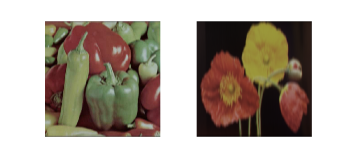
Fig. 3: Example 1: Blurred and noisy images, $\tt peppers$ (left), $\tt papav256$ (right).

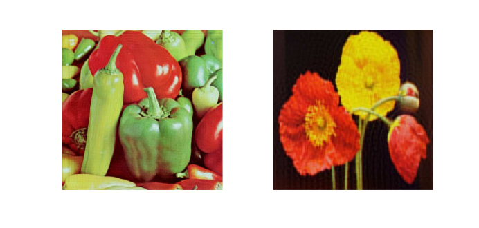
Fig. 4: Example 1: Restored images by Algorithm 4, $\tt peppers$ (left), $\tt papav256$ (right).

Fig. 5: Example 1: Restored images by Algorithm 5, $\tt peppers$ (left), $\tt papav256$ (right).

5.2 Example 2

In this example, we evaluate the effectiveness of Algorithm 4 and Algorithm 5 when applied to the restoration of a color video defined by a sequence of RGB images. Video restoration is the problem of restoring a sequence of $k$ color images (frames). Each frame is represented by a tensor of $n\times n\times 3$ pixels. In the present example, we are interested in restoring 10 consecutive frames of a contaminated video. Note that the processing of such given frames, one at a time, is extremely time consuming. We consider the xylophone video from MATLAB. The video clip is in MP4 format with each frame having $240\times 240$ pixels. The (unknown) blur- and noise-free frames are stored in the tensor $\widehat{\mathscr{X}}\in\mathbb{R}^{240\times 240\times 30}$, obtained by stacking the grayscale images that constitute the three channels of each blurred color frame. These frames are blurred by $\mathscr{A}\star\widehat{\mathscr{X}}\star\mathscr{B}=\widehat{\mathscr{C}}$, where $\mathscr{A}$ and $\mathscr{B}$ are a 3-way tensors such that $\mathscr{A}(:,:,1)=\mathbf{A^{(2)}}$, $\mathscr{B}(:,:,1)=(\mathbf{A^{(1)}})^{T}$ and $\mathscr{A}(:,:,i)=\mathscr{B}(:,:,i)=0$, for $i=2,...,30$, using $\sigma=2$ and $r=4$ to build the blurring matrices. We consider white Gaussian noise of levels $\nu=10^{-3}$ or $\nu=10^{-2}$. Figure 6 shows the 5th exact (original) frame and the contaminated version with noise level $\nu=10^{-3}$, which is to be restored. Table 2 displays the performance of Algorithm 4 and Algorithm 5. In Algorithm 4, we have used as an input for noise level $\nu=10^{-3}$, $\mathscr{C}$, $\mathscr{X}_{0}=\mathscr{O}$, $tol=10^{-6}$, $m=10$ and $\text{Iter}_{\text{max}}=10$.The chosen inner and outer iterations for noise level $\nu=10^{-2}$ were $m=4$ and $\text{Iter}_{\text{max}}=4$, respectively. For the ten outer iterations, minimizing the GCV function produces $\mu_{10}=1.15\times 10^{-5}$. Using Algorithm 5, the discrepancy principle with $\eta=1.1$ have been satisfied after $m=59$ steps of T-GGKB method (Algorithm 3), producing a regularization parameter given by $\mu_{m}=1.06\times 10^{-4}$. For completeness, the restorations obtained with Algorithm 4 and Algorithm 5 are shown on the left-hand and the right-hand side of Figure 7, respectively.

Table 2: Results for Example 2.

Noise level	Method	SNR	Relative error	CPU-time (second)
$10^{-3}$	Algorithm 4	19.97	$4.07\times 10^{-2}$	35.68
	Algorithm 5	19.24	$4.43\times 10^{-2}$	25.52
$10^{-2}$	Algorithm 4	15.17	$7.08\times 10^{-2}$	6.12
	Algorithm 5	15.13	$7.11\times 10^{-2}$	4.40

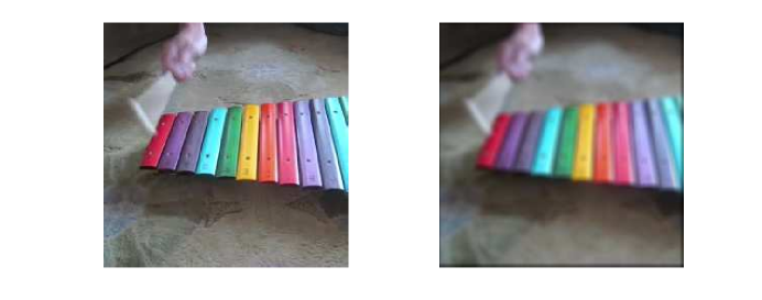
Fig. 6: Example 2: Original frame no. 5 (left), blurred and noisy frame no. 5 (right).

Fig. 7: Example 2: restored frame no. 5 by Algorithm 4 (left), and restored frame no. 5 by Algorithm 5 (right).

6 Conclusion

In this paper we have proposed tensor version of GMRES and Golub–Kahan bidiagonalization algorithms using the T-product, with applications to solving large-scale linear tensor equations arising in the reconstructions of blurred and noisy multichannel images and videos. The numerical experiments that we have performed show the effectiveness of the proposed schemes to inexpensively computing regularized solutions of high quality.

References

- [1] A.H. Bentbib, M. El Guide, K. Jbilou and L. Reichel, Global Golub–Kahan bidiagonalization applied to large discrete ill-posed problems, Journal of Computational and Applied Mathematics, 322(2017), 46–56.
- [2] A.H. Bentbib, M. El Guide, K. Jbilou, E. Onunwor and L. Reichel, Solution methods for linear discrete ill-posed problems for color image restoration, BIT Numerical Mathematics, 58(3)(2018), 555–-576.
- [3] K. Braman, Third-order tensors as linear operators on a space of matrices, Lin. Alg. Appl. 433(2010), 1241–1253.
- [4] M. Brazell, N. Li. C. Navasca, C. Tamon, Solving Multilinear Systems Via Tensor Inversion SIAM J. Matrix Anal. Appl., 34(2)(2013), 542–570
- [5] R. Bouyouli, K. Jbilou, R. Sadaka, H. Sadok, Convergence properties of some block Krylov subspace methods for multiple linear systems, J. Comput. Appl. Math. 196(2006), 498–511.
- [6] F. P. A Beik, F. S. Movahed, S. Ahmadi-Asl, On the Krylov subspace methods based on tensor format for positive definite Sylvester tensor equations, Numer. Lin. Alg. Appl., 23(2016), 444–466.
- [7] F. P. A. Beik, K. Jbilou, M. Najafi-Kalyani and L. Reichel, Golub–Kahan bidiagonalization for ill-conditioned tensor equations with applications. Numerical Algorithms (2020), doi.org/10.1007/s11075-020-00896-8.
- [8] A. Bouhamidi, K. Jbilou, A Sylvester-Tikhonov regularization method for image restauration, J. Compt. Appl. Math., 206(2007), 86–98.
- [9] D. Calvetti, P. C. Hansen, and L. Reichel, L-curve curvature bounds via Lanczos bidiagonalization, Electron. Trans. Numer. Anal., 14(2002), 134–149.
- [10] D. Calvetti and L. Reichel, Tikhonov regularization with a solution constraint, SIAM J. Sci. Comput., 26(2004), 224–239.
- [11] D. Calvetti, G. H. Golub, and L. Reichel, Estimation of the L-curve via Lanczos bidiagonalization, BIT, 39(1999), 603–619.
- [12] M. El Guide, A. El Ichi, K. Jbilou, F.P.A Beik, Tensor GMRES and Golub-Kahan Bidiagonalization methods via the Einstein product with applications to image and video processing, arXiv preprint arXiv:2005.07458.
- [13] G. H. Golub and C. F. Van Loan, Matrix Computations, 3rd ed., Johns Hopkins University Press, Baltimore, 1996.
- [14] G. H. Golub, M. Heath, G. Wahba, Generalized cross-validation as a method for choosing a good ridge parameter, , Technometrics 21(1979), 215–223.
- [15] P. C. Hansen Analysis of discrete ill-posed problems by means of the L-curve, SIAM Rev., 34(1992), 561-580.
- [16] P. C. Hansen Regularization tools, a MATLAB package for analysis of discrete regularization problems, Numer. Algo., 6 (1994), 1-35.
- [17] N. Hao, M. E. Kilmer, K. Braman and R. C. Hoover, Facial recognition using tensor-tensor decompositions, SIAM J. Imaging Sci., 6(2013), 437–463.
- [18] P. C. Hansen, J. Nagy, and D. P. O’Leary, Deblurring Images: Matrices, Spectra, and Filtering, SIAM, Philadelphia, 2006.
- [19] K. Jbilou A. Messaoudi H. Sadok Global FOM and GMRES algorithms for matrix equations, Appl. Num. Math., 31(1999), 49–63.
- [20] K. Jbilou, H. Sadok, and A. Tinzefte, Oblique projection methods for linear systems with multiple right-hand sides, Electron. Trans. Numer. Anal., 20(2005) ,119–138.
- [21] M. N. Kalyani, F. P. A. Beik and K. Jbilou, On global iterative schemes based on Hessenberg process for (ill-posed) Sylvester tensor equations, J. Comput. Appl. Math. 373(2020), 112216.
- [22] T. G. Kolda, B. w. Bader, Tensor Decompositions and Applications. SIAM Rev. 3, 455-500 (2009).
- [23] T. Kolda, B. Bader, Higher-order web link analysis using multilinear algebra, in: Proceedings of the Fifth IEEE International Conference on Data Mining, ICDM 2005, IEEE Computer Society, 2005, pp. 242–-249.
- [24] M.E. Kimler and C.D. Martin Factorization strategies for third-order tensors, Lin. Alg. Appl., 435(2011), 641–-658.
- [25] M.E. Kilmer, C.D. Martin, L. Perrone, A third-order generalization of the matrix svd as a product of third-order tensors, Tech. Report TR-2008-4, Tufts University, Computer Science Department, 2008.
- [26] M. E. Kilmer, K. Braman, N. Hao and R. C. Hoover, Third-order tensors as operators on matrices: a theoretical and computational framework with applications in imaging, SIAM J. Matrix Anal. Appl., 34(2013), 148–172.
- [27] M. Liang, B. Zheng, Further results on Moore–Penrose inverses of tensors with application to tensor nearness problems. Comput. Math. Appl., 77(5)(2019), 1282–1293.
- [28] N. Lee, A. Cichocki, Fundamental tensor operations for large-scale data analysis using tensor network formats, Mult. Sys.t Sig.n Pro., 29(2018), 921–960.
- [29] Qi, L.-Q., Luo, Z.-Y.: Tensor analysis: spectral theory and special tensors. SIAM, Philadelphia, 2017.
- [30] Tensor Robust Principal Component Analysis with A New Tensor Nuclear Norm, IEEE trans. Patt. Anal. Mach. Intel.,
- [31] L. De Lathauwer and A. de Baynast, Blind deconvolution of DS-CDMA signals by means of decomposition in rank-(l, L, L) terms, IEEE Trans. Sign.Proc., 56(2008), 1562–1571.
- [32] Li, X.-T., Ng, M.K.: Solving sparse non-negative tensor equations: algorithms and applications. Front. Math. China 10(3)(2015), 649–-680.
- [33] Luo, Z.-Y., Qi, L.-Q., Xiu, N.-H.: The sparsest solutions to Z-tensor complementarity problems. Optim Lett. 11(2017), 471–-482.
- [34] Y. Miao, L. Qi and Y. Wei, Generalized Tensor Function via the Tensor Singular Value Decomposition based on the T-Product, Lin. Alg. Appl., 590(2020), 258–303.
- [35] L. Sun, B. Zheng, C.Bu, Y.Wei, Moore Penrose inverse of tensors via Einstein product, Lin. Mult. Alg, 64(2016),686–698.
- [36] A.N. Tikhonov, Regularization of incorrectly posed problems, Soviet Math., 4(1963), 1624–1627.
- [37] M. A. O. Vasilescu and D. Terzopoulos, Multilinear analysis of image ensembles: TensorFaces, in ECCV 2002: Proceedings of the 7th European Conference on Computer Vision, Lecture Notes in Comput. Sci. 2350, Springer, 2002, pp. 447-460.
- [38] M. A. O. Vasilescu and D. Terzopoulos, Multilinear image analysis for facial recognition, in ICPR 2002: Proceedings of the 16th International Conference on Pattern Recognition, 2002, pp. 511-514.
- [39] G. Wahba, Pratical approximation solutions to linear operator equations when the data are noisy, SIAM J. Numer. Anal. 14(1977), 651–667.