Sparse and Continuous Attention Mechanisms

Abstract

Exponential families are widely used in machine learning; they include many distributions in continuous and discrete domains (e.g., Gaussian, Dirichlet, Poisson, and categorical distributions via the softmax transformation). Distributions in each of these families have fixed support. In contrast, for finite domains, there has been recent work on sparse alternatives to softmax (e.g. sparsemax and $\alpha$-entmax), which have varying support, being able to assign zero probability to irrelevant categories. This paper expands that work in two directions: first, we extend $\alpha$-entmax to continuous domains, revealing a link with Tsallis statistics and deformed exponential families. Second, we introduce continuous-domain attention mechanisms, deriving efficient gradient backpropagation algorithms for $\alpha\in\{1,2\}$. Experiments on attention-based text classification, machine translation, and visual question answering illustrate the use of continuous attention in 1D and 2D, showing that it allows attending to time intervals and compact regions.

1 Introduction

Exponential families are ubiquitous in statistics and machine learning [1, 2]. They enjoy many useful properties, such as the existence of conjugate priors (crucial in Bayesian inference) and the classical Pitman-Koopman-Darmois theorem [3, 4, 5], which states that, among families with fixed support (independent of the parameters), exponential families are the only having sufficient statistics of fixed dimension for any number of i.i.d. samples.

Departing from exponential families, there has been recent work on discrete, finite-domain distributions with varying and sparse support, via the sparsemax and the entmax transformations [6, 7, 8]. Those approaches drop the link to exponential families of categorical distributions provided by the softmax transformation, which always yields dense probability mass functions. In contrast, sparsemax and entmax can lead to sparse distributions, whose support is not constant throughout the family. This property has been used to design sparse attention mechanisms with improved interpretability [8, 9].

However, sparsemax and entmax are so far limited to discrete domains. Can a similar approach be extended to continuous domains? This paper provides that extension and pinpoints a connection with “deformed exponential families” [10, 11, 12] and Tsallis statistics [13], leading to $\alpha$-sparse families (§2). We use this construction to obtain new density families with varying support, including the truncated parabola and paraboloid distributions (2-sparse counterpart of the Gaussian, §2.4 and Fig. 1).

Softmax and its variants are widely used in attention mechanisms, an important component of neural networks [14]. Attention-based neural networks can “attend” to finite sets of objects and identify relevant features. We use our extension above to devise new continuous attention mechanisms (§3), which can attend to continuous data streams and to domains that are inherently continuous, such as images. Unlike traditional attention mechanisms, ours are suitable for selecting compact regions, such as 1D-segments or 2D-ellipses. We show that the Jacobian of these transformations are generalized covariances, and we use this fact to obtain efficient backpropagation algorithms (§3.2).

As a proof of concept, we apply our models with continuous attention to text classification, machine translation, and visual question answering tasks, with encouraging results (§4).

Notation.

Let $(S,\mathcal{A},\nu)$ be a measure space, where $S$ is a set, $\mathcal{A}$ is a $\sigma$-algebra, and $\nu$ is a measure. We denote by $\mathcal{M}_{+}^{1}(S)$ the set of $\nu$-absolutely continuous probability measures. From the Radon-Nikodym theorem [15, §31], each element of $\mathcal{M}_{+}^{1}(S)$ is identified (up to equivalence within measure zero) with a probability density function $p:S\rightarrow\mathbb{R}_{+}$, with $\int_{S}p(t)\,d\nu(t)=1$. For convenience, we often drop $d\nu(t)$ from the integral. We denote the measure of $A\in\mathcal{A}$ as $|A|=\nu(A)=\int_{A}1$, and the support of a density $p\in\mathcal{M}_{+}^{1}(S)$ as $\mathrm{supp}(p)=\{t\in S\mid p(t)>0\}$. Given $\phi:S\rightarrow\mathbb{R}^{m}$, we write expectations as $\mathbb{E}_{p}[\phi(t)]:=\int_{S}p(t)\,\phi(t)$. Finally, we define $[a]_{+}:=\max\{a,0\}$.

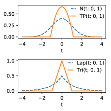
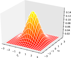
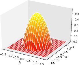
Figure 1: 1D and 2D distributions generated by the $\Omega_{\alpha}$-RPM for $\alpha\in\{1,2\}$. Left: Univariate location-scale families, including Gaussian and truncated parabola (top) and Laplace and triangular (bottom). Middle and right: Bivariate Gaussian $\mathcal{N}(t;0,I)$ and truncated paraboloid $\mathrm{TP}(t;0,I)$.

2 Sparse Families

In this section, we provide background on exponential families and its generalization through Tsallis statistics. We link these concepts, studied in statistical physics, to sparse alternatives to softmax recently proposed in the machine learning literature [6, 8], extending the latter to continuous domains.

2.1 Regularized prediction maps ($\Omega$-RPM)

Our starting point is the notion of $\Omega$-regularized prediction maps, introduced by Blondel et al. [7] for finite domains $S$. This is a general framework for mapping vectors in $\mathbb{R}^{|S|}$ (e.g., label scores computed by a neural network) into probability vectors in $\triangle^{|S|}$ (the simplex), with a regularizer $\Omega$ encouraging uniform distributions. Particular choices of $\Omega$ recover argmax, softmax [16], and sparsemax [6]. Our definition below extends this framework to arbitrary measure spaces $\mathcal{M}_{+}^{1}(S)$, where we assume $\Omega:\mathcal{M}_{+}^{1}(S)\rightarrow\mathbb{R}$ is a lower semi-continuous, proper, and strictly convex function.

The $\Omega$-regularized prediction map ($\Omega$-RPM) $\hat{p}_{\Omega}:\mathcal{F}\rightarrow\mathcal{M}_{+}^{1}(S)$ is defined as

$$\hat{p}_{\Omega}[f]=\operatorname*{arg\,max}_{p\in\mathcal{M}_{+}^{1}(S)}\mathbb{E}_{p}[f(t)]-\Omega(p),$$ (1)

where $\mathcal{F}$ is the set of functions for which the maximizer above exists and is unique.

It is often convenient to consider a “temperature parameter” $\tau>0$, absorbed into $\Omega$ via $\Omega:=\tau\tilde{\Omega}$. If $f$ has a unique global maximizer $t^{\star}$, the low-temperature limit yields ${\lim_{\tau\rightarrow 0}}\,\hat{p}_{\tau\tilde{\Omega}}[f]=\delta_{t^{\star}}$, a Dirac delta distribution at the maximizer of $f$. For finite $S$, this is the argmax transformation shown in [7]. Other interesting examples of regularization functionals are shown in the next subsections.

2.2 Shannon’s negentropy and exponential families

A natural choice of regularizer is the Shannon’s negentropy, $\Omega(p)=\int_{S}p(t)\log p(t)$. In this case, if we interpret $-f(t)$ as an energy function, the $\Omega$-RPM corresponds to the well-known free energy variational principle, leading to Boltzmann-Gibbs distributions ([17]; see App. A):

$$\hat{p}_{\Omega}[f](t)=\frac{\exp(f(t))}{\int_{S}\exp(f(t^{\prime}))d\nu(t^{\prime})}=\exp\bigl{(}f(t)-A(f)\bigr{)},$$ (2)

where $A(f):=\log\int_{S}\exp(f(t))$ is the log-partition function. If $S$ is finite and $\nu$ is the counting measure, the integral in (2) is a summation and we can write $f$ as a vector $[f_{1},\ldots,f_{|S|}]\in\mathbb{R}^{|S|}$. In this case, the $\Omega$-RPM is the softmax transformation,

$$\hat{p}_{\Omega}[f]=\mathrm{softmax}(f)=\tfrac{\exp(f)}{\sum_{k=1}^{|S|}\exp(f_{k})}\in\triangle^{|S|}.$$ (3)

If $S=\mathbb{R}^{N}$, $\nu$ is the Lebesgue measure, and $f(t)=-\nicefrac{{1}}{{2}}(t-\mu)^{\top}\Sigma^{-1}(t-\mu)$ for $\mu\in\mathbb{R}^{N}$ and $\Sigma\succ 0$ (i.e., $\Sigma$ is a positive definite matrix), we obtain a multivariate Gaussian, $\hat{p}_{\Omega}[f](t)=\mathcal{N}(t;\mu,\Sigma)$. This becomes a univariate Gaussian $\mathcal{N}(t;\mu,\sigma^{2})$ if $N=1$. For $S=\mathbb{R}$ and defining $f(t)=-|t-\mu|/b$, with $\mu\in\mathbb{R}$ and $b>0$, we get a Laplace density, $\hat{p}_{\Omega}[f](t)=\tfrac{1}{2b}\exp\left(-|t-\mu|/b\right)$.

Exponential families.

Let $f_{\theta}(t)=\theta^{\top}\phi(t)$, where $\phi(t)\in\mathbb{R}^{M}$ is a vector of statistics and $\theta\in\Theta\subseteq\mathbb{R}^{M}$ is a vector of canonical parameters. A family of the form (2) parametrized by $\theta\in\Theta\subseteq\mathbb{R}^{M}$ is called an exponential family [2]. Exponential families have many appealing properties, such as the existence of conjugate priors and sufficient statistics, and a dually flat geometric structure [18]. Many well-known distributions are exponential families, including the categorical and Gaussian distributions above, and Laplace distributions with a fixed $\mu$. A key property of exponential families is that the support is constant within the same family and dictated by the base measure $\nu$: this follows immediately from the positiveness of the $\exp$ function in (2). We abandon this property in the sequel.

2.3 Tsallis’ entropies and $\alpha$-sparse families

Motivated by applications in statistical physics, Tsallis [13] proposed a generalization of Shannon’s negentropy. This generalization is rooted on the notions of $\beta$-logarithm, $\log_{\beta}:\mathbb{R}_{\geq 0}\rightarrow\mathbb{R}$ (not to be confused with base-$\beta$ logarithm), and $\beta$-exponential, $\exp_{\beta}:\mathbb{R}\rightarrow\mathbb{R}$:

$$\log_{\beta}(u):=\left\{\begin{array}[]{ll}\frac{u^{1-\beta}-1}{1-\beta},&\beta\neq 1\\ \log u,&\beta=1;\end{array}\right.\qquad\exp_{\beta}(u):=\left\{\begin{array}[]{ll}[1+(1-\beta)u]_{+}^{1/(1-\beta)},&\beta\neq 1\\ \exp u,&\beta=1.\end{array}\right.$$ (4)

Note that ${\lim_{\beta\rightarrow 1}}\log_{\beta}(u)=\log u$, ${\lim_{\beta\rightarrow 1}}\exp_{\beta}(u)=\exp u$, and $\log_{\beta}(\exp_{\beta}(u))=u$ for any $\beta$. Another important concept is that of “$\beta$-escort distribution” [13]: this is the distribution $\tilde{p}^{\beta}$ given by

$$\tilde{p}^{\beta}(t):=\frac{p(t)^{\beta}}{\|p\|_{\beta}^{\beta}},\quad\text{where $\|p\|_{\beta}^{\beta}=\int_{S}p(t^{\prime})^{\beta}d\nu(t^{\prime})$}.$$ (5)

Note that we have $\tilde{p}^{1}(t)=p(t)$.

The $\alpha$-Tsallis negentropy [19, 13] is defined as:

$$\Omega_{\alpha}(p):=\tfrac{1}{\alpha}\mathbb{E}_{p}[\log_{2-\alpha}(p(t))]=\begin{cases}\frac{1}{\alpha(\alpha-1)}\left(\int_{S}p(t)^{\alpha}-1\right),&\alpha\neq 1,\\ \int_{S}p(t)\log p(t),&\alpha=1.\end{cases}$$ (6)

Note that $\lim_{\alpha\rightarrow 1}\Omega_{\alpha}(p)=\Omega_{1}(p)$, for any $p\in\mathcal{M}_{+}^{1}(S)$, with $\Omega_{1}(p)$ recovering Shannon’s negentropy (proof in App. B). Another notable case is $\Omega_{2}(p)=\nicefrac{{1}}{{2}}\int_{S}p(t)^{2}-\nicefrac{{1}}{{2}}$, the negative of which is called the Gini-Simpson index [20, 21]. We come back to the $\alpha=2$ case in §2.4.

For $\alpha>0$, $\Omega_{\alpha}$ is strictly convex, hence it can be plugged in as the regularizer in Def. 2.1. The next proposition ([10]; proof in App. B) provides an expression for $\Omega_{\alpha}$-RPM using the $\beta$-exponential (4):

For $\alpha>0$ and $f\in\mathcal{F}$,

$$\hat{p}_{\Omega_{\alpha}}[f](t)=\exp_{2-\alpha}(f(t)-A_{\alpha}(f)),$$ (7)

where $A_{\alpha}:\mathcal{F}\rightarrow\mathbb{R}$ is a normalizing function: $A_{\alpha}(f)=\frac{\frac{1}{1-\alpha}+\int_{S}p_{\theta}(t)^{2-\alpha}f(t)}{\int_{S}p_{\theta}(t)^{2-\alpha}}-\frac{1}{1-\alpha}.$

Let us contrast (7) with Boltzmann-Gibbs distributions (2), recovered with $\alpha=1$. One key thing to note is that the $(2-\alpha)$-exponential, for $\alpha>1$, can return zero values. Therefore, the distribution $\hat{p}_{\Omega_{\alpha}}[f]$ in (7) may not have full support, i.e., we may have $\mathrm{supp}(\hat{p}_{\Omega_{\alpha}}[f])\subsetneq S$. We say that $\hat{p}_{\Omega_{\alpha}}[f]$ has sparse support if $\nu(S\setminus\mathrm{supp}(\hat{p}_{\Omega_{\alpha}}[f]))>0$. This generalizes the notion of sparse vectors.

Relation to sparsemax and entmax.

Blondel et al. [7] showed that, for finite $S$, $\Omega_{2}$-RPM is the sparsemax transformation, $\hat{p}_{\Omega}[f]=\mathrm{sparsemax}(f)=\arg\min_{p\in\triangle^{|S|}}\|p-f\|^{2}$. Other values of $\alpha$ were studied by Peters et al. [8], under the name $\alpha$-entmax transformation. For $\alpha>1$, these transformations have a propensity for returning sparse distributions, where several entries have zero probability. Proposition 2.3 shows that similar properties can be obtained when $S$ is continuous.

Deformed exponential families.

With a linear parametrization $f_{\theta}(t)=\theta^{\top}\phi(t)$, distributions with the form (7) are called deformed exponential or $q$-exponential families [10, 11, 12, 24]. The geometry of these families induced by the Tsallis $q$-entropy was studied by Amari [18, §4.3]. Unlike those prior works, we are interested in the sparse, light tail scenario ($\alpha>1$), not in heavy tails. For $\alpha>1$, we call these $\alpha$-sparse families. When $\alpha\rightarrow 1$, $\alpha$-sparse families become exponential families and they cease to be “sparse”, in the sense that all distributions in the same family have the same support.

A relevant problem is that of characterizing $A_{\alpha}(\theta)$. When $\alpha=1$, $A_{1}(\theta)={\lim_{\alpha\rightarrow 1}}A_{\alpha}(\theta)=\log\int_{S}\exp(\theta^{\top}\phi(t))$ is the log-partition function (see (2)), and its first and higher order derivatives are equal to the moments of the sufficient statistics. The following proposition (stated as Amari and Ohara [25, Theorem 5], and proved in our App. D) characterizes $A_{\alpha}(\theta)$ for $\alpha\neq 1$ in terms of an expectation under the $\beta$-escort distribution for $\beta=2-\alpha$ (see (5)). This proposition will be used later to derive the Jacobian of entmax attention mechanisms.

$A_{\alpha}(\theta)$ is a convex function and its gradient is given by

$$\nabla_{\theta}A_{\alpha}(\theta)=\mathbb{E}_{\tilde{p}_{\theta}^{2-\alpha}}[\phi(t)]=\frac{\int_{S}p_{\theta}(t)^{2-\alpha}\phi(t)}{\int_{S}p_{\theta}(t)^{2-\alpha}}.$$ (8)

2.4 The 2-Tsallis entropy: sparsemax

In this paper, we focus on the case $\alpha=2$. For finite $S$, this corresponds to the sparsemax transfomation proposed by Martins and Astudillo [6], which has appealing theoretical and computational properties. In the general case, plugging $\alpha=2$ in (7) leads to the $\Omega_{2}$-RPM,

$$\hat{p}_{\Omega_{2}}[f](t)=[f(t)-\lambda]_{+},\qquad\text{where $\lambda=A_{2}(f)-1$,}$$ (9)

i.e., $\hat{p}_{\Omega_{2}}[f]$ is obtained from $f$ by subtracting a constant (which may be negative) and truncating, where that constant $\lambda$ must be such that $\int_{S}[f(t)-\lambda]_{+}=1$.

If $S$ is continuous and $\nu$ the Lebesgue measure, we call $\Omega_{2}$-RPM the continuous sparsemax transformation. Examples follow, some of which correspond to novel distributions.

Truncated parabola.

If $f(t)=-\frac{(t-\mu)^{2}}{2\sigma^{2}}$, we obtain the continuous sparsemax counterpart of a Gaussian, which we dub a “truncated parabola”:

$$\hat{p}_{\Omega_{2}}[f](t)=\left[-\tfrac{(t-\mu)^{2}}{2\sigma^{2}}-\lambda\right]_{+}\eqqcolon\mathrm{TP}(t;\mu,\sigma^{2}),$$ (10)

where $\lambda=-\tfrac{1}{2}\bigl{(}3/(2\sigma)\bigr{)}^{2/3}$ (see App. E.1). This function, depicted in Fig. 1 (top left), is widely used in density estimation. For $\mu=0$ and $\sigma=\sqrt{2/3}$, it is known as the Epanechnikov kernel [26].

Truncated paraboloid.

The previous example can be generalized to $S=\mathbb{R}^{N}$, with $f(t)=-\frac{1}{2}(t-\mu)^{\top}\Sigma^{-1}(t-\mu)$, where $\Sigma\succ 0$, leading to a “multivariate truncated paraboloid,” the sparsemax counterpart of the multivariate Gaussian (see middle and rightmost plots in Fig. 1):

$$\hat{p}_{\Omega_{2}}[f](t)=\bigl{[}-\lambda-\tfrac{1}{2}(t-\mu)\Sigma^{-1}(t-\mu)\bigr{]}_{+},\qquad\text{where $\lambda=-\Bigl{(}\Gamma\bigl{(}\tfrac{N}{2}+2\bigr{)}/\sqrt{\mathrm{det}(2\pi\Sigma)}\Bigr{)}^{\frac{2}{2+N}}$}.$$ (11)

The expression above, derived in App. E.2, reduces to (10) for $N=1$. Notice that (unlike in the Gaussian case) a diagonal $\Sigma$ does not lead to a product of independent truncated parabolas.

Triangular.

Setting $f(t)=-|t-\mu|/b$, with $b>0$, yields the triangular distribution

$$\hat{p}_{\Omega_{2}}[f](t)=\left[-\lambda-\tfrac{|t-\mu|}{b}\right]_{+}\eqqcolon\mathrm{Tri}(t;\mu,b),$$ (12)

where $\lambda\!=\!-1/\sqrt{b}$ (see App. E.3). Fig. 1 (bottom left) depicts this distribution alongside Laplace.

Location-scale families.

More generally, let $f_{\mu,\sigma}(t):=-\frac{1}{\sigma}g^{\prime}(|t-\mu|/\sigma)$ for a location $\mu\in\mathbb{R}$ and a scale $\sigma>0$, where $g:\mathbb{R}_{+}\rightarrow\mathbb{R}$ is convex and continuously differentiable. Then, we have

$$\hat{p}_{\Omega_{2}}[f](t)=\left[-\lambda-\tfrac{1}{\sigma}g^{\prime}(|t-\mu|/\sigma)\right]_{+},$$ (13)

where $\lambda=-g^{\prime}(a)/\sigma$ and $a$ is the solution of the equation $ag^{\prime}(a)-g(a)+g(0)=\frac{1}{2}$ (a sufficient condition for such solution to exist is $g$ being strongly convex; see App. E.4 for a proof). This example subsumes the truncated parabola ($g(t)=t^{3}/6$) and the triangular distribution ($g(t)=t^{2}/2$).

2-sparse families.

Truncated parabola and paraboloid distributions form a 2-sparse family, with statistics $\phi(t)=[t,\mathrm{vec}(tt^{\top})]$ and canonical parameters $\theta=[\Sigma^{-1}\mu,\mathrm{vec}(-\frac{1}{2}\Sigma^{-1})]$. Gaussian distributions form an exponential family with the same sufficient statistics and canonical parameters. In 1D, truncated parabola and Gaussians are both particular cases of the so-called “$q$-Gaussian” [10, §4.1], for $q=2-\alpha$. Triangular distributions with a fixed location $\mu$ and varying scale $b$ also form a 2-sparse family (similarly to Laplace distributions with fixed location being exponential families).

3 Continuous Attention

Attention mechanisms have become a key component of neural networks [14, 27, 28]. They dynamically detect and extract relevant input features (such as words in a text or regions of an image). So far, attention has only been applied to discrete domains; we generalize it to continuous spaces.

Discrete attention.

Assume an input object split in $L=|S|$ pieces, e.g., a document with $L$ words or an image with $L$ regions. A vanilla attention mechanism works as follows: each piece has a $D$-dimensional representation (e.g., coming from an RNN or a CNN), yielding a matrix $V\in\mathbb{R}^{D\times L}$. These representations are compared against a query vector (e.g., using an additive model [14]), leading to a score vector $f=[f_{1},\ldots,f_{L}]\in\mathbb{R}^{L}$. Intuitively, the relevant pieces that need attention should be assigned high scores. Then, a transformation $\rho:\mathbb{R}^{L}\rightarrow\triangle^{L}$ (e.g., softmax or sparsemax) is applied to the score vector to produce a probability vector $p=\rho(f)$. We may see this as an $\Omega$-RPM. The probability vector $p$ is then used to compute a weighted average of the input representations, via $c=Vp\in\mathbb{R}^{D}$. This context vector $c$ is finally used to produce the network’s decision.

To learn via the backpropagation algorithm, the Jacobian of the transformation $\rho$, $J_{\rho}\in\mathbb{R}^{L\times L}$, is needed. Martins and Astudillo [6] gave expressions for softmax and sparsemax,

$$J_{\mathrm{softmax}}(f)=\mathrm{Diag}(p)-pp^{\top},\qquad J_{\mathrm{sparsemax}}(f)=\mathrm{Diag}(s)-ss^{\top}/(1^{\top}s),$$ (14)

where $p=\mathrm{softmax}(f)$, and $s$ is a binary vector whose $\ell$^th entry is 1 iff $\ell\in\mathrm{supp}(\mathrm{sparsemax}(f))$.

3.1 The continuous case: score and value functions

Our extension of $\Omega$-RPMs to arbitrary domains (Def. 2.1) opens the door for constructing continuous attention mechanisms. The idea is simple: instead of splitting the input object into a finite set of pieces, we assume an underlying continuous domain: e.g., text may be represented as a function $V:S\rightarrow\mathbb{R}^{D}$ that maps points in the real line ($S\subseteq\mathbb{R}$, continuous time) onto a $D$-dimensional vector representation, representing the “semantics” of the text evolving over time; images may be regarded as a smooth function in 2D ($S\subseteq\mathbb{R}^{2}$), instead of being split into regions in a grid.

Instead of scores $[f_{1},\ldots,f_{L}]$, we now have a score function $f:S\rightarrow\mathbb{R}$, which we map to a probability density $p\in\mathcal{M}_{+}^{1}(S)$. This density is used in tandem with the value mapping $V:S\rightarrow\mathbb{R}^{D}$ to obtain a context vector $c=\mathbb{E}_{p}[V(t)]\in\mathbb{R}^{D}$. Since $\mathcal{M}_{+}^{1}(S)$ may be infinite dimensional, we need to parametrize $f$, $p$, and $V$ to be able to compute in a finite-dimensional parametric space.

Building attention mechanisms.

We represent $f$ and $V$ using basis functions, $\phi:S\rightarrow\mathbb{R}^{M}$ and $\psi:S\rightarrow\mathbb{R}^{N}$, defining $f_{\theta}(t)=\theta^{\top}\phi(t)$ and $V_{B}(t)=B\psi(t)$, where $\theta\in\mathbb{R}^{M}$ and $B\in\mathbb{R}^{D\times N}$. The score function $f_{\theta}$ is mapped into a probability density $p:=\hat{p}_{\Omega}[f_{\theta}]$, from which we compute the context vector as $c=\mathbb{E}_{p}[V_{B}(t)]=Br$, with $r=\mathbb{E}_{p}[\psi(t)]$. Summing up yields the following: Let $\langle S,\Omega,\phi,\psi\rangle$ be a tuple with $\Omega:\mathcal{M}_{+}^{1}(S)\rightarrow\mathbb{R}$, $\phi:S\rightarrow\mathbb{R}^{M}$, and $\psi:S\rightarrow\mathbb{R}^{N}$. An attention mechanism is a mapping $\rho:\Theta\subseteq\mathbb{R}^{M}\rightarrow\mathbb{R}^{N}$, defined as:

$$\rho(\theta)=\mathbb{E}_{p}[\psi(t)],$$ (15)

with $p=\hat{p}_{\Omega}[f_{\theta}]$ and $f_{\theta}(t)=\theta^{\top}\phi(t)$. If $\Omega=\Omega_{\alpha}$, we call this entmax attention, denoted as $\rho_{\alpha}$. The values $\alpha=1$ and $\alpha=2$ lead to softmax and sparsemax attention, respectively.

Note that, if $S=\{1,...,L\}$ and $\phi(k)=\psi(k)=e_{k}$ (Euclidean canonical basis), we recover the discrete attention of Bahdanau et al. [14]. Still in the finite case, if $\phi(k)$ and $\psi(k)$ are key and value vectors and $\theta$ is a query vector, this recovers the key-value attention of Vaswani et al. [28].

On the other hand, for $S=\mathbb{R}^{D}$ and $\phi(t)=[t,\mathrm{vec}(tt^{\top})]$, we obtain new attention mechanisms (assessed experimentally for the 1D and 2D cases in §4): for $\alpha=1$, the underlying density $p$ is Gaussian, and for $\alpha=2$, it is a truncated paraboloid (see §2.4). In both cases, we show (App. G) that the expectation (15) is tractable (1D) or simple to approximate numerically (2D) if $\psi$ are Gaussian RBFs, and we use this fact in §4 (see Alg. 1 for pseudo-code for the case $\alpha=1$).

Parameters: Gaussian RBFs $\psi(t)=[\mathcal{N}(t;\mu_{j},\Sigma_{j})]_{j=1}^{N}$, basis functions $\phi(t)=[t,\mathrm{vec}(tt^{\top})]$, value function $V_{B}(t)=B\psi(t)$ with $B\in\mathbb{R}^{D\times N}$, score function $f_{\theta}(t)=\theta^{\top}\phi(t)$ with $\theta\in\mathbb{R}^{M}$

Function Forward($\theta:=[\Sigma^{-1}\mu,-\frac{1}{2}\Sigma^{-1}]$):

       $r_{j}\leftarrow\mathbb{E}_{\hat{p}_{\Omega}[f_{\theta}]}[\psi_{j}(t)]=\mathcal{N}(\mu,\mu_{j},\Sigma+\Sigma_{j}),\quad\forall j\in[N]$ // Eqs. 15, 46

      return $c\leftarrow Br$ (context vector)

Function Backward($\frac{\partial\mathcal{L}}{\partial c},\theta:=[\Sigma^{-1}\mu,-\frac{1}{2}\Sigma^{-1}]$):

       for $j\leftarrow 1$ to $N$ do

             $\tilde{s}\leftarrow\mathcal{N}(\mu,\mu_{j},\Sigma+\Sigma_{j}),\,\,\tilde{\Sigma}\leftarrow(\Sigma^{-1}+\Sigma_{j}^{-1})^{-1},\,\,\tilde{\mu}\leftarrow\tilde{\Sigma}(\Sigma^{-1}\mu+\Sigma_{j}^{-1}\mu_{j})$

             $\frac{\partial r_{j}}{\partial\theta}\leftarrow\mathrm{cov}_{\hat{p}_{\Omega}[f_{\theta}]}(\phi(t),\psi_{j}(t))=[\tilde{s}(\tilde{\mu}-\mu);\tilde{s}(\tilde{\Sigma}+\tilde{\mu}\tilde{\mu}^{\top}-\Sigma-\mu\mu^{\top})]$ // Eqs. 18, 47--48

            

      return $\frac{\partial\mathcal{L}}{\partial\theta}\leftarrow\left(\frac{\partial r}{\partial\theta}\right)^{\top}B^{\top}\frac{\partial\mathcal{L}}{\partial c}$

Algorithm 1 Continuous softmax attention with $S=\mathbb{R}^{D}$, $\Omega=\Omega_{1}$, and Gaussian RBFs.

Defining the value function $V_{B}(t)$.

In many problems, the input is a discrete sequence of observations (e.g., text) or it was discretized (e.g., images), at locations $\{t_{\ell}\}_{\ell=1}^{L}$. To turn it into a continuous signal, we need to smooth and interpolate these observations. If we start with a discrete encoder representing the input as a matrix $H\in\mathbb{R}^{D\times L}$, one way of obtaining a value mapping $V_{B}:S\rightarrow\mathbb{R}^{D}$ is by “approximating” $H$ with multivariate ridge regression. With $V_{B}(t)=B\psi(t)$, and packing the basis vectors $\psi(t_{\ell})$ as columns of matrix $F\in\mathbb{R}^{N\times L}$, we obtain:

$$B^{\star}\,\,=\,\,\arg\min_{B}\|BF-H\|_{F}^{2}+\lambda\|B\|_{F}^{2}\,\,=\,\,HF^{\top}(FF^{\top}+\lambda I_{N})^{-1}\,\,=\,\,HG,$$ (16)

where $\|.\|_{F}$ is the Frobenius norm, and the $L\times N$ matrix $G=F^{\top}(FF^{\top}+\lambda I_{N})^{-1}$ depends only on the values of the basis functions at discrete time steps and can be obtained off-line for different input lenghts $L$. The result is an expression for $V_{B}$ with $ND$ coefficients, cheaper than $H$ if $N\ll L$.

3.2 Gradient backpropagation with continuous attention

The next proposition, based on Proposition 2.3 and proved in App. F, allows backpropagating over continuous entmax attention mechanisms. We define, for $\beta\geq 0$, a generalized $\beta$-covariance,

$$\mathrm{cov}_{p,\beta}[\phi(t),\psi(t)]\,\,=\,\,\|p\|_{\beta}^{\beta}\times\left(\mathbb{E}_{\tilde{p}_{\beta}}\big{[}\phi(t)\psi(t)^{\top}\big{]}-\mathbb{E}_{\tilde{p}_{\beta}}[\phi(t)]\,\mathbb{E}_{\tilde{p}_{\beta}}[\psi(t)]^{\top}\right),$$ (17)

where $\tilde{p}_{\beta}$ is the $\beta$-escort distribution in (5). For $\beta=1$, we have the usual covariance; for $\beta=0$, we get a covariance taken w.r.t. a uniform density on the support of $p$, scaled by $|\mathrm{supp}(p)|$.

Let $p=\hat{p}_{\Omega_{\alpha}}[f_{\theta}]$ with $f_{\theta}(t)=\theta^{\top}\phi(t)$. The Jacobian of the $\alpha$-entmax is:

$$J_{\rho_{\alpha}}(\theta)=\frac{\partial\rho_{\alpha}(\theta)}{\partial\theta}=\mathrm{cov}_{p,2-\alpha}(\phi(t),\psi(t)).$$ (18)

Note that in the finite case, (18) reduces to the expressions in (14) for softmax and sparsemax.

Example: Gaussian RBFs.

As before, let $S=\mathbb{R}^{D}$, $\phi(t)=[t,\mathrm{vec}(tt^{\top})]$, and $\psi_{j}(t)=\mathcal{N}(t;\mu_{j},\Sigma_{j})$. For $\alpha=1$, we obtain closed-form expressions for the expectation (15) and the Jacobian (18), for any $D\in\mathbb{N}$: $\hat{p}_{\Omega}[f_{\theta}]$ is a Gaussian, the expectation (15) is the integral of a product of Gaussians, and the covariance (18) involves first- and second-order Gaussian moments. Pseudo-code for the case $\alpha=1$ is shown as Alg. 1. For $\alpha=2$, $\hat{p}_{\Omega}[f_{\theta}]$ is a truncated paraboloid. In the 1D case, both (15) and (18) can be expressed in closed form in terms of the $\mathrm{erf}$ function. In the 2D case, we can reduce the problem to 1D integration using the change of variable formula and working with polar coordinates. See App. G for details.

We use the facts above in the experimental section (§4), where we experiment with continuous variants of softmax and sparsemax attentions in natural language processing and vision applications.

4 Experiments

As proof of concept, we test our continuous attention mechanisms on three tasks: document classification, machine translation, and visual question answering (more experimental details in App. H).

Document classification.

Although textual data is fundamentally discrete, modeling long documents as a continuous signal may be advantageous, due to smoothness and independence of length. To test this hypothesis, we use the IMDB movie review dataset [29], whose inputs are documents (280 words on average) and outputs are sentiment labels (positive/negative). Our baseline is a biLSTM with discrete attention. For our continuous attention models, we normalize the document length $L$ into the unit interval $[0,1]$, and use $f(t)\!=\!\nicefrac{{-(t-\mu)^{2}}}{{2\sigma^{2}}}$ as the score function, leading to a 1D Gaussian ($\alpha=1$) or truncated parabola ($\alpha=2$) as the attention density. We compare three attention variants: discrete attention with softmax [14] and sparsemax [6]; continuous attention, where a CNN and max-pooling yield a document representation $v$ from which we compute $\mu=\mathrm{sigmoid}(w_{1}^{\top}v)$ and $\sigma^{2}=\mathrm{softplus}(w_{2}^{\top}v)$; and combined attention, which obtains $p\in\triangle^{L}$ from discrete attention, computes $\mu=\mathbb{E}_{p}[\ell/L]$ and $\sigma^{2}=\mathbb{E}_{p}[(\ell/L)^{2}]-\mu^{2}$, applies the continuous attention, and sums the two context vectors (this model has the same number of parameters as the discrete attention baseline).

Table 1: Results on IMDB in terms of accuracy (%). For the continuous attentions, we used $N\in\{32,64,128\}$ Gaussian RBFs $\mathcal{N}(t,\tilde{\mu},\tilde{\sigma}^{2})$, with $\tilde{\mu}$ linearly spaced in $[0,1]$ and $\tilde{\sigma}\in\{.1,.5\}$.

Attention	$\bar{L}\approx 280$
Discrete softmax	90.78
Discrete sparsemax	90.58

Attention	$N=32$	$N=64$	$N=128$
Continuous softmax	90.20	90.68	90.52
Continuous sparsemax	90.52	89.63	90.90
Disc. + Cont. softmax	90.98	90.69	89.62
Disc. + Cont. sparsemax	91.10	91.18	90.98

Table 1 shows accuracies for different numbers $N$ of Gaussian RBFs. The accuracies of the individual models are similar, suggesting that continuous attention is as effective as its discrete counterpart, despite having fewer basis functions than words, i.e., $N\ll L$. Among the continuous variants, the sparsemax outperforms the softmax, except for $N=64$. We also see that a large $N$ is not necessary to obtain good results, which is encouraging for tasks with long sequences. Finally, combining discrete and continuous sparsemax produced the best results, without increasing the number of parameters.

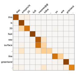
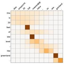
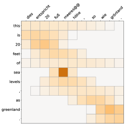
Figure 2: Attention maps in machine translation: discrete (left), continuous softmax (middle), and continuous sparsemax (right), for a sentence in the De-En IWSLT17 validation set. In the rightmost plot, the selected words are the ones with positive density. In the test set, these models attained BLEU scores of 23.92 (discrete), 24.00 (continuous softmax), and 24.25 (continuous sparsemax).

Machine translation.

We use the De$\to$En IWSLT 2017 dataset [30], and a biLSTM model with discrete softmax attention as a baseline. For the continuous attention models, we use the combined attention setting described above, with 30 Gaussian RBFs and $\tilde{\mu}$ linearly spaced in $[0,1]$ and $\tilde{\sigma}\in\{.03,.1,.3\}$. The results (caption of Fig. 2) show a slight benefit in the combined attention over discrete attention only, without any additional parameters. Fig. 2 shows heatmaps for the different attention mechanisms on a De$\to$En sentence. The continuous mechanism tends to have attention means close to the diagonal, adjusting the variances based on alignment confidence or when a larger context is needed (e.g., a peaked density for the target word “sea”, and a flat one for “of”).

Visual QA.

Finally, we report experiments with 2D continuous attention on visual question answering, using the VQA-v2 dataset [31] and a modular co-attention network as a baseline [32]. The discrete attention model attends over a 14$\times$14 grid. For continuous attention, we normalize the image size into the unit square $[0,1]^{2}$. We fit a 2D Gaussian ($\alpha=1$) or truncated paraboloid ($\alpha=2$) as the attention density; both correspond to $f(t)=-\frac{1}{2}(t-\mu)^{\top}\Sigma^{-1}(t-\mu)$, with $\Sigma\succ 0$. We use the mean and variance according to the discrete attention probabilities and obtain $\mu$ and $\Sigma$ with moment matching. We use $N=100\ll 14^{2}$ Gaussian RBFs, with $\tilde{\mu}$ linearly spaced in $[0,1]^{2}$ and $\tilde{\Sigma}=0.001\cdot\mathrm{I}$. Overall, the number of neural network parameters is the same as in discrete attention.

The results in Table 2 show similar accuracies for all attention models, with a slight advantage for continuous softmax. Figure 3 shows an example (see App. H for more examples and some failure cases): in the baseline model, the discrete attention is too scattered, possibly mistaking the lamp with a TV screen. The continuous attention models focus on the right region and answer the question correctly, with continuous sparsemax enclosing all the relevant information in its supporting ellipse.

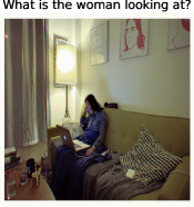
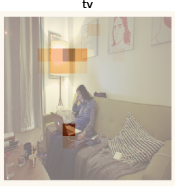
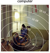
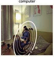
Figure 3: Attention maps for an example in VQA-v2: original image, discrete attention, continuous softmax, and continuous sparsemax. The latter encloses all probability mass within the outer ellipse.

Table 2: Accuracies of different models on the test-dev and test-standard splits of VQA-v2.

Attention	Test-Dev				Test-Standard
	Yes/No	Number	Other	Overall	Yes/No	Number	Other	Overall
Discrete softmax	83.40	43.59	55.91	65.83	83.47	42.99	56.33	66.13
2D continuous softmax	83.40	44.80	55.88	65.96	83.79	44.33	56.04	66.27
2D continuous sparsemax	83.10	44.12	55.95	65.79	83.38	43.91	56.14	66.10

5 Related Work

Relation to the Tsallis maxent principle.

Our paper unifies two lines of work: deformed exponential families from statistical physics [13, 10, 25], and sparse alternatives to softmax recently proposed in the machine learning literature [6, 8, 7], herein extended to continuous domains. This link may be fruitful for future research in both fields. While most prior work is focused on heavy-tailed distributions ($\alpha<1$), we focus instead on light-tailed, sparse distributions, the other side of the spectrum ($\alpha>1$). See App. C for the relation to the Tsallis maxent principle.

Continuity in other architectures and dimensions.

In our paper, we consider attention networks exhibiting temporal/spatial continuity in the input data, be it text (1D) or images (2D). Recent work propose continuous-domain CNNs for 3D structures like point clouds and molecules [34, 35]. The dynamics of continuous-time RNNs have been studied in [36], and similar ideas have been applied to irregularly sampled time series [37]. Other recently proposed frameworks produce continuous variants in other dimensions, such as network depth [38], or in the target domain for machine translation tasks [39]. Our continuous attention networks can be used in tandem with these frameworks.

Gaussian attention probabilities.

Cordonnier et al. [40] analyze the relationship between (discrete) attention and convolutional layers, and consider spherical Gaussian attention probabilities as relative positional encodings. By contrast, our approach removes the need for positional encodings: by converting the input to a function on a predefined continuous space, positions are encoded implicitly, not requiring explicit positional encoding. Gaussian attention has also been hard-coded as input-agnostic self-attention layers in transformers for machine translation tasks by You et al. [41]. Finally, in their DRAW architecture for image generation, Gregor et al. [42, §3.1] propose a selective attention component which is parametrized by a spherical Gaussian distribution.

6 Conclusions and Future Work

We proposed extensions to regularized prediction maps, originally defined on finite domains, to arbitrary measure spaces (§2). With Tsallis $\alpha$-entropies for $\alpha>1$, we obtain sparse families, whose members can have zero tails, such as triangular or truncated parabola distributions. We then used these distributions to construct continuous attention mechanisms (§3). We derived their Jacobians in terms of generalized covariances (Proposition 3.2), allowing for efficient forward and backward propagation. Experiments for 1D and 2D cases were shown on attention-based text classification, machine translation, and visual question answering (§4), with encouraging results.

There are many avenues for future work. As a first step, we considered unimodal distributions only (Gaussian, truncated paraboloid), for which we show that the forward and backpropagation steps have closed form or can be reduced to 1D integration. However, there are applications in which multiple attention modes are desirable. This can be done by considering mixtures of distributions, multiple attention heads, or sequential attention steps. Another direction concerns combining our continuous attention models with other spatial/temporal continuous architectures for CNNs and RNNs [34, 35, 36] or with continuity in other dimensions, such as depth [38] or output space [39].

Broader Impact

We discuss the broader impact of our work, including ethical aspects and future societal consequences. Given the early stage of our work and its predominantly theoretical nature, the discussion is mostly speculative.

The continuous attention models developed in our work can be used in a very wide range of applications, including natural language processing, computer vision, and others. For many of these applications, current state-of-the-art models use discrete softmax attention, whose interpretation capabilities have been questioned in prior work [43, 44, 45]. Our models can potentially lead to more interpretable decisions, since they lead to less scattered attention maps (as shown in our Figures 2–3) and are able to select contiguous text segments or image regions. As such, they may provide better inductive bias for interpretation.

In addition, our attention densities using Gaussian and truncated paraboloids include a variance term, being potentially useful as a measure of confidence—for example, a large ellipse in an image may indicate that the model had little confidence about where it should attend to answer a question, while a small ellipse may denote high confidence on a particular object.

We also see opportunities for research connecting our work with other continuous models [34, 35, 38] leading to end-to-end continuous models which, by avoiding discretization, have the potential to be less susceptible to adversarial attacks via input perturbations. Outside the machine learning field, the links drawn in §2 between sparse alternatives to softmax and models used in non-extensive (Tsallis) statistical physics suggest a potential benefit in that field too.

Note, however, that our work is a first step into all these directions, and as such further investigation will be needed to better understand the potential benefits. We strongly recommend carrying out user studies before deploying any such system, to better understand the benefits and risks. Some of the examples in App. H may help understand potential failure modes.

We should also take into account that, for any computer vision model, there are important societal risks related to privacy-violating surveillance applications. Continuous attention holds the promise to scale to larger and multi-resolution images, which may, in the longer term, be deployed in such undesirable domains. Ethical concerns hold for natural language applications such as machine translation, where biases present in data can be arbitrarily augmented or hidden by machine learning systems. For example, our natural language processing experiments mostly use English datasets (as a target language in machine translation, and in document classification). Further work is needed to understand if our findings generalize to other languages. Likewise, in the vision experiments, the VQA-v2 dataset uses COCO images, which have documented biases [46]. In line with the fundamental scope and early stage of this line of research, we deliberately choose applications on standard benchmark datasets, in an attempt to put as much distance as possible from malevolent applications. Finally, although we chose the most widely used evaluation metrics for each task (accuracy for document classification and visual question answering, BLEU for machine translation), these metrics do not always capture performance quality—for example, BLEU in machine translation is far from being a perfect metric.

The data, memory, and computation requirements for training systems with continuous attention do not seem considerably higher than the ones which use discrete attention. On the other hand, for NLP applications, our approach has the potential to better compress sequential data, by using fewer basis functions than the sequence length (as suggested by our document classification experiments). While there is nothing specific about our research that poses environmental concerns or that promises to alleviate such concerns, our models share the same problematic property as other neural network models in terms of their energy consumption to train models and tune hyperparameters [47].

Supplemental Material

Appendix A Differential Negentropy and Boltzmann-Gibbs distributions

We adapt a proof from Cover and Thomas [17]. Let $\Omega$ be the Shannon negentropy, which is proper, lower semi-continuous, and strictly convex [48, example 9.41], and let

$$\mathrm{KL}(p\|q):=\int_{S}p(t)\log\frac{p(t)}{q(t)}$$

be the Kullback-Leibler divergence between distributions $p$ and $q$ (which is always non-negative and equals $0$ iff $p=q$). Take $q(t)=\frac{\exp(f(t))}{\int_{S}\exp(f(t^{\prime}))d\nu(t^{\prime})}=\exp(f(t)-A(f))$ as in (2), where $A(f)$ is the log-partition function.

We have, for any $p\in\mathcal{M}_{+}^{1}(S)$:

$$0 \leq \mathrm{KL}(p\|q)=\int_{S}p(t)\log\frac{p(t)}{q(t)}=\Omega(p)-\int_{S}p(t)\log q(t)=\Omega(p)-\int_{S}p(t)(f(t)-A(f))$$ (19)

$$= \Omega(p)-\mathbb{E}_{p}[f(t)]+A(f).$$

Therefore, we have, for any $p\in\mathcal{M}_{+}^{1}(S)$, that

$$\mathbb{E}_{p}[f(t)]-\Omega(p)\leq A(f),$$ (20)

with equality if and only if $p=q$. Since the right hand side is constant with respect to $p$, we have that the posited $q$ must be the maximizer of (1).

Appendix B Tsallis Negentropy and Sparse Distributions

B.1 Shannon as a limit case of Tsallis when $\alpha\rightarrow 1$

We show that $\lim_{\alpha\rightarrow 1}\Omega_{\alpha}(p)=\Omega_{1}(p)$ for any $p\in\mathcal{M}_{+}^{1}(S)$. From (6), it suffices to show that $\lim_{\beta\rightarrow 1}\log_{\beta}(u)=\log(u)$ for any $u\geq 0$. Let $g(\beta)\coloneqq u^{1-\beta}-1$, and $h(\beta)\coloneqq 1-\beta$. Observe that

$$\lim_{\beta\rightarrow 1}\log_{\beta}(u)=\lim_{\beta\rightarrow 1}\frac{g(\beta)}{h(\beta)}=\frac{g(1)}{h(1)}=\frac{0}{0},$$

so we are in an indeterminate case. We take the derivatives of $g$ and $h$:

$$g^{\prime}(\beta)=\left(\exp(\log u^{1-\beta})\right)^{\prime}=\exp(\log u^{1-\beta})\cdot((1-\beta)\log u)^{\prime}=-u^{1-\beta}\log u,$$ (21)

and $h^{\prime}(\beta)=-1$. From l’Hôpital’s rule,

$$\lim_{\beta\rightarrow 1}\frac{g(\beta)}{h(\beta)}=\lim_{\beta\rightarrow 1}\frac{g^{\prime}(\beta)}{h^{\prime}(\beta)}=\log u.$$ (22)

B.2 Proof of Proposition 2.3

The proof of Proposition 2.3 is similar to the one in §A, replacing the KL divergence by the Bregman divergence induced by $\Omega_{\alpha}$, and using an additional bound. Let

$$B_{\Omega_{\alpha}}(p,q):=\Omega_{\alpha}(p)-\Omega_{\alpha}(q)-\langle\nabla\Omega_{\alpha}(q),p-q\rangle$$

be the (functional) Bregman divergence between distributions $p$ and $q$ induced by $\Omega_{\alpha}$, and let

$$q(t)=\exp_{2-\alpha}(f(t)-A_{\alpha}(f))=[1+(\alpha-1)(f(t)-A_{\alpha}(f))]_{+}^{\frac{1}{\alpha-1}}.$$

Note that, from (6),

$$\left(\nabla_{q}\Omega_{\alpha}(q)\right)(t)=\frac{q(t)^{\alpha-1}}{\alpha-1}.$$

From the non-negativity of the Bregman divergence [49], we have, for any $p\in M_{+}^{1}(S)$:

$$0 \leq^{(a)} B_{\Omega_{\alpha}}(p,q)$$ (23)

$$= \Omega_{\alpha}(p)-\Omega_{\alpha}(q)-\langle\nabla\Omega_{\alpha}(q),p-q\rangle$$

$$= \Omega_{\alpha}(p)-\Omega_{\alpha}(q)-\int_{S}\frac{q(t)^{\alpha-1}}{\alpha-1}(p(t)-q(t))$$

$$= \Omega_{\alpha}(p)-\Omega_{\alpha}(q)-\underbrace{\mathbb{E}_{p}[[f(t)-A_{\alpha}(f)+(\alpha-1)^{-1}]_{+}]}_{\geq\mathbb{E}_{p}[f(t)-A_{\alpha}(f)+(\alpha-1)^{-1}]}+\frac{1}{\alpha-1}\int_{S}q(t)^{\alpha}$$

$$\leq^{(b)} \Omega_{\alpha}(p)-\Omega_{\alpha}(q)-\mathbb{E}_{p}[f(t)-A_{\alpha}(f)+(\alpha-1)^{-1}]+\frac{1}{\alpha-1}\int_{S}q(t)^{\alpha}$$

$$= \Omega_{\alpha}(p)-\mathbb{E}_{p}[f(t)]-\Omega_{\alpha}(q)+\underbrace{\frac{1}{\alpha-1}\left(\int_{S}q(t)^{\alpha}-1\right)}_{=\alpha\Omega_{\alpha}(q)}+A_{\alpha}(f)$$

$$= \Omega_{\alpha}(p)-\mathbb{E}_{p}[f(t)]+(\alpha-1)\Omega_{\alpha}(q)+A_{\alpha}(f).$$

Therefore, we have, for any $p\in M_{+}^{1}(S)$,

$$\mathbb{E}_{p}[f(t)]-\Omega_{\alpha}(p)\leq(\alpha-1)\Omega_{\alpha}(q)+A_{\alpha}(f),$$ (24)

with equality iff $p=q$, which leads to zero Bregman divergence (i.e., a tight inequality $(a)$) and to $\mathbb{E}_{p}[[f(t)-A_{\alpha}(f)+(\alpha-1)^{-1}]_{+}]=\mathbb{E}_{p}[f(t)-A_{\alpha}(f)+(\alpha-1)^{-1}]$ (i.e., a tight inequality $(b)$).

We can use the equality above to obtain an expression for the Fenchel conjugate $\Omega_{\alpha}^{*}(f)=\mathbb{E}_{q}[f(t)]-\Omega_{\alpha}(q)$ (i.e., the value of the maximum in (1) and the right hand side in (24)):

$$\Omega_{\alpha}^{*}(f)=(\alpha-1)\Omega_{\alpha}(q)+A_{\alpha}(f).$$ (25)

B.3 Normalizing function $A_{\alpha}(f)$

Let $p=\hat{p}_{\Omega_{\alpha}}[f]$. The expression for $A_{\alpha}$ in Prop. 2.3 is obtained by inverting (7), yielding $A_{\alpha}(f)=f(t)-\log_{2-\alpha}(p(t))$, and integrating with respect to $p(t)^{2-\alpha}d\nu(t)$, leading to:

$$\int_{S}p_{\theta}(t)^{2-\alpha}A_{\alpha}(f) = \int_{S}p(t)^{2-\alpha}f(t)-\int_{S}p(t)^{2-\alpha}\log_{2-\alpha}(p(t))$$ (26)

$$= \int_{S}p_{\theta}(t)^{2-\alpha}f(t)-\frac{\int_{S}(p(t)-p(t)^{2-\alpha})}{\alpha-1}$$

$$= \int_{S}p(t)^{2-\alpha}f(t)-\frac{1}{\alpha-1}+\frac{\int_{S}p(t)^{2-\alpha}}{\alpha-1},$$

from which the desired expression follows.

Appendix C Relation to the Tsallis Maxent Principle

We discuss here the relation between the $(2-\alpha)$-exponential family of distributions as presented in Prop. 2.3 and the distributions arising from the Tsallis maxent principle [13]. We put in perspective the related work in statistical physics [50, 10], information geometry [25, 18], and the discrete case presented in the machine learning literature [7, 8].

We start by noting that our $\alpha$ parameter matches the $\alpha$ used in prior machine learning literature related to the “$\alpha$-entmax transformation” [7, 8]. In the definition of Tsallis entropies (6), our $\alpha$ corresponds to the entropic index $q$ defined by Tsallis [13]. However, our $(2-\alpha)$-exponential families correspond to the $q$-exponential families as defined by Naudts [10], and to the $t$-exponential families described by Ding and Vishwanathan [12] (which include the $t$-Student distribution). The family of Amari’s $\alpha$-divergences relates to this $q$ as $\alpha=2q-1$ [18, §4.3].

These differences in notation have historical reasons, and they are explained by the different ways in which Tsallis entropies relate to $q$-exponential families. In fact, the physics literature has defined $q$-exponential distributions in two distinct ways, as we next describe.

Note first that the $\Omega$-RPM in our Def. 2.1 is a generalization of the free energy variational principle, if we see $-f_{\theta}(t)=-\theta^{\top}\phi(t)$ as an energy function and $\Omega$ the entropy scaled by a temperature. Let $\Omega=\Omega_{\alpha}$ be the Tsallis $\alpha$-entropy. An equivalent constrained version of this problem is the maximum entropy (maxent) principle [51]:

$$\max_{p\in\mathcal{M}_{+}^{1}(S)}-\Omega_{\alpha}(p),\hskip 14.22636pt\mathrm{s.t.}\hskip 9.95863pt\mathbb{E}_{p}[\phi(t)]=b.$$ (27)

The solution of this problem corresponds to a distribution in the $(2-\alpha)$-exponential family (7):

$$p^{\star}(t)=\exp_{2-\alpha}(\theta^{\top}\phi(t)-A_{\alpha}(\theta)),$$ (28)

for some Lagrange multiplier $\theta$.

However, this construction differs from the one by Tsallis [13] and others, who use escort distributions (Eq. 5) in the expectation constraints. Namely, instead of (27), they consider the problem:

$$\max_{p\in\mathcal{M}_{+}^{1}(S)}-\Omega_{\alpha}(p),\hskip 14.22636pt\mathrm{s.t.}\hskip 9.95863pt\mathbb{E}_{{\color[rgb]{0,0,1}\tilde{p}^{\alpha}}}[\phi(t)]=b.$$ (29)

The solution of (29) is of the form

$$p^{\star}(t)=B_{\alpha}(\theta)\exp_{\alpha}(\theta^{\top}(\phi(t)-b)),$$ (30)

where $\theta$ is again a Lagrange multiplier. This is derived, for example, in [50, Eq. 15]. There are two main differences between (28) and (30):

• While (28) involves the $(2-\alpha)$-exponential, (30) involves the $\alpha$-exponential.

• In (28), the normalizing term $A_{\alpha}(\theta)$ is inside the $(2-\alpha)$-exponential. In (30), there is an normalizing factor $B_{\alpha}(\theta)$ outside the $\alpha$-exponential.

Naturally, when $\alpha=1$, these two problems become equivalent, since an additive term inside the exponential is equivalent to a multiplicative term outside. However, this does not happen with $\beta$-exponentials ($\exp_{\beta}(u+v)\neq\exp_{\beta}(u)\exp_{\beta}(v)$ in general, for $\beta\neq 1$), and therefore these two alternative paths lead to two different definitions of $q$-exponential families. Unfortunately, both have been considered in the physics literature, under the same name, and this has been subject of debate. Quoting Naudts [10, §1]:

“An important question is then whether in the modification the normalization should stand in front of the deformed exponential function, or whether it should be included as $\ln Z(\beta)$ inside. From the general formalism mentioned above it follows that the latter is the right way to go.”

Throughout our paper, we use the definition of [10, 25], equivalent to the maxent problem (27).

Appendix D Proof of Proposition 2.3

We adapt the proof from Amari and Ohara [25, Theorem 5]. Note first that, for $t\in\mathrm{supp}(p_{\theta})$,

$$\nabla_{\theta}p_{\theta}(t) = \nabla_{\theta}[(\alpha-1)(\theta^{\top}\phi(t)-A_{\alpha}(\theta))+1]^{1/(\alpha-1)}$$ (31)

$$= [(\alpha-1)(\theta^{\top}\phi(t)-A_{\alpha}(\theta))+1]^{(2-\alpha)/(\alpha-1)}(\phi(t)-\nabla_{\theta}A_{\alpha}(\theta))$$

$$= p_{\theta}(t)^{2-\alpha}(\phi(t)-\nabla_{\theta}A_{\alpha}(\theta)),$$

and

$$\nabla^{2}_{\theta}p_{\theta}(t) = \nabla_{\theta}p_{\theta}^{2-\alpha}(t)(\phi(t)-\nabla_{\theta}A_{\alpha}(\theta))^{\top}-p_{\theta}^{2-\alpha}(t)\nabla^{2}_{\theta}A_{\alpha}(\theta)$$ (32)

$$= (2-\alpha)p_{\theta}^{1-\alpha}(t)\nabla_{\theta}p_{\theta}(t)(\phi(t)-\nabla_{\theta}A_{\alpha}(\theta))^{\top}-p_{\theta}^{2-\alpha}(t)\nabla^{2}_{\theta}A_{\alpha}(\theta)$$

$$= (2-\alpha)p_{\theta}(t)^{3-2\alpha}\bigl{(}\phi(t)-\nabla_{\theta}A_{\alpha}(\theta)\bigr{)}\bigl{(}\phi(t)-\nabla_{\theta}A_{\alpha}(\theta)\bigr{)}^{\top}$$

$$-p_{\theta}(t)^{2-\alpha}\nabla^{2}_{\theta}A_{\alpha}(\theta).$$

Therefore we have:

$$0=\nabla_{\theta}\underbrace{\int_{S}p_{\theta}(t)}_{=1}=\int_{S}\nabla_{\theta}p_{\theta}(t)=\int_{S}p_{\theta}(t)^{2-\alpha}(\phi(t)-\nabla_{\theta}A_{\alpha}(\theta)),$$ (33)

from which we obtain

$$\nabla_{\theta}A_{\alpha}(\theta)=\frac{\int_{S}p_{\theta}(t)^{2-\alpha}\phi(t)}{\int_{S}p_{\theta}(t)^{2-\alpha}}.$$ (34)

To prove that $A_{\alpha}(\theta)$ is convex, we will show that its Hessian is positive semidefinite. Note that

$$0 = \nabla^{2}_{\theta}\underbrace{\int_{S}p_{\theta}(t)}_{=1}=\int_{S}\nabla^{2}_{\theta}p_{\theta}(t)$$ (35)

$$= \int_{S}(2-\alpha)p_{\theta}(t)^{3-2\alpha}\bigl{(}\phi(t)-\nabla_{\theta}A_{\alpha}(\theta)\bigr{)}\bigl{(}\phi(t)-\nabla_{\theta}A_{\alpha}(\theta)\bigr{)}^{\top}-p_{\theta}(t)^{2-\alpha}\nabla^{2}_{\theta}A_{\alpha}(\theta)$$

$$= (2-\alpha)\int_{S}p_{\theta}(t)^{3-2\alpha}\bigl{(}\phi(t)-\nabla_{\theta}A_{\alpha}(\theta)\bigr{)}\bigl{(}\phi(t)-\nabla_{\theta}A_{\alpha}(\theta)\bigr{)}^{\top}$$

$$-\nabla^{2}_{\theta}A_{\alpha}(\theta)\int_{S}p_{\theta}(t)^{2-\alpha},$$

hence, for $\alpha\leq 2$,

$$\nabla^{2}_{\theta}A_{\alpha}(\theta)=\frac{(2-\alpha)\int_{S}p_{\theta}(t)^{3-2\alpha}\overbrace{\bigl{(}\phi(t)-\nabla_{\theta}A_{\alpha}(\theta)\bigr{)}\bigl{(}\phi(t)-\nabla_{\theta}A_{\alpha}(\theta)\bigr{)}^{\top}}^{\succeq 0}}{\int_{S}p_{\theta}(t)^{2-\alpha}}\succeq 0,$$ (36)

where we used the fact that $p_{\theta}(t)\geq 0$ for $t\in S$ and that integrals of positive semidefinite functions and positive semidefinite.

Appendix E Normalization Constants for Continuous Sparsemax Distributions

E.1 Truncated parabola

Let $p(t)=\left[-\lambda-\frac{(t-\mu)^{2}}{2\sigma^{2}}\right]_{+}$ as in (10). Let us determine the constant $\lambda$ that ensures this distribution normalizes to 1. Note that $\lambda$ does not depend on the location parameter $\mu$, hence we can assume $\mu=0$ without loss of generality. We must have $\lambda=-\frac{a^{2}}{2\sigma^{2}}$ and $1=\int_{-a}^{a}\left(-\lambda-\frac{x^{2}}{2\sigma^{2}}\right)=-2\lambda a-\frac{a^{3}}{3\sigma^{2}}=\frac{2a^{3}}{3\sigma^{2}}$, hence $a=\left(\frac{3}{2}\sigma^{2}\right)^{1/3}$, which finally gives:

$$\lambda=-\frac{1}{2}\left(\frac{3}{2\sigma}\right)^{2/3}.$$ (37)

E.2 Multivariate truncated paraboloid

Let $p(t)=\left[-\lambda-\frac{1}{2}(t-\mu)\Sigma^{-1}(t-\mu)\right]_{+}$ as in (11). Let us determine the constant $\lambda$ that ensures this distribution normalizes to 1, where we assume again $\mu=0$ without loss of generality. To obtain $\lambda$, we start by invoking the formula for computing the volume of an ellipsoid defined by the equation $x^{\top}\Sigma^{-1}x\leq 1$:

$$V_{\mathrm{ell}}(\Sigma)=\frac{\pi^{n/2}}{\Gamma(n/2+1)}\mathrm{det}(\Sigma)^{1/2},$$ (38)

where $\Gamma(t)$ is the Gamma function. Since each slice of a paraboloid is an ellipsoid, we can apply Cavalieri’s principle to obtain the volume of a paraboloid $y=\frac{1}{2}x^{\top}\Sigma^{-1}x$ of height $h=-\lambda$ as follows:

$$V_{\mathrm{par}}(h) = \int_{0}^{h}V_{\mathrm{ell}}(2\Sigma y)dy\,\,=\,\,\frac{(2\pi)^{n/2}\mathrm{det}(\Sigma)^{1/2}}{\Gamma(\frac{n}{2}+1)}\int_{0}^{h}y^{\frac{n}{2}}dy$$ (39)

$$= \frac{(2\pi)^{n/2}\mathrm{det}(\Sigma)^{1/2}}{(\frac{n}{2}+1)\Gamma(\frac{n}{2}+1)}h^{\frac{n}{2}+1}$$

$$= \frac{\sqrt{(2\pi)^{n}\mathrm{det}(\Sigma)}}{\Gamma(\frac{n}{2}+2)}h^{\frac{n}{2}+1}.$$

Equating the volume to 1, we obtain $\lambda=-h$ as:

$$\lambda=-\left(\frac{\Gamma(\frac{n}{2}+2)}{\sqrt{(2\pi)^{n}\mathrm{det}(\Sigma)}}\right)^{\frac{2}{2+n}}.$$ (40)

E.3 Triangular

Let $p(t)=\left[-\lambda-\frac{|t-\mu|}{b}\right]_{+}$ as in (12). Let us determine the constant $\lambda$ that ensures this distribution normalizes to 1. Assuming again $\mu=0$ without loss of generality, we must have $\lambda=-\frac{a}{b}$ and $1=\int_{-a}^{a}\left(-\lambda-\frac{|x|}{b}\right)=-2\lambda a-\frac{a^{2}}{b}=\frac{a^{2}}{b}$, hence $a=\sqrt{b}$, which finally gives $\lambda=-b^{-1/2}$.

E.4 Location-scale families

We first show that $a$ is the solution of the equation $ag^{\prime}(a)-g(a)+g(0)=\frac{1}{2}$. From symmetry around $\mu$, we must have

$$\frac{1}{2}=\int_{\mu}^{\mu+a\sigma}\left(\frac{1}{\sigma}g^{\prime}(a)-\frac{1}{\sigma}g^{\prime}\left(\frac{t-\mu}{\sigma}\right)\right)dt=\int_{0}^{a}\left(g^{\prime}(a)-g^{\prime}(s)\right)ds=ag^{\prime}(a)-g(a)+g(0),$$ (41)

where we made a variable substitution $s=(t-\mu)/\sigma$, which proves the desired result. Now we show that a solution always exists if $g$ is strongly convex, i.e., if there is some $\gamma>0$ such that $g(0)\geq g(s)-sg^{\prime}(s)+\frac{\gamma}{2}s^{2}$ for any $s\geq 0$. Let $F(s):=sg^{\prime}(s)-g(s)+g(0)$. We want to show that the equation $F(a)=\frac{1}{2}$ has a solution. Since $g$ is continuously differentiable, $F$ is continuous. From the strong convexity of $g$, we have that $F(s)\geq\frac{\gamma}{2}s^{2}$ for any $s\geq 0$, which implies that $\lim_{s\rightarrow+\infty}F(s)=+\infty$. Therefore, since $F(0)=0$, we have by the intermediate value theorem that there must be some $a$ such that $F(a)=\frac{1}{2}$.

Appendix F Proof of Proposition 3.2

We have

$$\nabla_{\theta}\mathbb{E}_{p}[\psi_{i}(t)] = \nabla_{\theta}\int_{S}p_{\theta}(t)\psi_{i}(t)=\int_{S}\nabla_{\theta}p_{\theta}(t)\psi_{i}(t)$$ (42)

$$= \int_{S}p_{\theta}^{2-\alpha}(t)\nabla_{\theta}\log_{2-\alpha}(p_{\theta}(t))\psi_{i}(t)$$

$$= \int_{S}p_{\theta}^{2-\alpha}(t)\nabla_{\theta}(\theta^{\top}\phi(t)-A_{\alpha}(\theta))\psi_{i}(t)$$

$$= \int_{S}p_{\theta}^{2-\alpha}(t)(\phi(t)-\nabla_{\theta}A_{\alpha}(\theta))\psi_{i}(t).$$

Using the expression for $\nabla_{\theta}A_{\alpha}(\theta)$ from Proposition 2.3 yields the desired result.

Appendix G Continuous Attention with Gaussian RBFs

We derive expressions for the evaluation and gradient computation of continuous attention mechanisms where $\psi(t)$ are Gaussian radial basis functions, both for the softmax ($\alpha=1$) and sparsemax ($\alpha=2$) cases. For softmax, we show closed-form expressions for any number of dimensions (including the 1D and 2D cases). For sparsemax, we derive closed-form expressions for the 1D case, and we reduce the 2D case to a univariate integral on an interval, easy to compute numerically.

This makes it possible to plug both continuous attention mechanisms in neural networks and learn them end-to-end with the gradient backpropagation algorithm.

G.1 Continuous softmax ($\alpha=1$)

We derive expressions for continuous softmax for multivariate Gaussians in $\mathbb{R}^{D}$. This includes the 1D and 2D cases, where $D\in\{1,2\}$.

If $S=\mathbb{R}^{D}$, for $\phi(t)=[t,tt^{\top}]$, the distribution $p=\hat{p}_{\Omega_{1}}[f_{\theta}]$, with $f_{\theta}(t)=\theta^{\top}\phi(t)$, is a multivariate Gaussian where the mean $\mu$ and the covariance matrix $\Sigma$ are related to the canonical parameters as $\theta=[\Sigma^{-1}\mu,-\frac{1}{2}\Sigma^{-1}]$.

We derive closed form expressions for the attention mechanism output $\rho_{1}(\theta)=\mathbb{E}_{p}[\psi(t)]$ in (15) and for its Jacobian $J_{\rho_{1}}(\theta)=\mathrm{cov}_{p,1}(\phi(t),\psi(t))$ in (18), when $\psi(t)$ are Gaussian RBFs, i.e., each $\psi_{j}$ is of the form $\psi_{j}(t)=\mathcal{N}(t;\mu_{j},\Sigma_{j})$.

Forward pass.

Each coordinate of the attention mechanism output becomes the integral of a product of Gaussians,

$$\mathbb{E}_{p}[\psi_{j}(t)]=\int_{\mathbb{R}^{D}}\mathcal{N}(t;\mu,\Sigma)\mathcal{N}(t;\mu_{j},\Sigma_{j}).$$ (43)

We use the fact that the product of two Gaussians is a scaled Gaussian:

$$\mathcal{N}(t;\mu,\Sigma)\mathcal{N}(t;\mu_{j},\Sigma_{j})=\tilde{s}\mathcal{N}(t;\tilde{\mu},\tilde{\Sigma}),$$ (44)

where

$$\tilde{s}=\mathcal{N}(\mu;\mu_{j},\Sigma+\Sigma_{j}),\qquad\tilde{\Sigma}=(\Sigma^{-1}+\Sigma_{j}^{-1})^{-1},\qquad\tilde{\mu}=\tilde{\Sigma}(\Sigma^{-1}\mu+\Sigma_{j}^{-1}\mu_{j}).$$ (45)

Therefore, the forward pass can be computed as:

$$\begin{split}\mathbb{E}_{p}[\psi_{j}(t)]&=\tilde{s}\int_{\mathbb{R}^{D}}\mathcal{N}(t;\tilde{\mu},\tilde{\Sigma})=\tilde{s}\\ &=\mathcal{N}(\mu;\mu_{j},\Sigma+\Sigma_{j}).\end{split}$$ (46)

Backward pass.

To compute the backward pass, we have that each row of the Jacobian $J_{\rho_{1}}(\theta)$ becomes a first or second moment under the resulting Gaussian:

$$\begin{split}\mathrm{cov}_{p,1}(t,\psi_{j}(t))&=\mathbb{E}_{p}[t\psi_{j}(t)]-\mathbb{E}_{p}[t]\mathbb{E}_{p}[\psi_{j}(t)]\\ &=\int_{\mathbb{R}^{D}}t\mathcal{N}(t;\mu,\Sigma)\mathcal{N}(t;\mu_{j},\Sigma_{j})-\tilde{s}\mu\\ &=\tilde{s}\int_{\mathbb{R}^{D}}t\mathcal{N}(t;\tilde{\mu},\tilde{\Sigma})-\tilde{s}\mu\\ &=\tilde{s}(\tilde{\mu}-\mu),\end{split}$$ (47)

and, noting that $\Sigma=\mathbb{E}[(t-\mu)(t-\mu)^{\top}]=\mathbb{E}[tt^{\top}]-\mu\mu^{\top}$,

$$\begin{split}\mathrm{cov}_{p,1}(tt^{\top},\psi_{j}(t))&=\mathbb{E}_{p}[tt^{\top}\psi_{j}(t)]-\mathbb{E}_{p}[tt^{\top}]\mathbb{E}_{p}[\psi_{j}(t)]\\ &=\int_{\mathbb{R}^{D}}tt^{\top}\mathcal{N}(t;\mu,\Sigma)\mathcal{N}(t;\mu_{j},\Sigma_{j})-\tilde{s}(\Sigma+\mu\mu^{\top})\\ &=\tilde{s}\int_{\mathbb{R}^{D}}tt^{\top}\mathcal{N}(t;\tilde{\mu},\tilde{\Sigma})-\tilde{s}(\Sigma+\mu\mu^{\top})\\ &=\tilde{s}(\tilde{\Sigma}+\tilde{\mu}\tilde{\mu}^{\top})-\tilde{s}(\Sigma+\mu\mu^{\top})\\ &=\tilde{s}(\tilde{\Sigma}+\tilde{\mu}\tilde{\mu}^{\top}-\Sigma-\mu\mu^{\top}).\end{split}$$ (48)

G.2 Continuous sparsemax in 1D ($\alpha=2$, $D=1$)

With $\phi(t)=[t,t^{2}]$, the distribution $p=\hat{p}_{\Omega_{2}}[f_{\theta}]$, with $f_{\theta}(t)=\theta^{\top}\phi(t)$, becomes a truncated parabola where $\mu$ and $\sigma^{2}$ are related to the canonical parameters as above, i.e., $\theta=[\frac{\mu}{\sigma^{2}},-\frac{1}{2\sigma^{2}}]$.

We derive closed form expressions for the attention mechanism output $\rho_{2}(\theta)=\mathbb{E}_{p}[\psi(t)]$ in (15) and its Jacobian $J_{\rho_{2}}(\theta)=\frac{\partial\rho_{2}(\theta)}{\partial\theta}=\mathrm{cov}_{p,2}(\phi(t),\psi(t))$ in (18) when $\psi(t)$ and Gaussian RBFs, i.e., each $\psi_{j}$ is of the form $\psi_{j}(t)=\mathcal{N}(t;\mu_{j},\sigma_{j}^{2})$.

Forward pass.

Each coordinate of the attention mechanism output becomes:

$$\mathbb{E}_{p}[\psi_{j}(t)] = \int_{\mu-a}^{\mu+a}\left(-\lambda-\frac{(t-\mu)^{2}}{2\sigma^{2}}\right)\mathcal{N}(t;\mu_{j},\sigma_{j}^{2})$$ (49)

$$= \int_{\frac{\mu-\mu_{j}-a}{\sigma_{j}}}^{\frac{\mu-\mu_{j}+a}{\sigma_{j}}}\frac{1}{\sigma_{j}}\left(-\lambda-\frac{(\sigma_{j}t+\mu_{j}-\mu)^{2}}{2\sigma^{2}}\right)\mathcal{N}(s;0,1)ds,$$

where $a=(\frac{3}{2}\sigma^{2})^{1/3}$ and $\lambda=-\frac{a^{2}}{2\sigma^{2}}=-\frac{1}{2}(\frac{3}{2\sigma})^{2/3}$, as stated in (37), and we made the substitution $s=\frac{t-\mu_{j}}{\sigma_{j}}$. We use the fact that, for any $u,v\in\mathbb{R}$ such that $u\leq v$:

$$\int_{u}^{v}\mathcal{N}(t;0,1) = \frac{1}{2}\left(\mathrm{erf}\left(\frac{v}{\sqrt{2}}\right)-\mathrm{erf}\left(\frac{u}{\sqrt{2}}\right)\right),$$

$$\int_{u}^{v}t\mathcal{N}(t;0,1) = -\mathcal{N}(v;0,1)+\mathcal{N}(u;0,1),$$

$$\int_{u}^{v}t^{2}\mathcal{N}(t;0,1) = \frac{1}{2}\left(\mathrm{erf}\left(\frac{v}{\sqrt{2}}\right)-\mathrm{erf}\left(\frac{u}{\sqrt{2}}\right)\right)-v\mathcal{N}(v;0,1)+u\mathcal{N}(u;0,1),$$ (50)

from which the expectation (49) can be computed directly.

Backward pass.

Since $|\mathrm{supp}(p)|=2a$, we have from (17) and (G.2) that each row of the Jacobian $J_{\rho_{2}}(\theta)$ becomes:

$$\mathrm{cov}_{p,2}(t,\psi_{j}(t))=$$ (51)

$$\int_{\mu-a}^{\mu+a}t\mathcal{N}(t;\mu_{j},\sigma_{j}^{2})-\frac{1}{2a}\left(\int_{\mu-a}^{\mu+a}t\right)\left(\int_{\mu-a}^{\mu+a}\mathcal{N}(t;\mu_{j},\sigma_{j}^{2})\right)$$

$$= \int_{\frac{\mu-\mu_{j}-a}{\sigma_{j}}}^{\frac{\mu-\mu_{j}+a}{\sigma_{j}}}(\mu_{j}+\sigma_{j}s)\mathcal{N}(s;0,1)-\underbrace{\frac{1}{2a}\left(\frac{(\mu+a)^{2}}{2}-\frac{(\mu-a)^{2}}{2}\right)}_{=\mu}\left(\int_{\frac{\mu-\mu_{j}-a}{\sigma_{j}}}^{\frac{\mu-\mu_{j}+a}{\sigma_{j}}}\mathcal{N}(s;0,1)\right)$$

$$= (\mu_{j}-\mu)\int_{\frac{\mu-\mu_{j}-a}{\sigma_{j}}}^{\frac{\mu-\mu_{j}+a}{\sigma_{j}}}\mathcal{N}(s;0,1)+\sigma_{j}\int_{\frac{\mu-\mu_{j}-a}{\sigma_{j}}}^{\frac{\mu-\mu_{j}+a}{\sigma_{j}}}s\mathcal{N}(s;0,1)$$

$$= \frac{\mu_{j}-\mu}{2}\left(\mathrm{erf}\left(\frac{\mu-\mu_{j}+a}{\sqrt{2}\sigma_{j}}\right)-\mathrm{erf}\left(\frac{\mu-\mu_{j}-a}{\sqrt{2}\sigma_{j}}\right)\right)$$

$$-\sigma_{j}\left(\mathcal{N}\left(\frac{\mu-\mu_{j}+a}{\sigma_{j}};0,1\right)-\mathcal{N}\left(\frac{\mu-\mu_{j}-a}{\sigma_{j}};0,1\right)\right),$$

and

$$\mathrm{cov}_{p,2}(t^{2},\psi_{j}(t))=$$ (52)

$$\int_{\mu-a}^{\mu+a}t^{2}\mathcal{N}(t;\mu_{j},\sigma_{j}^{2})-\frac{1}{2a}\left(\int_{\mu-a}^{\mu+a}t^{2}\right)\left(\int_{\mu-a}^{\mu+a}\mathcal{N}(t;\mu_{j},\sigma_{j}^{2})\right)$$

$$= \int_{\frac{\mu-\mu_{j}-a}{\sigma_{j}}}^{\frac{\mu-\mu_{j}+a}{\sigma_{j}}}(\mu_{j}+\sigma_{j}s)^{2}\mathcal{N}(s;0,1)-\underbrace{\frac{1}{2a}\left(\frac{(\mu+a)^{3}}{3}-\frac{(\mu-a)^{3}}{3}\right)}_{=\frac{a^{2}}{3}+\mu^{2}}\left(\int_{\frac{\mu-\mu_{j}-a}{\sigma_{j}}}^{\frac{\mu-\mu_{j}+a}{\sigma_{j}}}\mathcal{N}(s;0,1)\right)$$

$$= \left(\mu_{j}^{2}-\mu^{2}-\frac{a^{2}}{3}\right)\int_{\frac{\mu-\mu_{j}-a}{\sigma_{j}}}^{\frac{\mu-\mu_{j}+a}{\sigma_{j}}}\mathcal{N}(s;0,1)+2\mu_{j}\sigma_{j}\int_{\frac{\mu-\mu_{j}-a}{\sigma_{j}}}^{\frac{\mu-\mu_{j}+a}{\sigma_{j}}}s\mathcal{N}(s;0,1)+\sigma_{j}^{2}\int_{\frac{\mu-\mu_{j}-a}{\sigma_{j}}}^{\frac{\mu-\mu_{j}+a}{\sigma_{j}}}s^{2}\mathcal{N}(s;0,1)$$

$$= \left(\mu_{j}^{2}-\mu^{2}+\sigma_{j}^{2}-\frac{a^{2}}{3}\right)\left(\mathrm{erf}\left(\frac{\mu-\mu_{j}+a}{\sqrt{2}\sigma_{j}}\right)-\mathrm{erf}\left(\frac{\mu-\mu_{j}-a}{\sqrt{2}\sigma_{j}}\right)\right)$$

$$-\sigma_{j}(\mu+\mu_{j}+a)\mathcal{N}\left(\frac{\mu-\mu_{j}+a}{\sigma_{j}};0,1\right)+\sigma_{j}(\mu+\mu_{j}-a)\mathcal{N}\left(\frac{\mu-\mu_{j}-a}{\sigma_{j}};0,1\right).$$

G.3 Continuous sparsemax in 2D ($\alpha=2$, $D=2$)

Let us now consider the case where $D=2$. For $\phi(t)=[t,tt^{\top}]$, the distribution $p=\hat{p}_{\Omega_{2}}[f_{\theta}]$, with $f_{\theta}(t)=\theta^{\top}\phi(t)$, becomes a bivariate truncated paraboloid where $\mu$ and $\Sigma$ are related to the canonical parameters as before, $\theta=[\Sigma^{-1}\mu,-\frac{1}{2}\Sigma^{-1}]$. We obtain expressions for the attention mechanism output $\rho_{2}(\theta)=\mathbb{E}_{p}[\psi(t)]$ and its Jacobian $J_{\rho_{2}}(\theta)=\mathrm{cov}_{p,2}(\phi(t),\psi(t))$ that include 1D integrals (simple to integrate numerically), when $\psi(t)$ are Gaussian RBFs, i.e., when each $\psi_{j}$ is of the form $\psi_{j}(t)=\mathcal{N}(t;\mu_{j},\Sigma_{j})$.

We start with the following lemma:

Let $\mathcal{N}(t,\mu,\Sigma)$ be a $D$-dimensional multivariate Gaussian, Let $A\in\mathbb{R}^{D\times R}$ be a full column rank matrix (with $R\leq D$), and $b\in\mathrm{R}^{D}$. Then we have $\mathcal{N}(Au+b;\mu,\Sigma)=\tilde{s}\mathcal{N}(u;\tilde{\mu},\tilde{\Sigma})$ with:

$$\tilde{\Sigma} = (A^{\top}\Sigma^{-1}A)^{-1}$$

$$\tilde{\mu} = \tilde{\Sigma}A^{\top}\Sigma^{-1}(\mu-b)$$

$$\tilde{s} = (2\pi)^{\frac{R-D}{2}}\frac{|\tilde{\Sigma}|^{1/2}}{|\Sigma|^{1/2}}\exp\left(-\frac{1}{2}(\mu-b)^{\top}P(\mu-b)\right),\quad P=\Sigma^{-1}-\Sigma^{-1}A\tilde{\Sigma}A^{\top}\Sigma^{-1}.$$

If $R=D$, then $A$ is invertible and the expressions above can be simplified to:

$$\tilde{\Sigma} = A^{-1}\Sigma A^{-\top}$$

$$\tilde{\mu} = A^{-1}(\mu-b)$$

$$\tilde{s} = |A|^{-1}.$$

Proof.

The result can be derived by writing $\mathcal{N}(Au+b;\mu,\Sigma)=(2\pi)^{-R/2}|\Sigma|^{-1/2}\exp(-\tfrac{1}{2}(Au+b-\mu)^{\top}\Sigma^{-1}(Au+b-\mu))$ and splitting the exponential of the sum as a product of exponentials. ∎

Forward pass.

For the forward pass, we need to compute

$$\mathbb{E}_{p}[\psi_{j}(t)]=\iint_{\mathbb{R}^{2}}\left[-\lambda-\frac{1}{2}(t-\mu)^{\top}\Sigma^{-1}(t-\mu)\right]_{+}\mathcal{N}(t;\mu_{j},\Sigma_{j})dt,$$ (53)

with

$$\mathcal{N}(t;\mu_{j},\Sigma_{j})=\frac{1}{2\pi\left|\Sigma_{j}\right|^{\frac{1}{2}}}\exp{\left(-\frac{1}{2}(t-\mu_{j})^{\top}\Sigma_{j}^{-1}(t-\mu_{j})\right)},$$ (54)

and (from (11))

$$\lambda=-\left(\frac{1}{\pi\sqrt{\det(\Sigma)}}\right)^{\frac{1}{2}}.$$ (55)

Using Lemma G.3 and the change of variable formula (which makes the determinants cancel), we can reparametrize $u=(-2\lambda)^{-\frac{1}{2}}\Sigma^{-\frac{1}{2}}(t-\mu)$ and write this as an integral over the unit circle:

$$\mathbb{E}_{p}[\psi_{j}(t)]=\iint_{\|u\|\leq 1}-\lambda(1-\|u\|^{2})\mathcal{N}(u;\tilde{\mu},\tilde{\Sigma})du,$$ (56)

with $\tilde{\mu}=(-2\lambda)^{-\frac{1}{2}}\Sigma^{-\frac{1}{2}}(\mu_{j}-\mu)$, $\tilde{\Sigma}=(-2\lambda)^{-1}\Sigma^{-\frac{1}{2}}\Sigma_{j}\Sigma^{-\frac{1}{2}}$. We now do a change to polar coordinates, $u=(r\cos\theta,r\sin\theta)=ar$, where $a=[\cos\theta,\sin\theta]^{\top}\in\mathbb{R}^{2\times 1}$. The integral becomes:

$$\mathbb{E}_{p}[\psi_{j}(t)] = \int_{0}^{2\pi}\int_{0}^{1}-\lambda(1-r^{2})\mathcal{N}(ar;\tilde{\mu},\tilde{\Sigma})r\,dr\,d\theta$$ (57)

$$= \int_{0}^{2\pi}\int_{0}^{1}-\lambda r(1-r^{2})\tilde{s}\mathcal{N}(r;r_{0},\sigma^{2})\,dr\,d\theta,$$

where in the second line we applied again Lemma G.3, resulting in

$$\sigma^{2}(\theta)\equiv\sigma^{2} = (a^{\top}\tilde{\Sigma}^{-1}a)^{-1}$$

$$r_{0}(\theta)\equiv r_{0} = \sigma^{2}a^{\top}\tilde{\Sigma}^{-1}\tilde{\mu}$$

$$\tilde{s}(\theta)\equiv\tilde{s} = \frac{1}{\sqrt{2\pi}}\frac{\sigma}{|\tilde{\Sigma}|^{1/2}}\exp\left(-\frac{1}{2}\tilde{\mu}^{\top}P\tilde{\mu}\right),\quad P=\tilde{\Sigma}^{-1}-\sigma^{2}\tilde{\Sigma}^{-1}aa^{\top}\tilde{\Sigma}^{-1}.$$

Applying Fubini’s theorem, we fix $\theta$ and integrate with respect to $r$. We use the formulas (G.2) and the fact that, for any $u,v\in\mathbb{R}$ such that $u\leq v$:

$$\int_{u}^{v}t^{3}\mathcal{N}(t;0,1)=-\mathcal{N}(v;0,1)(2+v^{2})+\mathcal{N}(u;0,1)(2+u^{2}).$$ (58)

We obtain a closed from expression for the inner integral:

$$F(\theta) = \int_{0}^{1}r(1-r^{2})\mathcal{N}(r;r_{0},\sigma^{2})\,dr$$ (59)

$$= (2\sigma^{3}+r_{0}^{2}\sigma+r_{0}\sigma)\mathcal{N}\left(\frac{1-r_{0}}{\sigma};0,1\right)-(2\sigma^{3}+r_{0}^{2}\sigma-\sigma)\mathcal{N}\left(-\frac{r_{0}}{\sigma};0,1\right)$$

$$-\frac{r_{0}^{3}+(3\sigma^{2}-1)r_{0}}{2}\left[\mathrm{erf}\left(\frac{1-r_{0}}{\sqrt{2}\sigma}\right)-\mathrm{erf}\left(-\frac{r_{0}}{\sqrt{2}\sigma}\right)\right].$$

The desired integral can then be expressed in a single dimension as

$$\mathbb{E}_{p}[\psi_{j}(t)] = -\lambda\int_{0}^{2\pi}\tilde{s}(\theta)F(\theta),$$ (60)

which may be integrated numerically.

Backward pass.

For the backward pass we need to solve

$$\mathrm{cov}_{p,2}(t,\psi_{j}(t))=\iint_{E}t\mathcal{N}(t;\mu_{j},\Sigma_{j})-\frac{1}{|E|}\left(\iint_{E}t\right)\left(\iint_{E}\mathcal{N}(t;\mu_{j},\Sigma_{j})\right)$$ (61)

and

$$\mathrm{cov}_{p,2}(tt^{\top},\psi_{j}(t))=\iint_{E}tt^{\top}\mathcal{N}(t;\mu_{j},\Sigma_{j})-\frac{1}{|E|}\left(\iint_{E}tt^{\top}\right)\left(\iint_{E}\mathcal{N}(t;\mu_{j},\Sigma_{j})\right)$$ (62)

where $E=\mathrm{supp}(p)=\{t\in\mathbb{R}^{2}\mid\frac{1}{2}(t-\mu)^{\top}\Sigma^{-1}(t-\mu)\leq-\lambda\}$ denotes the support of the density $p$, a region bounded by an ellipse. Note that these expressions include integrals of vector-valued functions and that (61) and (62) correspond to the first to second and the third to sixth row of the Jacobian, respectively. The integrals that do not include Gaussians have closed form expressions and can be computed as

$$\frac{1}{|E|}\left(\iint_{E}t\right)=\mu$$ (63)

and

$$\frac{1}{|E|}\left(\iint_{E}tt^{\top}\right)=\mu\mu^{\top}+\frac{\Sigma}{|E|},$$ (64)

where $|E|$ is the area of the region $E$ given by

$$|E|=\frac{\pi}{\sqrt{\det\left(\frac{1}{-2\lambda}\,\Sigma^{-1}\right)}}.$$ (65)

All the other integrals are solved using the same affine transformation and change to polar coordinates as in the forward pass. Given this, $\tilde{\mu}$, $\tilde{\Sigma}$, $a$, $\sigma^{2},r_{0}$ and $\tilde{s}$ are the same as before. To solve (61) we write

$$\iint_{E}t\mathcal{N}(t;\mu_{j},\Sigma_{j})=\iint_{\|u\|\leq 1}\left((-2\lambda)^{\frac{1}{2}}\Sigma^{\frac{1}{2}}u+\mu\right)\mathcal{N}(u;\tilde{\mu},\tilde{\Sigma})du$$ (66)

in polar coordinates,

$$\int_{0}^{2\pi}\int_{0}^{1}r\left((-2\lambda)^{\frac{1}{2}}\Sigma^{\frac{1}{2}}ar+\mu\right)\tilde{s}\,\mathcal{N}(r;r_{0},\sigma^{2})dr\,d\theta,$$ (67)

which can be then expressed in a single dimension as

$$\iint_{E}t\mathcal{N}(t;\mu_{j},\Sigma_{j}) = \int_{0}^{2\pi}\tilde{s}(\theta)G(\theta)d\theta,$$ (68)

with

$$G(\theta) = \int_{0}^{1}r\left((-2\lambda)^{\frac{1}{2}}\Sigma^{\frac{1}{2}}ar+\mu\right)\mathcal{N}(r;r_{0},\sigma^{2})\,dr$$ (69)

$$= \int_{-\frac{r_{0}}{\sigma}}^{\frac{1-r_{0}}{\sigma}}(s\sigma+r_{0})\left((-2\lambda)^{\frac{1}{2}}\Sigma^{\frac{1}{2}}a(s\sigma+r_{0})+\mu\right)\mathcal{N}(r;r_{0},\sigma^{2})\,ds$$

$$= \left((-2\lambda)^{\frac{1}{2}}\Sigma^{\frac{1}{2}}a\sigma(r_{0})+\mu\sigma\right)\mathcal{N}\left(-\frac{r_{0}}{\sigma};0,1\right)$$

$$-\left((-2\lambda)^{\frac{1}{2}}\Sigma^{\frac{1}{2}}a\sigma(1+r_{0})+\mu\sigma\right)\mathcal{N}\left(\frac{1-r_{0}}{\sigma};0,1\right)$$

$$+\frac{1}{2}\left((-2\lambda)^{\frac{1}{2}}\Sigma^{\frac{1}{2}}a(\sigma^{2}+r_{0}^{2})+\mu r_{0}\right)\left[\mathrm{erf}\left(\frac{1-r_{0}}{\sqrt{2}\sigma}\right)-\mathrm{erf}\left(-\frac{r_{0}}{\sqrt{2}\sigma}\right)\right].$$

We do the same for

$$\iint_{E}\mathcal{N}(t;\mu_{j},\Sigma_{j})=\iint_{\|u\|\leq 1}\mathcal{N}(u;\tilde{\mu},\tilde{\Sigma})du=\int_{0}^{2\pi}\int_{0}^{1}r\tilde{s}\,\mathcal{N}(r;r_{0},\sigma^{2})dr\,d\theta,$$ (70)

which can then be expressed in a single dimension as

$$\iint_{E}\mathcal{N}(t;\mu_{j},\Sigma_{j}) = \int_{0}^{2\pi}\tilde{s}(\theta)H(\theta)d\theta,$$ (71)

with

$$H(\theta) = \int_{0}^{1}r\mathcal{N}(r;r_{0},\sigma^{2})\,dr=\int_{-\frac{r_{0}}{\sigma}}^{\frac{1-r_{0}}{\sigma}}(s\sigma+r_{0})\mathcal{N}(r;r_{0},\sigma^{2})\,ds$$

$$= \sigma\left[\mathcal{N}\left(-\frac{r_{0}}{\sigma};0,1\right)-\mathcal{N}\left(\frac{1-r_{0}}{\sigma};0,1\right)\right]+\frac{r_{0}}{2}\left[\mathrm{erf}\left(\frac{1-r_{0}}{\sqrt{2}\sigma}\right)-\mathrm{erf}\left(-\frac{r_{0}}{\sqrt{2}\sigma}\right)\right].$$

Finally, to solve (62) we simplify the integral

$$\iint_{E}tt^{\top}\mathcal{N}(t;\mu_{j},\Sigma_{j}) = \iint_{\|u\|\leq 1}\left((-2\lambda)^{\frac{1}{2}}\Sigma^{\frac{1}{2}}u+\mu\right)\left((-2\lambda)^{\frac{1}{2}}\Sigma^{\frac{1}{2}}u+\mu\right)^{\top}\mathcal{N}(u;\tilde{\mu},\tilde{\Sigma})du$$ (72)

$$= \int_{0}^{2\pi}\int_{0}^{1}r(r^{2}A+rB+C)\tilde{s}\,\mathcal{N}(r;r_{0},\sigma^{2})dr\,d\theta$$

with

$$A=(-2\lambda)\Sigma^{\frac{1}{2}}aa^{\top}(\Sigma^{\frac{1}{2}})^{\top}$$ (73)

$$B=(-2\lambda)^{\frac{1}{2}}\left(\Sigma^{\frac{1}{2}}a\mu^{\top}+\mu a^{\top}(\Sigma^{\frac{1}{2}})^{\top}\right)$$ (74)

$$C=\mu\mu^{\top}.$$ (75)

The integral can then be expressed in a single dimension as

$$\iint_{E}tt^{\top}\mathcal{N}(t;\mu_{j},\Sigma_{j}) = \int_{0}^{2\pi}\tilde{s}(\theta)M(\theta)d\theta,$$ (76)

with

$$M(\theta) = \int_{0}^{1}(r^{3}A+r^{2}B+rC)\,\mathcal{N}(r;r_{0},\sigma^{2})dr$$ (77)

$$= \int_{-\frac{r_{0}}{\sigma}}^{\frac{1-r_{0}}{\sigma}}(s^{3}\tilde{A}+s^{2}\tilde{B}+s\,\tilde{C}+\tilde{D})\mathcal{N}(s;0,1)\,ds$$

$$= \left[\left(2+\left(-\frac{r_{0}}{\sigma}\right)^{2}\right)\tilde{A}-\frac{r_{0}}{\sigma}\tilde{B}+\tilde{C}\right]\mathcal{N}\left(-\frac{r_{0}}{\sigma};0,1\right)$$

$$-\left[\left(2+\left(\frac{1-r_{0}}{\sigma}\right)^{2}\right)\tilde{A}+\frac{1-r_{0}}{\sigma}\tilde{B}+\tilde{C}\right]\mathcal{N}\left(\frac{1-r_{0}}{\sigma};0,1\right)$$

$$+\frac{1}{2}\left(\tilde{B}+\tilde{D}\right)\left[\mathrm{erf}\left(\frac{1-r_{0}}{\sqrt{2}\sigma}\right)-\mathrm{erf}\left(-\frac{r_{0}}{\sqrt{2}\sigma}\right)\right]$$

where

$$\tilde{A}=\sigma^{3}A$$ (78)

$$\tilde{B}=\sigma^{2}(3r_{0}\,A+B)$$ (79)

$$\tilde{C}=\sigma(3r_{0}^{2}\,A+2r_{0}\,B+C)$$ (80)

$$\tilde{D}=r_{0}^{3}\,A+r_{0}^{2}\,B+r_{0}\,C.$$ (81)

Appendix H Experimental Details and Model Hyperparameters

H.1 Document classification

We used the IMDB movie review dataset [29], which consist of user-written text reviews with binary labels (positive/negative). Following [43], we used 25K training documents, 10% of which for validation, and 25K for testing. The training and test sets are perfectly balanced: 12.5K negative and 12.5K positive examples. The documents have 280 words on average.

Our architecture is the same as [29], a BiLSTM with attention. We used pretrained GloVe embeddings from the 840B release, kept frozen. We tuned three hyperparameters using the discrete softmax attention baseline: learning rate within $\{0.003,\mathbf{0.001},0.0001\}$; $\ell_{2}$ within $\{0.01,0.001,\mathbf{0.0001},0\}$; number of epochs within $\{5,\mathbf{10},20\}$. We picked the best configuration by doing a grid search and by taking into consideration the accuracy on the validation set (selected values in bold). Table 3 shows the hyperparameters and model configurations used for all document classification experiments.

Table 3: Hyperparmeters for document classification.

Hyperparameter	Value
Batch size	16
Word embeddings size	300
BiLSTM hidden size	128
Merge BiLSTM states	Concat
Attention scorer	[14]
Conv filters	128
Conv kernel size	3
Early stopping patience	5
Number of epochs	10
Optimizer	Adam
$\ell_{2}$ regularization	0.0001
Learning rate	0.001

H.2 Machine translation

We used the De$\to$En dataset from the IWSLT 2017 evaluation campaign [30], with the standard splits (206K, 9K, and 2K sentence pairs for train/dev/test). We used BPE [52] with 32K merges to reduce the vocabulary size. Our implementation is based on Joey-NMT [53] and we used the provided configuration script for the baseline, a BiLSTM model with discrete softmax attention with the hyperpameters in Table 4.

Table 4: Hyperparmeters for neural machine translation.

Hyperparameter	Value
Batch size	80
Word embeddings size	620
BiLSTM hidden size	1000
Attention scorer	[14]
Early stopping patience	8
Number of epochs	100
Optimizer	Adam
$\ell_{2}$ regularization	0
Dropout	0.0
Hidden dropout	0.2
Learning rate	0.0002
Scheduling	Plateau
Decrease factor	0.7
Lower case	True
Normalization	Tokens
Maximum output length	80
Beam size	5
RNN type	GRU
RNN layers	1
Input feeding	True
Init. hidden	Bridge

H.3 Visual question answering

We used the VQA-v2 dataset [31] with the standard splits (443K, 214K, and 453K question-image pairs for train/dev/test, the latter subdivided into test-dev, test-standard, test-challenge and test-reserve). We adapted the implementation of [32], consisting of a Modular Co-Attention Network (MCAN). Our architecture is the same as [32] except that we represent the image input with grid features generated by a ResNet [54] pretrained on ImageNet [55], instead of bounding-box features [56]. The images are resized to $448\times 448$ before going through the ResNet that outputs a feature map of size $14\times 14\times 2048$. To represent the input question words we use 300-dimensional GloVe word embeddings [57], yielding a question feature matrix representation. Table 5 shows the hyperparameters used for all the VQA experiments presented.

All the models we experimented with use the same features and were trained only on the train set without data augmentation.

Examples.

Figure 4 illustrates the difficulties that continuous attention models may face when trying to focus on objects that are too far from each other or that seem to have different relative importance to answer the question. Intuitively, in VQA, this becomes a problem when counting objects in those conditions. On the other side, in counting questions that require the understanding of a contiguous region of the image only, continuous attention may perform better (see Figure 5).

Figures 6 and 7 show other examples where continuous attention focus on the right region of the image and answers the question correctly. For these cases, discrete attention is more diffuse than its continuous counterpart: in both examples, it attends to two different regions in the image, leading to incorrect answers.

Table 5: Hyperparmeters for VQA.

Hyperparameter	Value
Batch size	64
Word embeddings size	300
Input image features size	2048
Input question features size	512
Fused multimodal features size	1024
Multi-head attention hidden size	512
Number of MCA layers	6
Number of attention heads	8
Dropout rate	0.1
MLP size in flatten layers	512
Optimizer	Adam
Base learning rate at epoch $t$ starting from 1	$\mathrm{min}(2.5t\cdot 10^{-5},1\cdot 10^{-4})$
Learning rate decay ratio at epoch $t\in\{10,12\}$	0.2
Number of epochs	13

Figure 4: Attention maps for an example in VQA-v2: original image, discrete attention, continuous softmax, and continuous sparsemax.

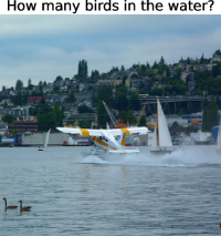
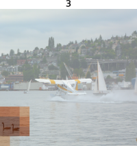
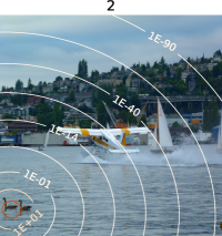
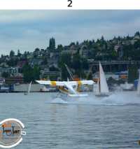
Figure 5: Attention maps for an example in VQA-v2: original image, discrete attention, continuous softmax, and continuous sparsemax.

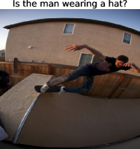
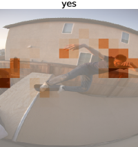
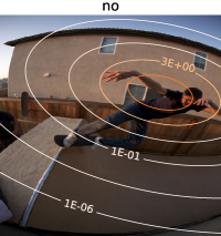
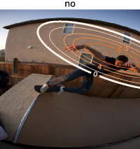
Figure 6: Attention maps for an example in VQA-v2: original image, discrete attention, continuous softmax, and continuous sparsemax.

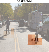
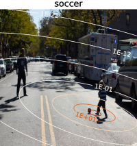
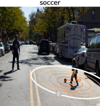
Figure 7: Attention maps for an example in VQA-v2: original image, discrete attention, continuous softmax, and continuous sparsemax.

References

• Brown [1986] Lawrence D Brown. Fundamentals of Statistical Exponential Families with Applications in Statistical Decision Theory. Institute of Mathematical Statistics, 1986.
• Barndorff-Nielsen [2014] Ole Barndorff-Nielsen. Information and Exponential Families in Statistical Theory. John Wiley & Sons, 2014.
• Pitman [1936] Edwin James George Pitman. Sufficient statistics and intrinsic accuracy. In Mathematical Proceedings of the Cambridge Philosophical Society, volume 32, pages 567–579. Cambridge University Press, 1936.
• Darmois [1935] Georges Darmois. Sur les lois de probabilitéa estimation exhaustive. CR Acad. Sci. Paris, 260(1265):85, 1935.
• Koopman [1936] Bernard Osgood Koopman. On distributions admitting a sufficient statistic. Transactions of the American Mathematical society, 39(3):399–409, 1936.
• Martins and Astudillo [2016] André FT Martins and Ramón Fernandez Astudillo. From softmax to sparsemax: A sparse model of attention and multi-label classification. In Proc. of ICML, 2016.
• Blondel et al. [2020] Mathieu Blondel, André FT Martins, and Vlad Niculae. Learning with fenchel-young losses. Journal of Machine Learning Research, 21(35):1–69, 2020.
• Peters et al. [2019] Ben Peters, Vlad Niculae, and André F.T. Martins. Sparse sequence-to-sequence models. In Proc. of ACL, 2019.
• Correia et al. [2019] Gonçalo M Correia, Vlad Niculae, and André FT Martins. Adaptively sparse transformers. In Proceedings of the 2019 Conference on Empirical Methods in Natural Language Processing and the 9th International Joint Conference on Natural Language Processing (EMNLP-IJCNLP), pages 2174–2184, 2019.
• Naudts [2009] Jan Naudts. The q-exponential family in statistical physics. Central European Journal of Physics, 7(3):405–413, 2009.
• Sears [2008] Timothy Sears. Generalized Maximum Entropy, Convexity and Machine Learning. PhD thesis, The Australian National University, 2008.
• Ding and Vishwanathan [2010] Nan Ding and S.V.N. Vishwanathan. t-logistic regression. In J. D. Lafferty, C. K. I. Williams, J. Shawe-Taylor, R. S. Zemel, and A. Culotta, editors, Advances in Neural Information Processing Systems 23, pages 514–522. Curran Associates, Inc., 2010.
• Tsallis [1988] Constantino Tsallis. Possible generalization of Boltzmann-Gibbs statistics. Journal of Statistical Physics, 52:479–487, 1988.
• Bahdanau et al. [2015] Dzmitry Bahdanau, Kyunghyun Cho, and Yoshua Bengio. Neural machine translation by jointly learning to align and translate. In Proc. of ICLR, 2015.
• Halmos [2013] Paul R Halmos. Measure Theory, volume 18. Springer, 2013.
• Bridle [1990] John S. Bridle. Probabilistic interpretation of feedforward classification network outputs, with relationships to statistical pattern recognition. In Françoise Fogelman-Soulié and Jeanny Hérault, editors, Neurocomputing, pages 227–236. Springer, 1990.
• Cover and Thomas [2012] Thomas M Cover and Joy A Thomas. Elements of Information Theory. John Wiley & Sons, 2012.
• Amari [2016] Shun-ichi Amari. Information geometry and its applications, volume 194. Springer, 2016.
• Havrda and Charvát [1967] Jan Havrda and František Charvát. Quantification method of classification processes. concept of structural $a$-entropy. Kybernetika, 3(1):30–35, 1967.
• Jost [2006] L. Jost. Entropy and diversity. Oikos, 113:363––375, 2006.
• Rao [1982] R.A. Rao. Gini-Simpson index of diversity: a characterization, generalization, and applications. Utilitas Mathematics, 21:273–282, 1982.
• Figueiredo [2001] M. Figueiredo. Adaptive sparseness using Jeffreys prior. In Proc. of NeurIPS, pages 697–704, 2001.
• Tipping [2001] M. Tipping. Sparse Bayesian learning and the relevance vector machine. Journal of Machine Learning Research, 1:211–244, 2001.
• Matsuzoe and Ohara [2012] Hiroshi Matsuzoe and Atsumi Ohara. Geometry for q-exponential families. In Recent Progress in Differential Geometry and its Related Fields, pages 55–71. World Scientific, 2012.
• Amari and Ohara [2011] Shun-ichi Amari and Atsumi Ohara. Geometry of q-exponential family of probability distributions. Entropy, 13(6):1170–1185, 2011.
• Epanechnikov [1969] Vassiliy A Epanechnikov. Non-parametric estimation of a multivariate probability density. Theory of Probability & Its Applications, 14(1):153–158, 1969.
• Sukhbaatar et al. [2015] Sainbayar Sukhbaatar, Jason Weston, Rob Fergus, et al. End-to-end memory networks. In Advances in Neural Information Processing Systems, pages 2440–2448, 2015.
• Vaswani et al. [2017] Ashish Vaswani, Noam Shazeer, Niki Parmar, Jakob Uszkoreit, Llion Jones, Aidan N Gomez, Łukasz Kaiser, and Illia Polosukhin. Attention is all you need. In Proc. of NeurIPS, 2017.
• Maas et al. [2011] Andrew L Maas, Raymond E Daly, Peter T Pham, Dan Huang, Andrew Y Ng, and Christopher Potts. Learning word vectors for sentiment analysis. In Proc. of NAACL-HLT, 2011.
• Cettolo et al. [2017] Mauro Cettolo, Marcello Federico, Luisa Bentivogli, Niehues Jan, Stüker Sebastian, Sudoh Katsuitho, Yoshino Koichiro, and Federmann Christian. Overview of the IWSLT 2017 evaluation campaign. In Proc. of IWSLT, pages 2–14, 2017.
• Goyal et al. [2019] Yash Goyal, Tejas Khot, Aishwarya Agrawal, Douglas Summers-Stay, Dhruv Batra, and Devi Parikh. Making the V in VQA Matter: Elevating the Role of Image Understanding in Visual Question Answering. International Journal of Computer Vision, 127(4):398–414, 2019.
• Yu et al. [2019] Zhou Yu, Jun Yu, Yuhao Cui, Dacheng Tao, and Qi Tian. Deep modular co-attention networks for visual question answering. Proceedings of the IEEE Computer Society Conference on Computer Vision and Pattern Recognition, pages 6274–6283, 2019.
• Anderson et al. [2018a] Peter Anderson, Xiaodong He, Chris Buehler, Damien Teney, Mark Johnson, Stephen Gould, and Lei Zhang. Bottom-up and top-down attention for image captioning and visual question answering. In Proceedings of the IEEE conference on computer vision and pattern recognition, pages 6077–6086, 2018a.
• Wang et al. [2018] Shenlong Wang, Simon Suo, Wei-Chiu Ma, Andrei Pokrovsky, and Raquel Urtasun. Deep parametric continuous convolutional neural networks. In Proceedings of the IEEE Conference on Computer Vision and Pattern Recognition, pages 2589–2597, 2018.
• Schütt et al. [2017] Kristof Schütt, Pieter-Jan Kindermans, Huziel Enoc Sauceda Felix, Stefan Chmiela, Alexandre Tkatchenko, and Klaus-Robert Müller. Schnet: A continuous-filter convolutional neural network for modeling quantum interactions. In Advances in neural information processing systems, pages 991–1001, 2017.
• Funahashi and Nakamura [1993] Ken-ichi Funahashi and Yuichi Nakamura. Approximation of dynamical systems by continuous time recurrent neural networks. Neural networks, 6(6):801–806, 1993.
• Rubanova et al. [2019] Yulia Rubanova, Tian Qi Chen, and David K Duvenaud. Latent ordinary differential equations for irregularly-sampled time series. In Advances in Neural Information Processing Systems, pages 5321–5331, 2019.
• Chen et al. [2018] Tian Qi Chen, Yulia Rubanova, Jesse Bettencourt, and David K Duvenaud. Neural ordinary differential equations. In Advances in neural information processing systems, pages 6571–6583, 2018.
• Kumar and Tsvetkov [2018] Sachin Kumar and Yulia Tsvetkov. Von mises-fisher loss for training sequence to sequence models with continuous outputs. In Proc. of ICLR, 2018.
• Cordonnier et al. [2019] Jean-Baptiste Cordonnier, Andreas Loukas, and Martin Jaggi. On the relationship between self-attention and convolutional layers. In International Conference on Learning Representations, 2019.
• You et al. [2020] Weiqiu You, Simeng Sun, and Mohit Iyyer. Hard-coded Gaussian attention for neural machine translation. In Proceedings of the 58th Annual Meeting of the Association for Computational Linguistics, pages 7689–7700, Online, July 2020. Association for Computational Linguistics. doi: 10.18653/v1/2020.acl-main.687. URL https://www.aclweb.org/anthology/2020.acl-main.687.
• Gregor et al. [2015] Karol Gregor, Ivo Danihelka, Alex Graves, Danilo Rezende, and Daan Wierstra. Draw: A recurrent neural network for image generation. In International Conference on Machine Learning, pages 1462–1471, 2015.
• Jain and Wallace [2019] Sarthak Jain and Byron C Wallace. Attention is not explanation. In Proc. NAACL-HLT, 2019.
• Serrano and Smith [2019] Sofia Serrano and Noah A Smith. Is attention interpretable? In Proc. ACL, 2019.
• Wiegreffe and Pinter [2019] Sarah Wiegreffe and Yuval Pinter. Attention is not not explanation. In Proc. EMNLP-IJCNLP, 2019.
• Wang et al. [2019] Tianlu Wang, Jieyu Zhao, Mark Yatskar, Kai-Wei Chang, and Vicente Ordonez. Balanced datasets are not enough: Estimating and mitigating gender bias in deep image representations. In Proceedings of the IEEE International Conference on Computer Vision, pages 5310–5319, 2019.
• Strubell et al. [2019] Emma Strubell, Ananya Ganesh, and Andrew McCallum. Energy and policy considerations for deep learning in nlp. In Proceedings of the 57th Annual Meeting of the Association for Computational Linguistics, pages 3645–3650, 2019.
• Bauschke and Combettes [2011] Heinz Bauschke and Patrick Combettes. Convex Analysis and Monotone Operator Theory in Hilbert Spaces. Springer, 2011.
• Bregman [1967] Lev M Bregman. The relaxation method of finding the common point of convex sets and its application to the solution of problems in convex programming. USSR Computational Mathematics and Mathematical Physics, 7(3):200–217, 1967.
• Abe [2003] Sumiyoshi Abe. Geometry of escort distributions. Physical Review E, 68(3):031101, 2003.
• Jaynes [1957] Edwin T Jaynes. Information theory and statistical mechanics. Physical review, 106(4):620, 1957.
• Sennrich et al. [2016] Rico Sennrich, Barry Haddow, and Alexandra Birch. Neural machine translation of rare words with subword units. In Proc. of ACL, 2016.
• Kreutzer et al. [2019] Julia Kreutzer, Joost Bastings, and Stefan Riezler. Joey nmt: A minimalist nmt toolkit for novices. In Proc. of EMNLP-IJCNLP: System Demonstrations, pages 109–114, 2019.
• He et al. [2016] Kaiming He, Xiangyu Zhang, Shaoqing Ren, and Jian Sun. Deep residual learning for image recognition. Proceedings of the IEEE Computer Society Conference on Computer Vision and Pattern Recognition, 2016-Decem:770–778, 2016.
• Russakovsky et al. [2015] Olga Russakovsky, Jia Deng, Hao Su, Jonathan Krause, Sanjeev Satheesh, Sean Ma, Zhiheng Huang, Andrej Karpathy, Aditya Khosla, Michael Bernstein, Alexander C. Berg, and Li Fei-Fei. ImageNet Large Scale Visual Recognition Challenge. International Journal of Computer Vision, 115(3):211–252, 2015.
• Anderson et al. [2018b] Peter Anderson, Xiaodong He, Chris Buehler, Damien Teney, Mark Johnson, Stephen Gould, and Lei Zhang. Bottom-Up and Top-Down Attention for Image Captioning and Visual Question Answering. Proceedings of the IEEE Computer Society Conference on Computer Vision and Pattern Recognition, pages 6077–6086, 2018b.
• Pennington et al. [2014] Jeffrey Pennington, Richard Socher, and Christopher D. Manning. Glove: Global vectors for word representation. In Proc. of EMNLP, pages 1532–1543, 2014.