Deep Reinforcement and InfoMax Learning

Abstract

We begin with the hypothesis that a model-free agent whose representations are predictive of properties of future states (beyond expected rewards) will be more capable of solving and adapting to new RL problems. To test that hypothesis, we introduce an objective based on Deep InfoMax (DIM) which trains the agent to predict the future by maximizing the mutual information between its internal representation of successive timesteps. We test our approach in several synthetic settings, where it successfully learns representations that are predictive of the future. Finally, we augment C51, a strong RL baseline, with our temporal DIM objective and demonstrate improved performance on a continual learning task and on the recently introduced Procgen environment.

1 Introduction

In reinforcement learning (RL), model-based agents are characterized by their ability to predict future states and rewards based on past states and actions [Sutton and Barto, 1998, Ha and Schmidhuber, 2018, Hafner et al., 2019a]. Model-based methods can be seen through the representation learning [Goodfellow et al., 2017] lens as endowing the agent with internal representations that are predictive of the future conditioned on its actions. This ultimately gives the agent means to plan – by e.g. considering a distribution of possible future trajectories and picking the best course of action.

In contrast, model-free methods do not explicitly model the environment, and instead learn a policy that maximizes reward or a function that estimates the optimal values of states and actions [Mnih et al., 2015, Schulman et al., 2017, Pong et al., 2018]. They can use large amounts of training data and excel in high-dimensional state and action spaces. However, this is mostly true for fixed reward functions; despite success on many benchmarks, model-free agents typically generalize poorly when the environment or reward function changes [Farebrother et al., 2018, Tachet des Combes et al., 2018] and can have high sample complexity.

Viewing model-based agents from a representation learning perspective, a desired outcome is an agent that understands the underlying generative factors of the environment that determine the observed state/action sequences, leading to generalization to other environments built from the same generative factors. In addition, learning a predictive model affords a richer learning signal than those provided by reward alone, which could reduce sample complexity compared to model-free methods.

Our work is based on the hypothesis that a model-free agent whose representations are predictive of properties of future states (beyond expected rewards) will be more capable of solving and adapting to new RL problems and, in a way, incorporate aspects of model-based learning. To learn representations with model-like properties, we consider a self-supervised objective derived from variants of Deep InfoMax [DIM, Hjelm et al., 2018, Bachman et al., 2019, Anand et al., 2019]. We expect this type of contrastive estimation [Hyvarinen and Morioka, 2016] will give the agent a better understanding of the underlying factors of the environment and how they relate to its actions, eventually leading to better performance in transfer and lifelong learning problems. We examine the properties of the learnt representations in simple domains such as disjoint and glued Markov chains, and more complex environments such as a 2d Ising model, a sequential variant of Ms. PacMan from the Atari Learning Environment [ALE, Bellemare et al., 2013], and all 16 games from the Procgen suite [Cobbe et al., 2019]. Our contributions are as follows:

• We propose a simple auxiliary objective that maximizes concordance between representations of successive states, given the action. We also introduce a simple adaptive mechanism that adjusts the time-scales of the contrastive tasks based on the likelihood of subsequent actions under the current RL policy.

• We present a series of experiments showing how our objective can be used as a measure of similarity and predictability, and how it behaves in partially deterministic systems.

• Finally, we show that augmenting a standard RL agent with our contrastive objective can i) lead to faster adaptation in a continual learning setting, and ii) improve overall performance on the Procgen suite.

2 Background

Just as humans are able to retain old skills when taught new ones [Wixted, 2004], we strive for RL agents that are able to adapt quickly and reuse knowledge when presented a sequence of different tasks with variable reward functions. The reason for this is that real-world applications or downstream tasks can be difficult to anticipate before deployment, particularly with complex environments involving other intelligent agents such as humans. Unfortunately, this proves to be very challenging even for state-of-the-art systems [Atkinson et al., 2018], leading to complex deployment scenarios.

Continual Learning (CL) is a learning framework meant to benchmark an agent’s ability to adapt to new tasks by using auxiliary information about the relatedness across tasks and timescales [Kaplanis et al., 2018, Mankowitz et al., 2018, Doan et al., 2020]. Meta-learning [Thrun and Pratt, 1998, Finn et al., 2017] and multi-task learning [Hessel et al., 2019, D’Eramo et al., 2019] have shown good performance in CL by explicitly training the agent to transfer well between tasks.

In this study, we focus on the following inductive bias: while the reward function may change or vary, the underlying environment dynamics typically do not change as much. To test if that inductive bias is useful, we use auxiliary loss functions to encourage the agent to learn about the underlying generative factors and their associated dynamics in the environment, which can result in better sample efficiency and transfer capabilities (compared to learning from rewards only). Previous work has shown this idea to be useful when training RL agents: e.g., Jaderberg et al. [2016] train the agent to predict future states given the current state-action pair, while Mohamed and Rezende [2015] uses empowerment to measure concordance between a sequence of future actions and the end state. Recent work such as DeepMDP [Gelada et al., 2019] uses a latent variable model to represent transition and reward functions in a high-dimensional abstract space. In model-based RL, various agents, such as PlaNet [Hafner et al., 2019b], Dreamer [Hafner et al., 2019a], or MuZero [Schrittwieser et al., 2019], have also shown strong asymptotic performance.

Contrastive representation learning methods are based on training an encoder to capture information that is shared across different views of the data in the features it produces for each input. The similar (i.e. positive) examples are typically either taken from different “locations” of the data [e.g., spatial patches or temporal locations, see Hjelm et al., 2018, Oord et al., 2018, Anand et al., 2019, Hénaff et al., 2019] or obtained through data augmentation [Wu et al., 2018, He et al., 2019, Bachman et al., 2019, Tian et al., 2019, Chen et al., 2020]. Contrastive models rely on a variety of objectives to encourage similarity between features. Typically, a scoring function [e.g., dot product or cosine similarity between pairs of features, see Wu et al., 2018] that lower-bounds mutual information is maximized [Belghazi et al., 2018, Hjelm et al., 2018, Oord et al., 2018, Poole et al., 2019].

A number of works have applied the above ideas to RL settings. Contrastive Predictive Coding [CPC, Oord et al., 2018] augments an A2C agent with an autoregressive contrastive task across a sequence of frames, improving performance on 5 DeepMind lab games [Beattie et al., 2016]. EMI [Kim et al., 2019] uses a Jensen-Shannon divergence-based lower bound on mutual information across subsequent frames as an exploration bonus. CURL [Srinivas et al., 2020] uses a contrastive task using augmented versions of the same frame (does not use future frames) as an auxiliary task to an RL algorithm. Finally, HOMER [Misra et al., 2019] produces a policy cover for block MDPs by learning backward and forward state abstractions using contrastive learning objectives. It is worth noting that HOMER has statistical guarantees for its performance on certain hard exploration problems.

Our work, DRIML, predicts future states conditioned on the current state-action pair at multiple scales, drawing upon ideas encapsulated in Augmented Multiscale Deep InfoMax [AMDIM, Bachman et al., 2019] and Spatio-Temporal DIM [ST-DIM, Anand et al., 2019]. Our method is flexible w.r.t. these tasks: we can employ the DIM tasks over features that constitute the full frame (global) or that are specific to local patches (local) or both. It is also robust w.r.t. time-scales of the contrastive tasks, though we show that adapting this time scale according to the predictability of subsequent actions under the current RL policy improves performance substantially.

3 Preliminaries

We assume the usual Markov Decision Process (MDP) setting (see Appendix for details), with the MDP denoted as $\mathcal{M}$, states as $s$, actions as $a$, and the policy as $\pi$. Since we focus on exploring the role of auxiliary losses in continuous learning, we use C51 [Bellemare et al., 2017], which extends DQN [Mnih et al., 2015] to predict the full distribution of potential future rewards, for training the agent due to its strong performance on control tasks from pixels. C51 minimizes the following loss:

$$\mathcal{L}_{RL}=D_{KL}(\lfloor\mathcal{T}Z(s,a)\rfloor_{51}||Z(s,a)),$$ (1)

where $D_{KL}$ is the Kullback-Leibler divergence, $Z(s,a)$ is the distribution of future discounted returns under the current policy ($\mathbb{E}[Z(s,a)]=Q(s,a)$), $\mathcal{T}$ is the distributional Bellman operator [Bellemare et al., 2019] and $\lfloor\cdot\rfloor_{51}$ is an operator which projects $Z$ onto a fixed support of $51$.

3.1 State-action mutual information maximization

Mutual information (MI) measures the amount of information shared between a pair of random variables and can be estimated using neural networks [Belghazi et al., 2018]. Recent representation learning algorithms [Oord et al., 2018, Hjelm et al., 2018, Tian et al., 2019, He et al., 2019] train encoders to maximize the MI between features taken from different views of the input – e.g., different patches in an image, different timesteps in a sequence, or different versions of an image produced by applying data augmentation to it.

Let $k$ be some fixed temporal offset. Running a policy $\pi$ in the MDP $\mathcal{M}$ generates a distribution over tuples $(s_{t},a_{t},s_{t+k})$, where $s_{t}$ corresponds to the state of $\mathcal{M}$ at some timestep $t$, $a_{t}$ to the action selected by $\pi$ in state $s_{t}$ and $s_{t+k}$ to the state of $\mathcal{M}$ at timestep $t+k$, reached by following $\pi$. $S_{t}$, $A_{t}$ and $S_{t+k}$ stand for the corresponding random variables. We also denote the joint distribution of these variables, as well as their associated marginals, using $p$. We are interested in learning representations of state-action pairs that have high MI with the representation of states later in the trajectory. The MI between e.g. state-action pairs $(S_{t},A_{t})$ and their future states $S_{t+k}$ is defined as follows:

$$\mathcal{I}([S_{t},A_{t}],S_{t+k};\pi)=\mathbb{E}_{p_{\pi}(s_{t},a_{t},s_{t+k})}\bigg{[}\log\frac{p_{\pi}(s_{t},a_{t},s_{t+k})}{p_{\pi}(s_{t},a_{t})p_{\pi}(s_{t+k})}\bigg{]},$$ (2)

where $p_{\pi}$ denotes distributions under $\pi$. Estimating the MI can be done by training a classifier that discriminates between a sample drawn from the joint distribution – the numerator of Eq. 2 – and a sample from the product of marginals – its denominator. A sample from the product of marginals is usually obtained by replacing $s_{t+k}$ (positive sample) with a state picked at random from another trajectory (negative sample). Letting $S^{-}$ denote a set of such negative samples, the infoNCE loss function [Gutmann and Hyvärinen, 2010, Oord et al., 2018] that we use to maximize a lower bound on the MI in Eq. 2 (with the added encoders for the states and actions) takes the following form:

$$\mathcal{L}_{NCE}:=-\mathbb{E}_{p_{\pi}(s_{t},a_{t},s_{t+k})}\mathbb{E}_{S^{-}}\bigg{[}\log\frac{\exp(\phi(\Psi(s_{t},a_{t}),\Phi(s_{t+k})))}{\sum_{s^{\prime}\in S^{-}\cup\{s_{t+k}\}}\exp(\phi(\Psi(s_{t},a_{t}),\Phi(s^{\prime})))}\bigg{]},$$ (3)

where $\Psi(s,a),\Phi(s)$ are features that depend on state-action pairs and states, respectively, and $\phi$ is a function that outputs a scalar-valued score. Minimizing $\mathcal{L}_{NCE}$ with respect to $\Phi,\Psi$, and $\phi$ maximizes the MI between these features. In practice, we construct $S^{-}$ by including all states $\tilde{s}_{t+k}$ from other tuples $(\tilde{s}_{t},\tilde{a}_{t},\tilde{s}_{t+k})$ in the same minibatch as the relevant $(s_{t},a_{t},s_{t+k})$. I.e., for a batch containing $N$ tuples $(s_{t},a_{t},s_{t+k})$, each $S^{-}$ would contain $N-1$ negative samples.

4 Architecture and Algorithm

We now specify forms for the functions $\Phi,\Psi$, and $\phi$. We consider a deep neural network $\Theta:\mathcal{S}\to\prod_{i=1}^{5}\mathcal{F}_{i}$ which maps input states onto a sequence of progressively more “global” (or less “local”) feature spaces. In practice, $\Theta$ is a CNN composed of functions that sequentially map inputs to features $\{f_{i}\in\mathcal{F}_{i}\}_{1\leq i\leq 5}$ (lower to upper “levels” of the network). For ease of explanation, we formulate our model using specific features (e.g., local features $f_{3}$ and global features $f_{4}$), but our model covers any set of features extracted from $\Theta$ used for the objective below as well as other choices for $\Theta$.

The features ${f_{5}}$ are the output of the network’s last layer and correspond to the standard C51 value heads (i.e., they span a space of 51 atoms per action) . For the auxiliary objective, we follow a variant of Deep InfoMax [DIM, Hjelm et al., 2018, Anand et al., 2019, Bachman et al., 2019], and train the encoder to maximize the mutual information (MI) between local and global “views” of tuples $(s_{t},a_{t},s_{t+k})$. The local and global views are realized by selecting $f_{3}\in\mathcal{F}_{3}$ and $f_{4}\in\mathcal{F}_{4}$ respectively. In order to simultaneously estimate and maximize the MI, we embed the action (represented as a one-hot vector) using a function $\Psi_{a}:\mathcal{A}\to\tilde{\mathcal{A}}$. We then map the local states $f_{3}$ and the embedded action using a function $\Psi_{3}:\mathcal{F}_{3}\times\tilde{\mathcal{A}}\to L$, and do the same with the global states $f_{4}$, i.e., $\Psi_{4}:\mathcal{F}_{4}\times\tilde{\mathcal{A}}\to G$. In addition, we have two more functions, $\Phi_{3}:\mathcal{F}_{3}\to L$ and $\Phi_{4}:\mathcal{F}_{4}\to G$ that map features without the actions, which will be applied to features from “future” timesteps. Note that $L$ can be thought of as a product of local spaces (corresponding to different patches in the input, or equivalently different receptive fields), each with the same dimensionality as $G$.

We use the outputs of these functions to produce a scalar-valued score between any combination of local and global representations of state $s_{t}$ and $s_{t+k}$, conditioned on action $a_{t}$:

$$\phi_{NtM}(s_{t},a,s_{t+k}) :=\Psi_{N}(f_{N}(s_{t}),\Psi_{a}(a_{t}))^{\top}\Phi_{M}(f_{M}(s_{t+k})),\;M,N\in\{3,4\}.$$ (4)

In practice, for the functions that take features and actions as input, we simply concatenate the values at position $f_{3}$ (local) or $f_{4}$ (global) with the embedded action $\Psi_{a}(a)$, and feed the resulting tensor into the appropriate function $\Psi_{3}$ or $\Psi_{4}$. All functions that process global and local features are computed using $1\times 1$ convolutions. See Figure 1 for a visual representation of our model.

We use the scores from Eq. 4 when computing the infoNCE loss [Oord et al., 2018] for our objective, using $(s_{t},a_{t},s_{t+k})$ tuples sampled from trajectories stored in an experience replay buffer:

$$\mathcal{L}_{DIM}^{NtM}:=-\mathbb{E}_{p_{\pi}(s_{t},a_{t},s_{t+k})}\mathbb{E}_{S^{-}}\bigg{[}\log\frac{\exp(\phi_{NtM}(s_{t},a_{t},s_{t+k}))}{\sum_{s^{\prime}\in S^{-}\cup\{s_{t+k}\}}\exp(\phi_{NtM}(s_{t},a_{t},s^{\prime}))}\bigg{]}\;.$$ (5)

Combining Eq. 5 with the RL update in Eq. 1 yields our full training objective, which we call DRIML . We optimize $\Theta,\Psi_{3,4,a}$, and $\Phi_{3,4}$ jointly using a single loss function:

$$\mathcal{L}_{DRIML}=\mathcal{L}_{RL}+\sum_{M,N\in\{3,4\}}\lambda_{NtM}\mathcal{L}^{NtM}_{DIM}$$ (6)

Note that, in practice, the compute cost which Eq. 6 adds to the core RL algorithm is minimal, since it only requires additional passes through the (small) state/action embedding functions followed by an outer product.

Input : Batch $\mathcal{B}$ sampled from the replay buffer, $\{\lambda_{NtM}\}_{N,M\in\{3,4\}}$, strictly positive integer $k$

Update $\Theta$ using Eq. 1;

$s,a,s^{\prime},x\leftarrow\mathcal{B}[s_{t}],\mathcal{B}[a_{t}],\mathcal{B}[s_{t+k}],\mathcal{B}[s_{t^{\prime}\neq t+k}]$;

for N in $\{$3,4$\}$ do

       for M in $\{$3,4$\}$ do

             if $\lambda_{NtM}>0$ then

                   Compute $\mathcal{L}_{DIM}^{NtM}$ using Eq. 5 (see Appendix 8.5 for PyTorch code);

                   Update $\Theta,\Psi_{3,4,a}$, and $\Phi_{3,4}$ using gradients of $\lambda_{NtM}\mathcal{L}_{DIM}^{NtM}$;

                  

             end if

            

       end for

      

end for

Algorithm 1 Deep Reinforcement and InfoMax Learning (DRIML)

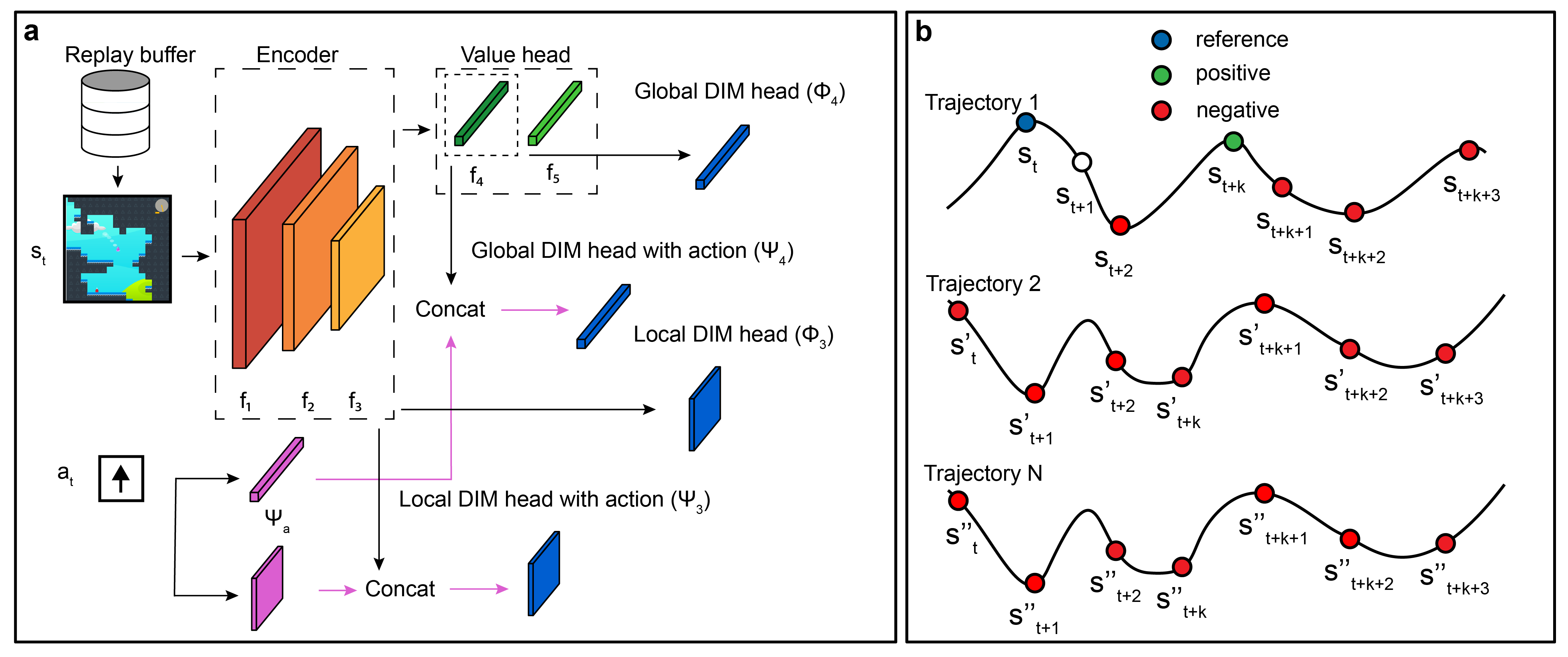
Figure 1: (a) Example model architecture used for the encoder used for the RL and DIM objectives and (b) distribution of reference, positive and negative samples within training batch $\mathcal{B}$. Note that in our experiments, we either use only the local head, only the global head, or both.

The proposed Algorithm 1 introduces an auxiliary loss which improves predictive capabilities of value-based agents by boosting similarity of representations close in time.

5 Finding the Best Task Timescale

The above DRIML algorithm fixes the temporal offset for the contrastive task, $k$, which needs to be chosen a-priori. However, different games are based on MDPs whose dynamics operate at different timescales, which in turn means that the difficulty of predictive tasks across different games will vary at different scales. We could predict simultaneously at multiple timescales [as in Oord et al., 2018], yet this introduces additional complexity that could be overcome by simply finding the right timescale. In order to ensure our auxiliary loss learns useful insights about the underlying MDP, as well as make DRIML more generally useful across environments, we adapt the temporal offset $k$ automatically based on the distribution of the agent’s actions.

We propose to select an adaptive, game-specific look-ahead value $k$, by learning a function $q_{\pi}(a_{i},a_{j})$ which measures the log-odds of taking action $a_{j}$ after taking action $a_{i}$ when following policy $\pi$ in the environment (i.e. $p_{\pi}(A_{t+1}=a_{j}|A_{t}=a_{i})/p_{\pi}(A_{t+1}=a_{j})$). The values $q_{\pi}(a_{i},a_{j})$ are then used to sample a look-ahead value $k\in\{1,..,H\}$ from a non-homogeneous geometric (NHG) distribution. This particular choice of distribution was motivated by two desirable properties of NHG: (a) any discrete positive random variable can be represented via NHG [Mandelbaum et al., 2007] and (b) the expectation of $X\sim NHG(q_{1},..,q_{H})$ obeys the rule $1/\max_{i}q_{i}\leq\mathbb{E}[X]\leq 1/\min_{i}q_{i}$. The intuition is that, if the state dynamics are regular, this should be reflected in the predictability of the future actions conditioned on prior actions. Our algorithm captures this through a matrix $\mathbf{A}$, whose $i$-th row is the softmax of $q_{\pi}(a_{i},\cdot)$. $q_{\pi}(a_{i},a_{j})$ is learned off-policy using the same data from the buffer as the main algorithm; it is updated at the same frequency as the main DRIML parameters and trained to approximate the relevant log odds. This modification is small in relation to the DRIML algorithm, but it substantially improves results in our experiments. The sampling of $k$ is done via Algorithm 2, and additional analysis of the adaptive temporal offset is provided in Figure 2.

Input : Tuple $(s_{t},a_{t},a_{t+1},...,a_{t+H})$, maximal horizon $H$, stochastic matrix $\mathbf{A}$ of size $\mathcal{A}\times\mathcal{A}$

Output : Lookahead value $k:1\leq k\leq H$

for $i$ in $1,...,H$ do

       $k\leftarrow i$; // Updating value of k

      

      $b\sim\text{Bernoulli}(\mathbf{A}_{a_{t+i-1},a_{t+i}})$;

      if $b==0$ then

             break;

       end if

      

end for

Algorithm 2 Adaptive lookahead selection

Figure 2 shows the impact of adaptively selecting $k$ using the NHG sampling method. For instance, (i) depending on the nature of the game, DRIML-ada tends to repeat movement actions in navigation games and repeatedly fire in shooting games, and (ii) the value of $k$ tends to converge to 1 for games like Bigfish and Plunder as training progresses, which hints to an exploration-exploitation like trade-off.

Since many Procgen games do not have special actions such as fire or diagonal moves, DRIML-ada considers the actual actions (15 of them) and the visible actions (at most 15 of them) together in the adaptive lookahead selection algorithm.

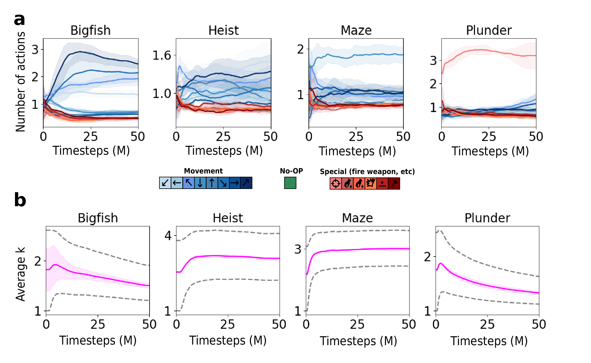
Figure 2: (a) Average number of movement, no-op and special actions taken by DRIML-ada on 4 Procgen games and (b) change in the average, max and min across batch values of $k$ as a function of training steps.

6 Experiments

In this section, we first show how our proposed objective can be used to estimate state similarity in single Markov chains. We then show that DRIML can capture dynamics in locally deterministic systems (Ising model), which is useful in domains with partially deterministic transitions. We then provide results on a continual version of the Ms. PacMan game where the DIM loss is shown to converge faster for more deterministic tasks, and to help in a continual learning setting. Finally, we provide results on Procgen [Cobbe et al., 2019], which show that DRIML performs well when trained on 500 levels with fixed order. All experimental details can be found in Appendix 8.6.

6.1 DRIML learns a transition ratio model

We first study the behaviour of DRIML’s loss on a simple Markov chain describing a biased random walk in $\{1,\cdots,K\}$. The bias is specified by a single parameter $\alpha$. The agent starting at state $i$ transitions to $i+1$ with probability $\alpha$ and to $i-1$ otherwise. The agent stays in states $1$ and $K$ with probability $1-\alpha$ and $\alpha$, respectively. We encode the current and next states (represented as one-hots) using a 1-hidden layer MLP (corresponding to $\Psi$ and $\Phi$ in equation 3), and then optimize the NCE loss $\mathcal{L}_{DIM}$ (the scoring function $\phi$ is also 1-hidden layer MLP, equation 3) to maximize the MI between representations of successive states. Results are shown in Fig. 3b, they are well aligned with the true transition matrix (Fig. 3c).

This toy experiment revealed an interesting observation: DRIML’s objective involves computing the ratio of the Markov transition operator over the stationary distribution, implying that the convergence rate is affected by the spectral gap of the average Markov transition operator, $\mathbf{T}^{\pi}_{ss^{\prime}}=\mathbb{E}_{a\sim\pi(s,\cdot)}[T(s,a,s^{\prime})]$ for transition operator $T$. That is, it depends on the difference between the two largest eigenvalues of $\mathbf{T}^{\pi}$, namely $1$ and $\lambda_{(2)}$. In the case of the random walk, the spectral gap of its transition matrix can be computed in closed-form as a function of $\alpha$. Its lowest value is reached in the neighbourhood $\alpha=0.5$, corresponding to the point where the system is least predictable (as shown by the mutual information, Fig 3c). However, since the matrix is not invertible for $\alpha=0.5$, we consider $\alpha=0.499$ instead. Derivations are available in Appendix 8.6.1, and more insights on the connection to the spectral gap are presented in Appendix 8.4.

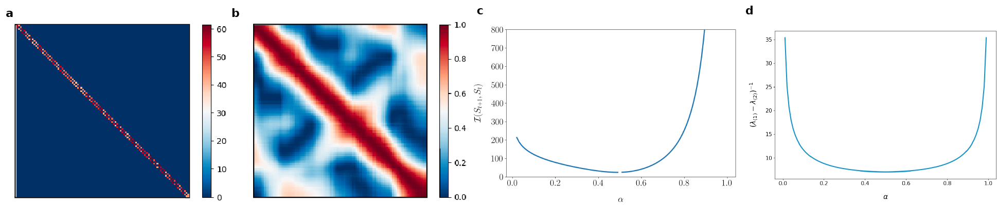
Figure 3: (a) Ratio of transition matrix over stationary vector for the random walk with $\alpha=0.499$, (b) the prediction matrix of being a pair of successive states learnt by $\mathcal{L}_{DIM}$, (c) the closed-form mutual information between consecutive states in time as a function of $\alpha$ (with simplified endpoint conditions) and (d) the true inverse spectral gap $(\lambda_{(1)}-\lambda_{(2)})^{-1}$ as a function of $\alpha$.

6.2 DRIML can capture complex partially deterministic dynamics

The goal of this experiment is to highlight the predictive capabilities of our DIM objective in a partially deterministic system. We consider a dynamical system composed of $N\times N$ pixels with values in $\{-1,1\}$, $S(t)=\{s_{ij}(t)\mid 1\leq i,j\leq N\}$. At the beginning of each episode, a patch corresponding to a quarter of the pixels is chosen at random in the grid. Pixels that do not belong to that patch evolve fully independently ($p(s_{ij}(t)=1\mid S(t-1))=p(s_{ij}(t)=1)=0.5$). Pixels from the patch obey a local dependence law, in the form of a standard Ising model: the value of a pixel at time $t$ only depends on the value of its neighbors at time $t-1$. This local dependence is obtained through a function $f$: $p(s_{ij}(t)|S(t-1))=f(\{s_{i^{\prime}j^{\prime}}(t-1)\mid|i-i^{\prime}|=|j-j^{\prime}|=1\})$ (see Appx 8.6.2 for details). Figure 4 shows the system at $t=32$ during three different episodes (black pixels correspond to values of $-1$, white to $1$). The patches are very distinct from the noise. We then train a convolutional encoder using our DIM objective on local “views” only (see Section 4).

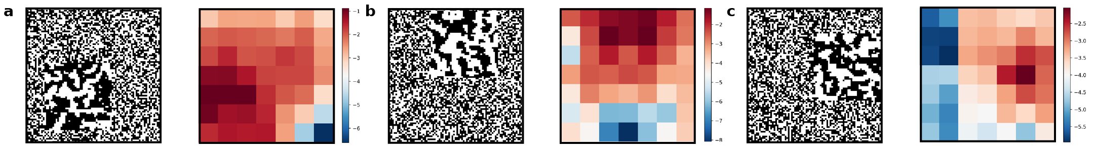
Figure 4: $42\times 42$ Ising model with temperature $\beta^{-1}=0.4$ overlaid onto a $84\times 84$ lattice of uniformly random spins $\{-1,+1\}$. The grayscale plots show each of the 3 systems at $t=32$; the color plots show the DIM similarity scores between $t=2$ and $t=3$.

Figure 4 shows the similarity scores between the local features of states at $t=2$ and the same features at $t=3$ (a local feature corresponds to a specific location in the convolutional maps). The heatmap regions containing the Ising model (larger-scale patterns) have higher scores than the noisy portions of the lattice. Local DIM is able to correctly encode regions of high temporal predictability.

6.3 A continual learning experiment on Ms. PacMan

We further complicate the task of the Ising model prediction by building on top of the Ms. PacMan game and introducing non-trivial dynamics. The environment is shown in the appendix.

In order to assess how well our auxiliary objective captures predictability in this MDP, we define its dynamics such that $\mathbb{P}[\text{Ghost}_{i}\text{ takes a random move}]=\varepsilon$. Intuitively, as $\varepsilon\to 1$, the enemies’ actions become less predictable, which in turn hinders the convergence rate of the contrastive loss. The four runs in Figure 5a correspond to various values of $\varepsilon$. We trained the agent using our $\mathcal{L}_{DRIML}$ objective. We can see that the convergence of the auxiliary loss becomes slower with growing $\varepsilon$, as the model struggles to predict $s_{t+1}$ given $(s_{t},a_{t})$. After 100k frames, the NCE objective allows to separate the four MDPs according to their principal source of randomness (red and blue curves). When $\varepsilon$ is close to 1, the auxiliary loss has a harder time finding features that predict the next state, and eventually ignores the random movements of enemies.

The second and more interesting setup we consider consists in making only one out of 4 enemies lethal, and changing which one every 5k episodes. Figure 5b shows that, as training progresses, the blue curve (C51) always reaches the same performance at the end of the 5k episodes, while DRIML’s steadily increases. The blue agent learns to ignore the harmless ghosts (they have no connection to the reward signal) and has to learn the task from scratch every time the lethal ghost changes. On the other hand, the DRIML agent (red curve) is incentivized to encode information about all the predictable objects on the screen (including the harmless ghosts), and as such adapts faster and faster to changes. Figure 5c shows the same PacMan environment with a quasi-deterministic Ising model evolving in the walled areas of the screen (details in appendix). For computational efficiency, we only run this experiment for 10k episodes. As before, DRIML outperforms C51 after the lethal ghost change, demonstrating that its representations encode more information about the dynamics of the environment (in particular about the harmless ghosts). The presence of additional distractors - the Ising model in the walls - did not impact that observation.

Figure 5: (a) average training NCE loss for various values of $\varepsilon$ as a function of timesteps, (b) average training reward with only one harmful enemy per level (dashed line indicates average terminal blue curve performance after each task) and (c) average training reward on PacMan + Ising noise in walled areas.

6.4 Performance on Procgen Benchmark

Finally, we demonstrate the beneficial impact of adding a DIM-like objective to C51 (DRIML) on the 500 first levels of all 16 Procgen tasks [Cobbe et al., 2019]. All algorithms are trained for 50M environment frames with the DQN [Mnih et al., 2015] architecture. The mean and standard deviation of the scores (over 3 seeds) are shown in Table 1; bold values indicate best performance.

Table 1: Average training returns collected after 50M of training frames, $\mathbin{\mbox{\unboldmath$\mathchar 8710\relax$}}$ one standard deviation.

Env	C51	CPC-1$\rightarrow$ 5	CURL	DRIML-noact	DRIML-randk	DRIML-fix	DRIML-ada
bigfish	$1.33\mathbin{\mbox{\unboldmath$\mathchar 8710\relax$}}0.12$	$1.17\mathbin{\mbox{\unboldmath$\mathchar 8710\relax$}}0.16$	$2.70\mathbin{\mbox{\unboldmath$\mathchar 8710\relax$}}1.30$	$1.19\mathbin{\mbox{\unboldmath$\mathchar 8710\relax$}}0.04$	$1.12\mathbin{\mbox{\unboldmath$\mathchar 8710\relax$}}1.03$	$2.02\mathbin{\mbox{\unboldmath$\mathchar 8710\relax$}}0.18$	4.45 $\mathbin{\mbox{\unboldmath$\mathchar 8710\relax$}}$ 0.71
bossfight	0.57$\mathbin{\mbox{\unboldmath$\mathchar 8710\relax$}}$0.05	0.52$\mathbin{\mbox{\unboldmath$\mathchar 8710\relax$}}$0.07	0.60$\mathbin{\mbox{\unboldmath$\mathchar 8710\relax$}}$0.06	0.47$\mathbin{\mbox{\unboldmath$\mathchar 8710\relax$}}$0.01	0.56$\mathbin{\mbox{\unboldmath$\mathchar 8710\relax$}}$0.03	0.67$\mathbin{\mbox{\unboldmath$\mathchar 8710\relax$}}$0.02	1.05$\mathbin{\mbox{\unboldmath$\mathchar 8710\relax$}}$0.19
caveflyer	9.19$\mathbin{\mbox{\unboldmath$\mathchar 8710\relax$}}$0.29	6.40$\mathbin{\mbox{\unboldmath$\mathchar 8710\relax$}}$0.56	6.94$\mathbin{\mbox{\unboldmath$\mathchar 8710\relax$}}$0.25	8.26$\mathbin{\mbox{\unboldmath$\mathchar 8710\relax$}}$0.26	7.92$\mathbin{\mbox{\unboldmath$\mathchar 8710\relax$}}$0.15	10.2$\mathbin{\mbox{\unboldmath$\mathchar 8710\relax$}}$0.41	6.77$\mathbin{\mbox{\unboldmath$\mathchar 8710\relax$}}$0.04
chaser	0.22$\mathbin{\mbox{\unboldmath$\mathchar 8710\relax$}}$0.04	0.21$\mathbin{\mbox{\unboldmath$\mathchar 8710\relax$}}$0.02	0.35$\mathbin{\mbox{\unboldmath$\mathchar 8710\relax$}}$0.04	0.23$\mathbin{\mbox{\unboldmath$\mathchar 8710\relax$}}$0.02	0.26$\mathbin{\mbox{\unboldmath$\mathchar 8710\relax$}}$0.01	0.29$\mathbin{\mbox{\unboldmath$\mathchar 8710\relax$}}$0.02	0.38$\mathbin{\mbox{\unboldmath$\mathchar 8710\relax$}}$0.04
climber	1.68$\mathbin{\mbox{\unboldmath$\mathchar 8710\relax$}}$0.10	1.71$\mathbin{\mbox{\unboldmath$\mathchar 8710\relax$}}$0.11	1.75$\mathbin{\mbox{\unboldmath$\mathchar 8710\relax$}}$0.09	1.57$\mathbin{\mbox{\unboldmath$\mathchar 8710\relax$}}$0.01	2.21$\mathbin{\mbox{\unboldmath$\mathchar 8710\relax$}}$0.48	2.26$\mathbin{\mbox{\unboldmath$\mathchar 8710\relax$}}$0.05	2.20$\mathbin{\mbox{\unboldmath$\mathchar 8710\relax$}}$0.08
coinrun	29.7$\mathbin{\mbox{\unboldmath$\mathchar 8710\relax$}}$5.44	11.4$\mathbin{\mbox{\unboldmath$\mathchar 8710\relax$}}$1.55	21.2$\mathbin{\mbox{\unboldmath$\mathchar 8710\relax$}}$1.94	13.2$\mathbin{\mbox{\unboldmath$\mathchar 8710\relax$}}$1.21	21.6$\mathbin{\mbox{\unboldmath$\mathchar 8710\relax$}}$1.97	27.2$\mathbin{\mbox{\unboldmath$\mathchar 8710\relax$}}$1.92	22.88$\mathbin{\mbox{\unboldmath$\mathchar 8710\relax$}}$0.4
dodgeball	1.20$\mathbin{\mbox{\unboldmath$\mathchar 8710\relax$}}$0.08	1.05$\mathbin{\mbox{\unboldmath$\mathchar 8710\relax$}}$0.04	1.09$\mathbin{\mbox{\unboldmath$\mathchar 8710\relax$}}$0.04	1.22$\mathbin{\mbox{\unboldmath$\mathchar 8710\relax$}}$0.04	1.19$\mathbin{\mbox{\unboldmath$\mathchar 8710\relax$}}$0.03	1.28$\mathbin{\mbox{\unboldmath$\mathchar 8710\relax$}}$0.02	1.44$\mathbin{\mbox{\unboldmath$\mathchar 8710\relax$}}$0.06
fruitbot	3.86$\mathbin{\mbox{\unboldmath$\mathchar 8710\relax$}}$0.96	4.56$\mathbin{\mbox{\unboldmath$\mathchar 8710\relax$}}$0.93	4.89$\mathbin{\mbox{\unboldmath$\mathchar 8710\relax$}}$0.71	5.42$\mathbin{\mbox{\unboldmath$\mathchar 8710\relax$}}$1.33	6.84$\mathbin{\mbox{\unboldmath$\mathchar 8710\relax$}}$0.24	5.40$\mathbin{\mbox{\unboldmath$\mathchar 8710\relax$}}$1.02	9.53$\mathbin{\mbox{\unboldmath$\mathchar 8710\relax$}}$0.29
heist	1.54$\mathbin{\mbox{\unboldmath$\mathchar 8710\relax$}}$0.10	0.93$\mathbin{\mbox{\unboldmath$\mathchar 8710\relax$}}$0.08	1.06$\mathbin{\mbox{\unboldmath$\mathchar 8710\relax$}}$0.05	1.04$\mathbin{\mbox{\unboldmath$\mathchar 8710\relax$}}$0.02	1.00$\mathbin{\mbox{\unboldmath$\mathchar 8710\relax$}}$0.05	1.30$\mathbin{\mbox{\unboldmath$\mathchar 8710\relax$}}$0.05	1.89$\mathbin{\mbox{\unboldmath$\mathchar 8710\relax$}}$0.02
jumper	13.2$\mathbin{\mbox{\unboldmath$\mathchar 8710\relax$}}$0.83	2.28$\mathbin{\mbox{\unboldmath$\mathchar 8710\relax$}}$0.44	10.3$\mathbin{\mbox{\unboldmath$\mathchar 8710\relax$}}$0.61	4.31$\mathbin{\mbox{\unboldmath$\mathchar 8710\relax$}}$0.64	5.62$\mathbin{\mbox{\unboldmath$\mathchar 8710\relax$}}$0.27	12.6$\mathbin{\mbox{\unboldmath$\mathchar 8710\relax$}}$0.64	12.2$\mathbin{\mbox{\unboldmath$\mathchar 8710\relax$}}$0.42
leaper	5.03$\mathbin{\mbox{\unboldmath$\mathchar 8710\relax$}}$0.14	4.01$\mathbin{\mbox{\unboldmath$\mathchar 8710\relax$}}$0.71	3.94$\mathbin{\mbox{\unboldmath$\mathchar 8710\relax$}}$0.46	5.40$\mathbin{\mbox{\unboldmath$\mathchar 8710\relax$}}$0.09	4.24$\mathbin{\mbox{\unboldmath$\mathchar 8710\relax$}}$1.17	6.17$\mathbin{\mbox{\unboldmath$\mathchar 8710\relax$}}$0.29	6.35$\mathbin{\mbox{\unboldmath$\mathchar 8710\relax$}}$0.46
maze	2.36$\mathbin{\mbox{\unboldmath$\mathchar 8710\relax$}}$0.09	1.14$\mathbin{\mbox{\unboldmath$\mathchar 8710\relax$}}$0.08	0.82$\mathbin{\mbox{\unboldmath$\mathchar 8710\relax$}}$0.20	1.44$\mathbin{\mbox{\unboldmath$\mathchar 8710\relax$}}$0.26	1.18$\mathbin{\mbox{\unboldmath$\mathchar 8710\relax$}}$0.03	1.38$\mathbin{\mbox{\unboldmath$\mathchar 8710\relax$}}$0.08	2.62$\mathbin{\mbox{\unboldmath$\mathchar 8710\relax$}}$0.10
miner	0.13$\mathbin{\mbox{\unboldmath$\mathchar 8710\relax$}}$0.01	0.13$\mathbin{\mbox{\unboldmath$\mathchar 8710\relax$}}$0.02	0.10$\mathbin{\mbox{\unboldmath$\mathchar 8710\relax$}}$0.01	0.12$\mathbin{\mbox{\unboldmath$\mathchar 8710\relax$}}$0.01	0.15$\mathbin{\mbox{\unboldmath$\mathchar 8710\relax$}}$0.01	0.14$\mathbin{\mbox{\unboldmath$\mathchar 8710\relax$}}$0.01	0.19$\mathbin{\mbox{\unboldmath$\mathchar 8710\relax$}}$0.02
ninja	9.36$\mathbin{\mbox{\unboldmath$\mathchar 8710\relax$}}$0.01	6.23$\mathbin{\mbox{\unboldmath$\mathchar 8710\relax$}}$0.82	5.84$\mathbin{\mbox{\unboldmath$\mathchar 8710\relax$}}$1.21	6.44$\mathbin{\mbox{\unboldmath$\mathchar 8710\relax$}}$0.22	8.13$\mathbin{\mbox{\unboldmath$\mathchar 8710\relax$}}$0.26	9.21$\mathbin{\mbox{\unboldmath$\mathchar 8710\relax$}}$0.25	8.74$\mathbin{\mbox{\unboldmath$\mathchar 8710\relax$}}$0.28
plunder	2.99$\mathbin{\mbox{\unboldmath$\mathchar 8710\relax$}}$0.07	3.00$\mathbin{\mbox{\unboldmath$\mathchar 8710\relax$}}$0.06	2.77$\mathbin{\mbox{\unboldmath$\mathchar 8710\relax$}}$0.14	3.20$\mathbin{\mbox{\unboldmath$\mathchar 8710\relax$}}$0.05	3.34$\mathbin{\mbox{\unboldmath$\mathchar 8710\relax$}}$0.09	3.37$\mathbin{\mbox{\unboldmath$\mathchar 8710\relax$}}$0.17	3.58$\mathbin{\mbox{\unboldmath$\mathchar 8710\relax$}}$0.04
starpilot	2.44$\mathbin{\mbox{\unboldmath$\mathchar 8710\relax$}}$0.12	2.87$\mathbin{\mbox{\unboldmath$\mathchar 8710\relax$}}$0.05	2.68$\mathbin{\mbox{\unboldmath$\mathchar 8710\relax$}}$0.09	3.70$\mathbin{\mbox{\unboldmath$\mathchar 8710\relax$}}$0.30	3.93$\mathbin{\mbox{\unboldmath$\mathchar 8710\relax$}}$0.04	4.56$\mathbin{\mbox{\unboldmath$\mathchar 8710\relax$}}$0.21	2.63$\mathbin{\mbox{\unboldmath$\mathchar 8710\relax$}}$0.16
Norm.score	$1.0$	$0.23$	$0.52$	$0.59$	$0.92$	$1.48$	$1.9$

Similarly to CURL, we used data augmentation on inputs to DRIML-fix to improve the model’s predictive capabilities in fast-paced environments (see App. 8.6.4). While we used the global-global loss in DRIML’s objective for all Procgen games, we have found that the local-local loss also had a beneficial effect on performance on a smaller set of games (e.g. starpilot, which has few moving entities on a dark background).

7 Discussion

In this paper, we introduced an auxiliary objective called Deep Reinforcement and InfoMax Learning (DRIML), which is based on maximizing concordance of state-action pairs with future states (at the representation level). We presented results showing that 1) DRIML implicitly learns a transition model by boosting state similarity, 2) it can improve performance of deep RL agents in a continual learning setting and 3) it boosts training performance in complex domains such as Procgen.

Broader Impact

This work proposes an auxiliary objective for model-free reinforcement learning agents. The objective shows improvements in a continual learning setting, as well as on average training rewards for a suite of complex video games. While the objective is developed in a visual setting, maximizing mutual information between features is a method that can be transported to other domains, such as text. Potential applications of deep reinforcement learning are (among others) healthcare, dialog systems, crop management, robotics, etc. Developing methods that are more robust to changes in the environment, and/or perform better in a continual learning setting can lead to improvements in those various applications. At the same time, our method fundamentally relies on deep learning tools and architectures, which are hard to interpret and prone to failures yet to be perfectly understood. Additionally, deep reinforcement learning also lacks formal performance guarantees, and so do deep reinforcement learning agents. Overall, it is essential to design failsafes when deploying such agents (including ours) in the real world.

8 Appendix

8.1 Markov Chains

Given a discrete state space $\mathcal{S}$ with probability measure $\mathbb{T}$, a discrete-time homogeneous Markov chain (MC) is a collection of random variables with the following property on its transition matrix $\mathbf{T}\in\mathbb{R}^{|\mathcal{S}|\times|\mathcal{S}|}$: $\mathbf{T}_{ss^{\prime}}=\mathbb{P}[S_{t+1}=s^{\prime}|S_{t}=s],\;\forall s,s^{\prime}\in\mathcal{S},\forall t\geq 0$. Assuming the Markov chain is ergodic, its invariant distribution $\bm{\rho}$ is the principal eigenvector of $\mathbf{T}$, which verifies $\bm{\rho}\mathbf{T}=\bm{\rho}$ and summarizes the long-term behaviour of the chain. We define the marginal distribution of $S_{t}$ as $p_{t}(s):=\mathbb{P}[S_{t}=s]=\mathbf{T}^{t}_{s:}$, and the initial distribution of $S$ as $p_{0}(s)$.

8.2 Markov Decision Processes

A discrete-time, finite-horizon Markov Decision Process [Bellman, 1957, Puterman, 2014, MDP] comprises a state space $\mathcal{S}$, an action space $\mathcal{A}$, a transition kernel $T:\mathcal{S}\times\mathcal{A}\times\mathcal{S}\mapsto[0,1]$, a reward function $r:\mathcal{S}\times\mathcal{A}\mapsto\mathbb{R}$ and a discount factor $\gamma\in[0,1]$. At every timestep $t$, an agent interacting with this MDP observes the current state $s_{t}\in\mathcal{S}$, selects an action $a_{t}\in\mathcal{A}$, and observes a reward $r(s_{t},a_{t})\in\mathbb{R}$ upon transitioning to a new state $s_{t+1}\sim T(s_{t},a_{t},\cdot)$. The goal of an agent in a discounted MDP is to learn a policy $\pi:\mathcal{S}\times\mathcal{A}\mapsto[0,1]$ such that taking actions $a_{t}\sim\pi(\cdot|s_{t})$ maximizes the expected sum of discounted returns,

$$V^{\pi}(s)=\mathbb{E}_{\pi}\bigg{[}\sum_{t=0}^{\infty}\gamma^{t}r(s_{t},a_{t})|s_{0}=s\bigg{]}.$$

To convert a MDP into a MC, one can let $\mathbf{T}^{\pi}_{ss^{\prime}}=\mathbb{E}_{a\sim\pi(s,\cdot)}[T(s,a,s^{\prime})]$, an operation which can be easily tensorized for computational efficiency in small state spaces [see Mazoure et al., 2020].

8.3 Link to invariant distribution

For a discrete state ergodic Markov chain specified by $\mathbf{P}$ and initial occupancy vector $\bm{p}_{0}$, its marginal state distribution at time $t$ is given by the Chapman-Kolmogorov form:

$$\mathbb{P}[S_{t}=s]=\bm{p}_{0}\mathbf{P}^{t}_{\cdot s},$$ (7)

and its limiting distribution $\bm{\sigma}$ is the infinite-time marginal

$$\lim_{t\to\infty}\mathbf{P}^{(t)}_{ss^{\prime}}=\bm{\sigma}_{s^{\prime}},\;s,s^{\prime}\in\mathcal{S}$$ (8)

which, if it exists, is exactly equal to the invariant distribution $\bm{\rho}$.

For the very restricted family of ergodic MDPs under fixed policy $\pi$, we can assume that $p_{t}$ converges to a time invariant distribution $\rho$.

Therefore,

$$\begin{split}\mathcal{I}_{t}(S,S^{\prime})&=\sum_{s^{\prime}\in\mathcal{S}}\sum_{s\in\mathcal{S}}p_{0}(\mathbf{P}^{t})_{:s}\mathbf{P}_{ss^{\prime}}\bigg{(}\log\mathbf{P}_{ss^{\prime}}-\log\{p_{0}(\mathbf{P}^{t+1})_{:s^{\prime}}\}\bigg{)}\\ \end{split}$$ (9)

Now, observe that $\mathcal{I}_{t}$ is closely linked to $T/\rho$ when samples come from timesteps close to $t_{mix}(\varepsilon)$. That is, interchanging swapping $\rho(s)$ and $p_{t}(s)$ at any state $s$ would yield at most $\delta(t)$ error. Moreover, existing results [Levin and Peres, 2017] from Markov chain theory provide bounds on $||(\mathbf{P}^{t+1})_{s:}-(\mathbf{P}^{t})_{s:}||_{TV}$ depending on the structure of the transition matrix.

If $\mathbf{P}$ has a limiting distribution $\bm{\sigma}$, then using the dominated convergence theorem allows to replace matrix powers by $\bm{\sigma}$, which is then replaced by the invariant distribution $\bm{\rho}$:

$$\begin{split}\lim_{t\to\infty}\mathcal{I}_{t}&=\sum_{s^{\prime}\in\mathcal{S}}\sum_{s\in\mathcal{S}}\bm{\rho}_{s}\bm{\rho}_{s^{\prime}}\bigg{(}\log\mathbf{P}_{ss^{\prime}}-\log\bm{\rho}_{s^{\prime}}\bigg{)}\\ &=\mathbb{E}_{\rho\times\rho}\bigg{(}\log\mathbf{P}_{ss^{\prime}}-\log\bm{\rho}_{s^{\prime}}\bigg{)}\end{split}$$ (10)

Of course, most real-life Markov decision processes do not actually have an invariant distribution since they have absorbing (or terminal) states. In this case, as the agent interacts with the environment, the DIM estimate of MI yields a rate of convergence which can be estimated based on the spectrum of $\mathbf{P}$.

Moreover, one could argue that since, in practice, we use off-policy algorithms for this sort of task, the gradient signal comes from various timesteps within the experience replay, which drives the model to learn features that are consistently predictive through time.

8.4 Predictability and Contrastive Learning

Information maximization has long been considered one of the standard principles for measuring correlation and performing feature selection [Song et al., 2012]. In the MDP context, high values of $\mathcal{I}([S_{t},A_{t}],S_{t+k})$ indicate that $(S_{t},A_{t})$ and $S_{t+k}$ have some form of dependence, while low values suggest independence. The fact that predictability (or more precisely determinism) in Markov systems is linked to the MI suggests a deeper connection to the spectrum of the transition kernel $T$. For instance, the set of eigenvalues of $T$ for a Markov decision process contains important information about the connectivity of said process, such as mixing time or number of densely connected clusters [Von Luxburg, 2007, Levin and Peres, 2017].

Consider the setting in which $\pi$ is fixed at some iteration in the optimization process. In the rest of this section, we let $\mathbf{T}$ denote the expected transition model $\mathbf{T}(s,s^{\prime})=\mathbb{E}_{\pi}[T(s,a,s^{\prime})]$ (it is a Markov chain). We let $\nu_{t}(s,s^{\prime})=\frac{\mathbf{T}(s,s^{\prime})}{p_{t+1}(s^{\prime})}$ be the ratio learnt when optimizing the infoNCE loss on samples drawn from the random variables $S_{t}$ and $S_{t+1}$ (for a fixed $t$) [Oord et al., 2018]. We also let $\nu_{\infty}(s,s^{\prime})=\frac{\mathbf{T}(s,s^{\prime})}{\bm{\rho}(s^{\prime})}$ be that ratio when the Markov chain has reached its stationary distribution $\bm{\rho}$ (see Section 8.1), and $\tilde{\nu}_{t}(s,s^{\prime})$ be the scoring function learnt using InfoNCE (which converges to $\nu_{t}(s,s^{\prime})$ in the limit of infinite samples drawn from $(S_{t},S_{t+1})$).

Proposition 1

Let $0<\epsilon\leq 1$. Assume at time step $t$, training of $\tilde{\nu}_{t}$ has close to converged on a pair $(s,s^{\prime})$, i.e. $|\nu_{t}(s,s^{\prime})-\tilde{\nu}_{t}(s,s^{\prime})|<\epsilon$. Then the following holds:

$$t\geq t_{mix}\bigg{(}\frac{\epsilon}{2}\min_{x}\bm{\rho}(x)^{2}\bigg{)}\quad\implies\quad\bigg{|}\nu_{t}(s,s^{\prime})-\nu_{\infty}(s,s^{\prime})\bigg{|}\leq 2\epsilon.$$ (11)

Proof 1

Let us consider fixed $0<\epsilon\leq 1$, $(s,s^{\prime})$ and $t\geq t_{mix}(\frac{\epsilon}{2}\min_{x}\bm{\rho}(x)^{2})$. First, since $t_{mix}(\frac{\epsilon}{2}\min_{x}\bm{\rho}(x)^{2})\geq t_{mix}(\frac{\min_{x}\bm{\rho}(x)}{2})$, we have

$$\quad|p^{*}_{t+1}(s^{\prime})-\bm{\rho}(s^{\prime})|\leq\frac{\min_{x}\bm{\rho}(x)}{2}.$$

Or in other terms: $p^{*}_{t+1}(s^{\prime})\geq\frac{\min_{x}\bm{\rho}(x)}{2}$. Now, we have:

$$|\tilde{\nu}_{t}(s,s^{\prime})-\nu_{\infty}(s,s^{\prime})| \leq|\tilde{\nu}_{t}(s,s^{\prime})-\nu_{t}(s,s^{\prime})|+|\nu_{t}(s,s^{\prime})-\nu_{\infty}(s,s^{\prime})|$$

$$\leq\epsilon+\bigg{|}\frac{\mathbf{T}(s,s^{\prime})}{p_{t+1}(s^{\prime})}-\frac{\mathbf{T}(s,s^{\prime})}{\bm{\rho}(s^{\prime})}\bigg{|}$$

$$\leq\epsilon+\frac{|p_{t+1}(s^{\prime})-\bm{\rho}(s^{\prime})|}{p_{t+1}(s^{\prime})\bm{\rho}(s^{\prime})}$$

$$\leq\epsilon+\frac{|p_{t+1}(s^{\prime})-\bm{\rho}(s^{\prime})|}{\frac{\min_{x}\bm{\rho}(x)}{2}\min_{x}\bm{\rho}(x)}.$$

By assumption on $t$, we know that $|p_{t+1}(s^{\prime})-\bm{\rho}(s^{\prime})|\leq\frac{\epsilon}{2}\min_{x}\bm{\rho}(x)^{2}$, which concludes the proof.

Proposition 1 in conjunction with the result on Markov chain mixing times from Levin and Peres [2017] suggests that faster convergence of $\tilde{\nu}_{t}$ to $\nu_{\infty}$ happens when the spectral gap $1-\lambda_{(2)}$ of $T$ is large, or equivalently when $\lambda_{(2)}$ is small. It follows that, on one hand, mutual information is a natural measure of concordance of $(s,s^{\prime})$ pairs and can be maximized using data-efficient, batched gradient methods. On the other hand, the rate at which the InfoNCE loss converges to its stationary value (ie maximizes the lower bound on MI) depends on the spectral gap of $T$, which is closely linked to predictability. This relation holds in very simple domains like the Markov Chains which were presented across the paper, but for now, there is no reliable way to estimate the second eigenvalue of the MDP transition operator under nonlinear function approximation that we are aware of.

8.5 Code snippet for DIM objective scores

The following snippet yields pointwise (i.e. not contracted) scores given a batch of data.

⬇

\pardef temporal_DIM_scores(reference,positive,clip_val=20):

"""

reference: n_batch × n_rkhs × n_locs

positive: n_batch x n_rkhs x n_locs

"""

reference = reference.permute(2,0,1)

positive = positive.permute(2,1,0)

# reference: n_loc × n_batch × n_rkhs

# positive: n_locs × n_rkhs × n_batch

pairs = torch.matmul(reference, positive)

# pairs: n_locs × n_batch × n_batch

pairs = pairs / reference.shape[2]**0.5

pairs = clip_val * torch.tanh((1. / clip_val) * pairs)

shape = pairs.shape

scores = F.log_softmax(pairs, 2)

# scores: n_locs × n_batch × n_batch

mask = torch.eye(shape[2]).unsqueeze(0).repeat(shape[0],1,1)

# mask: n_locs × n_batch × n_batch

scores = scores * mask

# scores: n_locs × n_batch × n_batch

return scores

To obtain a scalar out of this batch, sum over the third dimension and then average over the first two.

8.6 Experiment details

All experiments involving RGB inputs (Ising, Ms.PacMan and Procgen) were ran with the settings shown in Table 2. Parameters such as gradient clipping and n-step-returns were kept from the codebase, ‘rlpyt‘, since it was observed that they helped achieve a more stable convergence.

Name	Description	Value
$\varepsilon_{T_{exploration}}$	Exploration at $t=0$	0.1
$\varepsilon_{T_{exploration}}$	Exploration at $t=T_{exploration}$	0.01
$T_{exploration}$	Exploration decay	$10^{5}$
LR	Learning rate	$2.5\times 10^{-4}$
$\gamma$	Discount factor	$0.99$
Clip grad	Gradient clip norm	$10$
N-step-return	N-step return	$7$
Frame stack	Number of stacked frames	$1$ (Ising and Procgen)
		$4$ (Ms.PacMan)
Grayscale	Grayscale or RGB	RGB
Input size	State input size	$84\times 84$ (Ising and Ms.PacMan)
		$80\times 104$ (Procgen)
$T_{warmup}$	Warmup steps	1000
Replay size	Size of replay buffer	$10^{6}$
$\tau$	Target soft update coeff	$0.95$
Clip reward	Reward clipping	False
$\lambda_{4t4}$	Global-global DIM	1 (Ms.PacMan and Procgen)
		0 (Ising)
$\lambda_{3t3}$	Local-local DIM	1 (Ms.PacMan and Ising)
		0 (Procgen)
$\lambda_{3t4}$	Local-global DIM	0
$\lambda_{4t3}$	Global-local DIM	0
$k$	DIM lookahead constant	1 (Ising and Ms.PacMan)
		Variable between 1 and 5 (Procgen)

Table 2: Experiments’ parameters

The global DIM heads consist of a standard single hidden fully-connected layer network of 512 with ReLU activations and a skip-connection from input to output layers. The action is transformed into one-hot and then encoded using a 64 unit layer, after which it is concatenated with the state and passed to the global DIM head.

The local DIM heads consist of a single hidden layer network made of $1\times 1$ convolution. The action is tiled to match the shape of the convolutions, encoded using a $1\times 1$ convolutions and concatenated along the feature dimension with the state, after which is is passed to the local DIM head.

In the case of the Ising model, there is no decision component and hence no concatenation of state and action representations is required.

8.6.1 AMI of a biased random walk

We see from the formulation of the mutual information objective $\mathcal{I}(S_{t+1},S_{t})$ that it inherently depends on the ratio of $\mathbf{P}/\rho$. Recall that, for a 1-d random walk on integers $[0,N)$, the stationary distribution is a function of $\frac{\alpha}{1-\alpha}$ and can be found using the recursion $\mathbb{P}[S=i]=\alpha\mathbb{P}[S=i-1]+(1-\alpha)\mathbb{P}[S=i+1]$. It has the form

$$\rho(i)=\mathbb{P}[S=i]=r^{i}(1-r)(1-r^{N})^{-1},\;\;i\in[0,N),$$ (12)

for $r=\frac{\alpha}{1-\alpha}$.

The pointwise mutual information between states $S_{t}$ and $S_{t+1}$ is therefore the random variable

$$\begin{split}\dot{\mathcal{I}}(S_{t+1},S_{t})&=\log\mathbb{P}[S_{t+1}|S_{t}]-\log\mathbb{P}[S_{t+1}]\\ &=\log\alpha^{\mathbbm{1}_{(>0)}(S_{t+1}-S_{t})}+\log(1-\alpha)^{\mathbbm{1}_{(<0)}(S_{t+1}-S_{t})}-\log\rho(S_{t+1})\end{split}$$ (13)

with expectation equal to the average mutual information which we can find by maximizing, among others, the InfoNCE bound. We can then compute the AMI as a function of $\alpha$

$$\mathcal{I}(S_{t+1},S_{t};\alpha)=\sum_{i=0}^{N}\sum_{j=0}^{N}\dot{\mathcal{I}}(j,i)\alpha^{\mathbbm{1}_{(>0)}(j-i)}(1-\alpha)^{\mathbbm{1}_{(<0)}(j-i)}\rho(i),$$ (14)

which is shown in Figure 3c.

The figures were obtained by training the global DIM objective $\Phi_{4}$ on samples from the chain for 1,000 epochs with learning rate $10^{-3}$.

8.6.2 Ising model

We start by generating an $84\times 84$ rectangular lattice which is filled with Rademacher random variables $v_{1,1},..,v_{84,84}$; that is, taking $-1$ or $1$ with some probability $p$. For any $p\in(0,1)$, the joint distribution $p(v_{1,1},..,v_{84,84})$ factors into the product of marginals $p(v_{1,1})..p(v_{84,84})$.

At every timestep, we uniformly sample a random index tuple $(i,j),21\leq i,j\leq 63$ and evolve the set of nodes $\bm{v}=\{v_{k,l}:i-21\leq k\leq i+21,j-21\leq l\leq j+21\}$ according to an Ising model with temperature $\beta^{-1}=0.4$, while the remaining nodes continue to independently take the values $\{-1,1\}$ with equal probability. If one examines any subset of nodes outside of $\bm{v}$, then the information conserved across timesteps would be close to 0, due to observations being independent in time.

However, examining a subset of $\bm{v}$ at timestep $t$ allows models based on mutual information maximization to predict the configuration of the system at $t+1$, since this region has high mutual information across time due to the ratio $\frac{\mathbf{T}(v,v^{\prime})}{p_{t+1}(v^{\prime})}$ being directly proportional to the temperature parameter $\beta^{-1}$.

To obtain the figure, we trained local DIM $\Phi_{3}$ on sample snapshots of the Ising model as $84\times 84$ grayscale images for 10 epochs. The local DIM scores were obtained by feeding a snapshot of the Ising model at $t=3$; showing it snapshots from later timestep would’ve made the task much easier since there would be a clear difference in granularities of the random pattern and Ising models.

8.6.3 Ms.PacMan

Figure 6: The simplified Ms.PacMan environment

In PacMan, the agent, represented by a yellow square, must collect food pellets while avoiding four harmful ghosts. When the agent collects one of the boosts, it becomes invincible for 10 steps, allowing it to destroy the enemies without dying. In their turn, ghosts alternate between three behaviours: 1) when the agent is not within line-of-sight, wander randomly, 2) when the agent is visible and does not have a boost, follow them and 3) when the agent is visible and has a boost, avoid them. The switch between these three modes happens stochastically and quasi-independently for all four ghosts. Since the food and boost pellets are fixed at the beginning of each episode, randomness in the MDP comes from the ghosts as well as the agent’s actions.

The setup for our first experiment in the domain is as follows: with a fixed probability $\varepsilon$, each of the 4 enemies take a random action instead of following one of the three movement patterns.

The setup for our second experiment in the domain consists of four levels: in each level, only one out of the four ghosts is lethal - the remaining three behave the same but do not cause damage. The model trains for 5,000 episodes on level 1, then switches to level 3, then level 3 and so forth. This specific environment tests for the ability of DIM to quickly figure out which of the four enemies is the lethal one and ignore the remaining three based on color .

For our study, the state space consisted of $21\times 19\times 3$ RGB images. The inputs to the model were states re-scaled to $42\times 38\times 12$ by stacking 4 consecutive frames, which were then concatenated with actions using an embedding layer.

The third experiment consisted in overlaying the Ising model from the above section onto walls in the Ms.PacMan game. Every rollout, the Ising model was reset to some (random) initial configuration and allowed to evolve until termination of the episode. The color of the Ising distractor features was chosen to be fuchsia.

Figure 7: Upsampled screen cap of the Ms.PacMan task with Ising distractor features (in fuchsia).

8.6.4 Procgen

The training setting consists in fixing the first 500 levels of a given Procgen game, and train all algorithms on these 500 levels in that specific order. Since we use the Nature architecture of DQN rather than IMPALA (due to computational restrictions), our results can be different from other Procgen baselines.

The data augmentation was tried only for DRIML-fix - DRIML-ada seems to perform well without data augmentation. The data augmentation steps performed on $S_{t}$ and $S_{t+k}$ fed to the DIM loss consisted of a random crop ($0.8$ of the original’s size) with color jitter with parameters $0.4$. Although the data augmentation is helpful on some tasks (typically fast-paced, requiring a lot of camera movements), it has shown detrimental effects on others. Below is a list of games on which data augmentation was beneficial: bigfish, bossfight, chaser, coinrun, jumper, leaper and ninja.

The $k$ parameter, which specifies how far into the future the model should make its predictions, worked best when set to 5 on the games: bigfish, chaser, climber, fruitbot, jumper, miner, maze and plunder. For the remaining games, setting $k=1$ yielded better performance.

Baselines

The baselines were implemented on top of our existing architecture and, for models which use contrastive objectives, used the exactly same networks for measuring similarity (i.e. one residual block for CURL and CPC). CURL was implemented based on the authors’ code included in their paper and that of MoCo, with EMA on the target network as well as data augmentation (random crops and color jittering) on $S_{t}$ for randomly sampled $t>0$.

The No Action baseline was tuned on the same budget as DRIML, over $k=1,5$ and with/without data augmentation. Best results are reported in the main paper.

	DRIML-noact (k=1)	DRIML-noact (k=5)
bigfish	1.193 $\mathbin{\mbox{\unboldmath$\mathchar 8710\relax$}}$ 0.04	1.33 $\mathbin{\mbox{\unboldmath$\mathchar 8710\relax$}}$ 0.12
bossfight	0.466 $\mathbin{\mbox{\unboldmath$\mathchar 8710\relax$}}$ 0.07	0.472 $\mathbin{\mbox{\unboldmath$\mathchar 8710\relax$}}$ 0.01
caveflyer	8.263 $\mathbin{\mbox{\unboldmath$\mathchar 8710\relax$}}$ 0.26	5.925 $\mathbin{\mbox{\unboldmath$\mathchar 8710\relax$}}$ 0.18
chaser	0.224 $\mathbin{\mbox{\unboldmath$\mathchar 8710\relax$}}$ 0.01	0.229 $\mathbin{\mbox{\unboldmath$\mathchar 8710\relax$}}$ 0.02
climber	1.359 $\mathbin{\mbox{\unboldmath$\mathchar 8710\relax$}}$ 0.13	1.574 $\mathbin{\mbox{\unboldmath$\mathchar 8710\relax$}}$ 0.01
coinrun	13.146 $\mathbin{\mbox{\unboldmath$\mathchar 8710\relax$}}$ 1.21	9.632 $\mathbin{\mbox{\unboldmath$\mathchar 8710\relax$}}$ 2.8
dodgeball	1.221 $\mathbin{\mbox{\unboldmath$\mathchar 8710\relax$}}$ 0.04	1.213 $\mathbin{\mbox{\unboldmath$\mathchar 8710\relax$}}$ 0.09
fruitbot	0.714 $\mathbin{\mbox{\unboldmath$\mathchar 8710\relax$}}$ 0.31	5.425 $\mathbin{\mbox{\unboldmath$\mathchar 8710\relax$}}$ 1.33
heist	1.042 $\mathbin{\mbox{\unboldmath$\mathchar 8710\relax$}}$ 0.02	0.861 $\mathbin{\mbox{\unboldmath$\mathchar 8710\relax$}}$ 0.07
jumper	2.966 $\mathbin{\mbox{\unboldmath$\mathchar 8710\relax$}}$ 0.1	4.314 $\mathbin{\mbox{\unboldmath$\mathchar 8710\relax$}}$ 0.64
leaper	5.403 $\mathbin{\mbox{\unboldmath$\mathchar 8710\relax$}}$ 0.09	3.521 $\mathbin{\mbox{\unboldmath$\mathchar 8710\relax$}}$ 0.3
maze	0.984 $\mathbin{\mbox{\unboldmath$\mathchar 8710\relax$}}$ 0.13	1.438 $\mathbin{\mbox{\unboldmath$\mathchar 8710\relax$}}$ 0.26
miner	0.11 $\mathbin{\mbox{\unboldmath$\mathchar 8710\relax$}}$ 0.01	0.116 $\mathbin{\mbox{\unboldmath$\mathchar 8710\relax$}}$ 0.01
ninja	6.437 $\mathbin{\mbox{\unboldmath$\mathchar 8710\relax$}}$ 0.22	5.9 $\mathbin{\mbox{\unboldmath$\mathchar 8710\relax$}}$ 0.38
plunder	2.67 $\mathbin{\mbox{\unboldmath$\mathchar 8710\relax$}}$ 0.08	3.2 $\mathbin{\mbox{\unboldmath$\mathchar 8710\relax$}}$ 0.05
starpilot	3.699 $\mathbin{\mbox{\unboldmath$\mathchar 8710\relax$}}$ 0.3	2.951 $\mathbin{\mbox{\unboldmath$\mathchar 8710\relax$}}$ 0.31

Table 3: Ablation of the impact of predictive timestep in NCE objective (i.e. $k$) on the no action model’s training performance (50M training frames).

References

- Sutton and Barto [1998] R. S. Sutton and A. G. Barto. Reinforcement Learning: An Introduction. MIT Press, Cambridge, MA, 1998.
- Ha and Schmidhuber [2018] David Ha and Jürgen Schmidhuber. World models. 2018. doi: 10.5281/zenodo.1207631. URL http://arxiv.org/abs/1803.10122. cite arxiv:1803.10122.
- Hafner et al. [2019a] Danijar Hafner, Timothy Lillicrap, Jimmy Ba, and Mohammad Norouzi. Dream to control: Learning behaviors by latent imagination. arXiv preprint arXiv:1912.01603, 2019a.
- Goodfellow et al. [2017] Ian Goodfellow, Yoshua Bengio, and Aaron Courville. Deep learning. 2017. ISBN 9780262035613 0262035618. URL https://www.worldcat.org/title/deep-learning/oclc/985397543&referer=brief_results.
- Mnih et al. [2015] Volodymyr Mnih, Koray Kavukcuoglu, David Silver, Andrei A Rusu, Joel Veness, Marc G Bellemare, Alex Graves, Martin Riedmiller, Andreas K Fidjeland, Georg Ostrovski, et al. Human-level control through deep reinforcement learning. Nature, 518(7540):529–533, 2015.
- Schulman et al. [2017] John Schulman, Filip Wolski, Prafulla Dhariwal, Alec Radford, and Oleg Klimov. Proximal policy optimization algorithms. CoRR, abs/1707.06347, 2017. URL http://dblp.uni-trier.de/db/journals/corr/corr1707.html#SchulmanWDRK17.
- Pong et al. [2018] Vitchyr Pong, Shixiang Gu, Murtaza Dalal, and Sergey Levine. Temporal difference models: Model-free deep rl for model-based control. arXiv preprint arXiv:1802.09081, 2018.
- Farebrother et al. [2018] Jesse Farebrother, Marlos C. Machado, and Michael Bowling. Generalization and regularization in dqn, 2018.
- Tachet des Combes et al. [2018] Remi Tachet des Combes, Philip Bachman, and Harm van Seijen. Learning invariances for policy generalization. CoRR, abs/1809.02591, 2018. URL http://dblp.uni-trier.de/db/journals/corr/corr1809.html#abs-1809-02591.
- Hjelm et al. [2018] R Devon Hjelm, Alex Fedorov, Samuel Lavoie-Marchildon, Karan Grewal, Phil Bachman, Adam Trischler, and Yoshua Bengio. Learning deep representations by mutual information estimation and maximization. arXiv preprint arXiv:1808.06670, 2018.
- Bachman et al. [2019] Philip Bachman, R Devon Hjelm, and William Buchwalter. Learning representations by maximizing mutual information across views. In Advances in Neural Information Processing Systems, pages 15509–15519, 2019.
- Anand et al. [2019] Ankesh Anand, Evan Racah, Sherjil Ozair, Yoshua Bengio, Marc-Alexandre Côté, and R Devon Hjelm. Unsupervised state representation learning in atari. In Advances in Neural Information Processing Systems, pages 8766–8779, 2019.
- Hyvarinen and Morioka [2016] Aapo Hyvarinen and Hiroshi Morioka. Unsupervised feature extraction by time-contrastive learning and nonlinear ica. In Advances in Neural Information Processing Systems, pages 3765–3773, 2016.
- Bellemare et al. [2013] Marc G Bellemare, Yavar Naddaf, Joel Veness, and Michael Bowling. The arcade learning environment: An evaluation platform for general agents. Journal of Artificial Intelligence Research, 47:253–279, 2013.
- Cobbe et al. [2019] Karl Cobbe, Christopher Hesse, Jacob Hilton, and John Schulman. Leveraging procedural generation to benchmark reinforcement learning, 2019.
- Wixted [2004] John T Wixted. The psychology and neuroscience of forgetting. Annu. Rev. Psychol., 55:235–269, 2004.
- Atkinson et al. [2018] Craig Atkinson, Brendan McCane, Lech Szymanski, and Anthony Robins. Pseudo-rehearsal: Achieving deep reinforcement learning without catastrophic forgetting. arXiv preprint arXiv:1812.02464, 2018.
- Kaplanis et al. [2018] Christos Kaplanis, Murray Shanahan, and Claudia Clopath. Continual reinforcement learning with complex synapses. arXiv preprint arXiv:1802.07239, 2018.
- Mankowitz et al. [2018] Daniel J Mankowitz, Augustin Žídek, André Barreto, Dan Horgan, Matteo Hessel, John Quan, Junhyuk Oh, Hado van Hasselt, David Silver, and Tom Schaul. Unicorn: Continual learning with a universal, off-policy agent. arXiv preprint arXiv:1802.08294, 2018.
- Doan et al. [2020] Thang Doan, Mehdi Bennani, Bogdan Mazoure, Guillaume Rabusseau, and Pierre Alquier. A theoretical analysis of catastrophic forgetting through the ntk overlap matrix. arXiv preprint arXiv:2010.04003, 2020.
- Thrun and Pratt [1998] Sebastian Thrun and Lorien Pratt. Learning to learn: Introduction and overview. In Learning to learn, pages 3–17. Springer, 1998.
- Finn et al. [2017] Chelsea Finn, Pieter Abbeel, and Sergey Levine. Model-agnostic meta-learning for fast adaptation of deep networks. In Proceedings of the 34th International Conference on Machine Learning-Volume 70, pages 1126–1135. JMLR. org, 2017.
- Hessel et al. [2019] Matteo Hessel, Hubert Soyer, Lasse Espeholt, Wojciech Czarnecki, Simon Schmitt, and Hado van Hasselt. Multi-task deep reinforcement learning with popart. In Proceedings of the AAAI Conference on Artificial Intelligence, volume 33, pages 3796–3803, 2019.
- D’Eramo et al. [2019] Carlo D’Eramo, Davide Tateo, Andrea Bonarini, Marcello Restelli, and Jan Peters. Sharing knowledge in multi-task deep reinforcement learning. In International Conference on Learning Representations, 2019.
- Jaderberg et al. [2016] Max Jaderberg, Volodymyr Mnih, Wojciech Marian Czarnecki, Tom Schaul, Joel Z Leibo, David Silver, and Koray Kavukcuoglu. Reinforcement learning with unsupervised auxiliary tasks. arXiv preprint arXiv:1611.05397, 2016.
- Mohamed and Rezende [2015] Shakir Mohamed and Danilo Jimenez Rezende. Variational information maximisation for intrinsically motivated reinforcement learning. In Advances in neural information processing systems, pages 2125–2133, 2015.
- Gelada et al. [2019] Carles Gelada, Saurabh Kumar, Jacob Buckman, Ofir Nachum, and Marc G Bellemare. Deepmdp: Learning continuous latent space models for representation learning. In International Conference on Machine Learning, pages 2170–2179, 2019.
- Hafner et al. [2019b] Danijar Hafner, Timothy Lillicrap, Ian Fischer, Ruben Villegas, David Ha, Honglak Lee, and James Davidson. Learning latent dynamics for planning from pixels. In International Conference on Machine Learning, pages 2555–2565, 2019b.
- Schrittwieser et al. [2019] Julian Schrittwieser, Ioannis Antonoglou, Thomas Hubert, Karen Simonyan, Laurent Sifre, Simon Schmitt, Arthur Guez, Edward Lockhart, Demis Hassabis, Thore Graepel, Timothy Lillicrap, and David Silver. Mastering atari, go, chess and shogi by planning with a learned model, 2019.
- Oord et al. [2018] Aaron van den Oord, Yazhe Li, and Oriol Vinyals. Representation learning with contrastive predictive coding. arXiv preprint arXiv:1807.03748, 2018.
- Hénaff et al. [2019] Olivier J Hénaff, Ali Razavi, Carl Doersch, SM Eslami, and Aaron van den Oord. Data-efficient image recognition with contrastive predictive coding. arXiv preprint arXiv:1905.09272, 2019.
- Wu et al. [2018] Zhirong Wu, Yuanjun Xiong, X Yu Stella, and Dahua Lin. Unsupervised feature learning via non-parametric instance discrimination. In 2018 IEEE/CVF Conference on Computer Vision and Pattern Recognition (CVPR), pages 3733–3742. IEEE, 2018.
- He et al. [2019] Kaiming He, Haoqi Fan, Yuxin Wu, Saining Xie, and Ross Girshick. Momentum contrast for unsupervised visual representation learning. arXiv preprint arXiv:1911.05722, 2019.
- Tian et al. [2019] Yonglong Tian, Dilip Krishnan, and Phillip Isola. Contrastive multiview coding. arXiv preprint arXiv:1906.05849, 2019.
- Chen et al. [2020] Ting Chen, Simon Kornblith, Mohammad Norouzi, and Geoffrey Hinton. A simple framework for contrastive learning of visual representations. arXiv preprint arXiv:2002.05709, 2020.
- Belghazi et al. [2018] Mohamed Ishmael Belghazi, Aristide Baratin, Sai Rajeswar, Sherjil Ozair, Yoshua Bengio, Aaron Courville, and R Devon Hjelm. Mine: mutual information neural estimation. arXiv preprint arXiv:1801.04062, 2018.
- Poole et al. [2019] Ben Poole, Sherjil Ozair, Aaron van den Oord, Alexander A Alemi, and George Tucker. On variational bounds of mutual information. arXiv preprint arXiv:1905.06922, 2019.
- Beattie et al. [2016] Charles Beattie, Joel Z. Leibo, Denis Teplyashin, Tom Ward, Marcus Wainwright, Heinrich Küttler, Andrew Lefrancq, Simon Green, Víctor Valdés, Amir Sadik, Julian Schrittwieser, Keith Anderson, Sarah York, Max Cant, Adam Cain, Adrian Bolton, Stephen Gaffney, Helen King, Demis Hassabis, Shane Legg, and Stig Petersen. Deepmind lab, 2016.
- Kim et al. [2019] Hyoungseok Kim, Jaekyeom Kim, Yeonwoo Jeong, Sergey Levine, and Hyun Oh Song. Emi: Exploration with mutual information. In International Conference on Machine Learning, pages 3360–3369, 2019.
- Srinivas et al. [2020] Aravind Srinivas, Michael Laskin, and Pieter Abbeel. Curl: Contrastive unsupervised representations for reinforcement learning. arXiv preprint arXiv:2004.04136, 2020.
- Misra et al. [2019] Dipendra Misra, Mikael Henaff, Akshay Krishnamurthy, and John Langford. Kinematic state abstraction and provably efficient rich-observation reinforcement learning, 2019.
- Bellemare et al. [2017] Marc G Bellemare, Will Dabney, and Rémi Munos. A distributional perspective on reinforcement learning. In Proceedings of the 34th International Conference on Machine Learning-Volume 70, pages 449–458. JMLR. org, 2017.
- Bellemare et al. [2019] Marc G Bellemare, Nicolas Le Roux, Pablo Samuel Castro, and Subhodeep Moitra. Distributional reinforcement learning with linear function approximation. arXiv preprint arXiv:1902.03149, 2019.
- Gutmann and Hyvärinen [2010] Michael Gutmann and Aapo Hyvärinen. Noise-contrastive estimation: A new estimation principle for unnormalized statistical models. In Proceedings of the Thirteenth International Conference on Artificial Intelligence and Statistics, pages 297–304, 2010.
- Mandelbaum et al. [2007] Marvin Mandelbaum, Myron Hlynka, and Percy H Brill. Nonhomogeneous geometric distributions with relations to birth and death processes. Top, 15(2):281–296, 2007.
- Bellman [1957] Richard Bellman. A markovian decision process. Journal of Mathematics and Mechanics, pages 679–684, 1957.
- Puterman [2014] Martin L Puterman. Markov decision processes: discrete stochastic dynamic programming. John Wiley & Sons, 2014.
- Mazoure et al. [2020] Bogdan Mazoure, Thang Doan, Tianyu Li, Vladimir Makarenkov, Joelle Pineau, Doina Precup, and Guillaume Rabusseau. Provably efficient reconstruction of policy networks. arXiv preprint arXiv:2002.02863, 2020.
- Levin and Peres [2017] David A Levin and Yuval Peres. Markov chains and mixing times, volume 107. American Mathematical Soc., 2017.
- Song et al. [2012] Lin Song, Peter Langfelder, and Steve Horvath. Comparison of co-expression measures: mutual information, correlation, and model based indices. BMC bioinformatics, 13(1):328, 2012.
- Von Luxburg [2007] Ulrike Von Luxburg. A tutorial on spectral clustering. Statistics and computing, 17(4):395–416, 2007.