Optimal Consumption with Reference to Past Spending Maximum

Abstract

This paper studies the infinite-horizon optimal consumption with a path-dependent reference under exponential utility. The performance is measured by the difference between the nonnegative consumption rate and a fraction of the historical consumption maximum. The consumption running maximum process is chosen as an auxiliary state process, and hence the value function depends on two state variables. The Hamilton-Jacobi-Bellman (HJB) equation can be heuristically expressed in a piecewise manner across different regions to take into account all constraints. By employing the dual transform and smooth-fit principle, some thresholds of the wealth variable are derived such that a classical solution to the HJB equation and the feedback optimal investment and consumption strategies can be obtained in closed form in each region. A complete proof of the verification theorem is provided, and numerical examples are presented to illustrate some financial implications.  
Mathematics Subject Classification (2020)  91B16 $\cdot$ 91B42 $\cdot$ 93E20 $\cdot$ 49L12
 
JEL Classification  G11 $\cdot$ G41$\cdot$ C61 $\cdot$ D11

1 Introduction

The Merton problem, firstly studied in Merton Mert1 and Mert2, has been one of the milestones in quantitative finance, which bridges investment decision making and some advanced mathematical tools such as PDE theories and stochastic analysis. By dynamic programming principle, one can solve the stochastic control problem by looking for the solution of the associated HJB equation. Isoelastic utility and exponential utility have attracted dominant attention in academic research as they enjoy the merits of homogeneity and scaling property. In abundant work on terminal wealth optimization, the value function can be conjectured in some separation forms or the change of variables can be applied. Consequently, the dimension reduction can be exercised to simplify the HJB equation. When the intermediate consumption is taken into account, the study of exponential utility becomes relatively rare in the literature due to its unnatural allowance of negative consumption behavior. To be precise, as the exponential utility is defined on the whole real line, the resulting optimal consumption by the first order condition can be negative in general. For technical convenience, some existing literature such as Merton Mert1, Vayanos Vayanos, Liu LiuH and many subsequent work simply ignore the constraint or interpret the negative consumption by different financial meanings so that the non-negativity constraint on control can be avoided.

The case of exponential utility with non-negative consumption has been examined before in Cox and Huang CoxHuang by using the martingale method, in which the optimal consumption can be expressed in an integral form using the state price density process. As shown in Cox and Huang CoxHuang, the value function and the optimal consumption differ substantially from the case when the constraint is neglected. Some technical endeavors are required to fulfill the non-negativity constraint on the control process. In the present paper, we revisit this problem under the exponential utility binding with the non-negativity constraint on consumption rate. In addition, our study goes beyond the conventional time separable utilities and we aim to investigate the consumption behavior when an endogenous reference point is included inside the utility. Our proposed preference concerns how far the investor is away from the past consumption maximum level, and this intermediate gap is chosen as the metric to generate the utility of the investor in a dynamic way. Due to the consumption running maximum process in the utility, the martingale method developed in Cox and Huang CoxHuang can no longer handle our path-dependent optimization problem because it is difficult to conjecture the correct dual processes and the associated dual problem.

Our research is mainly motivated by the psychological viewpoint that the consumer’s satisfaction level and risk tolerance sometimes depend on recent changes instead of absolute rates. Some large amount of expenditures, such as purchasing a car, a house or some luxury goods, not only spur some long term continuing spending for maintenance and repair, but also lift up the investor’s standard of living gradually. A striking decline in future consumption plan may result in intolerable disappointment and discomfort. To depict the quantitative influence of the relative change towards the investor’s preference, it is reasonable to consider the utility that measures the distance between the consumption rate and a proportion of the past consumption peak. On the other hand, during some economic recession periods such as recent global economy battered by Covid-19, it is unrealistic to mandate that the investor needs to catch up with the past spending maximum all the time. To capture the possibility that the investor may strategically decrease the consumption budget to fall below the benchmark so that more wealth can be accumulated to meet the future higher consumption plan, we choose to work with the exponential utility that is defined on the positive real line. As a direct consequence, the investor can bear a negative gap between the current consumption and the reference level. The flexibility to compromise the consumption plan below the reference point from time to time makes the model suitable to accommodate more versatile market environments.

Utility maximization with a reference point has become an important topic in behavioral finance, see Tversky and Kahneman tvekah92, He and Zhou He1, He and Yang He2 and He and Strub He3 on portfolio management with either a fixed or an adaptive reference level. Our paper differs from the previous work as we do not distinguish the utility on gain and loss separately and our reference process is dynamically updated by the control itself. The impact of the path-dependent reference generated by the past consumption maximum becomes highly implicit in our model, which makes the mathematical problem appealing. Our formulation is also closely related to the consumption habit formation preference, which measures the deviation of the consumption from the standard of living conventionally defined as the weighted average of consumption integral. See some previous work on addictive consumption habit formation in Constantinides constantinides1990habit, Detemple and Zapatero detemple1992optimal, Schroder and Skiadas schroder2002isomorphism, Munk munk2008portfolio, Englezos and Karatzas englezos2009utility, Yu yu2015utility, yu2017 and non-addictive consumption habit formation in Detemple and Karatzas DepKart. Recently, there are some emerging research on the combination of the reference and the habit formation, see Curatola Curatola17 and Bilsen et al. Bilsen17, in which the reference level is generated by the endogenous habit formation process and different utility functions are equipped when the consumption is above and below the habit respectively. It will be an interesting future work to consider this S-shaped utility defined on the difference between the consumption and the consumption peak reference level and investigate the structure of the optimal consumption. Among the aforementioned work, it is worth noting that Detemple and Karatzas DepKart considers the utility defined on the whole real line and also permits the admissible consumption to fall below the habit level from time to time. That is, the consumption habit is not addictive. Detemple and Karatzas DepKart extends the martingale method in Cox and Huang CoxHuang by using the adjusted state price density process, which produces a nice construction of the optimal consumption in the complete market model. However, the duality approach in Detemple and Karatzas DepKart may not be applicable to our problem due to the presence of the running maximum process.

One main contribution of the present paper is to show that the path-dependent control problem can be solved under the umbrella of dynamic programming and PDE approach. Comparing with the existing literature, the utility measures the difference between the control and its running maximum and the non-negativity constraint on consumption is imposed. The standard change of variables and the dimension reduction can not be applied, and we confront a value function depending on two state variables, namely the wealth variable $x\in\mathbb{R}_{+}$ and the reference level variable $h\in\mathbb{R}_{+}$. By noting that the consumption control is restricted between 0 and the peak level, we first heuristically derive the HJB equation in different forms based on the decomposition of the domain $\{(x,h)\in\mathbb{R}_{+}\times\mathbb{R}_{+}\}$ into disjoint regions of $(x,h)$ such that the feedback optimal consumption satisfies (i) $c^{*}(x,h)=0$; (ii) $0<c^{*}(x,h)<h$; (iii) $c^{*}(x,h)=h$. To overcome the obstacle from nonlinearity, we apply the dual transformation only with respect to the state variable $x$ and treat $h$ as the parameter that is involved in some free boundary conditions. The linearized dual PDE can be handled as a piecewise ODE problem with the parameter $h$. By using smooth-fit principle and some intrinsic boundary conditions, we obtain the explicit solution of the ODE that enables us to express the value function, the feedback optimal investment and consumption in terms of the primal variables after the inverse transform. We are able to find $x_{\text{zero}}(h)$, $x_{\text{modr}}(h)$, $x_{\text{aggr}}(h)$ and $x_{\text{lavs}}(h)$, indicating thresholds of zero consumption, moderate consumption, aggressive consumption and lavish consumption for the wealth variable $x$ as nonlinear functions of the variable $h$. The feedback optimal consumption can be characterized in the way that: (i) $c^{*}(x,h)=0$ when $x\leq x_{\text{zero}}(h)$; (ii) $0<c^{*}(x,h)<\lambda h$ when $x_{\text{zero}}(h)<x<x_{\text{modr}}(h)$; (iii) $\lambda h\leq c^{*}(x,h)<h$ when $x_{\text{modr}}(h)\leq x<x_{\text{aggr}}(h)$; (iv) $c^{*}(x,h)=h$ but the instant running maximum process $H_{t}^{*}$ remains flat when $x_{\text{aggr}}(h)\leq x<x_{\text{lavs}}(h)$; (v) $c^{*}(x,h)=h$ and the instant $c_{t}^{*}$ creates a new globall maximum level when $x=x_{\text{lavs}}(h)$. Moreover, due to the presence of the running maximum process inside the utility, the proof of the verification theorem involves many technical and non-standard arguments.

Building upon the closed-form value function and feedback optimal controls, some numerical examples are presented. The impacts of the variable $h$ and the reference degree parameter $\lambda$ on all boundary curves $x_{\text{zero}}(h)$, $x_{\text{modr}}(h)$, $x_{\text{aggr}}(h)$ and $x_{\text{lavs}}(h)$ can be numerically illustrated. We also perform sensitivity analysis of the value function, the optimal consumption and portfolio on some model parameters, namely the reference degree parameter, the mean return and the volatility of the risky asset, and discuss some quantitative properties and their financial implications.

The remainder of the paper is organized as follows. Section 2 introduces the market model and formulates the control problem under the utility with the reference to consumption peak. Section 3 presents the associated HJB equation for $0<\lambda<1$ and some heuristic results to derive its explicit solution. Some numerical examples are presented in Section 4. Section 5 provides the proof of the verification theorem and other auxiliary results in the previous sections. At last, the main result of the extreme case $\lambda=1$ is given in Appendix LABEL:appA and the lengthy proof of one auxiliary lemma is given in Appendix LABEL:appB.

2 Market Model and Problem Formulation

Let $(\Omega,\mathcal{F},\mathbb{F},\mathbb{P})$ be a filtered probability space, in which $\mathbb{F}=(\mathcal{F}_{t})_{t\geq 0}$ satisfies the usual conditions. We consider a financial market consisting of one riskless asset and one risky asset. The riskless asset price satisfies $dB_{t}=rB_{t}dt$ where $r\geq 0$ represents the constant interest rate. The risky asset price follows the dynamics

$$dS_{t}=S_{t}\mu dt+S_{t}\sigma dW_{t},$$

where $W$ is an $\mathbb{F}$-adapted Brownian motion and the drift $\mu$ and volatility $\sigma>0$ are given constants. The Sharpe ratio parameter is denoted by $\kappa:=\frac{\mu-r}{\sigma}$. It is worth noting that our mathematical arguments and all conclusions can be readily generalized to the model with multiple risky assets as long as the market is complete. For the sake of simple presentation, we shall only focus on the model with a single risky asset. It is assumed that $\kappa>0$ from this point onwards, i.e. $\mu>r$ that the return of the risky asset is higher than the interest rate.

Let $(\pi_{t})_{t\geq 0}$ represent the dynamic amount that the investor allocates in the risky asset and $(c_{t})_{t\geq 0}$ denote the dynamic consumption rate of the investor. The resulting self-financing wealth process $(X_{t})_{t\geq 0}$ satisfies

$$dX_{t}=rX_{t}dt+\pi_{t}(\mu-r)dt+\pi_{t}\sigma dW_{t}-c_{t}dt,\ \ \ t\geq 0,$$ (2.1)

with the initial wealth $X_{0}=x\geq 0$.

The consumption-portfolio pair $(c,\pi)$ is said to be admissible, denoted by $(c,\pi)$ $\in$ $\mathcal{A}(x)$, if the consumption rate $c_{t}\geq 0$ a.s. for all $t\geq 0$, $c$ is $\mathbb{F}$-predictable, $\pi$ is $\mathbb{F}$-progressively measurable and both satisfy the integrability condition $\int_{0}^{\infty}(c_{t}+\pi_{t}^{2})dt<\infty$ a.s. Moreover, no bankruptcy is allowed in the sense that $X_{t}\geq 0$ a.s. for $t\geq 0$.

Let us focus on the exponential utility $U(x)=-\frac{1}{\beta}e^{-\beta x}$ in the present paper with $\beta>0$, $x$ $\in$ $\mathbb{R}$. We are interested in the following infinite horizon utility maximization defined on the difference between the current consumption rate and its historical running maximum that

$$u(x,h)=\sup_{(\pi,c)\in\mathcal{A}(x)}\mathbb{E}\left[\int_{0}^{\infty}e^{-\rho t}U(c_{t}-\lambda H_{t})dt\right],$$ (2.2)

where

$$H_{t}=\max{\{h,\ \ \sup_{s\leq t}c_{s}\}},\ \ H_{0}=h\geq 0,$$

and the proportional constant $0\leq\lambda\leq 1$ depicts the intensity towards the reference level that the investor adheres to the past spending pattern. Here, $H_{0}=h\geq 0$ describes the reference level of the consumption that the individual aims to surpass at the initial time.

One advantage of the exponential utility resides in the flexibility that the optimal consumption $c^{*}$ can fall below the reference level $\lambda H^{*}$, which matches better with the real life situation that the investor can bear some unfulfilling consumption during the economic recession periods. That is, to achieve the value function, it is not necessary for the optimal consumption control to exceed the reference level at any time. Meanwhile, the non-negativity constraint $c_{t}\geq 0$ a.s. should be actively enforced for all time $t\geq 0$. This control constraint spurs some new challenges when we handle the associated HJB equation using dynamic programming arguments in subsequent sections. We shall only focus on the more interesting case $0<\lambda<1$ in the main body of this paper. The extreme case $\lambda=0$ is a standard Merton problem under exponential utility, which will be omitted. Some main results in the other extreme case $\lambda=1$ are reported in Appendix LABEL:appA.

3 Main Results

For ease of presentation and technical convenience, we only consider the case that $\rho=r>0$. The general cases $(i)$ $\rho\neq r>0$ and $(ii)$ $r=0$ and $\rho\geq 0$ can be handled similarly, leading to more complicated formulas. Additional parameter assumptions are therefore required in these general cases to support the optimality in the verification proof, which are beyond the scope of this paper. To embed the control problem into a Markovian framework and derive the HJB equation using dynamic programming arguments, we treat both $X_{t}$ and $H_{t}$ as the controlled state processes given the control policy $(c,\pi)$. The value function $u(x,h)$ depends on both variables $x\geq 0$ and $h\geq 0$, namely the initial wealth and the initial reference level. Let us consider

$$\Gamma_{t}:=e^{-rt}u(X_{t},H_{t})+\int_{0}^{t}e^{-rs}U(c_{s}-\lambda H_{s})ds.$$

Heuristically, by the martingale optimality principle, we have that $(\Gamma_{t})_{t\geq 0}$ is a local supermartingale under all admissible controls and $(\Gamma_{t})_{t\geq 0}$ is a local martingale under the optimal control (if it exists). If the function $u(x,h)$ is smooth enough, by applying Itô’s formula to the process $(\Gamma_{t})_{t\geq 0}$, we can derive that

$$e^{rt}d\Gamma_{t}= \left(-ru+u_{x}\big{(}rX_{t}+\pi_{t}(\mu-r)-c_{t}\big{)}+\frac{1}{2}\sigma^{2}\pi_{t}^{2}u_{xx}+U(c_{t}-\lambda H_{t})\right)dt$$

$$+u_{h}dH_{t}+u_{x}\pi_{t}\sigma dW_{t},$$

which heuristically leads to the associated HJB variational inequality

$$\left\{\begin{array}[]{rcl}\underset{c\in[0,h],\pi\in\mathbb{R}}{\sup}\left(-ru+u_{x}\big{(}rx+\pi(\mu-r)-c\big{)}+\frac{1}{2}\sigma^{2}\pi^{2}u_{xx}-\frac{1}{\beta}e^{\beta(\lambda h-c)}\right)&=&0,\\ u_{h}(x,h)&\leq&0,\end{array}\right.$$ (3.1)

for $x\geq 0$, $h\geq 0$. The local martingale property of $u(X^{*}_{t},H^{*}_{t})$ under the optimal control ($c^{*}$, $\pi^{*}$) requires that $u_{h}(X^{*}_{t},H^{*}_{t})=0$ whenever the process $H_{t}^{*}$ strictly increases, i.e., the current consumption rate $c_{t}^{*}$ creates the new historical maximum level that $H_{t}^{*}=c_{t}^{*}$ and $c_{t}^{*}>H_{s}^{*}$ for $s<t$. This motivates us to mandate an important free boundary condition that $u_{h}(x,h)=0$ on some set of $(x,h)$ that will be determined explicitly later in (3.6) in the section when we analyze the associated HJB equation.

In the present paper, we aim to find some deterministic functions $\pi^{\ast}(x,h)$ and $c^{\ast}(x,h)$ to provide the feedback form of the optimal portfolio and consumption strategy. To this end, if $u(x,\cdot)$ is $C^{2}$ w.r.t the variable $x$, the first order condition gives the optimal portfolio in a feedback form by $\pi^{\ast}(x,h)=-\frac{\mu-r}{\sigma^{2}}\frac{u_{x}}{u_{xx}}$. The previous HJB variational inequality (3.1) can first be written as

$$\sup_{c\in[0,h]}\left(-\frac{1}{\beta}e^{\beta(\lambda h-c)}-cu_{x}\right)-ru+rxu_{x}-\frac{\kappa^{2}}{2}\frac{u_{x}^{2}}{u_{xx}}=0,\ \ \text{and}\ \ u_{h}\leq 0,\ \ \forall x\geq 0,h\geq 0,$$ (3.2)

together with the free boundary condition $u_{h}=0$ on some set of $(x,h)\in\mathbb{R}_{+}\times\mathbb{R}_{+}$ that will be characterized later.

3.1 Heuristic solution to the HJB equation

In view that $0\leq c_{t}\leq H_{t}$, we first need to decompose the domain $(x,h)\in\mathbb{R}_{+}\times\mathbb{R}_{+}$ into three different regions such that the feedback optimal consumption strategy satisfies: (1) $c^{*}(x,h)=0$; (2) $0<c^{*}(x,h)<h$; (3) $c^{*}(x,h)=h$. By applying the first order condition to the HJB equation (3.2), let us consider the auxiliary control $\hat{c}(x,h):=-\frac{1}{\beta}\ln u_{x}+\lambda h$, which facilitates the separation of the following regions:

Region I: on the set $\mathcal{R}_{1}:=\{(x,h)\in\mathbb{R}_{+}\times\mathbb{R}_{+}:u_{x}(x,h)\geq e^{\lambda\beta h}\}$, we have $\hat{c}(x,h)\leq 0$, and the optimal consumption is therefore $c^{*}(x,h)=0$. The HJB variational inequality becomes

$$-\frac{1}{\beta}e^{\lambda\beta h}-ru+rxu_{x}-\frac{\kappa^{2}u_{x}^{2}}{2u_{xx}}=0,\ \text{and}\ \ u_{h}\leq 0.$$ (3.3)

Region II: on the set $\mathcal{R}_{2}:=\{(x,h)\in\mathbb{R}_{+}\times\mathbb{R}_{+}:e^{-(1-\lambda)\beta h}<u_{x}(x,h)<e^{\lambda\beta h}\}$, we have $0<\hat{c}(x,h)<h$, and the optimal consumption is therefore $c^{*}=-\frac{1}{\beta}\ln u_{x}+\lambda h$. The HJB variational inequality becomes

$$-\frac{1}{\beta}u_{x}+u_{x}(\frac{1}{\beta}\ln u_{x}-\lambda h)-ru+rxu_{x}-\frac{\kappa^{2}u_{x}^{2}}{2u_{xx}}=0,\ \text{and}\ \ u_{h}\leq 0.$$ (3.4)

Remark 3.1

Based on $c^{*}=-\frac{1}{\beta}\ln u_{x}+\lambda h$ in Region II, we know that $c^{*}<\lambda H^{*}$ if and only if $(x,h)$ is in the subset $\left\{(x,h)\in\mathbb{R}_{+}\times\mathbb{R}_{+}:1<u_{x}(x,h)<e^{\lambda\beta h}\right\}$. This subset can be further expressed later in Remark 3.6 as a threshold (depending on $h$) of the wealth level $x$.

Region III: on the set $\mathcal{R}_{3}:=\{(x,h)\in\mathbb{R}_{+}\times\mathbb{R}_{+}:u_{x}(x,h)\leq e^{-(1-\lambda)\beta h}\}$, we have that $\hat{c}(x,h)\geq h$ and the optimal consumption is $c^{*}(x,h)=h$, which indicates that the instant consumption rate $c_{t}^{*}$ coincides with the running maximum process $H_{t}^{*}$. However, two subtle cases may occur that motivate us to split this region further:

• In a certain region (to be determined), the historical maximum level is already attained at some previous time $s$ before time $t$ and the current optimal consumption rate is either to revisit this maximum level from below or to sit on the same maximum level. This is the case that the running maximum process $H_{t}$ keeps flat from time $s$ to time $t$, and the feedback consumption takes the form $c_{t}^{*}=H_{s}^{*}$ for some $s<t$.

• In the complementary region, the optimal consumption rate creates a new record of the maximum level that is strictly larger than its past consumption, and the running maximum process $H_{t}$ is strictly increasing at the instant time $t$. This corresponds to the case that $c_{t}^{*}=H_{t}^{*}$ is a singular control and $c_{t}^{*}>H_{s}^{*}$ for $s<t$ and we have to mandate the free boundary condition $u_{h}(x,h)=0$ from the martingale optimality condition.

Restricted on the set $\{(x,h)\in\mathbb{R}_{+}\times\mathbb{R}_{+}:u_{x}(x,h)\leq e^{-(1-\lambda)\beta h}\}$, the case $(ii)$ suggests us to treat the $H_{t}^{*}=c^{*}_{t}$ as a singular control instead of the state process. That is, the dimension of the problem can be reduced and we can first substitute $h=c$ in (3.2) and then apply the first order condition to $-\frac{1}{\beta}e^{\beta(\lambda c-c)}-cu_{x}$ with respect to $c$. We can obtain the auxiliary control $\hat{c}(x):=\frac{1}{\beta(\lambda-1)}\ln(\frac{u_{x}}{1-\lambda})$. It is then convenient to see that $c_{t}^{*}$ can update $H_{t}^{*}$ to a new level if and only if the feedback control $c_{t}^{*}=\hat{c}(X_{t}^{*})\geq H_{t}^{*}$ so that $H_{t}^{*}$ is instantly increasing. We therefore separate Region III into three subsets:
 
Region III-(i): on the set $\mathcal{D}_{1}:=\{(x,h)\in\mathbb{R}_{+}\times\mathbb{R}_{+}:(1-\lambda)e^{-(1-\lambda)\beta h}<u_{x}(x,h)\leq e^{-(1-\lambda)\beta h}\}$, we have a contradiction that $\hat{c}(x)<h$, and therefore $c^{*}_{t}$ is not a singular control. We should follow the previous feedback form $c^{*}(x,h)=h$, in which $h$ is a previously attained maximum level. The corresponding running maximum process remains flat at the instant time. In this region of $(x,h)$, we only know that $u_{h}(x,h)\leq 0$ as we have $dH_{t}=0$. The HJB variational inequality is written by

$$-\frac{1}{\beta}e^{\beta(\lambda h-h)}-hu_{x}-ru+rxu_{x}-\frac{\kappa^{2}u_{x}^{2}}{2u_{xx}}=0,\ \text{and}\ \ u_{h}\leq 0.$$ (3.5)

Region III-(ii): on the set $\mathcal{D}_{2}:=\{(x,h)\in\mathbb{R}_{+}\times\mathbb{R}_{+}:u_{x}(x,h)=(1-\lambda)e^{-(1-\lambda)\beta h}\}$, we get $\hat{c}(x)=h$ and the feedback optimal consumption is $c^{*}(x,h)=\frac{1}{\beta(\lambda-1)}\ln(\frac{u_{x}}{1-\lambda})=h$. This corresponds to the singular control $c_{t}^{*}$ that creates a new peak for the whole path and $H_{t}^{*}=c_{t}^{*}=\frac{1}{\beta(\lambda-1)}\ln(\frac{u_{x}(X_{t}^{*},H_{t}^{*})}{1-\lambda})$ is strictly increasing at the instant time so that $H_{t}^{*}>H_{s}^{*}$ for $s<t$ and we must require the following free boundary condition that

$$u_{h}(x,h)=0\ \ \text{on}\ \left\{(x,h)\in\mathbb{R}_{+}\times\mathbb{R}_{+}:u_{x}(x,h)=(1-\lambda)e^{-(1-\lambda)\beta h}\right\}.$$ (3.6)

In this region, the HJB equation follows the same PDE (3.5) but together with the free boundary condition (3.6).
 
Region III-(iii): on the set $\mathcal{D}_{3}:=\{(x,h)\in\mathbb{R}_{+}\times\mathbb{R}_{+}:u_{x}(x,h)<(1-\lambda)e^{-(1-\lambda)\beta h}\}$, we get $\hat{c}(x)>h$. This indicates that the initial reference level $h$ is below the feedback control $\hat{c}(x)$, and the optimal consumption is again $c^{*}(x,h)=\frac{1}{\beta(\lambda-1)}\ln(\frac{u_{x}}{1-\lambda})$. As the running maximum process $H_{t}^{*}$ is updated immediately by $c_{t}^{*}$, the feedback optimal consumption pulls the associated $H_{t-}^{*}$ upward to the new value $\frac{1}{\beta(\lambda-1)}\ln(\frac{u_{x}(X_{t}^{*},H_{t}^{*})}{1-\lambda})$ in the direction of $h$ while $X_{t}^{*}$ remains the same, in which $u(x,h)$ is the solution of the HJB equation (3.5) on the set $\mathcal{D}_{2}$. This suggests that for any given initial value $(x,h)$ in the set $\mathcal{D}_{3}$, the feedback control $c^{*}(x,h)$ pushes the value function jumping immediately to the point $(x,\hat{h})$ on the set $\mathcal{D}_{2}$ where $\hat{h}=\frac{1}{\beta(\lambda-1)}\ln(\frac{u_{x}(x,\hat{h})}{1-\lambda})$ for the given value of $x$.

In summary, it is sufficient for us to only concentrate $(x,h)$ on the effective domain of the stochastic control problem that

$$\mathcal{C}:=\left\{(x,h)\in\mathbb{R}_{+}\times\mathbb{R}_{+}:u_{x}(x,h)\geq(1-\lambda)e^{-(1-\lambda)\beta h}\right\}.$$ (3.7)

Equivalently, we have $\mathcal{C}=\mathcal{R}_{1}\cup\mathcal{R}_{2}\cup\mathcal{D}_{1}\cup\mathcal{D}_{2}\subset\mathbb{R}_{+}^{2}$. Notice that, the only possibility for $(x,h)\in\mathcal{D}_{3}=\mathcal{C}^{c}$ occurs at the initial time $t=0$, and the value function is just equivalent to the value function of $(x,\hat{h})$ on the boundary $\mathcal{D}_{2}$ with the same $x$. In other words, if the controlled process $(X_{0}^{*},H_{0}^{*})$ starts from $(x,h)$ in the region $\mathcal{C}$, then $(X_{t}^{*},H_{t}^{*})$ will always stay inside the region $\mathcal{C}$. On the other hand, if the process $(X_{0}^{*},H_{0}^{*})$ starts from the value $(x,h)$ inside the region $\mathcal{D}_{3}$, the optimal control enforces an instant jump (and the only jump) of the process $H^{*}$ from $H_{0-}^{*}=h$ to $H_{0}^{*}=\hat{h}$ on the set $\mathcal{D}_{2}$, and both processes $X_{t}^{*}$ and $H_{t}^{*}$ are continuous processes diffusing inside the effective domain $\mathcal{C}$ afterwards for $t>0$.

On the other hand, observe that as the wealth level $x$ declines to zero, the consumption rate $c$ will reach zero at some $x^{*}$(to be determined). If $x$ continues to decrease to $0$, the optimal investment $\pi$ should also drop to $0$. Otherwise, we will confront the risk of bankruptcy by keeping trading with the nearly $0$ wealth. Using the optimal portfolio $\pi^{\ast}(x,h)=-\frac{\mu-r}{\sigma^{2}}\frac{u_{x}}{u_{xx}}$, the boundary condition can be described by

$$\lim_{x\rightarrow 0}\frac{u_{x}(x,h)}{u_{xx}(x,h)}=0.$$ (3.8)

In addition, if we start with $0$ initial wealth, the wealth level will never change as there is no trading according to the previous condition, and the consumption should stay at $0$ consequently. That is, we have another boundary condition that

$$\lim_{x\rightarrow 0}u(x,h)=\int_{0}^{+\infty}-\frac{1}{\beta}e^{0}e^{-rt}dt=-\frac{1}{r\beta}.$$ (3.9)

On the other hand, as the wealth tends to infinitely large, one can consume as much as possible and a small variation in the wealth has a negligible effect on the change of the value function. It thus follows that

$$\lim_{x\rightarrow+\infty}u(x,h)=0\ \ \text{and}\ \ \lim_{x\rightarrow+\infty}u_{x}(x,h)=0.$$ (3.10)

To ensure the global regularity of the solution, we also need to impose the smooth-fit conditions along two free boundaries of $(x,h)$ such that $u_{x}(x,h)=e^{\lambda\beta h}$, $u_{x}(x,h)=e^{-(1-\lambda)\beta h}$, which separate the regions as discussed above.

We can then employ the dual transform approach to linearize the HJB equation. In particular, we apply the dual transform only with respect to the variable $x$ and treat the variable $h$ as a parameter. That is, for each fixed $h\geq 0$, we consider $x\geq 0$ such that $(x,h)\in\mathcal{C}$ and define the dual function on the domain $y\geq(1-\lambda)e^{-(1-\lambda)\beta h}$ that

$$v(y,h) :=\sup_{\begin{subarray}{c}(x,h)\in\mathcal{C},\\ x\geq 0\end{subarray}}\big{(}u(x,h)-xy\big{)},\ \ y\geq(1-\lambda)e^{-(1-\lambda)\beta h}.$$

For the given $(x,h)$, let us define $\hat{y}(x,h):=u_{x}(x,h)$ (short as $\hat{y}$), the dual representation implies $u(x,h)=v(\hat{y},h)+x\hat{y}$ as well as $v_{y}(\hat{y},h)=-x$. We then have

$$u_{h}(x,h)=\frac{\partial}{\partial h}(v(\hat{y},h)+x\hat{y})=v_{h}(\hat{y},h)+(v_{y}(\hat{y},h)+x)\frac{d\hat{y}}{dh}=v_{h}(\hat{y},h).$$

In view of (3.6), we obtain the free boundary condition that

$$v_{h}(y,h)=0\ \ \text{on the set}\ \left\{(y,h)\in(0,+\infty)\times\mathbb{R}_{+}:y=(1-\lambda)e^{(\lambda-1)\beta h}\right\}.$$ (3.11)

To align with nonlinear HJB variational inequality (3.3), (3.4), (3.5) in three different regions, the transformed dual variational inequality can be written as

$$\frac{\kappa^{2}}{2}y^{2}v_{yy}-rv=\left\{\begin{aligned} &\frac{1}{\beta}e^{\lambda\beta h},&&\mbox{if }y\geq e^{\lambda\beta h},\\ &\frac{1}{\beta}y-y\left(\frac{1}{\beta}\ln y-\lambda h\right),&&\mbox{if }e^{(\lambda-1)\beta h}<y<e^{\lambda\beta h},\\ &\frac{1}{\beta}e^{(\lambda-1)\beta h}+hy,&&\mbox{if }(1-\lambda)e^{(\lambda-1)\beta h}\leq y\leq e^{(\lambda-1)\beta h},\end{aligned}\right.$$ (3.12)

together with the free boundary condition (3.11). As $h$ is regarded as a parameter, we shall fix $h$ and study the above equation as an ODE problem of the variable $y$.

By virtue of the duality representation, the boundary conditions in (3.10) become

$$\lim_{y\rightarrow 0}v_{y}(y,h)=-\infty\ \ \text{and}\ \ \lim_{y\rightarrow 0}(v(y,h)-yv_{y}(y,h))=0,$$ (3.13)

and the boundary conditions (3.8) and (3.9) at $x=0$ can be written as

$$yv_{yy}(y,h)\rightarrow 0\ \text{and}\ \ v(y,h)-yv_{y}(y,h)\rightarrow-\frac{1}{r\beta}e^{\lambda\beta h}\ \ \text{as}\ \ v_{y}(y,h)\rightarrow 0.$$ (3.14)

Based on these boundary conditions, we can solve the dual ODE (3.12) fully explicitly and its proof is given in Section 5.1.

Proposition 3.2

Let $h\geq 0$ be a fixed parameter. Under the boundary conditions in (3.13) and (3.14) and the free boundary condition (3.11) as well as the smooth-fit conditions with respect to $y$ at boundary points $y=e^{\lambda\beta h}$ and $y=e^{(\lambda-1)\beta h}$, the ODE (3.12) in the domain $y\geq(1-\lambda)e^{(\lambda-1)\beta h}$ admits the unique solution that

$$v(y,h)=$$

$$\left\{\begin{aligned} &C_{2}(h)y^{r_{2}}-\frac{1}{r\beta}e^{\lambda\beta h},&&\mbox{if }y\geq e^{\lambda\beta h},\\ &C_{3}(h)y^{r_{1}}+C_{4}(h)y^{r_{2}}-\frac{y}{r\beta}+\frac{y}{r\beta}\left(\ln y-\lambda\beta h+\frac{\kappa^{2}}{2r}\right),&&\mbox{if }e^{(\lambda-1)\beta h}<y<e^{\lambda\beta h},\\ &C_{5}(h)y^{r_{1}}+C_{6}(h)y^{r_{2}}-\frac{1}{r}hy-\frac{1}{r\beta}e^{(\lambda-1)\beta h},&&\mbox{if }(1-\lambda)e^{(\lambda-1)\beta h}\leq y\leq e^{(\lambda-1)\beta h},\end{aligned}\right.$$

where functions $C_{2}(h)$, $C_{3}(h)$, $C_{4}(h)$, $C_{5}(h)$ and $C_{6}(h)$ are given explicitly in (3.15), (3.16), (3.17), (3.18) and (3.19) respectively that

$$C_{2}(h):= \frac{(1-\lambda)^{r_{1}-r_{2}}}{(r_{1}-r_{2})\beta r}\left(\frac{1}{1-r_{2}}e^{(\lambda-1)(1-r_{2})\beta h}-\frac{\lambda}{\lambda(1-r_{2})-(r_{1}-r_{2})}e^{\left(\lambda(1-r_{2})-(r_{1}-r_{2})\right)\beta h}\right)$$

$$+\frac{(1-r_{1})\kappa^{2}}{2(r_{1}-r_{2})\beta r^{2}}\left(e^{(\lambda-1)(1-r_{2})\beta h}-e^{\lambda(1-r_{2})\beta h}\right);$$ (3.15)

$$C_{3}(h):=\frac{(r_{2}-1)\kappa^{2}}{2(r_{1}-r_{2})\beta r^{2}}e^{\lambda(1-r_{1})\beta h};$$ (3.16)

$$C_{4}(h):= \frac{(1-\lambda)^{r_{1}-r_{2}}}{(r_{1}-r_{2})\beta r}\left(\frac{1}{1-r_{2}}e^{(\lambda-1)(1-r_{2})\beta h}-\frac{\lambda}{\lambda(1-r_{2})-(r_{1}-r_{2})}e^{\left(\lambda(1-r_{2})-(r_{1}-r_{2})\right)\beta h}\right)$$

$$+\frac{(1-r_{1})\kappa^{2}}{2(r_{1}-r_{2})\beta r^{2}}e^{(\lambda-1)(1-r_{2})\beta h};$$ (3.17)

$$C_{5}(h):=\frac{(1-r_{2})\kappa^{2}}{2(r_{1}-r_{2})\beta r^{2}}\left(e^{(\lambda-1)(1-r_{1})\beta h}-e^{\lambda(1-r_{1})\beta h}\right);$$ (3.18)

$$C_{6}(h):= \frac{(1-\lambda)^{r_{1}-r_{2}}}{(r_{1}-r_{2})\beta r}\left(\frac{1}{1-r_{2}}e^{(\lambda-1)(1-r_{2})\beta h}-\frac{\lambda}{\lambda(1-r_{2})-(r_{1}-r_{2})}e^{\left(\lambda(1-r_{2})-(r_{1}-r_{2})\right)\beta h}\right).$$ (3.19)

Here, the constants $r_{1}>1$ and $r_{2}<0$ are two roots of the quadratic equation $z^{2}-z-\frac{2r}{\kappa^{2}}=0$, which are given by

$$r_{1,2}=\frac{1}{2}\Big{(}1\pm\sqrt{1+\frac{8r}{\kappa^{2}}}\leavevmode\nobreak\ \Big{)}.$$

We can now present the main result of this paper, which provides the optimal investment and consumption strategies in the piecewise feedback form using variables $y$ and $h$. The complete proof is deferred to Section 5.2.

Theorem 3.3 (Verification Theorem)

Let $(x,h)\in\mathcal{C}$, where $\mathcal{C}$ is the effective domain (3.7). For $(y,h)\in(0,+\infty)\times[0,+\infty)$, let us define the feedback functions that

$$c^{\dagger}(y,h)=\left\{\begin{aligned} &0,&&\mbox{if }y\geq e^{\lambda\beta h},\\ &-\frac{1}{\beta}\ln y+\lambda h,&&\mbox{if }e^{(\lambda-1)\beta h}<y<e^{\lambda\beta h},\\ &h,&&\mbox{if }(1-\lambda)e^{(\lambda-1)\beta h}<y\leq e^{(\lambda-1)\beta h},\\ &\frac{1}{(\lambda-1)\beta}\ln\Big{(}\frac{1}{1-\lambda}y\Big{)},&&\mbox{if }y=(1-\lambda)e^{(\lambda-1)\beta h},\end{aligned}\right.$$ (3.20)

$$\begin{aligned} &\pi^{\dagger}(y,h)=\frac{\mu-r}{\sigma^{2}}\left\{\begin{aligned} &\frac{2r}{\kappa^{2}}C_{2}(h)y^{r_{2}-1},&&\mbox{if }y\geq e^{\lambda\beta h},\\ &\frac{2r}{\kappa^{2}}C_{3}(h)y^{r_{1}-1}+\frac{2r}{\kappa^{2}}C_{4}(h)y^{r_{2}-1}+\frac{1}{r\beta},&&\mbox{if }e^{(\lambda-1)\beta h}<y<e^{\lambda\beta h},\\ &\frac{2r}{\kappa^{2}}C_{5}(h)y^{r_{1}-1}+\frac{2r}{\kappa^{2}}C_{6}(h)y^{r_{2}-1},&&\mbox{if }(1-\lambda)e^{(\lambda-1)\beta h}\leq y\leq e^{(\lambda-1)\beta h}.\end{aligned}\right.\end{aligned}$$ (3.21)

We consider the process $Y_{t}(y):=ye^{rt}M_{t}$, where $M_{t}:=e^{-(r+\frac{\kappa^{2}}{2})t-\kappa W_{t}}$ is the discounted state price density process. Let the constant $y^{*}=y^{*}(x,h)$ be the unique solution to the budget constraint equation $\mathbb{E}[\int_{0}^{\infty}c^{\dagger}(Y_{t}(y),H_{t}^{\dagger}(y))M_{t}dt]=x$, where

$$H_{t}^{\dagger}(y):=h\lor\sup_{s\leq t}c^{\dagger}(Y_{s}(y),H_{s}^{\dagger}(y))=h\lor\Bigg{(}\frac{1}{(\lambda-1)\beta}\ln\left(\frac{1}{1-\lambda}\inf_{s\leq t}Y_{s}(y)\right)\Bigg{)}$$

is the optimal reference process corresponding to any fixed $y>0$. The value function $u(x,h)$ can be attained by employing the optimal consumption and portfolio strategies in the feedback form that $c_{t}^{*}=c^{\dagger}(Y^{*}_{t},H_{t}^{*})$ and $\pi_{t}^{*}=\pi^{\dagger}(Y^{*}_{t},H_{t}^{*})$, for all $t\geq 0$, where $Y_{t}^{*}:=Y_{t}(y^{*})$ and $H_{t}^{*}=H_{t}^{\dagger}(y^{*})$.

The process $H_{t}^{*}$ is strictly increasing if and only if $Y^{*}_{t}=(1-\lambda)e^{(\lambda-1)\beta H_{t}^{*}}$. If we have $y^{*}(x,h)<(1-\lambda)e^{(\lambda-1)\beta h}$ at the initial time, the optimal consumption creates a new peak and brings $H_{0-}^{*}=h$ jumping immediately to a higher level $H_{0}^{*}=\frac{1}{(\lambda-1)\beta}\ln(\frac{1}{1-\lambda}y^{*}(x,h))$ such that $t=0$ becomes the only jump time of $H^{*}_{t}$.

Remark 3.4

Note that the feedback optimal consumption $c^{*}_{t}=c^{\dagger}(Y_{t}^{*},H_{t}^{*})$ in (3.20) is predictable. Indeed, if $Y^{*}_{t}>(1-\lambda)e^{(\lambda-1)\beta H^{*}_{t}}$, the optimal consumption at time $t$ is determined by the continuous process $Y^{*}_{t}$ and the past consumption maximum right before $t$, i.e. $H^{*}_{t-}$, which is predictable. In this case, the current consumption does not create the new maximum level. When $Y^{*}_{t}=(1-\lambda)e^{(\lambda-1)\beta H^{*}_{t}}$, the optimal consumption is determined directly by the continuous process $Y^{*}_{t}$, which is again predictable.

In Theorem 3.3, the feedback controls are given in terms of the dual value function and the dual variables. In what follows, we show that the inverse transformation can be exercised so that the primal value function $u(x,h)$ and the feedback controls can be expressed by $x$ and $h$. In the proof of Theorem 3.3, we will take full advantage of the simplicity in the dual feedback controls and verify their optimality using the duality relationship and some estimations based on the dual process $Y^{*}_{t}=y^{*}e^{rt}M_{t}$. However, in the last step, to show the existence of a unique strong solution of the SDE (2.1) under the optimal controls, we have to express the feedback controls in terms of $X_{t}^{*}$ and $H_{t}^{*}$ and therefore the inverse dual transform becomes necessary, which will be carefully established as follows.

By using the dual relationship that $v(y,h)=\sup_{x>0}(u(x,h)-xy)$, we have that the optimal choice $x$ satisfying $u_{x}(x,h)=y$ admits the expression that

$$x=g(y,h):=-v_{y}(y,h).$$ (3.22)

Defining $f(\cdot,h)$ as the inverse of $g(\cdot,h)$, we have that

$$u(x,h)=v\big{(}f(x,h),h\big{)}+xf(x,h).$$ (3.23)

Note that $v$ has different expressions in regions $c=0$, $0<c<h$ and $c=h$, the function $f$ should also have the piecewise form across these regions. By the definition of $g$ in (3.22), the invertibility of the map $x\mapsto g(x,h)$ is guaranteed by the following important result and its proof is deferred to Section 5.1.

Lemma 3.5

In all three regions, we have that $v_{yy}(y,h)>0$, $\forall h>0$ and the inverse Legendre transform $u(x,h)=\inf_{y\geq(1-\lambda)e^{-(1-\lambda)\beta h}}(v(y,h)+xy)$ is well defined. Moreover, this implies that the feedback optimal portfolio $\pi^{\dagger}(y,h)>0$ always holds.

Using (3.22) and Proposition 3.2, the function $f$ is implicitly determined in different regions by the following equations:

• If $f(x,h)\geq e^{\lambda\beta h}$, $f(x,h)=f_{1}(x,h)$ can be determined by

  $$x=-C_{2}(h)r_{2}\big{(}f_{1}(x,h)\big{)}^{r_{2}-1}.$$

• If $e^{(\lambda-1)\beta h}<f(x,h)<e^{\lambda\beta h}$, Lemma 3.5 implies that $v_{y}(y,h)$ is strictly increasing in $y$ and $f(x,h)=f_{2}(x,h)$ is uniquely determined by

  $$x= -C_{3}(h)r_{1}\big{(}f_{2}(x,h)\big{)}^{r_{1}-1}-C_{4}(h)r_{2}\big{(}f_{2}(x,h)\big{)}^{r_{2}-1}$$

  $$-\frac{1}{r\beta}\left(\ln f_{2}(x,h)-\lambda\beta h+\frac{\kappa^{2}}{2r}\right).$$ (3.24)

• If $(1-\lambda)e^{(\lambda-1)\beta h}\leq f(x,h)\leq e^{(\lambda-1)\beta h}$, Lemma 3.5 implies that $v_{y}(y,h)$ is strictly increasing in $y$ and $f(x,h)=f_{3}(x,h)$ is uniquely determined by

  $$x=-C_{5}(h)r_{1}\big{(}f_{3}(x,h)\big{)}^{r_{1}-1}-C_{6}(h)r_{2}\big{(}f_{3}(x,h)\big{)}^{r_{2}-1}+\frac{h}{r}.$$ (3.25)

  .

In region $\mathcal{R}_{1}$, we can obtain that $f_{1}(x,h)=(\frac{-x}{C_{2}(h)r_{2}})^{\frac{1}{r_{2}-1}}$. In addition, $f_{1}(x,h)\geq e^{\lambda\beta h}$ if and only if $x\leq x_{\text{zero}}(h)$, where we define

$$x_{\text{zero}}(h):=-e^{\lambda\beta h(r_{2}-1)}C_{2}(h)r_{2},$$ (3.26)

which corresponds to the threshold that the optimal consumption becomes zero whenever $x<x_{\text{zero}}(h)$.

In region $\mathcal{R}_{2}$, the function $f_{2}$ is uniquely (implicitly) determined by equation ((ii)) when $x_{\text{zero}}(h)<x<x_{\text{aggr}}(h)$, where $x_{\text{aggr}}(h)$ is the solution of

$$f_{2}(x,h)=e^{(\lambda-1)\beta h}.$$

In view of ((ii)), we can obtain the boundary explicitly by

$$x_{\text{aggr}}(h)=-C_{3}(h)r_{1}e^{(\lambda-1)(r_{1}-1)\beta h}-C_{4}(h)r_{2}e^{(\lambda-1)(r_{2}-1)\beta h}+\frac{h}{r}-\frac{\kappa^{2}}{2r^{2}\beta},$$ (3.27)

which corresponds to the threshold that the consumption stays below the historical maximum level whenever $x<x_{\text{aggr}}(h)$.

Remark 3.6

In addition, as in Remark 3.1, we know that the optimal consumption falls below the reference level if and only if $1<f_{2}(x,h)<e^{\lambda\beta h}$. Using ((ii)) again, we can determine the critical point $x_{\text{modr}}(h)$ by

$$x_{\text{modr}}(h):=-C_{3}(h)r_{1}-C_{4}(h)r_{2}+\lambda\frac{h}{r}-\frac{\kappa^{2}}{2r^{2}\beta}.$$

It then follows that if and only if the wealth level $X_{t}^{*}$ satisfies $x_{\text{zero}}(H^{*}_{t})<X^{*}_{t}<x_{\text{modr}}(H^{*}_{t})$, the optimal consumption rate meets the moderate plan that $0<c_{t}^{*}<\lambda H_{t}^{*}$.

In region $\mathcal{D}_{1}\cup\mathcal{D}_{2}$, the expression of $f_{3}$ is uniquely determined by the equation (3.25) when $x_{\text{aggr}}(h)\leq x\leq x_{\text{lavs}}(h)$, where $x_{3}$ is the solution of

$$f_{3}(x,h)=(1-\lambda)e^{(\lambda-1)\beta h}.$$

It follows from (3.25) that the boundary $x_{\text{lavs}}(h)$ is explicitly given by

$$x_{\text{lavs}}(h):= -C_{5}(h)r_{1}(1-\lambda)^{r_{1}-1}e^{(\lambda-1)(r_{1}-1)\beta h}$$

$$-C_{6}(h)r_{2}(1-\lambda)^{r_{2}-1}e^{(\lambda-1)(r_{2}-1)\beta h}+\frac{h}{r},$$ (3.28)

which corresponds to the threshold that the optimal consumption is extremely lavish that $c_{t}^{*}$ creates the new maximum level whenever $x=x_{\text{lavs}}(h)$.

Moreover, in view of definitions of $C_{5}(h)$ and $C_{6}(h)$ in (3.18) and (3.19), one can check that $x_{\text{lavs}}(h)$ is strictly increasing in $h$ and hence we can define the inverse function

$$\tilde{h}(x):=(x_{3})^{-1}(x),\ \ x\geq 0.$$ (3.29)

Along the boundary $x=x_{\text{lavs}}(h)$, the feedback form of the optimal consumption in (3.20) for $y=(1-\lambda)e^{(\lambda-1)\beta h}$ is given by $c^{*}(x)=\frac{1}{(\lambda-1)\beta}\ln(\frac{1}{1-\lambda}f_{3}(x,\tilde{h}(x)))$, which only depends on the variable $x$. That is, the optimal consumption can be determined by the current wealth process $X_{t}^{*}$ and the associated running maximum process $H_{t}^{*}$ is instantly increasing.

In Figure 1 below, we graph all boundary curves $x_{\text{zero}}(h)$, $x_{\text{modr}}(h)$, $x_{\text{aggr}}(h)$ and $x_{\text{lavs}}(h)$ as functions of $h\geq 0$ on the left panel and plot them in terms of the parameter $\lambda\in[0.01,0.98]$ on the right panel (recall that each $C_{i}(h;\lambda)$ depends on $\lambda$). Although $x_{\text{zero}}(h)$, $x_{\text{modr}}(h)$, $x_{\text{aggr}}(h)$ and $x_{\text{lavs}}(h)$ are complicated nonlinear functions of $h$, the left panel illustrates that all boundary curves are increasing in $h$. This is consistent with the intuition that if the past reference level is higher, the investor would expect larger wealth thresholds to trigger the change of consumption patterns. Recall that we only consider the effective domain that is the region below (and including) the boundary curve $x_{\text{lavs}}(h)$. It is interesting to see from the right panel that $x_{\text{zero}}(1;\lambda)$ and $x_{\text{aggr}}(1;\lambda)$ are decreasing in $\lambda$, while $x_{\text{modr}}(1;\lambda)$ and $x_{\text{lavs}}(1;\lambda)$ are instead increasing in $\lambda$. That is, if the investor clings to a larger proportion of the past spending maximum, it is more likely that the investor will switch from zero consumption to positive consumption (for a low wealth level) and switch from a consumption $c^{*}<H_{t}^{*}$ to the past maximum level $H^{*}_{t}$ (for a high wealth level). On the other hand, with a higher proportion $\lambda$, the investor foresees that any aggressive consumption may lead to a ratcheting high reference that will depress all future utilities. As a consequence, the investor will accumulate a larger wealth to change from the moderate consumption $c_{t}^{*}<\lambda H_{t}^{*}$ to the pattern $c_{t}^{*}\geq\lambda H_{t}^{*}$ or consume in a way creating a new maximum record that $c_{t}^{*}>H_{s}^{*}$ for $s<t$, which is consistent with the right panel.

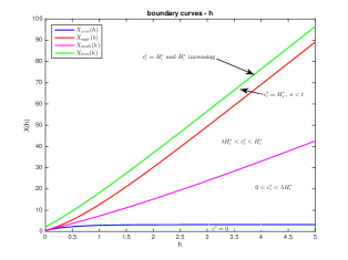
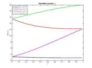
Figure 1: Fix parameters $r=0.05$, $\mu=0.1$, $\sigma=0.25$, $\beta=1$ in both panels. Left panel: graphs of boundary curves in terms of $h$ with $\lambda=0.5$; Right panel: graphs of boundary curves in terms of $\lambda$ with $h=1$.

In particular, the boundary curve $x_{\text{modr}}(1;\lambda)$ in the right panel illustrates that the more the investor cares about the past consumption peak $H_{t}^{*}$, the more conservative the investor will become. This may partially explain the real life situations that the constantly aggressive consumption behavior may not result in a long term happiness. A high consumption plan also creates a high level of psychological competition and hence the aggressive consumption behavior may not be sustainable for the life time. A wise investor who takes into account the past reference will strategically lower the consumption rate from time to time (triggered by a wealth threshold) below the dynamic reference such that the reference process can be maintained at a reasonable level and the overall performance can eventually become a win.

Plugging different pieces of $f$ back into equation (3.23), we can readily get the next result, in which the value function $u$ and optimal feedback controls are all given in terms of the primal variables $x$ and $h$, and the existence of the unique strong solution to SDE (2.1) under optimal controls can be obtained.

Corollary 3.7

For $(x,h)\in\mathcal{C}$ and $0<\lambda<1$, let us define the piecewise function

$$f(x,h)=\left\{\begin{aligned} &\big{(}-x/C_{2}(h)r_{2}\big{)}^{\frac{1}{r_{2}-1}},&&\mbox{if }x\leq x_{\text{zero}}(h),\\ &f_{2}(x,h),&&\mbox{if }x_{\text{zero}}(h)<x<x_{\text{aggr}}(h),\\ &f_{3}(x,h),&&\mbox{if }x_{\text{aggr}}(h)\leq x\leq x_{\text{lavs}}(h),\\ \end{aligned}\right.$$

where $f_{2}(x,h)$ and $f_{3}(x,h)$ are determined by ((ii)) and (3.25). The value function $u(x,h)$ of the control problem in (2.2) is given by

$$u(x,h)$$

$$= \left\{\begin{aligned} &C_{2}(h)f(x,h)^{r_{2}}-\frac{1}{r\beta}e^{\lambda\beta h}+xf(x,h),&&\mbox{if }x\leq x_{\text{zero}}(h),\\ &C_{3}(h)\big{(}f(x,h)\big{)}^{r_{1}}+C_{4}(h)\big{(}f(x,h)\big{)}^{r_{2}}&&\\ &+\frac{f(x,h)}{r\beta}\left(\ln f(x,h)-\lambda\beta h+\frac{\kappa^{2}}{2r}-1+xr\beta\right),&&\mbox{if }x_{\text{zero}}(h)<x<x_{\text{aggr}}(h),\\ &C_{5}(h)\big{(}f(x,h)\big{)}^{r_{1}}+C_{6}(h)\big{(}f(x,h)\big{)}^{r_{2}}-\frac{1}{r}hf(x,h)&&\\ &-\frac{1}{r\beta}e^{(\lambda-1)\beta h}+xf(x,h),&&\mbox{if }x_{\text{aggr}}(h)\leq x\leq x_{\text{lavs}}(h).\\ \end{aligned}\right.$$

To distinguish the feedback functions $c^{\dagger}(y,h)$ and $\pi^{\dagger}(y,h)$ in (3.20) and (3.21) based on dual variables, let us denote $c^{*}(x,h)$ and $\pi^{*}(x,h)$ as the feedback functions of the optimal consumption and portfolio using primal variables $(x,h)$. We have that $c_{t}^{*}=c^{*}(X_{t}^{*},H_{t}^{*})$ and $\pi_{t}^{*}=\pi^{*}(X_{t}^{*},H_{t}^{*})$ where

$$c^{*}(x,h)=\left\{\begin{aligned} &0,&&\mbox{if }x\leq x_{\text{zero}}(h),\\ &-\frac{1}{\beta}\ln f(x,h)+\lambda h,&&\mbox{if }x_{\text{zero}}(h)<x<x_{\text{aggr}}(h),\\ &h,&&\mbox{if }x_{\text{aggr}}(h)\leq x<x_{\text{lavs}}(h),\\ &\frac{1}{(\lambda-1)\beta}\ln\Big{(}\frac{1}{1-\lambda}f\big{(}x,\tilde{h}(x)\big{)}\Big{)},&&\mbox{if }x=x_{\text{lavs}}(h),\end{aligned}\right.$$ (3.30)

where $\tilde{h}(x)$ is given in (3.29), and

$$\pi^{*}(x,h)=\frac{\mu-r}{\sigma^{2}}$$

$$\times\left\{\begin{aligned} &(1-r_{2})x,&&\mbox{if }x\leq x_{\text{zero}}(h),\\ &\frac{2r}{\kappa^{2}}C_{3}(h)f^{r_{1}-1}(x,h)+\frac{2r}{\kappa^{2}}C_{4}(h)f^{r_{2}-1}(x,h)+\frac{1}{r\beta},&&\mbox{if }x_{\text{zero}}(h)<x<x_{\text{aggr}}(h),\\ &\frac{2r}{\kappa^{2}}C_{5}(h)f^{r_{1}-1}(x,h)+\frac{2r}{\kappa^{2}}C_{6}(h)f^{r_{2}-1}(x,h),&&\mbox{if }x_{\text{aggr}}(h)\leq x\leq x_{\text{lavs}}(h).\end{aligned}\right.$$ (3.31)

We have that $0<c_{t}^{*}(X_{t}^{*},H_{t}^{*})<\lambda H_{t}^{*}$ if and only if $x_{\text{zero}}(H_{t}^{*})<X_{t}^{*}<x_{\text{modr}}(H_{t}^{*})$.

Moreover, for any initial value $(X_{0}^{*},H_{0}^{*})=(x,h)\in\mathcal{C}$, the stochastic differential equation

$$dX_{t}^{*}=rX_{t}^{*}dt+\pi^{*}(\mu-r)dt+\pi^{*}\sigma dW_{t}-c^{*}dt$$ (3.32)

has a unique strong solution given the optimal feedback control $(c^{*},\pi^{*})$ as above.

Based on Corollary 3.7, we can readily obtain the next result of the asymptotic behavior of the optimal consumption-wealth ratio $c_{t}^{*}/X_{t}^{*}$ and the investment amount $\pi^{*}_{t}$ when the wealth is sufficiently large. The proof is given in Section 5.1.

Corollary 3.8

For $0<\lambda<1$, as $x\leq x_{\text{lavs}}(h)$, the asymptotic behavior of large wealth $x\to+\infty$ is equivalent to $\lim_{h\to+\infty}x_{\text{lavs}}(h)=+\infty$ thanks to the explicit expression of $x_{\text{lavs}}(h)$ in (3.1). We then have that

$$\lim_{h\to+\infty}\frac{c^{*}(x_{\text{lavs}}(h),h)}{x_{\text{lavs}}(h)}=r,\ \ \ \lim_{h\to+\infty}\pi^{*}(x_{\text{lavs}}(h),h)=\frac{(\mu-r)(1-\lambda)^{r_{1}-1}}{r\beta\sigma^{2}}.$$

As the wealth level gets sufficiently large, the optimal consumption is asymptotically proportional to the wealth level that $c_{t}^{*}\approx rX_{t}^{*}$ and the optimal investment converges to a constant level that $\pi^{*}_{t}\approx(\mu-r)\frac{(1-\lambda)^{r_{1}-1}}{r\beta\sigma^{2}}$. That is, the investor will only allocate a constant amount of wealth into the risky asset and save most of his wealth in the bank account.

3.2 Comparison with Some Related Works

Given the feedback optimal controls in (3.30) and (3.7), we briefly present here some comparison results with Arun Arun and Guasoni et al. GHR on the optimal consumption affected by the past spending maximum. We stress that Arun Arun considers the optimal consumption under a standard time separable power utility that $\sup_{(c,\pi)}\mathbb{E}[\int_{0}^{\infty}e^{-\rho t}\frac{(c_{t})^{p}}{p}dt]$, while the drawdown constraint that $c_{t}\geq\lambda H_{t}^{*}$, $0<\lambda<1$, is only imposed in the set of admissible controls. See also Dybvig Dyb with the ratcheting constraint for $\lambda=1$. A similar optimal dividend control problem with the drawdown constraint is also formulated and studied in Angoshtari et al. BAY. On the other hand, Guasoni et al. GHR studies the optimal consumption under a Cobb-Douglas utility that $\sup_{(c,\pi)}\mathbb{E}[\int_{0}^{\infty}\frac{(c_{t}/H_{t}^{\alpha})^{p}}{p}dt]$, where the utility is defined on the ratio of the consumption rate and the consumption running maximum. By virtue of the power utility on consumption rate, the optimal consumption in Arun Arun and Guasoni et al. GHR automatically satisfy $c_{t}^{*}\geq 0$. On the other hand, we are interested in the exponential utility that measures the difference between the consumption rate and the consumption running maximum process. The non-negativity constraint $c_{t}\geq 0$ needs to be taken care of in solving the HJB equation. As our utility differs from Arun Arun and Guasoni et al. GHR, the feedback optimal consumption is certainly distinct from their results. But we can compare the optimal consumption behavior when the wealth level becomes extremely low and extremely high. These major differences are summarized in Table 1 as below.

	when the wealth is low	when the wealth is high
Arun Arun	the problem is only well defined if the wealth level satisfies the constraint $X_{t}^{*}\geq\frac{a}{r}H_{t}^{*}$; moreover, $c_{t}^{*}=aH_{t}^{*}$ for some $a<1$, i.e., the optimal consumption is proportional to running maximum	$c_{t}^{*}=bX_{t}^{*}$ for some $b>0$, i.e., the optimal consumption is proportional to optimal wealth
Guasoni et al. GHR	when $X^{*}_{t}\leq aH_{t}^{*}$, $c_{t}^{*}=\frac{1}{a}X_{t}^{*}$ for some $a>0$, i.e., the optimal consumption is proportional to optimal wealth	when $X^{*}_{t}\geq bH_{t}^{*}$, $c_{t}^{*}=\frac{1}{b}X_{t}^{*}$ for some $b>0$, i.e., the optimal consumption is proportional to optimal wealth
The present paper	when $X^{*}_{t}\leq x_{\text{zero}}(H_{t}^{*})$, $c_{t}^{*}=0$ even when $X_{t}^{*}>0$	when $X_{t}^{*}=x_{\text{lavs}}(H_{t}^{*})$, $c_{t}^{*}$ is a nonlinear function of $X_{t}^{*}$, as $X^{*}_{t}\rightarrow+\infty$, $c_{t}^{*}\approx rX_{t}^{*}$ that is asymptotically proportional to the optimal wealth

Table 1: Comparison results on optimal consumption when the wealth level is extremely small and extremely large

In addition, in Arun Arun and Guasoni et al. GHR (see also Angoshtari et al. BAY), one can change variables and focus on the new state process $X_{t}/H_{t}$ to reduce the dimension. As a consequence, all thresholds for the wealth variable $x$ separating different regions for the piecewise optimal control in these works are simply linear functions of $h$. In contrary, our utility is defined on the difference $c_{t}-\lambda H_{t}$, and the change of variables is no longer applicable. The HJB equation is genuinely two dimensional that complicates the characterization of all boundary curves separating different regions. We choose to apply the dual transform to $x$ and treat $h$ as a parameter in the whole analysis. The smooth fit principle and inverse transform can help us to identify these boundary curves fully explicitly. We finally can express these thresholds $x_{\text{zero}}(h)$, $x_{\text{aggr}}(h)$ and $x_{\text{lavs}}(h)$ in (3.26), (3.27) and (3.1) as nonlinear functions of $h$ (see the left panel of Figure 1), which are much more complicated than their counterparts in Arun Arun and Guasoni et al. GHR.

4 Numerical Examples and Sensitivity Analysis

We present here some numerical examples of sensitivity analysis on model parameters using the closed-form value function and feedback optimal controls in Corollary 3.7 and discuss some interesting financial implications.

Let us first examine the sensitivity with respect to the weight parameter $0<\lambda<1$ in Figure 2 by plotting some comparison graphs of the value function, the feedback optimal consumption and the feedback optimal portfolio. From the middle panel, we can see again that $x_{\text{zero}}(1;\lambda)$ and $x_{\text{aggr}}(1;\lambda)$ are decreasing in $\lambda$ but $x_{\text{lavs}}(1;\lambda)$ is increasing in $\lambda$. More importantly, for each fixed $x$ such that $x_{\text{zero}}(1;\lambda_{\text{max}})<x<x_{\text{aggr}}(1;\lambda_{\text{min}})$, the feedback optimal consumption $c^{*}(x,1;\lambda)$ is increasing in the parameter $\lambda\in(\lambda_{\text{min}},\lambda_{\text{max}})$, which matches with the intuition that a higher reference weight parameter will induce a higher consumption. However, the middle panel also illustrates that this intuition is only partially correct as it only holds when the consumption does not surpass the historical maximum. When the wealth level gets higher, the investor can freely choose to consume in a lavish way. Then, for $x>x_{\text{lavs}}(1;\lambda_{\text{min}})$, we can see that a smaller $\lambda$ leads to an earlier lavish consumption $c^{*}(x,1)>h=1$ creating a new $h$. But when the wealth continues to increase, the consumption with a larger $\lambda$ will eventually dominate its counterpart with a smaller $\lambda$.

We can also observe from the right panel of Figure 2 that for the fixed $x>0$, $\pi^{*}(x,1;\lambda)$ is decreasing in $\lambda$, which is consistent with the middle panel that the optimal consumption level is lifted up by a larger value of $\lambda$. When the capital is sufficient, the investor may strategically invest less in the market to save more cash to support the higher consumption plan induced by the larger $\lambda$. The left panel of Figure 2 further shows that the value function $u(x,h;\lambda)$ is actually decreasing in $\lambda$. Note that our utility is measured by the difference of the consumption $c_{t}^{*}$ and the reference process $\lambda H_{t}^{*}$. When $\lambda$ increases, both $c^{*}_{t}$ and $\lambda H_{t}^{*}$ increase. We can see from the left panel that $\lambda H^{*}_{t}$ increases faster than the consumption $c^{*}_{t}$ during the life cycle that leads to a drop of $c^{*}_{t}-\lambda H_{t}^{*}$ and the decline in the value function. It is also interesting to observe that when $\lambda$ is large, for $x_{\text{aggr}}(1;\lambda)<x<x_{\text{lavs}}(1;\lambda)$, the optimal portfolio $\pi^{*}(x,1;\lambda)$ may decrease even when the wealth $x$ increases. But when $x$ continues to increase such that $x>x_{\text{lavs}}(1;\lambda)$, we can see that the optimal portfolio $\pi^{*}(x,1;\lambda)$ starts to increase in $x$. That the optimal portfolio might be decreasing in $x$ differs from some existing works and it is a consequence of our specific path-dependent preference. Indeed, when the wealth is sufficient to support the aggressive consumption that $c_{t}^{*}>\lambda H_{t}^{*}$ but the reference process $\lambda H_{t}^{*}$ is not changed, the investor may strategically withdraw the portfolio amount from the financial market to support the consumption plan. This non-standard phenomenon is more likely to happen when the reference parameter $\lambda$ is large such that the resulting consumption $c_{t}^{*}>\lambda H_{t}^{*}$ is very high (see Figure 2), or when the risky asset performance is not good enough (low return as in Figure 3 or high volatility as in Figure 4). However, when $x$ gets abundant such that the investor starts to increase the reference level $\lambda H_{t}^{*}$, the large amount of consumption will quickly eat the capital, and the investor can no longer compromise the portfolio amount to support consumption. It turns to be optimal for the investor to increase the portfolio and accumulate more wealth from the financial market to sustain the extremely high consumption decision. We stress that the non-standard phenomenon that $\pi^{*}(x,1)$ may decrease in $x$ is consequent on some complicated trade-offs of all model parameters. Under some appropriate model parameters, the optimal portfolio $\pi^{*}(x,1)$ is always increasing in $x>0$, which matches with the intuition that we will invest more if we have more.

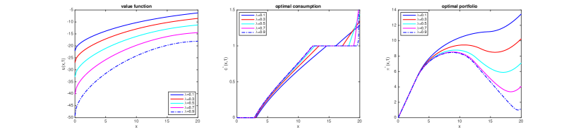
Figure 2: Fix parameters $r=0.05$, $\mu=0.1$, $\sigma=0.25$, $\beta=1$ and the variable $h=1$. With changes of $\lambda=0,1,0.2,0.5,0.7$ and $0.9$, we plot graphs of the value function $u(x,1)$ (left panel), the optimal consumption $c^{*}(x,1)$ (middle panel) and the optimal portfolio $\pi^{*}(x,1)$ (right panel) for $x\in[0,20]$.

We next discuss the impact of the drift parameter $\mu$ based on plots in Figure 3. Firstly, we can see from the left panel that both $x_{\text{zero}}(1;\mu)$ and $x_{\text{aggr}}(1;\mu)$ are decreasing in $\mu$. That is, the higher return the risky asset has, the less wealth that the investor needs to start the positive consumption and initiate the lavish consumption to increase the reference process. Moreover, the feedback optimal consumption is also increasing in $\mu$. These observations are consistent with the real life situation that the bull market will help the investor to accumulate more wealth so that the investor will become more optimistic to develop a more aggressive consumption pattern. Secondly, as one can expect, the right panel of Figure 3 illustrates that the optimal portfolio in the financial market increases as the return increases. In addition, the left panel shows that the primal value function is increasing in $\mu$. It illustrates that when the return $\mu$ increases, the increment in optimal consumption rate $c^{*}_{t}$ dominates the increment in the reference process $\lambda H^{*}_{t}$ so that the value function is lifted up. Thirdly, combining Figure 2 and Figure 3, for the same wealth level $x$, we know that the optimal portfolio $\pi^{*}(x,1;\lambda,\mu)$ is decreasing in $\lambda$ but increasing in $\mu$. As a consequence, for those investors who are more addictive to the past reference level, the market premiums need to be sufficiently high to attract them to invest in the risky asset. This observation may partially explain the observed equity premium puzzle (see Mehra and Prescott Meh and many subsequent works) from the perspective of our proposed path-dependent utility with past spending maximum.

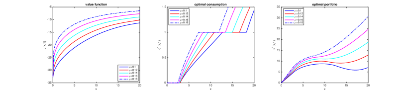
Figure 3: Fix parameters $r=0.05$, $\sigma=0.25$, $\lambda=0.5$, $\beta=1$ and the variable $h=1$. With changes of $\mu=0.10$, $0.12$, $0.14$, $0.16$ and $0.18$, we plot graphs of the value function $u(x,1)$ (left panel), the optimal consumption $c^{*}(x,1)$ (middle panel) and the optimal portfolio $\pi^{*}(x,1)$ (right panel) for $x\in[0,20]$.

At last, we perform sensitivity with respect to the volatility $\sigma$ in Figure $4$. From the middle panel of Figure 4, we observe that the monotonicity of thresholds $x_{\text{zero}}(1;\sigma)$ and the optimal consumption $c^{*}(x,1;\sigma)$ on the parameter $\sigma$ do not hold in general and become much subtle and complicated. Only when the wealth level is sufficiently large, the optimal consumption $c^{*}(x,1;\sigma)$ is decreasing in $\sigma$. It is only clear that the threshold $x_{\text{aggr}}(1;\sigma)$ is increasing in $\sigma$. This observation can be explained that when the wealth level is sufficiently high, the less volatile the risky asset is, the more optimistically the investor will behave in wealth management and consumption plan. In other words, the investor will consume more when $\sigma$ is smaller and lower the threshold to start some large expenditures such that the spending maximum is increased. However, when the wealth level is too low, the investor will become more conservative towards the risky asset account and rely more on interest rate to accumulate enough wealth to initiate a positive consumption. As a consequence, the threshold $x_{\text{zero}}(1;\sigma)$ is not necessarily monotone in $\sigma$. The left and right panels of Figure 4 also show that both the value function and the optimal portfolio are decreasing in the parameter $\sigma$. These graphs are consistent with the real life observations that if the risky asset has a higher volatility, the investor allocates less wealth in the risky asset and the life cycle value function also becomes lower.

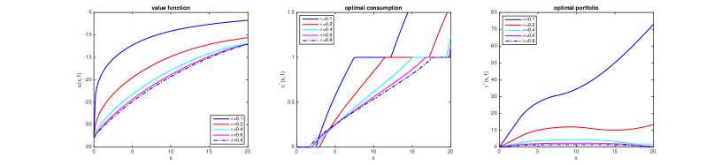
Figure 4: Fix parameters $r=0.05$, $\mu=0.1$, $\beta=1$, $\lambda=0.5$ and the variable $h=1$. With changes of $\sigma=0.1,0.2,0.4,0.6,0.8$, we plot graphs of the value function $u(x,1)$ (left panel), the optimal consumption $c^{*}(x,1)$ (middle panel) and the optimal portfolio $\pi^{*}(x,1)$ (right panel) for $x\in[0,20]$.

5 Proofs of Main Results

5.1 Proofs of some auxiliary results in Section 3

Proof (Proposition 3.2)

We can first obtain the special solution $v(y,h)=-\frac{1}{r\beta}e^{\lambda\beta h}$ for the first equation, then $v(y,h)=-\frac{y}{r\beta}+\frac{y}{r\beta}(\ln y-\lambda\beta h+\frac{\kappa^{2}}{2r})$ for the second equation, and finally $v(y,h)=-\frac{1}{r}hy-\frac{1}{r\beta}e^{(\lambda-1)\beta h}$ for the third equation in (3.12). Therefore, we can summarize the general solution of the ODE (3.12) by

$$v(y,h)=$$

$$\left\{\begin{aligned} &C_{1}(h)y^{r_{1}}+C_{2}(h)y^{r_{2}}-\frac{1}{r\beta}e^{\lambda\beta h},\mbox{if }y\geq e^{\lambda\beta h},\\ &C_{3}(h)y^{r_{1}}+C_{4}(h)y^{r_{2}}-\frac{y}{r\beta}+\frac{y}{r\beta}\left(\ln y-\lambda\beta h+\frac{\kappa^{2}}{2r}\right),\mbox{if }e^{(\lambda-1)\beta h}<y<e^{\lambda\beta h},\\ &C_{5}(h)y^{r_{1}}+C_{6}(h)y^{r_{2}}-\frac{1}{r}hy-\frac{1}{r\beta}e^{(\lambda-1)\beta h},\mbox{if }(1-\lambda)e^{(\lambda-1)\beta h}\leq y\leq e^{(\lambda-1)\beta h},\\ \end{aligned}\right.$$ (5.1)

in which $C_{i}(h)$, $i=1,...,6,$ are functions of $h$ to be determined.

By the explicit form of $v(y,h)$ in (5.1) along the free boundary $y=(1-\lambda)e^{(\lambda-1)\beta h}$, the condition $v_{h}(y,h)=0$ in (3.11) implies that

$$C_{5}^{\prime}(h)(1-\lambda)^{r_{1}}e^{(\lambda-1)\beta hr_{1}}+C_{6}^{\prime}(h)(1-\lambda)^{r_{2}}e^{(\lambda-1)\beta hr_{2}}=0.$$ (5.2)

Similar to the case when $\lambda=0$, the free boundary condition $v_{y}(y,h)\rightarrow 0$ in (3.14) implies that $y\rightarrow+\infty$. Together with free boundary conditions in (3.14) and the formula of $v(y,h)$ in the region $y\geq e^{\lambda\beta h}$, we deduce that $C_{1}(h)\equiv 0$. Moreover, it is easy to see that as $h\rightarrow+\infty$, we get $y\rightarrow 0$ in the third region $(1-\lambda)e^{(\lambda-1)\beta h}\leq y\leq e^{(\lambda-1)\beta h}$ and therefore the boundary conditions in (3.13) also implies the asymptotic condition that $C_{6}(h)\rightarrow 0$ as $h\rightarrow+\infty$.

To determine the remaining parameters, we apply the smooth-fit conditions with respect to the variable $y$ at the two boundary points $y=e^{\lambda\beta h}$ and $y=e^{(\lambda-1)\beta h}$. After simple manipulations, we can deduce the system of equations:

$$\left\{\begin{aligned} &C_{2}(h)e^{\lambda\beta hr_{2}}=C_{3}(h)e^{\lambda\beta hr_{1}}+C_{4}(h)e^{\lambda\beta hr_{2}}+\frac{1}{2r^{2}\beta}e^{\lambda\beta h}\kappa^{2},\\ &C_{2}(h)r_{2}e^{\lambda\beta hr_{2}}=C_{3}(h)r_{1}e^{\lambda\beta hr_{1}}+C_{4}(h)r_{2}e^{\lambda\beta hr_{2}}+\frac{1}{2r^{2}\beta}e^{\lambda\beta h}\kappa^{2},\\ &C_{3}(h)e^{(\lambda-1)\beta hr_{1}}+C_{4}(h)e^{(\lambda-1)\beta hr_{2}}+\frac{1}{2r^{2}\beta}e^{(\lambda-1)\beta h}\kappa^{2}\\ &=C_{5}(h)e^{(\lambda-1)\beta hr_{1}}+C_{6}(h)e^{(\lambda-1)\beta hr_{2}},\\ &C_{3}(h)r_{1}e^{(\lambda-1)\beta hr_{1}}+C_{4}(h)r_{2}e^{(\lambda-1)\beta hr_{2}}+\frac{1}{2r^{2}\beta}e^{(\lambda-1)\beta h}\kappa^{2}\\ &=C_{5}(h)r_{1}e^{(\lambda-1)\beta hr_{1}}+C_{6}(h)r_{2}e^{(\lambda-1)\beta hr_{2}}.\end{aligned}\right.$$

The system of equations can be solved explicitly. To this end, the linear system can be regarded as linear equations in terms of variables $C_{3}(h)$, $C_{2}(h)-C_{4}(h)$, $C_{4}(h)-C_{6}(h)$ and $C_{3}(h)-C_{5}(h)$. We can solve the first two equations and obtain $C_{3}(h)$ explicitly in (3.16) and $C_{2}(h)-C_{4}(h)$. By solving the last two equations, we also get $C_{3}(h)-C_{5}(h)$, which yields $C_{5}(h)$ in (3.18) by substituting the function $C_{3}(h)$.

Plugging the derivative $C_{5}^{\prime}(h)$ back into the boundary condition (5.2), we obtain that

$$C_{6}^{\prime}(h)(1-\lambda)^{r_{2}}e^{(\lambda-1)\beta hr_{2}}= (1-\lambda)^{r_{1}}e^{(\lambda-1)\beta hr_{1}}\frac{(r_{2}-1)\kappa^{2}}{2(r_{1}-r_{2})\beta r^{2}}$$

$$\times\left((\lambda-1)(1-r_{1})e^{(\lambda-1)(1-r_{1})\beta h}-\lambda(1-r_{1})e^{\lambda(1-r_{1})\beta h}\right).$$

By using the asymptotic condition that $C_{6}(h)\rightarrow 0$ when $h\rightarrow+\infty$ and the condition that $\lambda(1-r_{2})-(r_{1}-r_{2})<0$, we can integrate the equation above on both sides, and get $C_{6}(h)$ explicitly in (3.19).

Substituting $C_{6}(h)$ back to

$$(r_{1}-r_{2})\big{(}C_{6}(h)-C_{4}(h)\big{)}e^{(\lambda-1)\beta hr_{2}}=(r_{1}-1)\frac{e^{(\lambda-1)\beta h}}{2r^{2}\beta}\kappa^{2},$$

we can get $C_{4}(h)$ in (3.17). Substituting $C_{4}(h)$ to the equation that

$$(r_{1}-r_{2})\big{(}C_{2}(h)-C_{4}(h)\big{)}e^{\lambda\beta hr_{2}}=(r_{1}-1)\frac{e^{\lambda\beta h}}{2r^{2}\beta}\kappa^{2},$$

we can at last obtain $C_{2}(h)$ in (3.15).

Proof (Lemma 3.5)

We shall analyze each region separately.

(i) In the region $y\geq e^{\lambda\beta h}$, we have $v_{yy}(y,h)=r_{2}(r_{2}-1)C_{2}(h)y^{r_{2}-2}$ as $r_{2}(r_{2}-1)=\frac{2r}{\kappa^{2}}>0$ and $C_{2}(h)>0$ thanks to its expression (3.15). The conclusion holds trivially.

(ii) In the region $(1-\lambda)e^{(\lambda-1)\beta h}\leq y\leq e^{(\lambda-1)\beta h}$, we recall that

$$v_{yy}(y,h)=r_{1}(r_{1}-1)C_{5}(h)y^{r_{1}-2}+r_{2}(r_{2}-1)C_{6}(h)y^{r_{2}-2}.$$

The conclusion easily follows from the fact that $C_{5}(h)>0$, $C_{6}(h)>0$ and the identity that $r_{1}(r_{1}-1)=r_{2}(r_{2}-1)=\frac{2r}{\kappa^{2}}>0$.

(iii) In the region $e^{(\lambda-1)\beta h}<y<e^{\lambda\beta h}$, we proceed by the following two steps:

Step 1: To show $v_{yy}(y,h)>0$, it is equivalent to check that $yv_{yy}(y,h)>0$. Let us first show this at the two endpoints $e^{(\lambda-1)\beta h}$ and $e^{\lambda\beta h}$. So at $y=e^{(\lambda-1)\beta h}$ and $y=e^{\lambda\beta h}$, we need to prove the inequality

$$\frac{2r}{\kappa^{2}}y^{r_{2}-1}\big{(}C_{3}(h)y^{r_{1}-r_{2}}+C_{4}(h)\big{)}+\frac{1}{\beta r}>0.$$ (5.3)

By $C_{3}(h)$ and $C_{4}(h)$ in the explicit form, at the point $e^{\lambda\beta h}$, (5.3) boils down to proving that

$$e^{\lambda\beta h(r_{2}-1)}\frac{1}{(r_{1}-r_{2})\beta}\Bigg{(}e^{\lambda\beta h(1-r_{2})}\frac{r_{2}-1}{r}$$

$$+e^{(\lambda-1)\beta h(1-r_{2})}\frac{1-r_{1}}{r}+\frac{(r_{2}-1)(1-\lambda)^{r_{1}-r_{2}}}{r}$$

$$\times\left(\frac{1-r_{1}}{1-r_{2}}e^{(\lambda-1)(1-r_{2})\beta h}-\frac{\lambda(1-r_{1})}{\lambda(1-r_{2})-(r_{1}-r_{2})}e^{\left(\lambda(1-r_{2})-(r_{1}-r_{2})\right)\beta h}\right)\Bigg{)}+\frac{1}{r\beta}>0.$$

Using the fact that $e^{\lambda\beta h(1-r_{2})}>e^{(\lambda-1)\beta h(1-r_{2})}$, we can see that the above is larger than

$$e^{\lambda\beta h(r_{2}-1)}\frac{1}{(r_{1}-r_{2})\beta}\Big{(}e^{\lambda\beta h(1-r_{2})}\frac{r_{2}-1}{r}+e^{\lambda\beta h(1-r_{2})}\frac{1-r_{1}}{r}\Big{)}+\frac{1}{r\beta}-e^{\lambda\beta h(r_{2}-1)}$$

$$\times\frac{(1-r_{2})(1-\lambda)^{r_{1}-r_{2}}}{(r_{1}-r_{2})\beta r}$$

$$\times\left(\frac{1-r_{1}}{1-r_{2}}e^{(\lambda-1)(1-r_{2})\beta h}-\frac{\lambda(1-r_{1})}{\lambda(1-r_{2})-(r_{1}-r_{2})}e^{\left(\lambda(1-r_{2})-(r_{1}-r_{2})\right)\beta h}\right)$$

$$=-e^{\lambda\beta h(r_{2}-1)}\frac{(1-r_{2})(1-\lambda)^{r_{1}-r_{2}}}{(r_{1}-r_{2})\beta r}$$

$$\quad\times\Bigg{(}\frac{1-r_{1}}{1-r_{2}}e^{(\lambda-1)(1-r_{2})\beta h}-\frac{\lambda(1-r_{1})}{\lambda(1-r_{2})-(r_{1}-r_{2})}e^{\left(\lambda(1-r_{2})-(r_{1}-r_{2})\right)\beta h}\Bigg{)},$$

which is strictly positive. Hence, we have that $yv_{yy}(y,h)>0$ at $y=e^{\lambda\beta h}$.

To show (5.3) at the endpoint $y=e^{(\lambda-1)\beta h}$, it is enough to show that

$$e^{(\lambda-1)\beta h(r_{2}-1)}\frac{1}{(r_{1}-r_{2})\beta}\Bigg{(}e^{(\lambda(1-r_{2})-(r_{1}-r_{2}))\beta h}\frac{r_{2}-1}{r}$$

$$+e^{(\lambda-1)\beta h(1-r_{2})}\frac{1-r_{1}}{r}+\frac{(r_{2}-1)(1-\lambda)^{r_{1}-r_{2}}}{r}$$

$$\times\left(\frac{1-r_{1}}{1-r_{2}}e^{(\lambda-1)(1-r_{2})\beta h}-\frac{\lambda(1-r_{1})}{\lambda(1-r_{2})-(r_{1}-r_{2})}e^{\left(\lambda(1-r_{2})-(r_{1}-r_{2})\right)\beta h}\right)\Bigg{)}+\frac{1}{r\beta}>0.$$

By the fact $e^{(\lambda(1-r_{2})-(r_{1}-r_{2}))\beta h}<e^{(\lambda-1)\beta h(1-r_{2})}$ and similar calculations for $y=e^{\lambda\beta h}$, we can also show that the above term is strictly larger than

$$-e^{(\lambda-1)\beta h(r_{2}-1)}\frac{(1-r_{2})(1-\lambda)^{r_{1}-r_{2}}}{(r_{1}-r_{2})\beta r}$$

$$\times\left(\frac{1-r_{1}}{1-r_{2}}e^{(\lambda-1)(1-r_{2})\beta h}-\frac{\lambda(1-r_{1})}{\lambda(1-r_{2})-(r_{1}-r_{2})}e^{\left(\lambda(1-r_{2})-(r_{1}-r_{2})\right)\beta h}\right)>0,$$

and hence is strictly positive.

Step 2: In this step, we show that the function

$$\gamma(y):=yv_{yy}(y,h)=\frac{2r}{\kappa^{2}}C_{3}(h)y^{r_{1}-1}+\frac{2r}{\kappa^{2}}C_{4}(h)y^{r_{2}-1}+\frac{1}{r\beta}$$

is either monotone or first increasing then decreasing. Combining with Step 1, we can verify the statement of the lemma. Indeed, the extreme point $\breve{y}$ of $\gamma(y)$ should satisfy the first order condition $\gamma^{\prime}(\breve{y})=0$, i.e.

$$C_{3}(h)(r_{1}-1)(y^{*})^{r_{1}-r_{2}}+C_{4}(h)(r_{2}-1)=0.$$

Note that $C_{3}(h)<0$, while $C_{4}(h)$ can be negative or positive. If $C_{4}(h)\leq 0$, there is no solution $\breve{y}$, hence $\gamma(y)$ is monotone. If $C_{4}(h)>0$, there exists a unique real solution to the above equation that

$$\breve{y}=\left(\frac{C_{4}(h)(1-r_{2})}{C_{3}(h)(r_{1}-1)}\right)^{\frac{1}{r_{1}-r_{2}}},$$

which might fall into the interval $[e^{(\lambda-1)\beta h},e^{\lambda\beta h}]$. As we have that $C_{3}(h)<0$ and

$$\gamma^{\prime}(y)=\frac{2r}{\kappa^{2}}y^{r_{2}-2}\big{(}C_{3}(h)(r_{1}-1)(y)^{r_{1}-r_{2}}+C_{4}(h)(r_{2}-1)\big{)},$$

it follows that $\gamma^{\prime}(y)\geq 0$ if and only if $y\leq\breve{y}$. Hence $\gamma(y)$ is increasing in $y$ before reaching $\breve{y}$ and is then decreasing in $y$ after $\breve{y}$.

Proof (Corollary 3.8)

As we consider the asymptotic behavior along the boundary $x_{\text{lavs}}(h)$, we first have

$$\lim_{h\to+\infty}\frac{c^{*}(x_{\text{lavs}}(h),h)}{x_{\text{lavs}}(h)}=\lim_{h\to+\infty}\frac{h}{x_{\text{lavs}}(h)}.$$

Taking into account the explicit form of $x_{\text{lavs}}(h)$ in (3.1), we need to compute the two limits

$$\lim_{h\rightarrow+\infty}\frac{-C_{5}(h)r_{1}(1-\lambda)^{r_{1}-1}e^{(\lambda-1)(r_{1}-1)\beta h}}{h}=\lim_{h\rightarrow+\infty}\frac{\frac{-r_{1}(1-\lambda)^{r_{1}-1}(1-r_{2})\kappa^{2}}{2(r_{1}-r_{2})\beta r^{2}}(1-e^{(1-r_{1})\beta h})}{h}=0$$

and

$$\lim_{h\rightarrow+\infty}\frac{-C_{6}(h)r_{2}(1-\lambda)^{r_{2}-1}e^{(\lambda-1)(r_{2}-1)\beta h}}{h}$$

$$= \lim_{h\rightarrow+\infty}\frac{\frac{-r_{2}(1-\lambda)^{r_{1}-1}(r_{2}-1)\kappa^{2}}{2(r_{1}-r_{2})\beta r^{2}}(\frac{1-r_{1}}{1-r_{2}}-\frac{\lambda(1-r_{1})}{\lambda(1-r_{2})-(r_{1}-r_{2})}e^{(1-r_{1})\beta h})}{h}=0.$$

Therefore, we obtain that

$$\lim_{h\to+\infty}\frac{c^{*}(x_{\text{lavs}}(h),h)}{x_{\text{lavs}}(h)}=r.$$

Similarly, thanks to the explicit form of $\pi^{*}(x,h)$ in (3.7), we need to compute two limits along $x_{\text{lavs}}(h)$ that

$$\lim_{h\rightarrow+\infty}\frac{2r}{\kappa^{2}}C_{5}(h)(1-\lambda)^{r_{1}-1}e^{(\lambda-1)\beta h(r_{1}-1)} =\lim_{h\rightarrow+\infty}\frac{(1-\lambda)^{r_{1}-1}(1-r_{2})}{(r_{1}-r_{2})\beta r}(1-e^{(1-r_{1})\beta h})$$

$$=\frac{(1-\lambda)^{r_{1}-1}(1-r_{2})}{(r_{1}-r_{2})\beta r},$$

and

$$\lim_{h\rightarrow+\infty}\frac{2r}{\kappa^{2}}C_{6}(h)(1-\lambda)^{r_{2}-1}e^{(\lambda-1)(r_{2}-1)\beta h}$$

$$= \lim_{h\rightarrow+\infty}\frac{(1-\lambda)^{r_{1}-1}(r_{2}-1)}{(r_{1}-r_{2})\beta r}\left(\frac{1-r_{1}}{1-r_{2}}-\frac{\lambda(1-r_{1})}{\lambda(1-r_{2})-(r_{1}-r_{2})}e^{(1-r_{1})\beta h}\right)=\frac{(1-\lambda)^{r_{1}-1}(r_{1}-1)}{(r_{1}-r_{2})\beta r}.$$

Therefore, we conclude that

$$\lim_{h\to+\infty}\pi^{*}(x_{\text{lavs}}(h),h) =\frac{\mu-r}{\sigma^{2}}\left(\frac{(1-\lambda)^{r_{1}-1}(1-r_{2})}{(r_{1}-r_{2})\beta r}+\frac{(1-\lambda)^{r_{1}-1}(r_{1}-1)}{(r_{1}-r_{2})\beta r}\right)$$

$$=\frac{(\mu-r)(1-\lambda)^{r_{1}-1}}{r\beta\sigma^{2}}.$$

5.2 Proofs of Theorem 3.3 and Corollary 3.7

Proof (Theorem 3.3)

The proof of the verification theorem boils down to show that the solution of the PDE indeed coincides with the value function. In other words, there exists $(\pi^{*},c^{*})\in\mathcal{A}(x)$ such that

$$u(x,h)=\mathbb{E}\left[\int_{0}^{\infty}e^{-rt}U({c_{t}^{*}-\lambda H_{t}^{*}})dt\right].$$

For any admissible strategy $(\pi,c)\in\mathcal{A}(x)$, similar to the standard proof of Lemma 1 in Arun Arun, we have the following budget constraint:

$$\mathbb{E}\left[\int_{0}^{\infty}c_{t}M_{t}dt\right]\leq x.$$

Regarding $(\lambda,h)$ as fixed parameters, we consider the dual transform of $U$ with respect to $c$ in the constrained domain that

$$V(y,h) :=\sup_{0\leq c\leq h}(U(c-\lambda h)-cy)\;=$$

$$\left\{\begin{aligned} &-\frac{1}{\beta}e^{\lambda\beta h},&&\mbox{if }y\geq e^{\lambda\beta h},\\ &-\frac{1}{\beta}y+y(\frac{1}{\beta}\ln y-\lambda h),&&\mbox{if }e^{(\lambda-1)\beta h}<y<e^{\lambda\beta h},\\ &-\frac{1}{\beta}e^{(\lambda-1)\beta h}-hy,&&\mbox{if }(1-\lambda)e^{(\lambda-1)\beta h}\leq y\leq e^{(\lambda-1)\beta h}.\end{aligned}\right.$$

We remark that when $\lambda=0$, $V(y,h)$ is independent of $h$. Moreover, $V(y,h)$ can be attained by the construction of the feedback function $c^{\dagger}(y,h)$ given in (3.20).

In what follows, we distinguish the two reference processes, namely $H_{t}:=h\lor\sup_{s\leq t}c_{s}$ and $H_{t}^{\dagger}(y):=h\lor\sup_{s\leq t}c^{\dagger}(Y_{s}(y),H_{s}^{\dagger}(y))$ that correspond to the reference process under an arbitrary consumption process $c_{t}$ and under the optimal consumption process $c^{\dagger}$ with an arbitrary $y>0$. Note that the (global) optimal reference process will be defined later by $H_{t}^{*}:=H_{t}^{\dagger}(y^{*})$ with $y^{*}>0$ to be determined. Let us now further introduce

$${\hat{H}_{t}(y)}:=h\lor\Bigg{(}\frac{1}{(\lambda-1)\beta}\ln\left(\frac{1}{1-\lambda}\inf_{s\leq t}Y_{s}(y)\right)\Bigg{)},$$ (5.4)

where $Y_{t}(y)\;=\;ye^{rt}M_{t}$ is the discounted martingale measure density process.

For any admissible $(\pi,c)$ $\in$ $\mathcal{A}(x)$ and all $y>0$, we have that

$$\mathbb{E}\left[\int_{0}^{\infty}e^{-rt}U({c_{t}-\lambda H_{t}})dt\right]= \mathbb{E}\left[\int_{0}^{\infty}e^{-rt}\big{(}U(c_{t}-\lambda H_{t})-Y_{t}(y)c_{t}\big{)}dt\right]$$

$$+y\mathbb{E}\left[\int_{0}^{\infty}c_{t}M_{t}dt\right]$$

$$\leq \mathbb{E}\left[\int_{0}^{\infty}e^{-rt}V\big{(}Y_{t}(y),H_{t}^{\dagger}(y)\big{)}dt\right]+yx$$ (5.5)

$$= \mathbb{E}\left[\int_{0}^{\infty}e^{-rt}V\big{(}Y_{t}(y),{\hat{H}_{t}(y)}\big{)}dt\right]+yx$$

$$= v(y,h)+yx.$$

where the second line follows from Lemma LABEL:lemma:IneqAttained, the third line holds thanks to Lemma LABEL:lemma:ReplaceHat below, and the last line is consequent on Lemma 5.2. In addition, by Lemma LABEL:lemma:IneqAttained, the inequality becomes equality with the choice of $c^{*}_{t}=c^{\dagger}(Y_{t}(y^{*}),H_{t}^{\dagger}(y^{*}))$, in which $y^{*}$ uniquely solves $\mathbb{E}[\int_{0}^{\infty}c^{\dagger}(Y_{t}(y),H_{t}^{\dagger}(y))M_{t}dt]=x$ for the given $x>0$ and $h\geq 0$.

In conclusion, we arrive at

$$\sup_{(\pi,c)\in\mathcal{A}(x)}\mathbb{E}\Big{[}\int_{0}^{\infty}e^{-rt}U({c_{t}-\lambda H_{t}})dt\Big{]}=\inf_{y>0}\big{(}v(y,h)+yx\big{)}=u(x,h),$$

which completes the proof of the verification theorem. ∎

We then proceed to prove some auxiliary results that have been used to support the previous proof of the main theorem. We shall use the following asymptotic results of the coefficients defined in Proposition 3.2.

Remark 5.1

Based on the explicit formulas in (3.15)-(3.17), we note that as $h\to+\infty$, we have the asymptotics

$$C_{2}(h)=O\left(e^{(\lambda-1)(1-r_{2})\beta h}\right)+O\left(e^{(\lambda(1-r_{2})-(r_{1}-r_{2}))\beta h}\right)+O\left(e^{\lambda(1-r_{2})\beta h}\right),$$

$$C_{3}(h)=O\left(e^{\lambda\beta h(1-r_{1})}\right),$$

$$C_{4}(h)=O\left(e^{(\lambda-1)(1-r_{2})\beta h}\right)+O\left(e^{(\lambda(1-r_{2})-(r_{1}-r_{2}))\beta h}\right),$$

$$C_{5}(h)=O\left(e^{\lambda\beta h(1-r_{1})}\right)+O\left(e^{(\lambda-1)(1-r_{1})\beta h}\right),$$

$$C_{6}(h)=O\left(e^{(\lambda-1)(1-r_{2})\beta h}\right)+O\left(e^{(\lambda(1-r_{2})-(r_{1}-r_{2}))\beta h}\right).$$

Lemma 5.2

$$v(y,h)=\mathbb{E}\left[\int_{0}^{\infty}e^{-rt}V\big{(}Y_{t}(y),\hat{H}_{t}(y)\big{)}dt\right].$$