Max-Min Lyapunov Functions for Switched Systems
and Related Differential Inclusions
Abstract
Starting from a finite family of continuously differentiable positive definite functions, we study conditions under which a function obtained by max-min combinations is a Lyapunov function, establishing stability for two kinds of nonlinear dynamical systems: a) Differential inclusions where the set-valued right-hand-side comprises the convex hull of a finite number of vector fields, and b) Autonomous switched systems with a state-dependent switching signal. We investigate generalized notions of directional derivatives for these max-min functions, and use them in deriving stability conditions with various degrees of conservatism, where more conservative conditions are numerically more tractable. The proposed constructions also provide nonconvex Lyapunov functions, which are shown to be useful for systems with state-dependent switching that do not admit a convex Lyapunov function. Several examples are included to illustrate the results.
1 Introduction
Lyapunov functions play an instrumental role in the stability analysis of dynamical systems; The textbook [25] and the research monographs [4] and [29] provide an overview of the developments in this field. When considering dynamical systems resulting from switching among a finite number of dynamical subsystems described by ordinary differential equations (ODEs) of the form , , locally Lipschitz continuous, , different constructions of Lyapunov functions are proposed in the literature to analyze stability of the common equilibrium point: the origin. Overviews of such methods and related references can be found in [26], [38], and [28].
When the evolution of state trajectories results from arbitrary switching among the individual subsystems, the stability analysis problem is equivalently addressed by considering the differential inclusion (DI), described by
| (1) |
where denotes the convex hull of the set . For the linear differential inclusion (LDI) case (that is for some ), it is shown in [13], [31] that asymptotic stability is equivalent to the existence of a common Lyapunov function that is convex, homogeneous of degree 2, and . By addressing a similar question, the paper [30] establishes the existence of a common homogeneous polynomial Lyapunov function for asymptotically stable LDIs. Various parameterizations can approximate such homogeneous convex functions, such as maximum of quadratic functions and its convex conjugates [17], [19], which are shown to be universal in [20]. Constructions involving functions with convex polyhedral level sets are proposed in [31] and in [7]. These functions are mostly locally Lipschitz but not continuously differentiable, therefore the notion of set-valued derivatives, studied in [10, Chapter 2], [3], is important. Results analyzing nonsmooth Lyapunov functions using such notions of derivatives appear in [9], [39], [11, Chapter 4]. For general differential inclusions, converse Lyapunov theorems are proved in [40]. Other techniques for constructing common Lyapunov functions come from imposing strong structural assumptions, such as commuting vector fields [32], triangular structure or solvability/nil-potency of the Lie-algebra generated by [27]. Without any structural conditions, the Lyapunov functions for system (1) are, in general, not finitely constructible.
On the other hand, for discrete-time systems with arbitrary switching, some constructions involving combinatorial methods have recently appeared. Path-complete Lyapunov functions are proposed in [1] to approximate the joint spectral radius, and it is shown in [2] that this class of functions can be written more explicitly in the form of maximum and minimum over a set of smooth functions. Our conference paper [15] uses the construction based on max-min of smooth functions to study stability of the continuous-time system (1) using Clarke’s derivative, and this article provides new results in this direction.
In contrast to studying stability uniformly over all possible switching signals as in (1), it is also of interest to study dynamical systems driven by a given switching function , resulting in
| (2) |
so that the solution set for system (2) is a strict subset of the solution set of system (1). As already mentioned, existence of a convex Lyapunov function is necessary for asymptotic stability of LDIs. However, it is possible that system (2) is asymptotically stable with fixed, but does not admit a convex Lyapunov function [8]. It is possible to provide sufficient conditions for a minimum of quadratics (clearly non-convex) to be a Lyapunov function in this context, see [21] and [41]. In general, constructions involving piecewise quadratic functions have been found quite useful [23], and LMI-based formulations have been proposed to compute such functions [14], [36]. Beyond piecewise quadratics, sum-of-squares techniques have been used for polynomial Lyapunov functions [35].
In this article, the problem of interest is to construct a Lyapunov function for systems (1) and (2) which guarantees asymptotic stability of the origin . We consider the Lyapunov functions obtained by taking the maximum, minimum, or their combination over a finite family of continuously differentiable positive definite functions, see Definition 3 for details. Such max-min type of Lyapunov functions were recently proposed in the context of discrete-time switching systems [1], [2]. For the continuous-time case treated in this paper, studying this class of functions naturally requires certain additional tools from nonsmooth and set-valued analysis, and one such fundamental tool is the generalized directional derivative. In our conference paper [15], we provide stability results based on Clarke’s notion of generalized directional derivative for max-min functions. The construction of non-smooth Lyapunov functions for system (2) using the Clarke’s generalized gradient concept is also presented in [5]. However, this notion turns out to be rather conservative as is seen in several examples (including the one given in Section 2). To overcome this conservatism due to Clarke’s generalized derivative, we work with the set-valued Lie derivative, which is formally introduced in Definition 2. Focusing on this latter notion of generalized directional derivative for the class of max-min Lyapunov functions, the major contributions of this paper are listed as follows:
-
•
Describe max-min functions and study generalized notions of set-valued derivatives for such functions.
- •
- •
The notion of set-valued Lie derivative was introduced in [3] for locally Lipschitz regular functions. In the context of stability analysis of a differential inclusion, the set-valued Lie derivative was used in [24] to identify and remove infeasible directions from the differential inclusion. For the max-min candidate Lyapunov functions studied in this paper, which are not regular in general, we compute set-valued Lie derivatives and use them to derive stability conditions for systems (1) and (2). The resulting conditions turn out to be less conservative than the ones obtained by using Clarke’s derivative in [15], which are here recovered as a corollary. When restricting the attention to the linear case , and max-min functions obtained from quadratic forms, the Lie-derivative conditions require solving nonlinear matrix inequalities.
It should be noted that, since we allow for the minimum operation in the construction, certain elements in our proposed class of Lyapunov functions are nonconvex. In our approach, when we construct a homogeneous of degree 2 nonconvex Lyapunov function for the LDI problem, a convexification of such functions also provides a Lyapunov function [19, Proposition 2.2]. In fact, the sublevel sets of max-min functions approximate the convex sublevel sets of a homogeneous of degree 2 convex Lyapunov function (which is known to exist) with nonconvex sets obtained via intersections and unions of ellipsoids.
When addressing system (2), our approach provides a more general class of nonconvex and nondifferentiable Lyapunov functions obtained via max-min operations. To describe the solutions of switched systems, we adopt Filippov regularizations [16], and establish stability conditions for the resulting system. Considering such regularized differential inclusions for the switched systems also allows considering sliding motions along the switching surfaces. In this setting, our adopted notion of set-valued Lie derivative turns out to be crucial and has an interesting geometrical interpretation in terms of the tangent subspace to the switching surface.
The paper is organized as follows: In Section 2 we provide an example of a two-dimensional switched system that does not admit a convex Lyapunov function, but a max-min Lyapunov function can be found. In Section 3 we introduce generalized notions of derivatives for Lipschitz continuous functions, while in Section 4 the class of max-min functions is presented and we show our main stability results in the setting of differential inclusions. In Section 5 we apply our results to switched systems, written as a differential inclusion using Filippov regularizations, and we study asymptotic stability along with an instructive example. In Section 6, we analyze deeply the case of linear switched systems and propose an algorithmic procedure to construct max-min Lyapunov functions, followed by some concluding remarks in Section 7.
2 A Motivating Example
We consider a switched system for which there does not exist any convex Lyapunov function. However, this system is asymptotically stable and our results will allow constructing a Lyapunov function defined as
| (3) |
for some positive definite matrices , . This example was introduced in [15] where we did not include the proof of Proposition 1, given below.
Example 1.
Consider a linear switched system as in (2), with three subsystems and a state-dependent switching rule , namely
| (4) |
where To define the switching signal , introduce matrices
and the switching signal
| (5) |
where the subspaces , are defined as , namely
We note that in (5), we have and that the only point of intersection among the three sets is the origin.
Proposition 1.
There does not exist a convex Lyapunov function for system (4).
Proof.
Given a set and a time , let be the set of reachable points of solutions of system (4) after time , starting in , that is,
Following [8, Lemma 2.1], if we show that there exists a compact set and a such that (where is the convex hull of ) then the system does not admit a convex Lyapunov function.
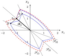
Toward this end, we choose , and the compact set , i.e. the line segment connecting and . We compute
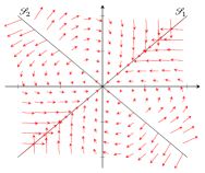
which allows us to write analytically the solution of the system starting from any given initial condition. We let be the smallest time such that , and be the smallest time such that . We finally choose as the smallest time such that . It turns out that . Thus, the half turn, starting with and reaching , decreases the norm of the state by a factor of . Due to the central symmetry of the dynamics (that is, if is a solution, then is also a solution) the solution will reach the set at the point at time . Hence, the set is (strictly) contained in the set . To show that , it thus remains to check that
| (6) |
Property (6) is graphically illustrated in Figure 1 and is proven by the fact that points and satisfy and , and thus , and . Having already shown that , property (6) indeed holds. ∎
3 Generalized Gradients and Directional Derivatives
The function in (3) is nonsmooth and requires generalized notions of gradient and directional derivatives, recalled here from [10, Chapter 2], [9].
Let be an upper semicontinuous111 A set-valued map is said to be upper semicontinuous at if, for every there exists a such that if then . It is said to be upper semicontinuous if it is upper semicontinuous at every . For comparisons with a related notion of outer semicontinuity, see [18, Lemma 5.15]. map with nonempty, compact, convex values, and consider the differential inclusion (resembling dynamics (1) and (2)),
| (7) |
We recall that a solution of on an interval is a function such that is absolutely continuous, , and for almost all . In the case the solution is said to be complete. The origin of (7) is asymptotically stable (AS) if it is Lyapunov stable (for each such that all solutions satisfy , ) and attractive (there exists such that solutions satisfying .) If attractivity is global (it holds for every ), then we say that the origin is globally asymptotically stable (GAS). We are only concerned with stability of the origin in this article, and use the statement that a system is (G-)AS to refer to the stability of the origin for the corresponding system. Given an open and connected set such that , we say that a locally Lipschitz function is a Lyapunov function for (7) if there exist class functions222A function is positive definite () if it is continuous, , and if . A function is class () if it is continuous, , and strictly increasing. It is said to be class if it is class and unbounded. , and a positive definite such that
and there exists a such that given any solution of (7) with , we have
The existence of a Lyapunov function implies the asymptotic stability of system (7). If moreover , and can be arbitrarily large, the existence of such a implies global asymptotic stability of (7), see [25, Chapter 4]. Given an open set and a locally Lipschitz function we first consider the Clarke’s generalized gradient [10, Chapter 2], which, due to the equivalence in [10, Theorem 2.5.1, page 63] can be defined as
| (8) |
where is the set of measure zero where is not defined. [10, Theorem 2.5.1, page 63] proves the existence of at least one sequence as considered in (8), namely , for all . Moreover, the following property of locally Lipschitz functions will be used in what follows.
Definition 1.
Given an open set , a locally Lipschitz function is regular at if, for every , the directional derivative exists and the equality
| (9) |
holds. is called regular if it is regular at each .
Definition 1 is in fact a characterization of regularity for locally Lipschitz functions, which follows from [10, Proposition 2.1.2]. For an alternative definition we refer to [10, Definition 2.3.4]. The right-hand side of (9) is also called the Clarke’s generalized directional derivative of at along (denoted by and defined in [10, Section 2.1]). The results of this paper could be equivalently stated by referring to Clarke’s generalized directional derivatives instead of the Clarke’s generalized gradient in (8), but we believe that the gradient is a more familiar concept in the control community.
We now introduce two different notions of the generalized directional derivative with respect to differential inclusions (7). We will show that the first one, the more “natural” one, leads to more conservative stability results than the second one. In particular the second one is needed for proving GAS of the motivating example introduced in Section 2.
Definition 2 ([3, 12]).
Consider the differential inclusion (7); given an open set and a locally Lipschitz function . Given , the Clarke’s generalized derivative of with respect to is defined as
| (10) |
Additionally, we define the set-valued Lie derivative of with respect to as
| (11) |
In the case where is continuously differentiable at , one has and . Moreover, it is clear that
| (12) |
In fact, given , there exists such that , for all and thus in particular . Intuitively, it means that when defining we do not consider every possible scalar product between vectors of and , rather we only consider directions that are “meaningful” in the sense of possible flowing directions of solutions. Recalling that the Euclidean scalar product is bilinear in its arguments and, for each , is continuous, it can be shown that, for each fixed , and are compact intervals, possibly empty. Concluding this section, we illustrate the differences between the different notions of set-valued derivatives in the following example.
Example 2.
Consider the function defined as , which is differentiable everywhere except at and Lipschitz continuous. From (8), Clarke’s generalized gradient at 0 is . Now let us suppose that a set-valued map is given such that . Using (10), we compute
On the other hand, using (11) and noting that for each if and only if , we get
It is easily verified that is a subset of .
4 Stability Using Max-Min Functions
In this section, we use the generalized derivatives to study a particular class of locally Lipschitz Lyapunov functions establishing sufficient stability conditions for system (1).
4.1 Max-Min Functions
The following definition was introduced by [2] in the context of path-complete Lyapunov functions for discrete time switching systems.
Definition 3.
Consider an open and connected set . Given base functions , a max-min function is either defined as
| (13a) | ||||
| for some and nonempty sets , or | ||||
| (13b) | ||||
for some and nonempty sets .
The following proposition states the equivalence between (13a) and (13b), which is obtained by applying the distrubutive property of the operators. For a formal proof we refer to [33] and references therein. In the sequel, all our derivations apply to both equivalent expressions (13a) and (13b) but for definiteness, we use the notation adopted in (13a).
Proposition 2.
We denote by the set of all the possible max-min functions obtained from base functions . Given , it is noted that at each point where a strict ordering holds between the values of the base functions, that is, , the function value coincides with , for some . At points where two or more base functions are equal, the function may switch between different base functions. For every , we may define the set where the function is active, more precisely
| (14) |
which are closed by continuity of . We can associate a mapping with every . This map is useful to characterize the generalized derivatives introduced in Definition 2.
Definition 4 (Essentially-active index map).
Given a function , the corresponding essentially-active index map is defined as
| (15) |
where and represent the closure and the interior of a set , respectively. Indexes are called essentially-active indexes of at .
It will be shown in Lemma 1 that is nonempty, for every . Here, instead, we highlight that
| (16) |
The set appearing in the right-hand side of inclusion (16) is called active index set in the context of piecewise functions, for example in [34] and [37, Chapter 4]. To obtain the inclusion (16), consider any , then from Definition 4 and being open, there is a sequence such that , . By continuity of and , we have .
We emphasize that, in general, the inclusion in (16) is strict and equality does not necessarily hold.
Moreover, given , the map contains all the necessary information to locally describe the function , as formalized in the following result.
Lemma 1.
Consider . For each the set is non empty and there exists a neighborhood of such that
| (17) |
4.2 Gradients and Stability Conditions
The following statement draws connections between Clarke’s generalized gradient and the set-valued Lie derivative in (11) for a generic , using the mapping .
Proposition 3.
Given and , the following equality holds
| (18) |
In particular, given , the Lie derivative in (11) reads
| (19) |
Proof.
We now propose a sufficient condition for asymptotic stability of system (7) in terms of given in (19), while adopting the convention that .
Theorem 1.
Given system (7), an open and connected set such that , and positive-definite functions , consider a max-min function with given in (19). If there exists a function such that, for every ,
| (20) |
then is a Lyapunov function and system (7) is AS. If and in addition, each , , is radially unbounded, then the origin of (7) is GAS.
A fundamental result for proving Theorem 1 appears in Lemma 2 given below. The proof of Lemma 2 with some related discussions is deferred to Section 4.4.
Lemma 2.
Consider a function and a solution of the differential inclusion (7). For ,
| (21a) | |||
| (21b) | |||
Remark 1 (Comparison with other approaches).
In Lemma 2, we relate the Dini derivative of along the solutions of system (7) with the Lie derivative . In [11, Chapter 4.2], we also see a relationship between the Dini derivative and the directional derivative along vector fields in the context of weak stability. In particular, it is shown that for every , , for almost every . On the other hand, for strong stability, it would be natural to work with the relation, , for every . However, such a relation is conservative for our purposes, as it can be seen in Example 1 (see Remark 9), where the supremum on the right-hand side of the foregoing inclusion is strictly positive along certain directions in the set for some . The use of Lie derivative in Lemma 2 thus provides tighter bounds on the Dini derivative by selecting meaningful directions from the set for each .
Remark 2.
Stability results involving the set-valued Lie derivative (11) and condition (20) are proved in [3, Proposition 1] for locally Lipschitz and regular (recall Definition 1) Lyapunov functions. Set-valued Lie derivatives are also used in [24] to identify and remove infeasible directions from a differential inclusion when limiting the attention to regular locally Lipschitz functions. Showing that this condition is sufficient when considering locally Lipschitz functions obtained via a max-min composition nontrivially generalizes such results. In fact, a function is in general not regular: recalling (18), the definition in (9) requires, for a regular function , that
| (22) |
for all and for all . However considering for example , we have that the left-hand side of (22) is equal to , and thus in general equality (9) doesn’t hold. In this sense Lemma 2 is a generalization of [3, Proposition 1] to a class of nonregular functions.
Recalling inclusion (12), we can state the following result specifically for (1), using the notion of Clarke’s generalized derivative, which is generally more conservative than Theorem 1. This result is also reported in our preliminary conference paper [15, Theorem 1].
Corollary 1.
Consider the DI (1). Given an open and connected set such that and positive-definite functions , consider a max-min function . Suppose that there exists a function , such that for all ,
| (23) |
for all . Then the origin of (1) is AS and is a Lyapunov function for system (1). If , and in addition, each , , is radially unbounded, then the origin of (1) is GAS.
Proof.
4.3 Proof of Lemma 1
Proof.
Case 1: Consider first the case where for an and for all . By continuity of there exists a neighborhood of where the non-equality relations are preserved and thus , which implies and , in addition to (17) with .
Case 2: Let us now consider the general case and if , for some . By continuity of there exists a neighborhood of such that the non-equality relations , are conserved, for any . Recalling (16), ; when , we are done, by proceeding exactly as in Case 1. Otherwise, when consider without loss of generality, that . By Definition 4, implies therefore there exists an open neighborhood of such that
| (24) |
Consider now, if any, each point such that and , for all , it again follows from continuity that for every , and every in some neighborhood of . Moreover we have, by our choice of , if for every , which implies , . As a consequence , and by equation (24) we have . In other words, we have shown that
| (25) |
Now, if , (17) holds with and . Otherwise we can iterate this argument supposing and so on. At each iteration , generalizing (24) and (25), we construct an open neighborhood of such that and
| (26) |
Either and the proof is complete with or we need to iterate again. Note that when , the existence of as in (26), implies , for all , thus proving and hence . This completes the proof of (17) and the fact that is non-empty. ∎
4.4 Proof of Lemma 2
Lemma 2 is the key result used in the proof of Theorem 1, establishing properties of the directional derivative of along the solutions of (7). In its proof we will use the following result.
Claim 1.
Given functions continuous at , we have that
Proof of Claim 1.
Define for all ; is continuous at since it is the pointwise minimum of continuous functions. We have
thus concluding the proof. ∎
Proof of Lemma 2.
Recalling that is an absolutely continuous solution of the differential inclusion (7) and that is a locally Lipschitz function, the function is absolutely continuous, and hence exists almost everywhere in , proving (21a). Moreover, there exists a set of measure zero such that, for every , both and exist, and .
To prove (21b), from Proposition 2, we use representation (13b) of , dropping the superscript “” for notational simplicity, that is
where and are non-empty subsets of . By Lemma 1, for each , and for each in a neighborhood of , can be expressed as
namely only the active indexes in play a role (possibly ruling out the sets for which ). Let us introduce the notation
| (27) |
To proceed in a constructive manner, consider the set containing all the functions obtained by max (and only max) combination over . The cardinality of is finite and equal to and we can denote its elements by , for . Reasoning as before, for each define as the subset of where is not differentiable. Since are locally Lipschitz, then each has measure zero. Fix any . From the fact that in (27) is locally Lipschitz for each , we obtain
| (28) |
where the limit exists because . The functions in (27) are regular (Definition 1). We can follow the idea of [3, Lemma 1]: by letting go to zero from the right, recalling inclusion (16), we get
| (29) |
Similarly, by letting go to zero from the left in (28), we get
| (30) |
Since exists, we have (29)=(30), and thus for each we can write, for all ,
| (31) |
Now consider the function , for in some neighborhood of . For all , we use the fact that for all , to obtain
Then, applying Claim 1 and (31) we have
| (32) |
Using again Claim 1, we can also write
| (33) |
Summarizing, from (32) and (33), it follows that . Therefore, from (31) we get, for each , that implies . Finally, recalling that , we have
5 Switched systems
We now focus our attention on system (2). In contrast to (1), where the vector fields may switch to any value at any point in the state space, the switching in (2) occurs according to the pre-specified function , which determines the active vector field as a function of the state. As a consequence, solutions of (2) are also solutions of (1) and Theorem 1 also implies GAS of (2). However we search here for less conservative stability conditions. Let be in (2). The class of switching functions that we consider for system (2) is introduced in the following assumption.
Assumption 1.
There exist finitely many analytic functions , defining open sets by
such that is constant and equal to on each ,
Note that, in Assumption 1 the value of remains unspecified on , i.e. the boundaries of , . Since , and the set of zeros of an analytic function has zero Lebesgue measure, this ambiguity will not affect the solution set of (2), as explained in the sequel.
Given and satisfying Assumption 1, we define , as
| (34) |
Because the vector field in (34) is in general discontinuous, we define an appropriate notion of solution of (34), arising from the Filippov regularization.
Definition 5 ([16]).
For the vector field in (34), the computation of is simplified as observed in [12, Page 51] and is summarized below:
Proposition 4.
We underline that under Assumption 1 the Filippov regularization is an upper semi-continuous map with being nonempty, compact, and convex for each . Thus, we can study stability of switched systems in (34) using the results developed in Section 4. Defining as in (19) with replaced by , Theorem 1 leads to the following statement in the context of switched systems.
Theorem 2.
Theorem 2 simultaneously accounts for points where (associated to ), and/or points where (associated to ) are multivalued. Interesting things happen when these points coincide, namely when mimics the patchy shape of .
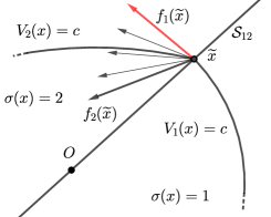
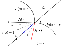
Remark 3.
Consider the simplest non-trivial case, taking an such that and , for some . We may give a geometric interpretation of (39). Parameterizing an with in expression (19), we have that , if and only if there exists such that (we omit the argument of the gradients to simplify the notation),
which holds only if
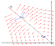
It follows that only if the vector fields and are such that the inner product of their respective components, normal to the hypersurface is negative, namely they do not point both on the same side of . Figure 2 provides an illustration of this fact in the planar case.
In Example 3, an illustration of this idea is provided.
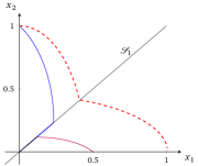
Example 3.
We consider a system of the form (2) and analyze its stability using Theorem 2. Given , and , consider the switched system
| (40) |
where , and function is defined as
System (40) can be written as (34), and satisfies Assumptions 1 with .
Consider now ,
we prove that is a Lyapunov function in the sense of Theorem 2.
Noting that , we can say that the points where is not differentiable coincide with the points where is not continuous. To show inequality (39), we proceed in three steps:
Step 1: Each subsystem is GAS.
Analyzing each subsystem where is differentiable, it can be shown that
The next step is to check the inequality (39) where is not differentiable, that is on the lines and , so that is the set where .
Step 2: Line with converging sliding motion. We compute the set-valued derivative for a point . Proceeding as in Remark 3, based on (19), it is seen that
| (41) |
holds with , for every . Consequently, for each , we have
. By construction, the same singleton would be obtained if we replaced by .
Substituting the values of and , , it thus follows that , .
In Figure 3(a), we have plotted two converging “sliding” solutions.
Step 3: Line with diverging sliding motion.
Choosing , and following the same reasoning as in Step 2, it is seen that the set is nonempty because (41) holds with , for every . As a result, .
Analyzing the linear term, we have
; for the nonlinear term, for each , we have
For small enough, we see that where . Thus, for sufficiently large values of , there exists a such that
| (42) |
if and .
Combining the three steps we proved (39) (with ) for a small open neighborhood of the origin, and Theorem 2 establishes local asymptotic stability of the origin by using the minimum of two quadratics as a Lyapunov function.
Condition (39) fails to be true on the line , away from the origin regardless of the selection of . Hence, there exist Filippov solutions, starting in with large enough initial condition that stay in and diverge; see Figures 3(b) and 3(c) for an illustration.
We want to underline that, since for all , recalling (10), it holds that , . This observation again shows the utility of using Lie derivative compared to Clarke’s derivative in (10), which does not allow establishing asymptotic stability of the origin.
6 Linear Switched Systems and Quadratic Basis
We are now interested in applying Theorem 2 to switched systems (34) with linear vector fields and a partition given by symmetric cones. More precisely, given , we consider the differential inclusion
| (43) |
The set valued map arises from a switching function satisfying Assumption 1, where the sets are defined by
| (44) |
with properly chosen symmetric matrices and not negative semidefinite for each . The sets in (44) are symmetric open cones (if then for all ). The map in (37), can be rewritten in this context as follows:
Indeed not negative semidefinite implies .
Remark 4.
Another possible kind of partition of the state space arises by considering polyhedral cones (with a common vertex at the origin), that is sets (satisfying Assumption 1) defined by linear inequalities , where , for all and denotes the component-wise relation. The techniques employed in what follows could be adapted also to this case.
We restrict our attention to Lyapunov functions homogeneous of degree 2, considering max-min functions obtained from quadratic forms. This choice is motivated by the fact that, as proved in [20], max of quadratics Lyapunov functions are universal (existence is sufficient and necessary) for GAS of linear differential inclusions (LDI). For linear state-dependent switched systems (43), as we noted, non-convex (but still homogeneous) Lyapunov functions are required, and thus the min-operator was added to have this flexibility. The study of universality for max-min of quadratics for (43) is open for further research. The construction of “piecewise” quadratic Lyapunov functions, in similar settings, is studied also in [23], [19], and references therein.
Definition 6.
Given distinct, symmetric and positive definite matrices , a max-min of quadratics is denoted by , and is defined as
| (45) |
where and for each , the set is nonempty.
Remark 5 (Homogeneity).
6.1 Stability Conditions with Set-Valued Lie Derivative
We first specialize the conditions of Theorem 2 for system (43) with of the form (45). To this end, points where is a singleton are easily characterized because they satisfy . Instead, consider any , such that with , namely any point where the locally Lipschitz function is not continuously differentiable. Define now the probability simplex of dimension as
Denoting , and proceeding as in Remark 3, by (19) we have that if and only if there exist such that
| (46) |
for each . Based on (46), define the set as
| (47) |
where . Then, recalling (19), we have
| (48) |
The equivalence (48) is used to prove the next corollary of Theorem 2.
Corollary 2.
Consider system (43) and a max-min of quadratics , where are symmetric, positive-definite, and pairwise distinct matrices. Suppose that there exists such that
-
(i)
For each with and being singletons, it holds that
(49) -
(ii)
For each satisfying , with , and with , there exists such that
(50) for all .
Then the origin of (43) is GAS.
Proof.
It follows from Theorem 2 that the origin of (43) is GAS if (39) holds for all . We will proceed by analyzing four cases, depending on whether the sets and are singletons or not.
First, consider such that and are singletons. In this case,
where the inequality is due to condition (i).
Secondly, for a point with , with , and with , it follows from (48) and condition (ii) that .
Next, consider the case where is a singleton and with , that is a point where is continuously differentiable and the set in (43) is multivalued. We thus have , and from linearity we have
| (51) |
where . Since , by (37) ; from item (i) we have
for some sequence with , .
By continuity we thus have , and from (51) we have
.
Finally, we consider the case with and , namely a point where the function is not continuously differentiable and the set is a singleton, since .
If we are done. Otherwise, in view of (47), implies
| (52) |
Considering, without loss of generality, the index , by Definition 4 and recalling that is open, we can consider a sequence such that , for all . By condition (i) we have
By continuity ; recalling (52), it implies that
.
Having analyzed all the cases, we conclude that (39) holds for all and the assertion follows from Theorem 2.
∎
6.2 Checking Item (i) of Corollary 2
In this section, we exploit the properties of system (43) and the family of candidate max-min Lyapunov functions in (45) to computationally check condition (i) of Corollary 2. We do so by following two steps: first, fixing , , nonempty subsets , and hence the corresponding max-min combination in (45), we construct an auxiliary function , which characterizes the regions where is single-valued. Notably, this function is independent of . Secondly, we use to compute matrices satisfying item (i) of Corollary 2 by only checking the feasibility of a finite set of matrix inequalities. The details of implementing these two steps now follow:
Step 0.
Consider the symmetric group of order denoted by , which is the group of all possible permutations of the first positive integers. Given any pairwise distinct quadratic functions associated to some , for any , define the open set
| (53) |
which is a cone (possibly empty) where a strict ordering among the quadratic functions holds. For a given max-min combination in (45), namely given and nonempty sets , , in each the function defined in (15) is constant and single valued; let us denote it by .
In Algorithm 1, we present how to numerically construct , independently of matrices .
Remark 6.
We emphasize that function is independent of , but only depends on the max-min policy defined by sets . As an example, considering and , the max-min combination (45) coincides with the maximum of the quadratic functions. In this case, will be defined as because of (53). Also, to relate with , it is seen that for any base quadratics defined by with a specific max-min combination determined by , the mapping in (15) corresponds to
Step 1 (Conditions on ).
Consider system (43), and take , and nonempty sets. Find , , , , , and , such that
| (54) |
In Proposition 5 below, we prove that the feasibility of Step 1 yields matrices such that condition (i) of Corollary 2 holds, while in Algorithm 2 we formalize this step of computationally checking condition (54).
Proposition 5.
Proof.
Remark 7 (Polyhedral cones).
Consider again the alternative state-space partition discussed in Remark 4. More precisely, consider polyhedral cones defined by , where, for each , for some . Equivalently, the sets can be represented by , where are the rays of the cone . Let us call by the matrix whose columns are the vectors . As presented in [22, Lemma 1] we have that, given any symmetric matrix , if there exists a symmetric and entry-wise positive matrix such that then . Using this result, the procedure presented in Step 1 and Proposition 5 can be adapted to the polyhedral cones case by requiring that for any , any and any , there exist and a symmetric entry-wise positive matrix such that
with .
Remark 8 (Computational burden).
It is noted that, in general, since , Algorithm 2 requires studying the feasibility of inequalities, which involve non-negative scalars and symmetric positive-definite matrices. It is clear that the computational burden grows quickly as a function of the number of the chosen base-quadratics. However, fixing , in (45) (thus fixing a particular max-min structure) the computational burden can be reduced. In [15] we showed how the number of required inequalities depends on the choice of sets in the case of three quadratics, i.e. .
Example 1 - Continued: Item (i).
We have already proved that there does not exist a convex Lyapunov function for system (4). We will construct a max-min of quadratics Lyapunov function of the form (3). In other words, we have fixed , , and . Using Algorithm 1 we construct the function that reads where , , , ; and where ; and , where . In these cases, the matrix inequalities of Algorithm 2 (after the reductions outlined in Remark 8) read
Using numerical solvers, it follows that these inequalities are feasible, and in particular they are satisfied by
| (57) |
and , . A level set of is plotted in Fig. 1. This proves that in (3) with as in (57) satisfies item (i) of Corollary 2.
6.3 Checking item (ii) of Corollary 2 in .
To study GAS of system (43), we also need to check item (ii) of Corollary 2, which is computationally harder than item (i). We now discuss how this condition simplifies in the planar case, that is when . To do so, let us analyze the geometry of the switching rule proposed in (44). To non-trivially satisfy Assumption 1, we will suppose that the matrices are sign indefinite. We will characterize the sets in (44) using the following result.
Lemma 3.
Given any sign indefinite matrix , there exist , such that
| (58) |
Sketch of the proof.
Let us denote by the eigenvalues of , and with , the corresponding unit eigenvectors (). By the spectral decomposition we have that Let us call and , then by choosing and , it is seen that (58) holds. ∎
Lemma 3 allows checking algorithmically condition (ii) of Corollary 2 in the planar case. This is done in two steps. \sublabonstep
Step 2.
Given sign indefinite matrices that satisfy Assumption 1, the non-overlapping and covering conditions in Assumption 1 imply that matrices , , decomposed as in (58), can be suitably ordered333For the ordering of matrices , via vectors in (58), we can associate an angle with each one of the lines , , using the atan2 function. in such a way that
| (59) | ||||
for some suitable selections of linear independent vectors .
For each , take as an unit vector generating the subspace .
Step 3.
Proposition 6.
Proof.
Recalling (44), the parametrization in (59) characterizes the points where the map is multivalued. From (59), we have that , for all and . Thus
| (62) |
Let us now consider a function that satisfies condition (i) of Corollary 2. From Remark 5, for any max-min function , the value of the map has at most elements. To check item (ii) of Corollary 2 we must consider all the points such that and are multivalued. As shown in (62), the set of points where the map is multivalued coincides with the union of the lines . From Remark 5, the homogeneity of and implies that it is sufficient to check condition (ii) of Corollary 2 only for the chosen unit vectors which span respectively. We can conclude noting that, for each such that is multivalued, system (60) corresponds to (47), and equation (50) follows from (61) selecting a small enough . ∎
Proposition 6 shows that for a planar linear switched system (43), (44) involving subsystems, it is sufficient to identify unit vectors , generating the switching lines, and verify inequality (50) for these points. Item (ii) of Corollary 2 then follows from homogeneity. This result allows concluding the analysis of Example 1.
Example 1 - Continued: Item (ii).
As a last step to show that the origin of (4), (5) is GAS, we have to ensure the condition (ii) of Corollary 2. Since the signal (5) can be rewritten in the form (59), we can follow Steps 2 and 3, taking , , such that , for all . Considering system (60), it is easily checked that . Recalling (48), , for . Then by Proposition 6 the function in (3) is a Lyapunov function for system (4) which certifies GAS.
Remark 9.
In Example 1, it can be shown that in (3) does not satisfy the conditions for some : consider the point , where we have shown . Since , then and . Straightforward computations yield and thus and such that which implies that Corollary 1 is not applicable and well illustrate the fact that Corollary 2 provides less conservative conditions.
6.4 Checking item (ii) of Corollary 2 in with 2 modes.
The main difficulty in checking item (ii) of Corollary 2 in higher dimensions is that the set of (47) cannot be finitely parameterized. In this section, we impose a structure on (43) which allows us to check this condition without explicitly computing . The idea is to rule out the motion on switching surfaces, in which case negative definiteness of on the switching surface can be established by continuity arguments. More precisely, we consider a 2-mode -dimensional switched system, i.e. in (43), and the sets are defined by
| (63) | ||||
where is invertible. In other words, we are considering a partition of as in Assumption 1, which comprises two symmetric cones . We will denote the boundary of these cones (also called the switching surface) with . A computationally attractive way to avoid sliding motion, is to follow a preliminary step, presented in what follows.
Step 2⋆ (Ruling out motion on the switching surface).
For every such that , check if the implication
| (64) |
is satisfied.
Condition (64) intuitively means that, given a unit vector , the vectors and are both pointing inside (or outside) the cone , and thus it rules out the possibility of having solutions sliding along . A viable way to check condition (64) is to consider the decomposition of as , where invertibility of implies that is a diagonal matrix with only and diagonal elements and then check the simpler implication
for all . To simplify the discussion, consider max-min combination over quadratics defined by symmetric and positive definite matrices satisfying:
| (65) |
which is not too restrictive since full-rank matrices are dense in .
Proposition 7.
Proof.
To check item (ii) of Corollary 2, consider any such that , i.e. , and with . We consider 2 cases:
Case 1: Suppose there exist , such that , for some .
Then the equation (resembling (46),)
has solutions if and only if there exists such that
| (66) |
We have supposed that (64) in Step 2⋆ holds for , thus by homogeneity of equation (66) has no solution since the scalars
and have the same sign (and are not zero). Recalling equations (47) and (48), this implies that , ensuring (ii) of Corollary 2.
Case 2: Suppose that , , , for all .
In this case we show in Lemma 4 in A that there exists a sequence such that , (i.e. ) and , for all , for an . By hypothesis, satisfies item (i) of Corollary 2, implying by continuity that, for every ,
Since when , again by continuity we have
Thus, such that
we have . Recalling (47) and (48) it implies that .
Having proved item (ii) of Corollary 2 in both Cases 1 and 2, we can conclude.
∎
Example 4.
Concluding this section, we present a switched system evolving in and we prove GAS using Proposition 7.
Let us consider the matrices,
| (67) |
and . It is easy to see that they define a system of the form (43) and moreover is invertible. Parameterizing a generic as it can be seen that (64) in Step 2⋆ holds. Using the algorithms 1 and 2 of Section 6.2, we prove here that the max of 2 quadratics defined by
with and satisfies item (i) of Corollary 2. First of all, we have that , and thus the analysis outlined in Step ‣ 6.2 is simplified, since
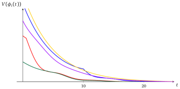
where and denote the two elements of . Following Step 1, item (i) of Corollary 2 holds, since and are satisfied choosing . Since (64) and (65) hold, invoking Proposition 7 we have that item (ii) of Corollary 2 is satisfied, and is a Lyapunov function proving GAS of system (67). In Figure 4, we have plotted the evolution of along 5 particular solutions of system (67).
7 Conclusions
For the class of systems comprising differential inclusions, and state-dependent switched systems, we introduced a family of nonsmooth functions obtained by max-min combinations. Based on two notions of generalized directional derivatives, we proposed sufficient conditions for global asymptotic stability. For a class of systems with conic switching regions and linear dynamics within each of these regions, we studied some conditions under which a max-min condition can be obtained by solving matrix inequalities. A possible route for future research is the generalization of this approach to a wider class of systems, and develop further numerical tools for checking the proposed Lie derivative based conditions.
Appendix A A Technical Lemma
Lemma 4.
Consider invertible and any max-min function , such that satisfy (65). Consider a point such that and (). If , , , for all , then there exists a sequence such that and , for all , for an .
Proof.
Since is invertible, for all such that , we can define the tangent space of at as , see for example [6, Page 23]. Consider , , such that and , for all , . Such a exists, since, by (65), and are invertible and and are linearly independent, for all , . By definition of , given , there exists continuously differentiable function such that , , and , (i.e. ), . For all , , define as
Since we have ; moreover is continuously differentiable at and by the chain rule . This means that there exists a , such that
| (68) |
for all , for all , . We now consider a sequence such that , , and define . Without loss of generality we can suppose , for all , where is the open neighborhood of defined in Lemma 1. By (68) we have
By Lemma 1 this implies that, , there exists such that . By finiteness of , possibly considering a subsequence, we can suppose , with . Since, by definition of , , , we also have , . ∎
References
- [1] A. A. Ahmadi, R. M. Jungers, P. A. Parrilo, and M. Roozbehani. Joint spectral radius and path-complete graph Lyapunov functions. SIAM Journal on Control and Optimization, 52(1):687–717, 2014.
- [2] D. Angeli, N. Athanasopoulos, R. M. Jungers, and M. Philippe. Path-complete graphs and common Lyapunov functions. In Proc. 20th ACM Conf. Hybrid Systems: Computation and Control, pages 81–90, 2017.
- [3] A. Bacciotti and F. M. Ceragioli. Stability and stabilization of discontinuous systems and nonsmooth Lyapunov functions. ESAIM: Control, Optimisation and Calculus of Variations, 4:361–376, 1999.
- [4] A. Bacciotti and L. Rosier. Lyapunov Functions and Stability in Control Theory. Springer-Verlag, Heidelberg, 2nd edition, 2005.
- [5] R. Baier, L. Grüne, and S. F. Hafstein. Linear programming based Lyapunov function computation for differential inclusions. Discrete & Continuous Dynamical Systems - B, 17:33, 2012.
- [6] D. Barden and C. B. Thomas. An Introduction to Differential Manifolds. Imperial College Press, 2003.
- [7] F. Blanchini and S. Miani. Set-Theoretic Methods in Control. Birkhäuser, 2008.
- [8] F. Blanchini and C. Savorgnan. Stabilizability of switched linear systems does not imply the existence of convex Lyapunov functions. Automatica, 44(4):1166–1170, 2008.
- [9] F. M. Ceragioli. Discontinuous ordinary differential equations and stabilization. PhD thesis, Univ. Firenze, Italy, 2000. Available online: http://porto.polito.it/2664870/.
- [10] F. H. Clarke. Optimization and Nonsmooth Analysis. Classics in Applied Mathematics. SIAM, 1990.
- [11] F. H. Clarke, Y. S. Ledyaev, R. J. Stern, and P.R. Wolenski. Nonsmooth Analysis and Control Theory, volume 178 of Graduate Texts in Mathematics. Springer-Verlag, New York, 1998.
- [12] J. Cortes. Discontinuous dynamical systems. IEEE Control Systems Magazine, 28(3):36–73, 2008.
- [13] W. P. Dayawansa and C. F. Martin. A converse Lyapunov theorem for a class of dynamical systems which undergo switching. IEEE Transactions on Automatic Control, 44(4):751–760, 1999.
- [14] R. A. DeCarlo, M. S. Branicky, S. Pettersson, and B. Lennartson. Perspectives and results on the stability and stabilizability of hybrid systems. Proceedings of the IEEE, 88:1069–1082, 2000.
- [15] M. Della Rossa, A. Tanwani, and L. Zaccarian. Max-min Lyapunov functions for switching differential inclusions. In 57th IEEE Conf. on Decision and Control (CDC), pages 5664–5669, 2018.
- [16] A. F. Filippov. Differential Equations with Discontinuous Right-Hand Side. Kluwer Academic Publisher, 1988.
- [17] R. Goebel, T. Hu, and A. R. Teel. Dual matrix inequalities in stability and performance analysis of linear differential/difference inclusions. In Current trends in nonlinear systems and control, pages 103–122. Springer, 2006.
- [18] R. Goebel, R. G. Sanfelice, and A. R. Teel. Hybrid Dynamical Systems: Modeling, Stability, and Robustness. Princeton University Press, 2012.
- [19] R. Goebel, A. R. Teel, T. Hu, and Z. Lin. Conjugate convex Lyapunov functions for dual linear differential inclusions. IEEE Transactions on Automatic Control, 51(4):661–666, 2006.
- [20] T. Hu and F. Blanchini. Non-conservative matrix inequality conditions for stability/stabilizability of linear differential inclusions. Automatica, 46(1):190 – 196, 2010.
- [21] T. Hu, L. Ma, and Z. Lin. Stabilization of switched systems via composite quadratic functions. IEEE Transactions on Automatic Control, 53(11):2571–2585, 2008.
- [22] R. Iervolino, D. Tangredi, and F. Vasca. Lyapunov stability for piecewise affine systems via cone-copositivity. Automatica, 81:22–29, 2017.
- [23] M. Johansson and A. Rantzer. Computation of piecewise quadratic Lyapunov functions for hybrid systems. IEEE Transactions on Automatic Control, 43(4):555–559, 1998.
- [24] R. Kamalapurkar, J.A. Rosenfeld, A. Parikh, A.R. Teel, and W.E. Dixon. Invariance-like results for nonautonomous switched systems. IEEE Transactions on Automatic Control, 64(2):614–627, 2019.
- [25] H. K. Khalil. Nonlinear Systems. Pearson Education. Prentice Hall, 2002.
- [26] D. Liberzon. Switching in Systems and Control. Birkhaüser, 2003.
- [27] D. Liberzon, J. P. Hespanha, and A. S. Morse. Stability of switched systems: A Lie-algebraic condition. Systems & Control Letters, 37:117–122, 1999.
- [28] H. Lin and P.J. Antsaklis. Stability and stabilizability of switched linear systems: A survey of recent results. IEEE Transactions on Automatic Control, 54(2):308 – 322, 2009.
- [29] M. Malisoff and F. Mazenc. Constructions of Strict Lyapunov Functions. Communications and Control Engineering. Springer-Verlag, London, 2009.
- [30] P. Mason, U. Boscain, and Y. Chitour. Common polynomial Lyapunov functions for linear switched systems. SIAM Journal on Optimization and Control, 45(1), 2006.
- [31] A. P. Molchanov and Y. S. Pyatnitskiy. Criteria of asymptotic stability of differential and difference inclusions encountered in control theory. Systems & Control Letters, 13(1):59–64, 1989.
- [32] K. S. Narendra and J. Balakrishnan. A common Lyapunov function for stable LTI systems with commuting -matrices. IEEE Transactions on Automatic Control, 39:2469–2471, 1994.
- [33] S. Ovchinnikov. Discrete piecewise linear functions. European Journal of Combinatorics, 31(5):1283 – 1294, 2010.
- [34] J.-S. Pang and D. Ralph. Piecewise smoothness, local invertibility, and parametric analysis of normal maps. Mathematics of Operations Research, 21(2):401–426, 1996.
- [35] A. Papachristodoulou and S. Prajna. Robust stability analysis of nonlinear hybrid systems. IEEE Transactions on Automatic Control, 54(5):1037–1043, 2009.
- [36] S. Pettersson and B. Lennartson. Hybrid system stability and robustness verification using linear matrix inequalities. International Journal of Control, 75(16-17):1335–1355, 2002.
- [37] S. Scholtes. Introduction to Piecewise Differentiable Equations. Springer Briefs in Optimization. Springer-Verlag, New York, 2012.
- [38] R. Shorten, F. Wirth, O. Mason, K. Wulff, and C. King. Stability criteria for switched and hybrid systems. SIAM Review, 49(4):545–592, 2007.
- [39] A. R. Teel and L. Praly. On assigning the derivative of a disturbance attenuation control Lyapunov function. Mathematics of Controls, Signals, and Systems, 13:95–124, 2000.
- [40] A. R. Teel and L. Praly. A smooth Lyapunov function from a class- estimate involving two positive semidefinite functions. ESAIM: Control, Optimisation and Calculus of Variations, 5:313–367, 2000.
- [41] L. Xie, S. Shishkin, and M. Fu. Piecewise Lyapunov functions for robust stability of linear time-varying systems. Systems & Control Letters, 31(3):165–171, 1997.