A Sliced Wasserstein Loss for Neural Texture Synthesis

Abstract

We address the problem of computing a textural loss based on the statistics extracted from the feature activations of a convolutional neural network optimized for object recognition (VGG-19). The underlying mathematical problem is the measure of the distance between two distributions in feature space. The Gram-matrix loss is the ubiquitous approximation for this problem but it is subject to several shortcomings. Our goal is to promote the Sliced Wasserstein Distance as a replacement for it. It is theoretically proven, practical, simple to implement, and achieves results that are visually superior for texture synthesis by optimization or training generative neural networks.

1 Introduction

A texture is by definition a class of images that share a set of stationary statistics. One of the key components of texture synthesis is a textural loss that measures the difference between two images with respect to these stationary statistics.

Gatys et al. [5] discovered that the feature activations in pretrained Convolutional Neural Networks (CNNs) such as VGG-19 [20] yield powerful textural statistics. Neural texture synthesis means optimizing an image to match the feature distributions of a target texture in each convolutional layer, as shown in Figure 1. Gatys et al.use the $L^{2}$ distance between the Gram matrices of the feature distributions as a textural loss $\mathcal{L}_{\text{Gram}}$. The simplicity and practicability of this loss make it especially attractive and it is nowadays ubiquitous in neural texture synthesis and style transfer methods [6, 4, 23, 14, 24, 11, 21, 19, 27, 26].

input	optim $\mathcal{L}_{\text{Gram}}$	optim $\mathcal{L}_{\text{SW}}$

Figure 1: Neural texture synthesis. We visualize a 2D slice of the feature distributions of a convolutional layer. The ubiquitous Gram-Matrix loss $\mathcal{L}_{\text{Gram}}$ captures only the major directions of the distribution. We promote the Sliced Wasserstein Distance $\mathcal{L}_{\text{SW}}$ that captures the full distribution and allows for neural texture synthesis with improved quality.

Intuitively, the Gram-matrix loss $\mathcal{L}_{\text{Gram}}$, which is a second-order descriptor like the covariance matrix, optimizes the features to be distributed along the same major directions but misses other (higher-order) statistics and is thus insufficient to represent the precise shape of the distribution. This results in undesired artifacts in the synthesized results such as contrast oscillation, as shown in Figure 1-middle. Several subsequent works hint that improved textural quality can be obtained by capturing more statistics [14, 18, 15]. However, how to define a practical textural loss that captures the complete feature distributions remains an open problem.

Our main point is that the classic color transfer algorithm of Pitie et al. [16] provides a simple solution to this problem. This concept is also known as the Sliced Wasserstein Distance (SWD) [17, 1]. It is a slicing algorithm that matches arbitrary n-dimensional (nD) distributions, which is precisely the textural loss problem that the neural texture synthesis community tries to solve. Although it has been around and well-studied for a long time, it surprisingly has not yet been considered for neural texture synthesis and we wish to promote it in this context. In Section 4, we show that the SWD can be transposed to deep feature spaces to obtain a textural loss $\mathcal{L}_{\text{SW}}$ that captures the complete feature distributions and that is practical enough to be considered as a replacement for $\mathcal{L}_{\text{Gram}}$. Furthermore, we show in Section 5 how to account for user-defined spatial constraints without changing $\mathcal{L}_{\text{SW}}$ and without adding further losses or fine-tuned parameters, extending the range of applications reachable with a single textural loss without added complexity.

2 Problem Statement

Our objective is to define a textural loss that captures the complete feature distributions of $L$ target layers of a pretrained convolutional neural network. For our experiments, we use the first $L=12$ convolutional layers of a pretrained VGG-19 with normalized weights, following Gatys et al. [5].

Notations.

The convolutional layer $l$ has $M_{l}$ pixels (spatial dimensions) and $N_{l}$ features (depth dimension). We note $F^{l}_{m}\in\mathbb{R}^{N_{l}}$ the feature vector located at pixel $m$ and $F^{l}_{m}[n]\in\mathbb{R}$ its n-th component ($n<N_{l})$.

Deep feature distributions.

We note $p_{l}$ the probability density function of the features in layer $l$. Since the feature activations are discrete in a convolutional neural network, the density is a sum of delta Dirac distributions

$$p^{l}(x)=\frac{1}{M_{l}}\,\sum_{m=1}^{M_{l}}\delta_{F^{l}_{m}}(x)$$ (1)

that can be visualized as a point cloud in feature space (Figure 1). These distributions are position-agnostic, they do not depend on where the features are located in image space, and provide a stationary statistic of the texture.

Textural loss.

A textural loss between two images $I$ and $\tilde{I}$ is a function $\mathcal{L}(I,\tilde{I})\in\mathbb{R}^{+}$ that measures a distance between the sets of distributions $p^{l}$ and $\tilde{p}^{l}$ associated with the images.

Objective.

Our goal is to define a textural loss that captures full feature distributions,

$$\mathcal{L}(I,\tilde{I})=0\implies p^{l}=\tilde{p}^{l}~{}~{}\forall~{}l\in\{1,..,L\}.$$ (2)

Furthermore, this loss should be practical enough to be used for texture optimization or training generative networks.

3 Previous work

The Gram loss.

Gatys et al. [5, 6] use the Gram matrices of the feature distributions to define a textural loss:

$$\mathcal{L}_{\tiny\text{Gram}}(I,\tilde{I}) =\sum_{l=1}^{L}\frac{1}{N^{2}_{l}}\,\left\|G^{l}-\tilde{G}^{l}\right\|^{2},$$ (3)

where $G^{l}$ (resp. $\tilde{G}^{l}$) is the Gram matrix of the deep features extracted from $I$ (resp. $\tilde{I}$) at layer $l$. $G_{ij}^{l}$ is the entry $(i,j)$ of the Gram matrix $G^{l}\in\mathbb{R}^{N_{l}\times N_{l}}$ of layer $l$, defined as the second-order cross-moment of features $i$ and $j$ over the pixels:

$$G_{ij}^{l} =\mathbb{E}\left[F^{l}_{m}[i]\,F^{l}_{m}[j]\right]=\frac{1}{M^{l}}\,\sum_{m}F^{l}_{m}[i]\,F^{l}_{m}[j].$$ (4)

The Gram loss has become ubiquitous as a textural loss because it is fast to compute and practical. However, it does not capture the full distribution of features,

$$\mathcal{L}_{\tiny\text{Gram}}(I,\tilde{I})=0\centernot\implies p^{l}=\tilde{p}^{l}~{}~{}\forall~{}l\in\{1,..,L\}.$$ (5)

This explains the visual artifacts of Figure 1-middle.

Beyond the Gram loss.

Many have noticed that $\mathcal{L}_{\text{Gram}}$ does not capture every aspect of appearance, resulting in artifacts [14, 13, 18, 21, 19, 15, 27, 26]. Some approaches switch paradigm by training Generative Adverserial Networks (GANs) but this is out of the scope of the problem defined in Section 2 that is the focus of this article.

The closest approach to ours is the one of Risser et al. [18] who define a histogram loss $\mathcal{L}_{\tiny\text{Hist}}$ by adding the sum of the 1D axis-aligned histogram losses of each of the $N_{l}$ features to the Gram loss:

$$\mathcal{L}_{\tiny\text{Hist}}(I,\tilde{I})=\sum_{l=1}^{L}\sum_{n=1}^{N_{l}}\mathcal{L}_{\tiny\text{Hist1D}}(p^{l}_{n},\tilde{p}^{l}_{n})+\alpha\,\mathcal{L}_{\tiny\text{Gram}}(I,\tilde{I}).$$ (6)

This loss does not capture all the stationary statistics:

$$\mathcal{L}_{\tiny\text{Hist}}(I,\tilde{I})=0\centernot\implies p^{l}=\tilde{p}^{l}~{}~{}\forall~{}l\in\{1,..,L\},$$ (7)

but significantly improves the results in comparison to $\mathcal{L}_{\text{Gram}}$, hinting that capturing more statistics improves textural quality. In terms of practicability, a careful tuning of its relative weight is required. Moreover, each 1D histogram loss $\mathcal{L}_{\tiny\text{Hist1D}}$ uses a histogram binning. The number of bins is yet another sensitive parameter to tune: insufficient bins result in poor accuracy while the opposite results in vanishing gradient problems. Our Sliced Wasserstein loss also computes 1D losses but with an optimal transport formulation (implemented by a sort) rather than a binning scheme and with arbitrary rather than axis-aligned directions, which makes it statistically complete, simpler to use, and allows to get rid of the Gram loss and its weighting parameter.

Other approaches were designed inspired by the idea of capturing the full distribution of features. Mechrez et al.’s contextual loss $\mathcal{L}_{\text{CX}}$ [15] estimates the difference between two distributions and resembles Li and Malik’s implicit maximum likelihood estimator [10]. Unfortunately, it uses a kernel with an extra meta-parameter $h$ to tune and has a quadratic complexity, severely limiting its usability. Another recent work is Kolkin et al.’s approximate earth mover’s distance loss $\mathcal{L}_{\text{REMD}}$ [8]. It requires several regularization terms with fine-tuned weights. These losses are still not complete:

$$\mathcal{L}_{\tiny\text{CX}}(I,\tilde{I})=0\centernot\implies p^{l}=\tilde{p}^{l}~{}~{}\forall~{}l\in\{1,..,L\},$$ (8)

$$\mathcal{L}_{\tiny\text{REMD}}(I,\tilde{I})=0\centernot\implies p^{l}=\tilde{p}^{l}~{}~{}\forall~{}l\in\{1,..,L\},$$ (9)

and are not good candidates for the texture synthesis application for which they achieve textural quality even inferior to a vanilla $\mathcal{L}_{\text{Gram}}$. We further discuss the problems arising when using $\mathcal{L}_{\text{CX}}$ and $\mathcal{L}_{\text{REMD}}$ for texture synthesis in Appendix A. To our knowledge, a loss that is proven to capture the full distribution of features and provides a practical candidate for texture synthesis has not been proposed yet. We believe that the Sliced Wasserstein Distance is the right candidate for this problem.

The Sliced Wasserstein Distance.

Our main source of inspiration is the color transfer algorithm of Pitie et al. [16]. They show that iteratively matching random 1D marginals of an n-Dimensional distribution is a sufficient condition to converge towards the distribution, satisfying Equation (2). This idea has been applied in the context of optimal transport [17, 1]: distances between distributions can be measured with the Wasserstein Distance and the expectation over random 1D marginals provides a practical approximation that scales in $\mathcal{O}(n\log{}n)$. Note that it is approximate in the sense that the optimized transport map is not optimal but the optimized distribution is proven to converge towards the target distribution, it satisfies Equation (2). The Sliced Wasserstein Distance allows for fast gradient descent algorithms and is suitable for training generative neural networks [9, 3, 25]. It has also been successfully used for texture synthesis by gradient descent using wavelets as a feature extractor [22]. By using a pretrained CNN as a feature extractor [5], we bring this proven and practical solution to neural texture synthesis and solve the problem defined in Section 2.

Neural texture synthesis with spatial constraints.

The problem defined in Section 2 aims at capturing the stationary statistics that define a texture. For some applications, additional non-stationary spatial constraints are required. The mainstream way to handle spatial constraints in neural texture synthesis is to combine $\mathcal{L}_{\text{Gram}}$ with additional losses [2, 14, 19, 27]. For example: Liu et al.add a loss on the power spectrum of the texture so as to preserve the frequency information [14]; Sendik and Cohen-Or [19] add a loss function capturing deep feature correlations with shifted versions of themselves, which makes the optimisation at least an order of magnitude slower. All those losses require tuning of both inter-loss weights and inter-layer weights within each loss. Champandard [2] proposes to concatenate user-defined guidance maps to the deep features prior to extracting statistics. Gatys et al. [7] show that this hinders textural quality and propose a more qualitative but slower per-cluster variant, which duplicates computation per tag, disallowing numerous tags. Both methods have sensitive parameters to fine-tune. In Section 5, we show how to handle user-defined spatial constraints without modifying the Sliced Wasserstein loss nor adding further losses or compromising complexity.

4 The Sliced Wasserstein Loss

In this section, we show how to compute a neural loss with the Sliced Wasserstein Distance [16, 9, 3, 25] and we note it $\mathcal{L}_{\tiny\text{SW}}$.

Figure 2: The Sliced Wasserstein loss. We project n-dimensional features onto random directions, sort the 1D projections, and compute the $L^{2}$ difference between the sorted lists.

Definition.

We define the Sliced Wasserstein loss as the sum over the layers:

$$\mathcal{L}_{\tiny\text{SW}}(I,\tilde{I})=\sum_{l=1}^{L}\mathcal{L}_{\tiny\text{SW}}(p^{l},\tilde{p}^{l}).$$ (10)

where $\mathcal{L}_{\tiny\text{SW}}(p^{l},\tilde{p}^{l})$ is a Sliced Wasserstein Distance between the distribution of features $p^{l}$ and $\tilde{p}^{l}$ of layer $l$. It is the expectation of the 1D optimal transport distances after projecting the feature points onto random directions $V\in\mathcal{S}^{N_{l}}$ on the unit n-dimensional hypersphere of features:

$$\mathcal{L}_{\text{SW}}(p_{l},\tilde{p}_{l})=\mathbb{E}_{V}[\mathcal{L}_{\tiny\text{SW1D}}(p_{V}^{l},\tilde{p}_{V}^{l})],$$ (11)

where $p_{V}^{l}=\{\langle F_{m}^{l},V\rangle\},\forall m$ is the unordered scalar set of dot products between the $m$ feature vectors $F_{m}^{l}$ and the direction $V$. $\mathcal{L}_{\tiny\text{SW1D}}$ is the 1D optimal transport loss between two unordered set of scalars. It is defined as the element-wise $L^{2}$ distance over sorted lists:

$$\mathcal{L}_{\text{SW1D}}(S,\tilde{S})=\frac{1}{|S|}\,\left\|\text{sort}(S)-\text{sort}(\tilde{S})\right\|^{2}.$$ (12)

We illustrate the projection, sorting and distance between $p_{V}^{l}$ and $\tilde{p}_{V}^{l}$ in Figure 2.

Properties.

Pitie et al. [16] prove that the SWD captures the complete target distribution,

$$\mathcal{L}_{\tiny\text{SW}}(p^{l},\tilde{p}^{l})=0\implies p^{l}=\tilde{p}^{l}.$$ (13)

It follows that it satisfies the implication of Eq. (2):

$$\mathcal{L}_{\tiny\text{SW}}(I,\tilde{I})=0\implies p^{l}=\tilde{p}^{l}~{}~{}\forall~{}l\in\{1,..,L\},$$ (14)

and hence solves the problem targeted in this paper (Sec. 2).

Because the loss $\mathcal{L}_{\text{SW}}$ captures the complete stationary statistics of deep features, it achieves the upperbound of what can be extracted as a stationary statistic from the layers of a given convolutional neural network. For instance, it encompasses $\mathcal{L}_{\text{Gram}}$ [5], $\mathcal{L}_{\tiny\text{Hist}}$ [18], $\mathcal{L}_{\text{CX}}$ [15] and $\mathcal{L}_{\text{REMD}}$ [8]:

$$\mathcal{L}_{\tiny\text{SW}}(I,\tilde{I})=0 \implies\mathcal{L}_{\tiny\text{Gram}}(I,\tilde{I})=0,$$ (15)

$$\mathcal{L}_{\tiny\text{SW}}(I,\tilde{I})=0 \implies\mathcal{L}_{\tiny\text{Hist}}(I,\tilde{I})=0,$$ (16)

$$\mathcal{L}_{\tiny\text{SW}}(I,\tilde{I})=0 \implies\mathcal{L}_{\tiny\text{CX}}(I,\tilde{I})=0,$$ (17)

$$\mathcal{L}_{\tiny\text{SW}}(I,\tilde{I})=0 \implies\mathcal{L}_{\tiny\text{REMD}}(I,\tilde{I})=0$$ (18)

Figure 3 shows experimentally that optimizing for $\mathcal{L}_{\text{SW}}$ also optimizes for $\mathcal{L}_{\text{Gram}}$ while the opposite is not true.

Figure 3: Loss curves for the images of Figure 5. Optimizing for $\mathcal{L}_{\text{Gram}}$ (blue) or $\mathcal{L}_{\text{SW}}$ (red). We monitor the evolution of the values of $\mathcal{L}_{\text{Gram}}$ (left) and $\mathcal{L}_{\text{SW}}$ (right) in either case. $\mathcal{L}_{\text{SW}}$ encompasses $\mathcal{L}_{\text{Gram}}$: minimizing $\mathcal{L}_{\text{SW}}$ minimizes $\mathcal{L}_{\text{Gram}}$ but the opposite is not true.

Implementation.

Listing 1 shows that it boils down to projecting the features on random directions (unit vectors of dimension $N_{l}$), sort the projections and measure the $L^{2}$ distance on the sorted lists. Because it computes a $L^{2}$ distance on a sorted list, this loss is differentiable everywhere and can be used for gradient retropropagation. Furthermore, Tensorflow and Pytorch both provide an efficient GPU implementation of the sort() function. To create images $n$ times larger than the example, we simply repeat each entry $n$ times in the latter’s sorted list when evaluating the loss.

⬇

# slicing

Vs = random_directions()

def Slicing(F):

# project each pixel feature onto directions

proj = dot(F, Vs)

# flatten pixel indices to [M,N]

H, W, N = proj.shape

proj_flatten = reshape(proj,(H*W,N))

# sort projections for each direction

return sort(proj_flatten, axis=0)

# Sliced Wasserstein loss between two layers

def SlicedWassersteinLoss(F, F_):

diff = Slicing(F) - Slicing(F_)

return mean(square(diff))

Listing 1: Implementation of the Sliced Wasserstein loss. The variable Vs is a matrix whose columns are normalized random directions in feature space. Random directions are redrawn for each batch.

Number of random directions.

Iterating over random directions makes $\mathcal{L}_{\text{SW}}$ converge towards the target distribution regardless of the number of directions. However, this number has an effect analogous to the batch size for stochastic gradient descent: it influences the noise in the gradient. In Figure 4, we compare convergence (monitored as $\mathcal{L}_{\text{SW}}$ with many directions) of optimisations that use different numbers of directions. A low number is faster to compute and uses less memory but is slower to converge due to noisy gradients. A high number requires more computation and memory but generates less noisy gradients thus converges faster. In practice, we use $N_{l}$ random directions, as many as there are features in layer $l$. In this setting, we note an increased computational cost of $\approx 1.7-2.8\times$ over $\mathcal{L}_{\text{Gram}}$.

Figure 4: Number of random directions. We compare convergence (left, texture size $256^{2}$) and runtime (right, various sizes, 10 steps) of optimizing $\mathcal{L}_{\text{SW}}$ with a varying number of directions. Setting: SciPy’s L-BFGS-B ($maxfun=64,pgtol=0.0,factr=0.0$) in Python and Tensorflow 2.3 on Intel Core i5 and NVidia Titan Xp.

Texture synthesis by optimization.

In Figure 5, we compare $\mathcal{L}_{\text{SW}}$ to $\mathcal{L}_{\text{Gram}}$ in the scope of iterative texture optimization with an L-BFGS-B optimizer. This setting is the right unit test to validate the textural loss that drives the optimization, avoiding issues related to training neural networks or meta-parameter tuning. We observe that $\mathcal{L}_{\text{Gram}}$ produces artifacts such as oscillating contrasts and is inconsistent different input sizes (last row), making it less predictable. These limitations of $\mathcal{L}_{\text{Gram}}$ are documented in previous works [18, 19]. In contrast, $\mathcal{L}_{\text{SW}}$ generates uniformly sharp textures consistent different input sizes. Figure 6 confirms these observations with style transfer.

Training generative neural networks.

While direct texture optimization is a good unit test for the loss, we also validate that we can successfully use $\mathcal{L}_{\text{SW}}$ for training. In Figure 7 and 8 we use $\mathcal{L}_{\text{SW}}$ for sole loss function to train a mono-texture [23] and a multi-texture [12] generative architecture, respectively. They are capable of producing arbitrarily-large texture at inference time, with variation (no verbatim copying of the exemplar) and interpolation. This experiment validates that there are a priori no obstacles to using $\mathcal{L}_{\text{SW}}$ as a drop-in replacement for $\mathcal{L}_{\text{Gram}}$ for training.

	optim $\mathcal{L}_{\text{Gram}}$ $512\times 512$	optim $\mathcal{L}_{\text{SW}}$ $512\times 512$		optim $\mathcal{L}_{\text{Gram}}$ $512\times 512$	optim $\mathcal{L}_{\text{SW}}$ $512\times 512$
input $128\times 128$			input $256\times 256$
input $128\times 128$			input $256\times 256$
input $128\times 128$			input $256\times 256$

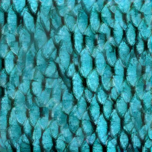
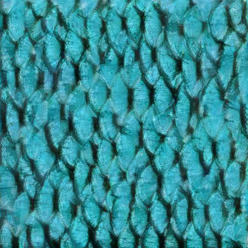
Figure 5: Texture synthesis by optimization. We optimize a Gaussian white noise with $\mathcal{L}_{\text{Gram}}$ and $\mathcal{L}_{\text{SW}}$ using L-BGFS. In the last row, the inputs are two crops of different sizes extracted from the same texture.

Content	Style	optim $\mathcal{L}_{\text{Gram}}$	optim $\mathcal{L}_{\text{SW}}$	Style	optim $\mathcal{L}_{\text{Gram}}$	optim $\mathcal{L}_{\text{SW}}$
$512\times 512$	$128\times 128$	$512\times 512$	$512\times 512$	$256\times 256$	$512\times 512$	$512\times 512$

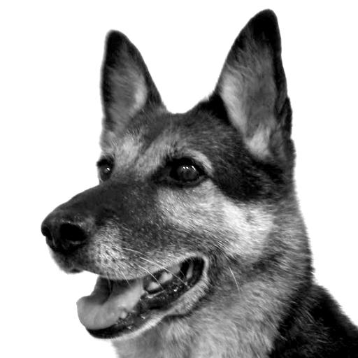
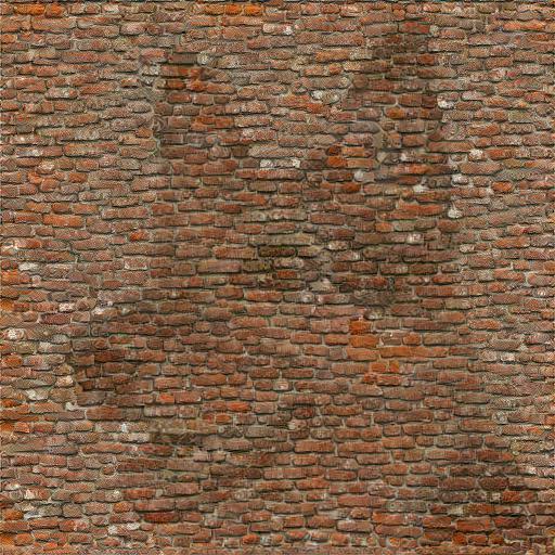
Figure 6: Style transfer by optimization. We optimize the content image with $\mathcal{L}_{\text{Gram}}$ and $\mathcal{L}_{\text{SW}}$ using L-BGFS (we do not add a content loss with a tuneable parameter such as [6]).

example	generated	example	generated	example	generated

Figure 7: Training a mono-texture generator. We use $\mathcal{L}_{\text{SW}}$ to train a mono-texture generative architecture [23].

example 1	generated	example 2	example 3	generated	example 4

Figure 8: Training a multi-texture generator. We use $\mathcal{L}_{\text{SW}}$ to train a multi-texture generative architecture that allows for interpolation [12]. We trained the same architecture for 32 textures that includes these 4 examples.

5 Spatial Constraints Via User-Defined Tags

The Sliced Wasserstein loss $\mathcal{L}_{\text{SW}}$ presented in Section 4 captures all the stationary, position-agnostic, statistics. Like the Gram loss, it means that one has no spatial control over the synthesized textures that are optimized with this loss. For some applications where spatial constraints are required, previous works usually use additional losses whose relative weighting has to be fine-tuned. In this section, we propose a simple way to incorporate spatial constraints in the Sliced Wasserstein loss $\mathcal{L}_{\text{SW}}$ without any modification and without adding further losses.

Figure 9: Spatial constraints via user-defined tags. The distribution of features does not encode their spatial organization. In this example, $\mathcal{L}_{\text{SW}}$ cannot reproduce a checker pattern in image space (top). Our trick consists in adding a spatial tag that acts like an additional dimension to the feature space. With this new dimension, the feature distribution can represent spatial structures that are processed by $\mathcal{L}_{\text{SW}}$ like any other feature space dimension (bottom).

Non-stationary statistics.

Figure 9-top illustrates the case of feature activations that are organized like a checkerboard in image space. Since the feature distribution is independent of the image-space locations of the features, optimizing the feature distribution does not preserve the checkerboard pattern.

Spatial constraints via user-defined tags.

Our idea is to introduce spatial information in the feature distribution by adding a new dimension to the feature space that stores a spatial tag. In Figure 9-bottom, the 2D feature space becomes 3D and the third dimension stores a binary tag that encodes the checker pattern such that the only way for the optimized feature distribution to match the input distribution is to represent a checkerboard. This trick allows for adding spatial constraints that can be provided by user-defined spatial tags. Note that the spatial tags are fixed, they cannot be optimized, and they need to have the same distribution in the input and the output.

Homogeneity of the loss.

An important point is to add the spatial dimension without breaking the homogeneity of the feature space loss $\mathcal{L}_{\text{SW}}$. To do this, we concatenate spatial tags to the feature vectors $\left(F^{l}_{m}[1],..,F^{l}_{m}[N^{l}],\text{tag}\right)$, concatenate 1 to the normalized projection direction in feature space $\left(V_{1},..,V_{N^{l}},1\right)$, and optimize for $\mathcal{L}_{\text{SW}}$ without further modifications. We use spatial tags that are strictly larger than the other dimensions in feature space such that the sorting in $\mathcal{L}_{\text{SW}}$ groups the pixels in clusters that have the same tag. As a result, the tags only change the sorting order and vanish after subtraction in Equation (12). The introduction of the spatial dimension thus does not break the homogeneity of $\mathcal{L}_{\text{SW}}$ that remains a feature-space $L^{2}$ between sorted features. No additional loss and no meta-parameter tuning is required with this approach. Note that it is equivalent to solving separate $nD$ histogram losses for each cluster but it is more practical since it requires no more than a concatenation.

Results and positioning.

Figures 10, 11 and 12 show textures optimized with an L-BFGS-B optimizer and with spatial tags concatenated only to the first two layers of VGG-19. Note that we do not aim at comparing the visual quality with competitor works. Our point is to show that $\mathcal{L}_{\text{SW}}$ significantly widens the range of applications reachable with a single textural loss and no meta-parameter tuning.

Painting by texture.

Figure 10 is an example of painting by texture where the user provides a target non-stationary example image, a spatial tag mask associated with the example, and a target spatial tag mask. By optimizing $\mathcal{L}_{\text{SW}}$ with the spatial tags, we obtain a new image that has the same style as the example image but whose large-scale structure follows the desired tag mask. Typically, methods based on neural texture synthesis require parameter fine-tuning and/or an evaluation of the loss term for each tag (cf. our discussion in Section 3). In comparison, $\mathcal{L}_{\text{SW}}$ works out of the box without any tuning and in a single evaluation regardless of the number of different of tags.

Pseudo-periodic patterns.

Figures 11 and 12 focus on textures with an obvious pseudo-period, which is provided as a spatial tag mask (the tag is the pixel coordinates modulo the period) and we optimize with $\mathcal{L}_{\text{SW}}$. The results exhibit the structural regularity of the exemplar at that period, allowing for reproduction of regular textures with stochastic variation in all other frequencies. In Figure 12, our results are comparable to Sendik and Cohen-Or [19] for this class of textures. Note that their method does not require user inputs but is significantly more elaborated and less efficient even for this simple class of textures. It uses $\mathcal{L}_{\text{Gram}}$ in addition to three other losses whose weights need to be fine-tuned. Optimizing $\mathcal{L}_{\text{SW}}$ provides a simpler and efficient solution for this class of textures.

input + tag	optim with tag $\mathcal{L}_{\text{SW}}$

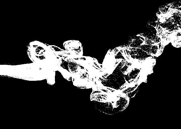
Figure 10: Texture synthesis with spatial constraints: painting by texture. $\mathcal{L}_{\text{SW}}$ accounts for spatial tags concatenated to the deep features.

Figure 11: Texture synthesis with spatial constraints: pseudo-periodic patterns. $\mathcal{L}_{\text{SW}}$ accounts for spatial tags concatenated to the deep features.

Input	Gatys et al.	Sendik et al.	Ours
	$\mathcal{L}_{\text{Gram}}$	$\alpha\mathcal{L}_{\scriptsize\text{Gram}}+\beta\mathcal{L}_{\scriptsize\text{DC}}+$	$\mathcal{L}_{\text{SW}}$ with tag
		$\gamma\mathcal{L}_{\scriptsize\text{Div}}+\delta\mathcal{L}_{\scriptsize\text{S}}$

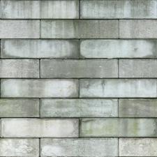
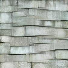
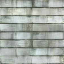
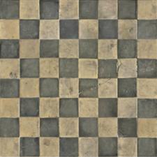
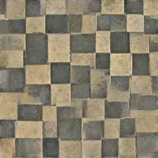
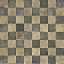
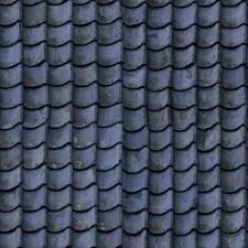
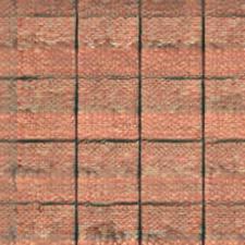
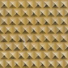
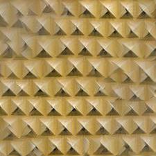
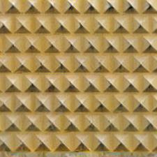
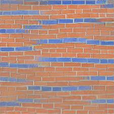
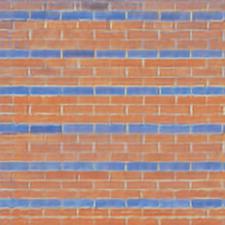
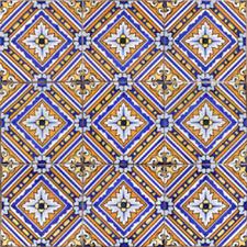
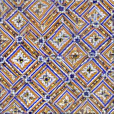
Figure 12: Texture synthesis with spatial constraints: pseudo-periodic patterns. Comparison against Sendik and Cohen-Or’s deep correlation method [19]. We extracted all the inputs and their results from their paper. Our method uses spatial tags that encode the obvious pseudo-period such as in Figure 11.

6 Conclusion

Our objective was to find a robust and high-quality textural loss. Several previous works show that the community felt that capturing the full feature distribution is the right approach for this problem. However, existing approaches are subject to different shortcomings such as quadratic complexity, additional regularization terms, etc. Surprisingly, there existed a much simpler solution from the start in the optimal transport community. The Sliced Wasserstein Distance provides a textural loss with proven convergence, sub-quadratic complexity, simple implementation and that achieves high-quality without further regularization losses. It seems to be the right tool for this problem and we are not aware of any alternative that brings all these qualities together. We benchmarked and validated it in a texture optimization framework, which we believe is the correct way to unit test and validate a textural loss: the results reflect the performance and expressiveness of the loss without being hindered by a generative architecture. Nonetheless, we have also shown that one can successfully use it to train a generative architecture. Finally, we have shown a simple way to handle spatial constraints that widens the expressiveness of the loss without compromising its simplicity, which is, to our knowledge, not possible with the Gram-matrix loss and other alternatives. With these good properties, we hope that the Sliced Wasserstein Distance will be considered as a serious competitor for the Gram-matrix loss in terms of practical adoption for both education, research and production.

Appendix A On Texture Synthesis vs. Style Transfer

In this section, we show that style-transfer methods should not be expected to perform well on texture synthesis unless they are proven to do so. For instance, the textural losses $\mathcal{L}_{\text{CX}}$ by Mechrez et al. [15] and $\mathcal{L}_{\text{REMD}}$ by Kolkin et al. [8] are state-of-the-art for style transfer but, in our experience, they perform worse than a vanilla $\mathcal{L}_{\text{Gram}}$ when used for pure texture synthesis. The right ablation study to evaluate texture quality is texture synthesis, not style transfer in which other effects are mixed in. To support this point, we took the implementations of $\mathcal{L}_{\text{CX}}$ and $\mathcal{L}_{\text{REMD}}$ provided by their authors and adapted them to texture synthesis.

In Figure 13, we show a texture synthesis experiment with the implementation of $\mathcal{L}_{\text{CX}}$ provided by Mechrez et al. [15] (in which we disabled the content loss). The memory allocator crashes beyond a resolution of $100^{2}$ due to $\mathcal{O}(n^{2})$ complexity (they limit to $65^{2}$) and the results are visually worse than with $\mathcal{L}_{\text{Gram}}$ (we tried several values for their $h$ parameter and kept the best results).

In Figure 14, we show a texture synthesis experiment with the implementation of $\mathcal{L}_{\text{REMD}}$ provided by Kolkin et al. [8] on a texture extracted from their paper (again, we disabled content loss). The result is qualitatively worse than with $\mathcal{L}_{\text{Gram}}$. Furthermore, $\mathcal{L}_{\text{REMD}}$ needs two additional regularization losses ($\mathcal{L}_{\text{m}}$ and $\mathcal{L}_{\text{p}}$) without which quality decreases significantly.

From these experiments, we conclude that $\mathcal{L}_{\text{CX}}$ and $\mathcal{L}_{\text{REMD}}$ are not good candidates for texture synthesis and that, more generally, state-of-the-art style transfer methods are not necessarily good candidates for texture synthesis.

Input	$\mathcal{L}_{\text{Gram}}$	$\mathcal{L}_{\text{CX}}$
$100\times 100$	$100\times 100$	$100\times 100$

Figure 13: Texture optimization using $\mathcal{L}_{\text{CX}}$ [15]. Results are limited to a resolution of $100\times 100$ and are of low quality.

Input	$\mathcal{L}_{\text{Gram}}$
$256\times 256$	$512\times 512$
$\mathcal{L}_{\text{REMD}}$ + $\mathcal{L}_{\text{m}}$ + $\mathcal{L}_{\text{p}}$	$\mathcal{L}_{\text{REMD}}$
$512\times 512$	$512\times 512$

Figure 14: Texture optimization using $\mathcal{L}_{\text{REMD}}$ [8]. The loss achieves poor textural quality by itself. The textural quality remains inferior to $\mathcal{L}_{\text{Gram}}$ even when using the proposed additional regularization losses $\mathcal{L}_{\text{m}}$ and $\mathcal{L}_{\text{p}}$.

References

- [1] Nicolas Bonneel, Julien Rabin, Gabriel Peyré, and Hanspeter Pfister. Sliced and radon wasserstein barycenters of measures. J. Math. Imaging Vis., 51(1):22–45, 2015.
- [2] Alex J. Champandard. Semantic style transfer and turning two-bit doodles into fine artworks. CoRR, abs/1603.01768, 2016.
- [3] Ishan Deshpande, Ziyu Zhang, and Alexander G. Schwing. Generative modeling using the sliced wasserstein distance. In The IEEE Conference on Computer Vision and Pattern Recognition (CVPR), June 2018.
- [4] L. A. Gatys, M. Bethge, A. Hertzmann, and E. Shechtman. Preserving color in neural artistic style transfer. Technical report, Bethge Lab, Jun 2016.
- [5] Leon A. Gatys, Alexander S. Ecker, and Matthias Bethge. Texture synthesis using convolutional neural networks. In Proceedings of the 28th International Conference on Neural Information Processing Systems - Volume 1, NIPS’15, page 262–270, Cambridge, MA, USA, 2015. MIT Press.
- [6] Leon A. Gatys, Alexander S. Ecker, and Matthias Bethge. Image style transfer using convolutional neural networks. In The IEEE Conference on Computer Vision and Pattern Recognition (CVPR), June 2016.
- [7] Leon A. Gatys, Alexander S. Ecker, Matthias Bethge, Aaron Hertzmann, and Eli Shechtman. Controlling perceptual factors in neural style transfer. In Proceedings of the IEEE Conference on Computer Vision and Pattern Recognition (CVPR), July 2017.
- [8] Nicholas Kolkin, Jason Salavon, and Gregory Shakhnarovich. Style transfer by relaxed optimal transport and self-similarity. In Proceedings of the IEEE/CVF Conference on Computer Vision and Pattern Recognition (CVPR), June 2019.
- [9] Soheil Kolouri, Charles E. Martin, and Gustavo K. Rohde. Sliced-wasserstein autoencoder: An embarrassingly simple generative model. CoRR, abs/1804.01947, 2018.
- [10] Ke Li and Jitendra Malik. Implicit maximum likelihood estimation. ArXiv, abs/1809.09087, 2018.
- [11] Y. Li, C. Fang, J. Yang, Z. Wang, X. Lu, and M. Yang. Diversified texture synthesis with feed-forward networks. In 2017 IEEE Conference on Computer Vision and Pattern Recognition (CVPR), pages 266–274, 2017.
- [12] Yijun Li, Chen Fang, Jimei Yang, Zhaowen Wang, Xin Lu, and Ming Hsuan Yang. Diversified texture synthesis with feed-forward networks. In Proceedings - 30th IEEE Conference on Computer Vision and Pattern Recognition, CVPR 2017, pages 266–274, 2017.
- [13] Yijun Li, Chen Fang, Jimei Yang, Zhaowen Wang, Xin Lu, and Ming-Hsuan Yang. Universal style transfer via feature transforms. In Proceedings of the 31st International Conference on Neural Information Processing Systems, NIPS’17, page 385–395, Red Hook, NY, USA, 2017. Curran Associates Inc.
- [14] Gang Liu, Yann Gousseau, and Gui-Song Xia. Texture synthesis through convolutional neural networks and spectrum constraints. In 23rd International Conference on Pattern Recognition, ICPR 2016, Cancún, Mexico, December 4-8, 2016, pages 3234–3239. IEEE, 2016.
- [15] Roey Mechrez, Itamar Talmi, and Lihi Zelnik-Manor. The contextual loss for image transformation with non-aligned data. arXiv preprint arXiv:1803.02077, 2018.
- [16] F. Pitie, A. C. Kokaram, and R. Dahyot. N-dimensional probability density function transfer and its application to color transfer. In Tenth IEEE International Conference on Computer Vision (ICCV’05) Volume 1, volume 2, pages 1434–1439 Vol. 2, 2005.
- [17] Julien Rabin, Gabriel Peyré, Julie Delon, and Marc Bernot. Wasserstein barycenter and its application to texture mixing. In Scale Space and Variational Methods in Computer Vision, pages 435–446, 2012.
- [18] Eric Risser, Pierre Wilmot, and Connelly Barnes. Stable and controllable neural texture synthesis and style transfer using histogram losses. CoRR, abs/1701.08893, 2017.
- [19] Omry Sendik and Daniel Cohen-Or. Deep correlations for texture synthesis. ACM Trans. Graph., 36(4), July 2017.
- [20] Karen Simonyan and Andrew Zisserman. Very deep convolutional networks for large-scale image recognition. In International Conference on Learning Representations, 2015.
- [21] Xavier Snelgrove. High-resolution multi-scale neural texture synthesis. In SIGGRAPH Asia 2017 Technical Briefs, SA ’17, New York, NY, USA, 2017. Association for Computing Machinery.
- [22] Guillaume Tartavel, Gabriel Peyré, and Yann Gousseau. Wasserstein loss for image synthesis and restoration. SIAM Journal on Imaging Sciences, 9(4):1726–1755, 2016.
- [23] Dmitry Ulyanov, Vadim Lebedev, Andrea Vedaldi, and Victor Lempitsky. Texture networks: Feed-forward synthesis of textures and stylized images. In Proceedings of the 33rd International Conference on International Conference on Machine Learning - Volume 48, ICML’16, page 1349–1357. JMLR.org, 2016.
- [24] Dmitry Ulyanov, Andrea Vedaldi, and Victor S. Lempitsky. Improved texture networks: Maximizing quality and diversity in feed-forward stylization and texture synthesis. In 2017 IEEE Conference on Computer Vision and Pattern Recognition, CVPR 2017, Honolulu, HI, USA, July 21-26, 2017, pages 4105–4113. IEEE Computer Society, 2017.
- [25] Jiqing Wu, Zhiwu Huang, Dinesh Acharya, Wen Li, Janine Thoma, Danda Pani Paudel, and Luc Van Gool. Sliced wasserstein generative models. In The IEEE Conference on Computer Vision and Pattern Recognition (CVPR), 2019.
- [26] Ning Yu, Connelly Barnes, Eli Shechtman, Sohrab Amirghodsi, and Michal Lukac. Texture mixer: A network for controllable synthesis and interpolation of texture. In The IEEE Conference on Computer Vision and Pattern Recognition (CVPR), June 2019.
- [27] Yang Zhou, Zhen Zhu, Xiang Bai, Dani Lischinski, Daniel Cohen-Or, and Hui Huang. Non-stationary texture synthesis by adversarial expansion. ACM Trans. Graph., 37(4), July 2018.