Monte Carlo Simulation Techniques

Abstract

Monte Carlo simulations are widely used in many areas including particle accelerators. In this lecture, after a short introduction and reviewing of some statistical backgrounds, we will discuss methods such as direct inversion, rejection method, and Markov chain Monte Carlo to sample a probability distribution function, and methods for variance reduction to evaluate numerical integrals using the Monte Carlo simulation. We will also briefly introduce the quasi-Monte Carlo sampling at the end of this lecture.

0.1 Introduction

The Monte Carlo method is a (computational) method that relies on the use of random sampling and probability statistics to obtain numerical results for solving deterministic or probabilistic problems. It is a method of solving various problems in computational mathematics by constructing for each problem a random process with parameters equal to the required quantities of that problem. The unknowns are determined approximately by carrying out observations on the random process and by computing its statistical characteristics which are approximately equal to the required parameters [1].

It is believed that the earliest documented use of random sampling to solve a mathematical problem is by mathematician Comte de Buffon of France in 1777 [2]. This problem is to find the probability of an intersection between a randomly thrown needle of length L and a group of parallel lines with separation width D. It turns out that the analytical solution of this probability is proportional to $\pi$ and later suggested by Laplace to evaluate the $\pi$ using the random sampling. Lord Kelvin used random sampling to aid in evaluating the time integrals associated with the kinetic theory of gases and Enrico Fermi was among the first to apply random sampling methods to study neutron moderation in Rome. During World War II, Fermi, Stan Frankel, Nicholas Metropolis, John von Neumann, Stan Ulam and others developed computer-oriented Monte Carlo methods at Los Alamos to study neutron transport through materials under the Manhattan project. It is said that the name of "Monte Carlo" which is also a casino center for gambling in Monaco, was coined by Metropolis because of the similarity of the randomness employed in the method and games of chance [3].

The Monte Carlo simulation starts with a probability distribution function that characterizes the parameters of the physical or mathematical system. Then one draws random sampling of the distribution function to obtain a sample of the parameters. Next, one runs simulation using those parameters. After that, one collects the simulation outputs and repeats the above process for a number of samplings of the parameters. Finally, one performs statistical analysis on the simulation outputs. The Monte-Carlo simulation can be conveniently summarized in the following steps:

1. Define a domain of possible inputs and identify the statistical probability distribution of these inputs.

2. Generate possible inputs through random sampling from the probability distribution over the domain.

3. Perform simulation with these input parameters.

4. Aggregate and analyze statistically the output results.

The error of the output results from the Monte Carlo simulation is inversely proportional to the square root of the number of samples.

The Monte Carlo method can be used to solve the problems that are stochastic (probabilistic) by nature such as particle collision and transport, or the problems that are deterministic by nature such as the evaluation of integrals. It has been used in areas as diverse as natural science such as physics and chemistry, engineering such as control and optimization, economics such as market prediction, and many others [2, 3, 4, 5].

0.2 Statistical background

In the Monte Carlo simulation, system parameters are treated as random variables that follow some probability distributions. The random variable is a real number associated with a random event whose occurring chance is determined by an underlying probability distribution. A discrete random variable such as face of dice or type of reaction has a discrete probability distribution. A continuous random variable such as spatial location or time of occurrence has a continuous probability distribution. If $x$ is a random variable with probability density function $p_{i}\delta(x-x_{i})$ for the discrete variable and $f(x)$ for the continuous variable, then $g(x)$ is also a random variable. The expectation of $g(x)$ is defined as:

$$E(g(x))=<g(x)> = \sum_{i}p_{i}g(x_{i});\ \ \mbox{for the discrete random variable}$$ (1)

$$E(g(x))=<g(x)> = \int_{-\infty}^{\infty}g(x)f(x)dx;\ \ \mbox{for the continuous random variable}$$ (2)

where $p_{i}$ is the probability of the discrete random variable $x_{i}$, and $f(x)$ is the probability density function (PDF) of the continuous variable $x$. The $n^{th}$ moment of random variable $x$ is defined as the expectation of the $n^{th}$ power of $x$. The spread of the random variable is measured by the variance of $x$. The square root of the variance is also called standard deviation or standard error. The variance of any function of the random variable is defined as:

$$var(g(x))=E(g^{2}(x))-E^{2}(g(x))$$ (3)

The variance has the following properties:

1. For a constant random variable $C$, $var\{C\}=0$.

2. For a constant C and random variable $x$, $var\{Cx\}=C^{2}var\{x\}$.

3. For independent random variables $x$ and $y$, $var\{x+y\}=var\{x\}+var\{y\}$

When $x$ and $y$ are not necessarily independent, the covariance can be used to measure the degree of dependence of the two random variables $x$ and $y$:

$$cov\{x,y\}=<xy>-<x><y>$$ (4)

The covariance equals zero when $x$ and $y$ are independent and

$$cov\{x,x\}=var\{x\}$$ (5)

However,the zero covariance does not by itself guarantee independence of the random variables. For example, let $x$ be a uniform random variable between $-1$ and $1$, and let $y=x^{4}$, the covariance $cov\{x,y\}=0$. Another quantity to measure the dependence between two random variables is the correlation coefficient that is given by:

$$\rho(x,y)=\frac{cov\{x,y\}}{var\{x\}var\{y\}}$$ (6)

and

$$-1\leq\rho(x,y)\leq 1$$ (7)

0.3 Sampling of probability distribution function

The Monte Carlo simulation starts with the sampling of a given probability distribution function. In order to sample an arbitrary probability distribution, one needs first to generate a uniformly distributed random number. The other complex probability distribution can then be sampled based on this uniform random number through appropriate operations.

0.3.1 Generation of uniformly distributed pseudo-random number

On computer, instead of using a real random number, a pseudo-random number is used to sample a uniform distribution between zero and one. A simple and widely used algorithm to generate a pseudo-random number is called Linear Congruential Generator (LCG). The sequence of numbers is given by the following recurrence relation:

$$x_{k+1}=mod(a*x_{k}+c,M),\ \ k=1,2,\ldots$$ (8)

where $x_{k+1}$ and $x_{k}$ are integers between 0 and $M$, $mod$ is the module function, $M$ is the modulus, and $a$ and $c$ are the positive multiplier integer and the increment integer respectively. This function has a largest period of $M$ if $M$, $a$, and $c$ are properly chosen, and all possible integers between $0$ and $M-1$ can be attained starting from an initial seed integer. Normally, $M$ is chosen as power of $2$ minus one. This module function repeatedly brings the linear function $y=ax+c$ back to the range between zero and $M$. A uniformly distributed random number between $0$ and $1$ is given by:

$$r=x_{k+1}/M$$ (9)

The typical choice for the $M$ is $2^{31}-1=2147483647$, $a=7^{5}=16807$, and $c=0$. This is the random number generator that was used in function ran0 of the Numerical Recipe (NR) [6]. It shuffles the integers from 1 to 2,147,483,646, and then repeats itself. However, there are serial correlations present in the above random number generator. An improved version, function ran1 of the NR, uses the function ran0 as its random value, but shuffles the output to remove low-order serial correlations. A random number derived from the $j^{th}$ value in the sequence, is not output on the $j^{th}$ call, but rather on a randomized later call, e.g. $j+32$ on average. When a very long sequence of random number is needed, one can combine two different sequences with different periods so as to obtain a new sequence whose period is the least common multiple of the two periods. This is what implemented in the function ran2 of the NR that has a period of  $10^{18}$.

0.3.2 Direct inversion

The direct inversion method is also called transformation method. The above section discussed how to generate a uniformly distributed random number between zero and one. Given the sampling of such a uniform probability density function, the sampling of the other probability distribution function can be achieved through appropriate transformation and inversion of that sampling. Given that $x$ is a random variable with probability density function $f(x)$ and $y=y(x)$, then the probability density function of $y$ will be:

$$g(y)=f(x)|\frac{dx}{dy}|$$ (10)

which reflects the fact that all the values of $x$ in $dx$ map into values of $y$ in $dy$. In the above equation, one needs to use the function $x(y)=y^{-1}(x)$ to attain $g(y)$. Consider the linear transformation $y=a+b\ x$, the probability density function $g(y)$ will be:

$$g(y)=f(\frac{y-a}{b})/|b|$$ (11)

This suggests that in order to sample a Gaussian distribution with mean $\mu$ and standard deviation $\sigma$, one can sample a Gaussian distribution with mean zero and standard deviation one and then transform the sampled variable $x$ using $y=\mu+\sigma x$.

The transformation Eq. 10 can be rewritten in the integral form:

$$\int_{-\infty}^{y}g(t)dt=\int_{-\infty}^{x}f(t)dt$$ (12)

These integrals are called cumulative distribution functions (CDF) of the random variable $y$ and $x$ respectively. If $g(y)$ and $G(y)$ represent PDF and CDF of a random variable $y$, if a random number $x$ is distributed uniformly between zero and one with PDF $f(x)=1$, the above equation can be rewritten as:

$$G(y)=x$$ (13)

Then for each uniformly distributed random variable $x$, there is a corresponding $y$ that is distributed according to the probability density function $g(y)$. For example, consider sampling a probability distribution function:

$$f(r)=r\exp(-\frac{1}{2}r^{2}),0<r<\infty$$ (14)

The cumulative distribution function of the above function is:

$$F(r)=\int_{0}^{r}t\exp(-\frac{1}{2}t^{2})dt=1-\exp(-\frac{1}{2}r^{2})=\xi$$ (15)

where $\xi$ is the uniformly distributed random variable with constant probability density function. Solving this equation for $r$ yields:

$$r=\sqrt{-2log(1-\xi)}$$ (16)

Next, we would like to sample a Gaussian probability distribution function with zero mean and standard deviation one:

$$f(x)=\frac{1}{\sqrt{2\pi}}\exp(-\frac{1}{2}x^{2}),\ \ -\infty<x<\infty$$ (17)

We can construct a two-dimensional (2D) Gaussian probability density function:

$$f(x,y)=\frac{1}{2\pi}\exp(-\frac{1}{2}(x^{2}+y^{2}))$$ (18)

Change the above coordinates $(x,y)$ into the cylindrical coordinates $(r,\theta)$, the 2D probability distribution function becomes

$$f(r,\theta)=\frac{1}{2\pi}r\exp(-\frac{1}{2}r^{2})$$ (19)

This distribution can be sampled using the above example as:

$$\theta = 2\pi\xi_{1}$$ (20)

$$r = \sqrt{-2\log(1-\xi_{2})}$$ (21)

then in the Cartesian coordinate:

$$x = r\cos(\theta)$$ (22)

$$y = r\sin(\theta)$$ (23)

The above equations can be rewritten as:

$$x = \sqrt{-2\log\xi_{2}}\cos(2\pi\xi_{1})$$ (24)

$$y = \sqrt{-2\log\xi_{2}}\sin(2\pi\xi_{1})$$ (25)

Here, the uniform random number $\xi_{2}$ is used to replace the original uniform random number $1-\xi_{2}$. The above sampling of a Gaussian distribution function is known as the Box-Muller method [7].

For a complex probability distribution function whose CDF is not analytically available, one can numerically calculate a discrete CDF as:

$$F(x_{n})=\int_{0}^{x_{n}}f(t)dt=\frac{n}{N},\ \ n=0,1,2,\ldots,N$$ (26)

For a uniformly sampled random number $\xi$ from $u(0,1)$, one can find $n$ such that:

$$\frac{n}{N}<\xi<\frac{n+1}{N}$$ (27)

The sampled value for $x$ can be calculated by the following linear interpolation:

$$x = x_{n}+(x_{n+1}-x_{n})r$$ (28)

$$r = N\xi-n,\ \ 0<r<1$$ (29)

For a discrete probability distribution function, $f(x)=p_{i}\delta(x-x_{i})$ and $\sum_{i}p_{i}=1$, $i=1,2,\ldots,N$, one can generate a uniform random number $\xi$, and obtain the sampled random variable $x=x_{k}$ so that

$$\sum_{i=1}^{k-1}p_{i}\leq\xi<\sum_{i=1}^{k}p_{i}$$ (30)

For a multi-dimensional probability distribution function, if the random variable in each dimension is independent of each other, the sampling of multi-dimensional PDF can be done in each dimension separately. If the marginal and the conditional functions can be determined, sampling the multivariate distribution will then involve sampling the sequence of univariate distributions.

0.3.3 Rejection method

In many applications, the multi-dimensional probability distribution function can be very complicated and the explicit analytical expression of the cumulative distribution function is not attainable. The above direct inversion of the CDF becomes impossible. In this case, the rejection method can be used as a general method to sample the probability distribution function. The rejection method is a composition method that needs two samplings to sample a given distribution. Here, the first sampling will generate a random point within the variable domain of the probability distribution function. The second sampling will generate a uniform random number between zero and one. The probability of accepting the first sampling point depends on the normalized function value at the first sampling point. If the uniform random number is less than or equal to the normalized function value, the first sampling point is accepted as the sampling point of the probability distribution function, otherwise, it is rejected. For a one-dimensional PDF, the rejection method can be written as follows:

• generate a uniform random number $x_{0}=\xi_{1}$ between $x_{min}$ and $x_{max}$.

• generate another uniform random number $\xi_{2}$ between 0 and 1.

• if $\xi_{2}\leq\frac{f(x_{0})}{f_{max}}$: accept $x_{0}$.

• otherwise; reject $x_{0}$.

Here, $f_{max}$ is the maximum value of the PDF within the domain between $x_{min}$ and $x_{max}$. A geometric view of the rejection method is shown in Fig. 1.

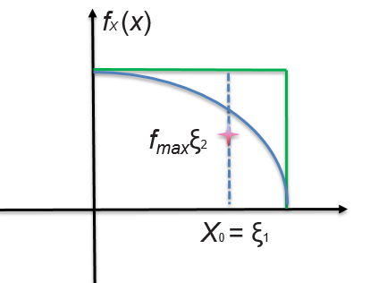
Figure 1: A geometric view of the rejection method.

Here, the rejection method can be viewed as to choose uniformly the points enclosed by the curve $f(x)$ inside the smallest rectangle that contains the curve. The ordinate of such a point is $x_{0}=\xi_{1}$; the abscissa is $f_{max}\xi_{2}$. Points lying above the curve are rejected; points below are accepted. Their ordinates $x=x_{0}$ have the distribution $f(x)$. For example, consider the following probability distribution function:

$$f(x)=\frac{1}{1+2x^{2}},0<x<1$$ (31)

This can be sampled using the following steps:

1. $x_{0}=\xi_{1}$

2. if $\xi_{2}>\frac{1}{1+2x_{0}^{2}}$, repeat from 1; else $x=x_{0}$.

where $\xi_{1}$ and $\xi_{2}$ are two uniformly sampled random numbers between zero and one. Another example of using the rejection method is to sample a uniform density distribution within a unit circle. This can be done as follows:

1. $x_{0}=\xi_{1}$, and $y_{0}=\xi_{2}$

2. if $x_{0}^{2}+y_{0}^{2}>1$, repeat from 1; else $x=x_{0}$ and $y=y_{0}$.

The above rejection method requires the information of the maximum value of the sampled probability distribution function within the domain in order to calculate the normalized function value $\frac{f(x_{0})}{f_{max}}$. The efficiency of the rejection method depends on the ratio of $f(x_{0})/f_{max}$. In many applications, this ratio can be small, e.g. the tail of a Gaussian distribution. This suggests that many trial solutions will be rejected before attaining a sampled point. For some complex probability distribution function, the maximum of the function is not easily accessible. However, if one can find an easily sampled function $g(x)$ so that $Mg(x)\geq f(x)$ with constant $M>1$ for all $x$, a general rejection method can be written as [8]:

• generate a random number $x_{0}$ between $x_{min}$ and $x_{max}$ from the sampling of $g(x)$.

• generate a uniform random number $\xi_{1}$ between $0$ and $1$.

• if $\xi_{1}\leq f(x_{0})/(Mg(x_{0}))$: accept $x_{0}$.

• otherwise; reject $x_{0}$.

If one choose the $g(x)=f_{max}/M$, a uniform distribution, the above general rejection method is reduced to the preceding rejection method. It is clear that the efficiency of the above rejection method depends on the ratio of $f(x)/Mg(x)$.

0.3.4 Markov chain Monte Carlo

The efficiency of the rejection method can be improved by another general sampling method, Metropolis method or in general also called Markov chain Monte Carlo (MCMC) method. The Markov chain Monte Carlo method is a general method to sample any probability distribution function regardless of its analytic complexity in any number of dimensions. It does not need to know either the maximum or the upper bound of the sampled probability distribution function. Moreover, it does not reject all samplings with $f(x_{0})/f_{max}<\xi_{2}$ in the rejection method but with a probability of acceptance depending on the local function value. This makes it more efficient than the rejection method. Some disadvantages of the MCMC are that the sampling is correct only asymptotically and that successive samplings are correlated. To avoid these disadvantages, some initial samplings are thrown away (called burn-in phase) and the used samplings are separated by a number of steps.

A sequence of random variables $x_{i},i=1,2,\ldots$ forms a Markov chain if:

$$P(x_{i+1}=x|x_{1},\cdots,x_{i})=P(x_{i+1}=x|x_{i})$$ (32)

That is, the probability distribution of $x_{i+1}$ depends only on the previous step $x_{i}$, and is independent of other steps ($x_{i-1},\ldots,x_{1}$) before. A Markov chain is said to be ergodic if it satisfies the following conditions [9, 10, 11]:

• Irreducible: Any state can be reached from any other state with nonzero probability.

• Positive recurrent: For any state A, the expected number of steps required for the chain to return to A is finite.

• Aperiodic: For any state A, the number of steps required to return to A must not always be a multiple of some integer value.

In other words, it means that all possible states of the system will be reached within some finite number of steps. If there exists a distribution function $f(x)$ such that $f(x_{i+1})P(x_{i+1}|x_{i})=f(x_{i})P(x_{i}|x_{i+1})$ for all $i$, the Markov chain is reversible and the $f(x)$ is then the equilibrium distribution of the Markov chain. Provided that a Markov chain is ergodic it will converge to an equilibrium stationary distribution. This stationary distribution is determined entirely by the transition probabilities of the chain. The initial value of the chain is irrelevant in the long run. This suggests that the sampling based on the Markov chain would sample the probability distribution $f(x)$ asymptotically. The Metropolis Markov chain Monte-Carlo algorithm to sample an arbitrary distribution can be summarized as:

1. choose a proposal transition probability distribution $p(x)$ and an initial random sampled value $x_{1}$.

2. calculate a new trial value ${\bar{x}}=x_{i}+\tau$ using an update step $\tau$ sampled from $p(x)$.

3. if $f(\bar{x})>f(x_{i})$ accept $x_{i+1}=\bar{x}$, otherwise accept $x_{i+1}=\bar{x}$ with a probability $f({\bar{x}})/f(x_{i})$.

4. continue step 2 until one has enough number of sampled values.

5. discard some early values during the burn-in phase.

Typically, the proposal distribution function can be assumed as a Gaussian function $p(x)=\mathcal{N}(0,\sigma)$ or a uniform distribution $p(x)=\mathcal{U}(-v,v)$ [12].

The above symmetric proposal transition distribution might not be optimal. In order to speed up convergence, a correction factor, the Hastings ratio, is applied to correct for the bias. The probability to accept the new trial sampling value is modified from the original $min(1,f(\bar{x}/f(x_{i}))$ to include the Hastings ratio $min(1,f(\bar{x})p({\bar{x}};x_{i})/(f(x_{i})p(x_{i};\bar{x}))$. If $p({\bar{x}};x_{i})=p(x_{i};{\bar{x}})$, this is the Metropolis algorithm.

In practical application, the width of the proposal distribution (e.g. for a Gaussian update or for a uniform update) should be tuned during the burn-in phase to set the rejection fraction in the right range. The conventional acceptance probability is typically between $30\%$ and $70\%$. One can use the autocorrelation function to check if the initial value has become irrelevant or not. In order to break the dependence between successive draws in the Markov chain, one might keep only every $n^{th}$ draw of the chain. To check whether a Markov chain reaches an equilibrium distribution or not, one can use multiple chains. When the variance between multiple chains is much less than the variance within the chains, the chain reaches the equilibrium. One can also monitor the behaviour of an expectation value that evolves with the length of the Markov chain random walk. Figure 2 shows the evolution of the expectation value calculated from $100$ samplings as a function of the random walk steps.

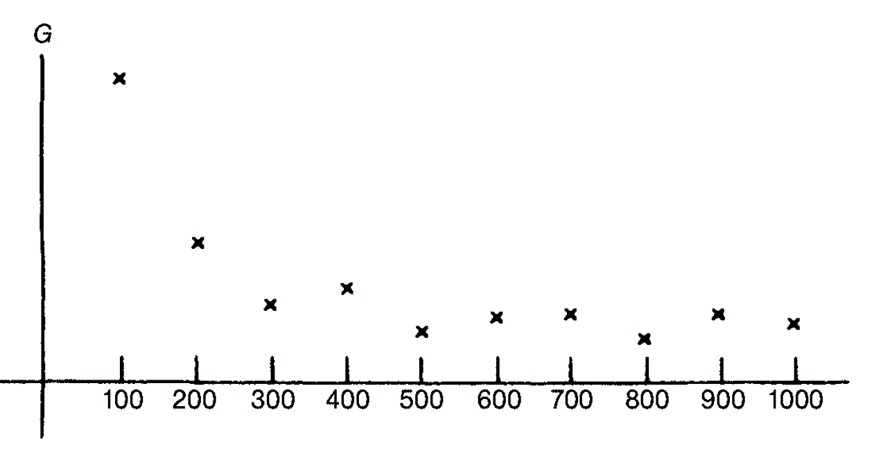
Figure 2: Behaviour of <G> with length of the $M(RT)^{2}$ random walk [2].

It is seen that after $400$ random walks, the expectation value starts to fluctuate. This suggests that the chain might have reached an equilibrium state.

0.4 Numerical integration using the Monte Carlo method

One of the most important applications of the Monte Carlo method is to calculate the integral. Given the following integral:

$$G=\int g(x)f(x)dx,\ \ f(x)\geq 0\ and\ \int f(x)=1$$ (33)

one can sample the probability distribution function $f(x)$ and form the arithmetic mean as:

$$G_{N}=\frac{1}{N}\sum_{i}g(x_{i})$$ (34)

where $N$ is the number of sampling points. The original integration can be written as:

$$G=G_{N}+error$$ (35)

with

$$|error|\simeq\frac{\sigma}{\sqrt{N}}$$ (36)

where

$$\sigma^{2}=\int g^{2}(x)f(x)dx-G^{2}$$ (37)

denotes the variance of the function $g(x)$. The error will decrease as $1/\sqrt{N}$ independent of dimensionality of the integral. This is the key advantage of the Monte Carlo method over the direct numerical quadrature whose computational cost scales exponentially with the number of dimensions. In order to reduce the error in the calculation of the integral using the Monte Carlo method, for a given number of samplings, one needs to reduce the variance of the integrand or to improve on the scaling with respect to the number of samplings. In the following, we will introduce several variance reduction methods and a quasi-Monte Carlo method to reduce the numerical error in the evaluation of the integral using the Monte Carlo method.

0.4.1 Importance sampling for variance reduction

Given the initial integral Eq. 33, we can rewrite the integral as:

$$G=\int\frac{g(x)f(x)}{\bar{f}(x)}{\bar{f}}(x)dx$$ (38)

where $\bar{f}(x)$ is a new probability density function. Using the sampling from this new probability distribution function, the numerical integral can be written as:

$$G_{N}=\frac{1}{N}\sum_{i}\frac{g(x_{i})f(x_{i})}{\bar{f}(x_{i})}$$ (39)

The variance of the new integrand becomes:

$$\bar{\sigma}^{2}=\int\frac{g^{2}(x)f^{2}(x)}{\bar{f}(x)}dx-G^{2}$$ (40)

Ideally, the optimal $\bar{f}(x)$ should be chosen as $g(x)f(x)/G$ [2]. In practice, a similar function to the integrand $g(x)f(x)$ can be used as $\bar{f}(x)$ to reduce the variance. For example, consider the following integral:

$$G=\int_{0}^{1}\cos(x)dx$$ (41)

A straightforward Monte Carlo algorithm would be to sample a uniform probability density function $f(x)$ between [0, 1], and then to calculate the mean quantity $<\cos(x)>$. The variance of this direct Monte Carlo calculation is $0.01925$. If we approximate the original function as:

$$\cos(x)\approx 1-\frac{x^{2}}{2}$$ (42)

and choose ${\bar{f}}(x)=\frac{6}{5}(1-x^{2}/2)$ as the importance sampling function, the new function will be:

$${\bar{g}}(x)=\frac{\cos(x)}{{\bar{f}}(x)}=\frac{10}{6}\frac{\cos(x)}{2-x^{2}}$$ (43)

The variance of the new function is $0.0001949$. This is about two orders of magnitude reduction of the variance in comparison to the direct Monte-Carlo method.

0.4.2 Correlation methods for variance reduction

Besides the importance sampling method to reduce the variance, another way to reduce the variance is to make use some function whose integral can be calculated analytically. Using the analytically integrable function $h(x)$, the original integral Eq. 33 can be rewritten as:

$$G=\int(g(x)-h(x))f(x)dx+\int h(x)f(x)dx$$ (44)

Here, we assume that the second integral can be obtained analytically. Using the Monte Carlo method to sample the probability distribution $f(x)$, the above integral can be approximated as:

$$G\simeq\frac{1}{N}\sum_{i}(g(x_{i})-h(x_{i}))+\int h(x)f(x)dx$$ (45)

If the variance of $g(x)-h(x)$, is much less than the variance of the original function $g(x)$, especially, if $|g(x)-h(x)|$ is approximately constant for different values of $h(x)$, then the above correlated sampling would be an efficient variance reduction method. For example, consider the following integral:

$$G=\int_{0}^{1}\sin(x)dx$$ (46)

The variance of $G$ using the direct Monte Carlo method following a uniform probability distribution function is $0.0614$. If we choose $h(x)=x$, the variance of $\sin(x)-x$ following the same uniform probability distribution is $0.00205$, which is more than an order of magnitude less than the variance of the original function.

0.4.3 Method of antithetic variates

This method exploits the fact that the decrease in variance occurs when random variables are negatively correlated. Consider the following integral:

$$G=\int_{0}^{1}g(x)dx$$ (47)

This integral can be rewritten as:

$$G=\int_{0}^{1}\frac{1}{2}[g(x)+g(1-x)]dx$$ (48)

and

$$G_{N}=\frac{1}{N}\sum_{i}[g(x_{i})+g(1-x_{i})]$$ (49)

If $g(x)$ is a linear function of $x$, the variance of the above integration will be zero. For nearly linear functions, this method will substantially reduce the variance. For example, consider the following integral:

$$G=\int_{0}^{1}e^{-x}dx$$ (50)

The variance using the direct Monte Carlo method (assuming a uniform density function $f(x)$) is $0.019$. Using the above method, the variance is reduced to $0.00053$, another order of magnitude reduction of the variance.

0.4.4 Quasi-Monte Carlo non-random sampling

As seen from the Eq. 36, in order to reduce the error in numerical integration using the Monte Carlo method, besides reducing the variance of integral using the preceding methods, another way is to improve on the scaling with respect to the number of samplings. A quasi-Monte Carlo sampling is a method that uses a non-random sequence to sample the uniform distribution between zero and one. Sampling an arbitrary probability distribution can then be attained through the transformation of the sampling of the uniform distribution. A non-random sequence that has low discrepancy (a measure of deviation from uniformity) can be used to simulate the uniform distribution. A popular non-random Halton/Hammersley sequence in multiple dimensions is defined as follows [13]:

$$X = {(j-1/2)/N,\Phi_{2}(j),\Phi_{3}(j),\ldots,\Phi_{r}(j)},\ \ j=1,\ldots,N$$ (51)

$$j = a_{0}+a_{1}r^{1}+\ldots$$ (52)

$$\Phi_{r}(j) = a_{0}r^{-1}+a_{1}r^{-2}+\ldots$$ (53)

where $\Phi_{r}(j)$ is the radical inversion function in the base of a prime number $r$. For example, using base number $3$, and $j=1,2,3,4$ one obtains the sequence: $\Phi_{3}(1)=1/3$, $\Phi_{3}(2)=2/3$, $\Phi_{3}(3)=1/9$, $\Phi_{3}(4)=4/9$. Figure 3 shows $1000$ samplings of a two-dimensional uniform distribution from using the random sampling and from the non-random Halton sequence. It is seen that the non-random sampling populates the two-dimensional square more uniformly than the random sampling. Fluctuation of this type of sequence scales as $1/N$ whereas a random Monte Carlo sampling scales as $1/\sqrt{N}$. The error in some cases of numerical integration using the non-random sampling can reach $1/N$ [6].

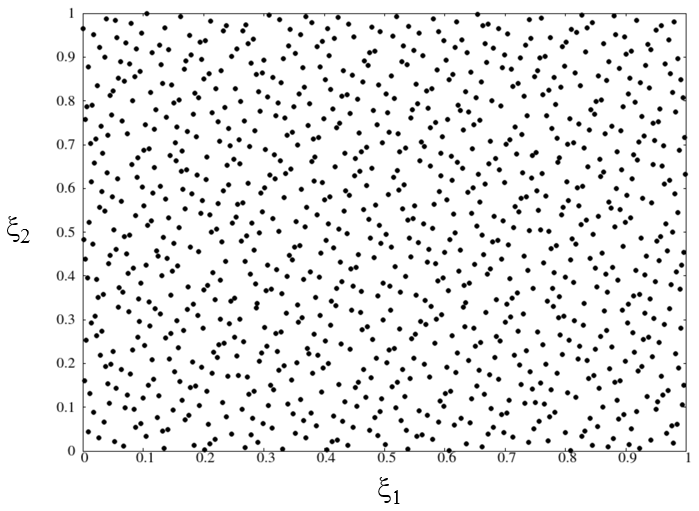
Figure 3: Two dimensional uniform sampling from the Fortran pseudo-random number generator (left) and the Halton sequence (right).

References

- [1] J. H. Halton, SIAM Review, Vol. 12, No. 1 (1970).
- [2] M. H. Kalos and P. A. Whitlock, Monte Carlo Methods, 2nd ed. WILEY-VCH Verlag GmbH & Co., Weinheim, 2008.
- [3] https://en.wikipedia.org/wiki/Monte_Carlo_method.
- [4] M. E. J. Newman, G. T. Barkema, Monte Carlo Methods in Statistical Physics, Oxford University Press, Oxford, 2001.
- [5] P. Glasserman, Monte Carlo Methods in Financial Engineering, (Springer Science+Business Media, New York, 2003).
- [6] W. H. Press, S. A. Teukolsky, W. T. Vetterling, B. P. Flannery, Numerical Recipes in FORTRAN, 2nd ed. Cambridge University Press, Cambridge, 1992.
- [7] G. E. P. Box and M. E. Muller, The Annals of Mathematical Statistics. 29 (2): 610-611, 1958.
- [8] https://en.wikipedia.org/wiki/Rejection_sampling.
- [9] https://en.wikipedia.org/wiki/Markov_chain.
- [10] P. Lam, http://patricklam.org/teaching/mcmc_print.pdf.
-
[11]
P. Breheny,
https://web.as.uky.edu/statistics/users/pbreheny/701/S13/notes/2-28.pdf. - [12] S. Paltani, https://www.unige.ch/sciences/astro/files/2713/8971/4086/3_Paltani_MonteCarlo.pdf.
- [13] S. M. Lavalle, Planning Algorithms, Cambridge University Press, New York, 2006.