Competitive Policy Optimization

Abstract

A core challenge in policy optimization in competitive Markov decision processes is the design of efficient optimization methods with desirable convergence and stability properties. To tackle this, we propose competitive policy optimization (CoPO), a novel policy gradient approach that exploits the game-theoretic nature of competitive games to derive policy updates. Motivated by the competitive gradient optimization method, we derive a bilinear approximation of the game objective. In contrast, off-the-shelf policy gradient methods utilize only linear approximations, and hence do not capture interactions among the players. We instantiate CoPO in two ways: $(i)$ competitive policy gradient, and $(ii)$ trust-region competitive policy optimization. We theoretically study these methods, and empirically investigate their behavior on a set of comprehensive, yet challenging, competitive games. We observe that they provide stable optimization, convergence to sophisticated strategies, and higher scores when played against baseline policy gradient methods.

1 Introduction

Reinforcement learning (RL) in competitive Markov decision process CoMDP (Filar and Vrieze, 2012) is the study of competitive players, sequentially making decisions in an environment (Puterman, 2014; Sutton and Barto, 2018). In CoMDPs, the competing agents (players) interact with each other within the environment, and through their interactions, learn how to develop their behavior and improve their notion of reward. In this paper, we considered the rich and fundamental class of zero-sum two-player games. Applications of such games abound from hypothesis testing (Wald, 1945), generative adversarial networks (Goodfellow et al., 2014), Lagrangian optimization (Dantzig, 1998), online learning (Cesa-Bianchi and Lugosi, 2006), algorithmic game theory (Roughgarden, 2010), robust control (Zhou et al., 1996), to board games (Tesauro, 1995; Silver et al., 2016).

In these applications, two players compete against each other, potentially in unknown environments. One goal is to learn policies/strategies for agents by making them play against each other. Due to the competitive nature of games, RL methods that do not account for the interactions are often susceptible to poor performance and divergence even in simple scenarios. One of the core challenges in such settings is to design optimization paradigms with desirable convergence and stability properties.

Policy gradient (PG) is a prominent RL approach that directly optimizes for policies, and enjoys simplicity in implementation and deployment (Robbins and Monro, 1951; Aleksandrov et al., 1968; Sutton et al., 2000). PG updates are derived by optimizing the first order (linear) approximation of the objective function while regularizing the parameter deviations. In two-player zero-sum CoMDPs, policy updates of the maximizing (minimizing) agent are derived through maximizing (resp. minimizing) the linear approximation of the game objective with an additive (subtractive) regularization, resulting in the gradient descent ascent (GDA) PG algorithm. This approximation is linear in agents’ parameters and does not take their interaction into account. Therefore, GDA directly optimizes the policy of each agent by assuming the policy/strategy of the opponent is not updated, which can be a poor approach for competitive optimization.

We propose a new paradigm known as competitive policy optimization (CoPO), which exploits the game-theoretic and competitive nature of CoMDPs, and, instead, inspired by competitive gradient descent (Schäfer and Anandkumar, 2019), deploys a bilinear approximation of the game objective. The bilinear approximation is separately linear in each agent’s parameters and is built on agents’ interactions to derive the policy updates. To compute the policy updates, CoPO computes the Nash equilibrium of the bilinear approximation of the game objective with a (e.g., $\ell_{2}$) regularization of the parameter deviations. In CoPO, each agent derives its update with the full consideration of what the other agent’s current move and moves in the future time steps might be. Importantly, each agent considers how the environment, as the results of the agents’ current and future moves temporally, evolves in favor of each agent. Therefore, each agent hypothesizes about what the other agent’s and the environment’s responses would be, consequently resulting in the common recursive reasoning in game theory, especially temporal recursion in CoMDPs. We further show that CoPO is a generic approach that does not rely on the structure of the problem, at the cost of high sample complexity.

We instantiate CoPO in two ways to arrive at practical algorithms. We propose competitive policy gradient (CoPG), a novel PG algorithm that exploit value functions and structure of CoMDPs to efficiently obtain policy updates. We also propose trust region competitive policy optimization (TRCoPO), a novel trust region based PG method (Kakade and Langford, 2002; Schulman et al., 2015). TRCoPO optimizes a surrogate game objective in a trust region. TRCoPO updates agents’ parameters simultaneously by deriving the Nash equilibrium of bilinear (in contrast to linear approximation in off-the-shelf trust region methods) approximation to the surrogate objective within a defined trust region in the parameter space.

We empirically study the performance of CoPG and TRCoPO on six representative games, ranging from single-state to general sequential games, and tabular to infinite/continuous states/action games. We observe that CoPG and TRCoPO not only provide more stable and faster optimization, but also converge to more sophisticated, opponent aware, and competitive strategies compared with their conventional counterparts, GDA and TRGDA. When trained agents play against each other, we observe the superiority of CoPG and TRCoPO agents, e.g., in the Markov soccer game, CoPG agent beats GDA in 74%, and TRCoPO agent beats TRGDA in 85% of the matches. We observe a similar trend with other methods, such as multi-agent deep deterministic PG (MADDPG) (Lowe et al., 2017).

A related approach that uses a second-level reasoning (as opposed to CoPO with infinite-level reasoning) is LOLA (Foerster et al., 2017a), which shows positive results on three games, matching pennies, prisoners’ dilemma and a coin game. We compare LOLA against CoPG and TRCoPO and observe a similar trend in the superiority of CoPO based methods. We conclude the paper by arguing the generality of CoPO paradigm, and how it can be used to generalize single-agent PG methods to CoMDPs.

2 Preliminaries

A two player CoMDP is a tuple of $\langle\mathcal{S},\mathcal{A}^{1},\mathcal{A}^{2},\mathcal{R},\mathcal{T},\mathcal{P},\gamma\rangle$, where $\mathcal{S}$ is the state space, $s\in\mathcal{S}$ is a state, for player $i\in\{1,2\}$, $\mathcal{A}^{i}$ is the player $i$’s action space with $a^{i}\in\mathcal{A}^{i}$. $\mathcal{R}$ is the reward kernel with probability distribution $R(\cdot|s,a^{1},a^{2})$ and mean function $r(s,a^{1},a^{2})$ on $\mathbb{R}$. For a probability measure $\mathcal{P}$, $p$ denotes the probability distribution of initial state, and for the transition kernel $\mathcal{T}$, $T(s^{\prime}|s,a^{1},a^{2})$ is the distribution of successive state $s^{\prime}$ after taking actions $a^{1},a^{2}$ simultaneously at state $s$, with discount factor $\gamma\in[0,1]$. We consider episodic environments with reachable absorbing state $s_{T}$ almost surely in finite time. An episode starts at $s_{0}\sim p$, and at each time step $k\geq 0$ at state $s_{k}$, each player $i$ draws its action $a_{k}^{i}$ according to policy $\pi(a_{k}^{i}|s_{k};\theta^{i})$ parameterized by $\theta^{i}\in\Theta^{i}$, where $\Theta^{i}\subset\mathbb{R}^{l}$ is a compact metric space. Players $1,2$ receive $(r_{k},-r_{k})$ with $r_{k}\sim R(s_{k},a^{1}_{k},a^{2}_{k})$, and the environment evolves to a new state $s_{k+1}$. A realization of this stochastic process is a trajectory $\tau=\big{(}(s_{k},a^{1}_{k},a^{2}_{k},r_{k})_{k=0}^{|\tau|-1},s_{|\tau|}\big{)}$, an ordered sequence with random length $|\tau|$, where $|\tau|$ is determined by episode termination time and state $s_{|\tau|}=s_{T}$. Let $f(\tau;\theta^{1},\theta^{2})$ denote the probability distribution of the trajectory $\tau$ following players’ policies $\pi(\theta^{i})$,

$$f(\tau;\theta^{1},\theta^{2})=p(s_{0})\prod_{k=0}^{|\tau|-1}\pi(a^{1}_{k}|s_{k};\theta^{1})\pi(a^{2}_{k}|s_{k};\theta^{2})R(r_{k}|s_{k},a^{1}_{k},a^{2}_{k})T(s_{k+1}|s_{k},a^{1}_{k},a^{2}_{k}).\vspace{-3.00mm}$$ (1)

For $R(\tau)=\sum_{k=0}^{|\tau|}\gamma^{k}r(s_{k},a^{1}_{k},a^{2}_{k})$, the $Q$-function, $V$-functions, and game objective are defined,

$$\quad\quad\quad\quad Q(s_{k},a^{1}_{k},a^{2}_{k};\theta^{1},\theta^{2})=\mathbb{E}_{\tau\sim f(\cdot;\theta^{1},\theta^{2})}\Big{[}\sum\nolimits_{j=k}^{|\tau|-1}\!\gamma^{j-k}r(s_{j},a^{1}_{j},a^{2}_{j})|s_{k},a^{1}_{k},a^{2}_{k}\Big{]},$$ (2)

$$\!\!V(s_{k};\theta^{1},\theta^{2})=\mathbb{E}_{\tau\sim f(\cdot;\theta^{1},\theta^{2})}\Big{[}\sum\nolimits_{j=k}^{|\tau|-1}\!\gamma^{j-k}r(s_{j},a^{1}_{j},a^{2}_{j})|s_{k}\,\Big{]},~{}\eta(\theta^{1},\theta^{2})=\!\!\int_{\tau}\!f(\tau;\theta^{1},\theta^{2})R(\tau)d\tau\vspace{-3.00mm}$$

We assume $V$, $Q$, and $\eta$ are differentiable and bounded in $(\Theta^{1},\Theta^{2})$ and for $f$ on $(\Theta^{1}$ $\Theta^{2})$, $D_{\theta^{i}}f=\frac{\partial}{\partial{\theta^{\prime}}^{i}}f({\theta^{\prime}}^{1}\!\!,\!{\theta^{\prime}}^{2})\big{|}_{({\theta^{\prime}}^{1},{\theta^{\prime}}^{2})=({\theta}^{1},{\theta}^{2})}$, and $D_{\theta^{i}\theta^{j}}f=\frac{\partial}{\partial{\theta^{\prime}}^{i}}\big{(}\frac{\partial}{\partial{\theta^{\prime}}^{j}}f({\theta^{\prime}}^{1}\!\!,\!{\theta^{\prime}}^{2})\big{)}\big{|}_{({\theta^{\prime}}^{1},{\theta^{\prime}}^{2})=({\theta}^{1}\!,{\theta}^{2})}$, for $i,j\in\{1,2\}$.

3 Competitive Policy Optimization

Player 1 aims to maximize the game objective $\eta$ Eq. (2), while player 2 aims to minimize it, i.e., simultaneously solving for $\max_{\theta^{1}}\eta(\theta^{1},\theta^{2})$ and $\min_{\theta^{2}}\eta(\theta^{1},\theta^{2})$ respectively with,

$$\theta^{1*}\in\operatorname*{arg\,max}\nolimits_{\theta^{1}\in\Theta^{1}}\eta(\theta^{1},\theta^{2}),~{}\text{and}~{}~{}\theta^{2*}\in\operatorname*{arg\,min}\nolimits_{\theta^{2}\in\Theta^{2}}\eta(\theta^{1},\theta^{2}).$$ (3)

As discussed in the introduction, a straightforward generalization of PG methods to CoMDP, results in GDA (Alg.1). Given players’ parameters $(\theta^{1},\theta^{2})$, GDA prescribes to optimize a linear approximation of the game objective in the presence of a regularization for the policy updates,

$$\!\!\!\!\theta^{1}\!\leftarrow\!\theta^{1}\!+\!\!\!\operatorname*{arg\,max}_{{\Delta\theta}:{\Delta\theta}+\theta\in\Theta^{1}}\!\!\!{\Delta\theta}^{\top}\!D_{{\theta}^{1}}\eta-\frac{1}{2\alpha}||{\Delta\theta}||^{2}\!,~{}\text{and}\ \theta^{2}\leftarrow\theta^{2}\!\!+\!\!\!\operatorname*{arg\,min}_{{\Delta\theta}:{\Delta\theta}+\theta\in\Theta^{2}}\!\!\!{\Delta\theta}^{\top}\!D_{{\theta}^{2}}\eta+\frac{1}{2\alpha}||{\Delta\theta}||^{2}\!,\!\!$$ (4)

where $\alpha$ represent the step size. The parameter updates in Eq. 4 result in greedy updates along the directions of maximum change, assuming the other player stays constant. These updates are myopic, and ignore the agents’ interactions. In other words, player 1 does not take player’s 2 potential move into consideration and vice versa. While GDA might be an approach of interest in decentralized CoMDP, it mainly falls short in the problem of competitive and centralized optimization in unknown CoMDPs, i.e., the focus of this work. In fact, this behaviour is far from optimal and is shown to diverge in many simple cases e.g. plain bilinear or linear quadratic games  (Schäfer and Anandkumar, 2019; Mazumdar et al., 2019).

We propose competitive policy optimization CoPO, a policy gradient approach for optimization in unknown CoMDPs. In contrast to standard PG methods, such as GDA, CoPO considers a bilinear approximation of the game objective, and takes the interaction between players into account. CoPO incorporates the game theoretic nature of the CoMDP optimization and derives parameter updates through finding the Nash equilibrium of the bilinear approximation of the game objective,

$$\theta^{1}\leftarrow\theta^{1}+\operatorname*{arg\,max}\nolimits_{{\Delta\theta^{1}}:{\Delta\theta^{1}}+\theta^{1}\in\Theta^{1}}{\Delta\theta^{1}}^{\top}D_{{\theta}^{1}}\eta+{\Delta\theta^{1}}^{\top}D_{\theta^{1}\theta^{2}}\eta{\Delta\theta^{2}}-\frac{1}{2\alpha}||{\Delta\theta}^{1}||^{2},$$

$$\theta^{2}\leftarrow\theta^{2}+\operatorname*{arg\,min}\nolimits_{{\Delta\theta^{2}}:{\Delta\theta^{2}}+\theta^{2}\in\Theta^{2}}{\Delta\theta^{2}}^{\top}D_{{\theta}^{2}}\eta+{\Delta\theta^{2}}^{\top}D_{\theta^{2}\theta^{1}}\eta{\Delta\theta^{1}}+\frac{1}{2\alpha}||{\Delta\theta}^{2}||^{2},$$ (5)

which has an extra term, the interaction term, in contrast to Eq. 4, and has the following closed-form solution,

$$\theta^{1} \leftarrow\theta^{1}+\alpha\bigl{(}I+\alpha^{2}D_{\theta^{1}\theta^{2}}\eta D_{\theta^{2}\theta^{1}}\eta\bigr{)}^{-1}\bigl{(}D_{\theta^{1}}\eta-\alpha D_{\theta^{1}\theta^{2}}\eta D_{\theta^{2}}\eta\bigr{)},$$

$$\theta^{2} \leftarrow\theta^{2}-\alpha\bigl{(}I+\alpha^{2}D_{\theta^{2}\theta^{1}}\eta D_{\theta^{1}\theta^{2}}\eta\bigr{)}^{-1}\bigl{(}D_{\theta^{2}}\eta+\alpha D_{\theta^{2}\theta^{1}}\eta D_{\theta^{1}}\eta\bigr{)},$$ (6)

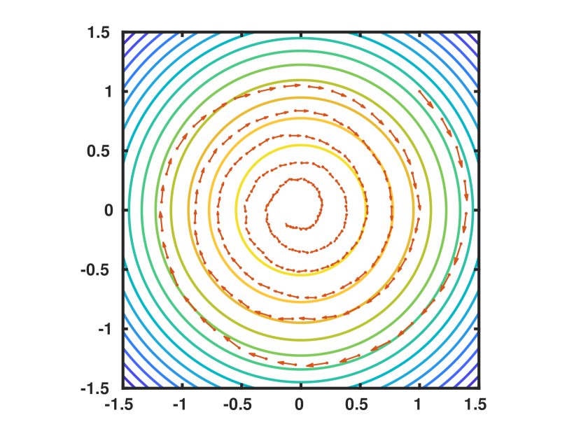
(a) CoPO

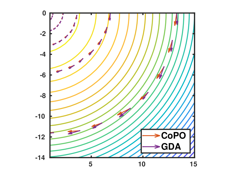
(b) CoPO vs GDA ​​​​​​​​​​​​​​​​​​​​​​​​​​​​​​​​​​​​

Figure 1: Bilinear games: (a) CoPO updates towards Nash equilibrium. (b) GDA updates point outward, leading to cycling/divergence.

where $I$ is an identity matrix of appropriate size. Note that, the bilinear approximation in Eq. 3 is still linear in each player’s action/parameters. Including any other terms, e.g., block diagonal Hessian terms from the Taylor expansion of the game objective, results in nonlinear terms in at least one player’s parameters. As such, CoPO can be viewed as a natural linear generalization of PG. It is known that GDA-style co-learning approaches can often diverge or cycle indefinitely and never converge (Mertikopoulos et al., 2018a). Fig. 1 shows that for a bilinear game, the gradient flow of GDA cycles or has gradient flow outward, while the CoPG flow, considering players’ future moves, has gradient flow toward the Nash equilibrium and converges. In Apx.B, we deploy the Neumann series expansion of the inverses in Eq.3, and show that CoPO recovers the infinite recursion reasoning between players and the environment, while GDA correspond to the first term, and LOLA corresponds to the first two terms in the series. Next, we compute terms in Eq. 3 using the score function $g(\tau,\theta^{i}):=D_{\theta^{i}}(\log\prod_{k=0}^{|\tau|-1}\pi(a_{k}|s_{k};\theta^{i}))$,

Proposition 1.

Given a CoMDP, players $i,j\in\!\{1,2\}$, $i\neq j$ and the policy parameters $\theta^{i},\theta^{j}$,

$$D_{{\theta}^{i}}\eta=\int_{\tau}f(\tau;\theta^{1},\theta^{2})g(\tau,\theta^{i})R(\tau)d\tau,\textit{and}~{}D_{\theta^{i}\theta^{j}}\eta\!=\int_{\tau}f(\tau;\theta^{1},\theta^{2})g(\tau,\theta^{i})g(\tau,\theta^{j})^{\top}R(\tau)d\tau.$$

Proof in Apx. C.1. In practice, we use conjugate gradient and Hessian vector product to efficiently compute the updates in Eq.3, as explained in later sections. A closer look at CoPO shows that this paradigm does not require the knowledge of the environment if sampled trajectories are available. It neither requires full observability of the sates, nor any structural assumption on CoMDP, but the Monte Carlo estimation suffer from high variance. In the following, we explicitly take the CoMDP structure into account to develop efficient algorithms.

3.1 Competitive Policy Gradient

We propose competitive policy gradient (CoPG), an efficient algorithm that exploits the structure of CoMDPs to compute the parameter updates. The following is the CoMDP generalizing of the single agent PG theorem  (Sutton et al., 2000). For $\tau_{l:l^{\prime}}=(s_{k},a^{1}_{k},a^{2}_{k},r_{k})_{k=l}^{l^{\prime}}$, the events from time step $l$ to $l^{\prime}$, we have:

Theorem 1.

Given a CoMDP, players $i,j\in\!\{1,2\}$, $i\neq j$, and the policy parameters $\theta^{i},\theta^{j}$,

$$\!\!\!\!\!\!\!\!\!\!\!\!\!\!\!\!\!\!\!\!\!\!\!\!\!\!\!D_{\theta^{i}}\eta =\int_{\tau}\!\!\sum_{k=0}^{|\tau|-1}\gamma^{k}f(\tau_{0:k};\theta^{1},\theta^{2})D_{\theta^{i}}(\log\pi(a_{k}^{i}|s_{k};\theta^{i}))Q(s_{k},a_{k}^{1},a_{k}^{2};\theta^{1}\!\!,\theta^{2})d\tau,\!\!\!\!\!$$ (7)

$$\!\!D_{\theta^{i}\theta^{j}}\eta =\!(\widehat{1})\!\!:\!\!\!\int_{\tau}\!\!\!\sum_{k=0}^{|\tau|-1}\!\!\!\gamma^{k}\!f(\!\tau_{0:k};\theta^{1}\!\!,\theta^{2})D_{\theta^{i}}(\log\pi(\!a_{k}^{i}|s_{k};\theta^{i}))D_{\theta^{j}}(\log\pi(\!a_{k}^{j}|s_{k};\theta^{j}))^{\!\top}\!Q(\!s_{k},a_{k}^{1},a_{k}^{2};\theta^{1}\!\!,\theta^{2})d\tau$$

$$\!\!\!\!\!\!\!\!\!\!\!\!\!\!\!\!\!+\!(\widehat{2})\!:\!\!\!\int_{\tau}\!\!\sum_{k=1}^{|\tau|-1}\!\!\!\gamma^{k}\!f(\!\tau_{0:k};\theta^{1}\!,\!\theta^{2})D_{\theta^{i}}(\log\!\!\prod_{l=0}^{k-1}\!\!\pi(\!a_{l}^{i}|s_{l};\theta^{i}))D_{\theta^{j}}(\log\pi(\!a_{k}^{j}|s_{k};\theta^{j}))\!^{\top}\!Q(\!s_{k},a_{k}^{1},a_{k}^{2};\theta^{1}\!\!,\theta^{2})d\tau\$$

$$\!\!\!\!\!\!\!\!\!\!\!\!\!\!\!\!\!+\!(\widehat{3})\!\!:\!\!\!\int_{\tau}\!\!\sum_{k=1}^{|\tau|-1}\!\!\!\gamma^{k}\!f(\!\tau_{0:k};\theta^{1}\!\!,\!\theta^{2})D_{\theta^{i}}(\log\pi(\!a_{k}^{i}|s_{k};\theta^{i}))D_{\theta^{j}}(\log\!\!\prod_{l=0}^{k-1}\!\!\pi(\!a_{l}^{j}|s_{l};\theta^{j}))\!^{\top}\!Q(\!s_{k},a_{k}^{1},a_{k}^{2};\theta^{1}\!\!,\theta^{2})d\tau.\!\!\!\!\!\!\!\!\!\!$$ (8)

Proof in Apx. C.2. This theorem indicates that the terms in Eq. 3 can be computed using $Q$ function. In Eq. 8, ($\widehat{1}$) is the immediate interaction between players, ($\widehat{2}$) is the interaction of player $i$’s behavior up to time step $k$ with player $j$’s reaction at time step $k$, and the environment. ($\widehat{3}$) is the interaction of player $j$’s behavior upto time step $k$ with player $i$’s reaction at time step $k$, and the environment.

CoPG operates in epochs. At each epoch, CoPG deploys $\pi(\theta^{1})$, $\pi(\theta^{2})$ to collect trajectories, exploits them to estimate the $Q$, $D_{\theta^{i}}\eta$, and $D_{\theta^{i}\theta^{j}}\eta$. Then CoPG follows the parameter updates in Eq. 3 and updates $(\theta^{1}\!\!,\theta^{2})$, and this process goes on to the next epoch (Alg.2). Many variants of PG approach uses baselines, and replace $Q$ with, the advantage function $A(s,a^{1},a^{2};\theta^{1},\theta^{2})=Q(s,a^{1},a^{2};\theta^{1},\theta^{2})-V(s;\theta^{1},\theta^{2})$, Monte Carlo estimate of Q-V (Baird, 1993), empirical TD error or generalized advantage function (GAE) (Schulman et al., 2016). Our algorithm can be extended to this set up and in Apx. D we show how CoPG can be accompanied with all the mentioned variants.

3.2 Trust Region Competitive Policy Optimization

Trust region based policy optimization methods exploit the local Riemannian geometry of the parameter space to derive more efficient policy updates (Kakade and Langford, 2002; Kakade, 2002; Schulman et al., 2015). In this section, we propose trust region competitive policy optimization (TRCoPO), the CoPO generalization of TRPO (Schulman et al., 2015), that exploits the local geometry of the competitive objective to derive more efficient parameter updates.

Lemma 1.

Given the advantage function of policies $\pi(\theta^{1}),\pi(\theta^{2})$, $\forall({\theta^{\prime}}^{1},{\theta^{\prime}}^{2})\in\Theta^{1}\times\Theta^{2}$ we have,

$$\eta(\theta^{\prime 1},\theta^{\prime 2})=\eta(\theta^{1},\theta^{2})+\mathbb{E}_{\tau\sim f(\cdot;\theta^{\prime 1},\theta^{\prime 2})}\sum\nolimits_{k=0}^{|\tau|-1}\gamma^{k}A(s,a^{1},a^{2};\theta^{1},\theta^{2}).$$ (9)

Proof in Apx. F.1. Eq.9 indicates that, considering our current policies $(\pi(\theta^{1}),\pi(\theta^{1}))$, having access to their advantage function, and also samples from $f(\cdot;\theta^{\prime 1},\theta^{\prime 2})$ of any $({\theta^{\prime}}^{1},{\theta^{\prime}}^{2})$ (without rewards), we can directly compute $\eta(\theta^{\prime 1},\theta^{\prime 2})$ and optimize for $(\theta^{\prime 1},\theta^{\prime 2})$. However, in practice, we might not have access to $f(\cdot;\theta^{\prime 1},\theta^{\prime 2})$ for all $({\theta^{\prime}}^{1},{\theta^{\prime}}^{2})$ to accomplish the optimization task, therefore, direct use of Eq.9 is not favorable. Instead, we define a surrogate objective function, $L_{\theta^{1},\theta^{2}}(\theta^{\prime 1},\theta^{\prime 2})$,

$$L_{\theta^{1},\theta^{2}}(\theta^{\prime 1},\theta^{\prime 2})\!\!=\!\eta(\theta^{1},\theta^{2})\!+\!\mathbb{E}_{\tau\sim f(\cdot;\theta^{1},\theta^{2})}\!\!\!\sum_{k=0}^{|\tau|-1}\!\!\gamma^{k}\mathbb{E}_{\pi(a^{\prime 1}_{k}|s_{k};\theta^{\prime 1}),\pi(a^{\prime 2}_{k}|s_{k};\theta^{\prime 2})}A(s_{k},a^{\prime 1}_{k},a^{\prime 2}_{k};\theta^{1},\theta^{2}),\!\!$$ (10)

which can be computed using trajectories of our current polices $\pi(\theta^{1}),\pi(\theta^{2})$. $L_{\theta^{1},\theta^{2}}({\theta^{\prime}}^{1},{\theta^{\prime}}^{2})$ is an object of interest in PG (Kakade and Langford, 2002; Schulman et al., 2015) since mainly its gradient is equal to that of $\eta(\theta^{1},\theta^{2})$ at $(\theta^{1},\theta^{2})$, and as stated in the following theorem, it can carefully be used as a surrogate of the game value. For KL divergence $D_{KL}((\theta^{1},\theta^{2}),(\theta^{\prime 1},\theta^{\prime 2})):=\int_{\tau}f(\tau,\theta^{1},\theta^{2})\log\big{(}f(\tau,\theta^{1},\theta^{2})/f(\tau,\theta^{\prime 1},\theta^{\prime 2})\big{)}d\tau$, we have,

Theorem 2.

$L_{\theta^{1},\theta^{2}}({\theta^{\prime}}^{1},{\theta^{\prime}}^{2})$ approximate $\eta({\theta^{\prime}}^{1},{\theta^{\prime}}^{2})$ up to the following error upper bound

$$|\eta(\theta^{\prime 1},\theta^{\prime 2})-L_{\theta^{1}\theta^{2}}(\theta^{\prime 1},\theta^{\prime 2})|\leq\epsilon/\sqrt{2}\sqrt{D_{KL}((\theta^{\prime 1},\theta^{\prime 2}),(\theta^{1},\theta^{2}))},$$ (11)

with constant $\epsilon:=\max_{\tau}\sum_{k}^{|\tau|}\gamma^{k}\mathbb{E}_{\pi(a^{\prime 1}_{k}|s_{k};\theta^{\prime 1}),\pi(a^{\prime 2}_{k}|s_{k};\theta^{\prime 2})}A(s_{k},a^{\prime 1}_{k},a^{\prime 2}_{k};\theta^{1},\theta^{2})$.

Proof in Apx. F.2. This theorem states that we can use $L_{\theta^{1}\theta^{2}}(\theta^{\prime 1},\theta^{\prime 2})$ to optimize for $\eta(\theta^{\prime 1},\theta^{\prime 2})$ as long as we keep the $(\theta^{\prime 1},\theta^{\prime 2})$ in the vicinity of $\theta^{1},\theta^{2}$. Similar to single agent TRPO (Schulman et al., 2015), we optimize for $L_{\theta^{1}\theta^{2}}(\theta^{\prime 1},\theta^{\prime 2})$, while constraining the KL divergence, $D_{KL}((\theta^{1},\theta^{2}),(\theta^{\prime 1},\theta^{\prime 2}))\leq\delta^{\prime}$, i.e.,

$$\max\nolimits_{\theta^{\prime 1}\in\Theta^{1}}\min\nolimits_{\theta^{\prime 2}\Theta^{1}}L_{\theta^{1}\theta^{2}}(\theta^{\prime 1},\theta^{\prime 2}),~{}\text{subject to: }D_{KL}((\theta^{1},\theta^{2}),(\theta^{\prime 1},\theta^{\prime 2}))\leq\delta^{\prime}.$$ (12)

The GDA generalizing of TRPO uses a linear approximation of $L_{\theta^{1}\theta^{2}}(\theta^{\prime 1},\theta^{\prime 2})$ to approach this optimization, which again ignores the players’ interactions. In contrast, TRCoPO considers the game theoretic nature of this optimization, and uses a bilinear approximation. TRCoPO operates in epochs. At each epoch, TRCoPO deploys $(\pi(\theta^{1}),\pi(\theta^{2}))$ to collect trajectories, exploits them to estimate $A$ (or GAE), then updates parameters accordingly, Alg.4. (For more details, please refer to Apx. F.3.)

4 Experiments

We empirically study the performance of CoPG and TRCoPO and their counterparts GDA and TRGDA, on six games, ranging from single-state repeated games to general sequential games, and tabular games to infinite/continuous states/action games. They are 1) linear-quadratic(LQ) game, 2) bilinear game, 3) matching pennies (MP), 4) rock paper scissors (RPS), 5) Markov soccer, and 6) car racing. These games are representative enough that their study provides insightful conclusions, and challenging enough to highlight the core difficulties and interactions in competitive games.

We show that CoPG and TRCoPO converge to stable points, and learn opponent aware strategies, whereas GDA’s and TRGDA’s greedy approach shows poor performance and even diverge in bi-linear, MP, and RPS games. For the LQ game, when GDA does not diverge, it almost requires 1.5 times the amount of samples, and is $1.5$ times slower than CoPG. In highly strategic games, where players’ policies are tightly coupled, we show that CoPG and TRCoPO learn much better interactive strategies. In the soccer game, CoPG and TRCoPO players learn to defend, dodge and score goals, whereas GDA and TRGDA players learn how to score when they are initialized with the ball, and give way to the other player otherwise. In the car racing, while GDA and TRGDA show poor performance, CoPG and TRCoPO produce competing players, which learn to block and fake each other. Overall, we observe CoPG and TRCoPO considerably outperform their counterparts in terms of convergence, learned strategies, and gradient dynamics. Note that in self-play, one player plays against itself using one policy model (neural network) for both players, is a special case of CoPO and we provide its detailed study in Apx. E.

We implemented all algorithms in Pytorch  (Paszke et al., 2019), and made the code and the videos public. In our implementation, we deploy Pytorch’s autograd package and Hessian vector product to efficiently obtain gradients and Hessian vector products to compute the bilinear terms in the optimizer. Moreover, we use the conjugate gradient trick to efficiently computed the inverses-matrix vector product in Eq.3 which incurs a minimal computational overhead (see (Shewchuk, 1994) for more details). To improve computation times, we compute inverse-matrix vector product only for one player strategy, and use optimal counter strategy for other player $\Delta\theta^{2}$ which is computed without an inverse matrix vector product. Also, the last optimal strategy can be used to warm start the conjugate gradient method which improves convergence times. We provide efficient implementation for both CoPO- and GDA-based methods, where CoPO incurs 1.5 times extra computation per batch.

Zero-sum LQ game is a continuous state-action linear dynamical game between two players, where GDA, with considerably small learning rate, has favorable convergence guarantees (Zhang et al., 2019). This makes the LQ game an ideal platform to study the range of allowable step sizes and convergence rate of CoPG and GDA. We show that, with increasing learning rate, GDA generates erratic trajectories and policy updates, which cause instability (see “$\oslash$” in Tab. 2), whereas CoPG is robust towards this behavior. Fig. 2(a) shows that CoPG dynamics are not just faster at the same learning rate but more importantly, CoPG can potentially take even larger steps.

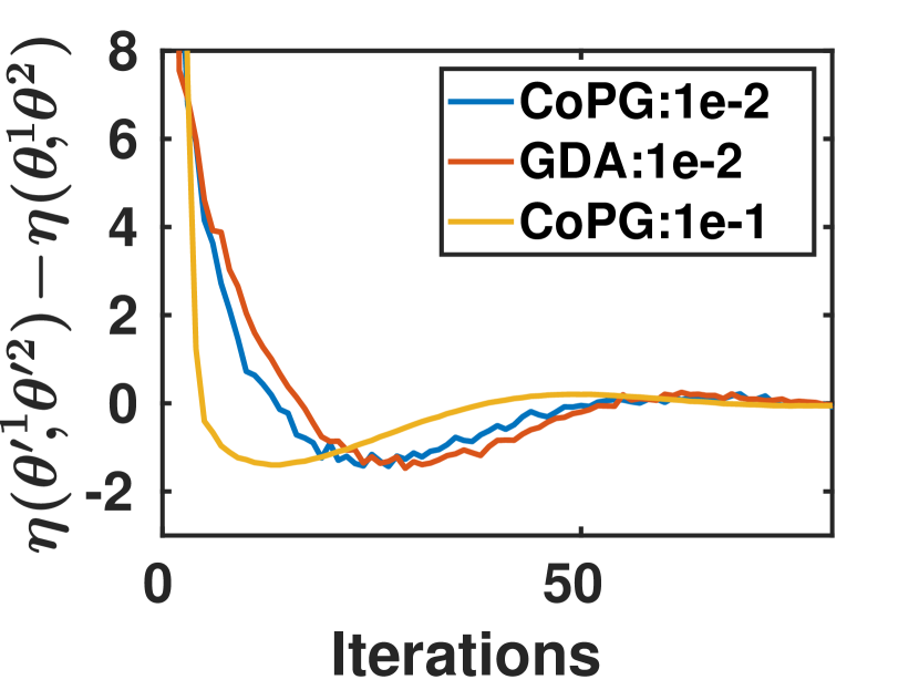
(a)

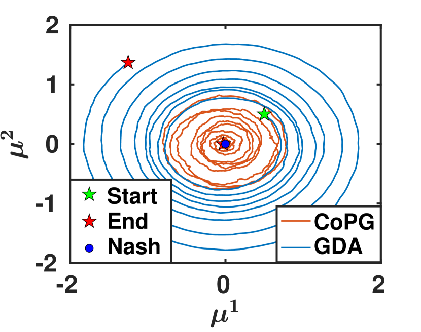
(b)

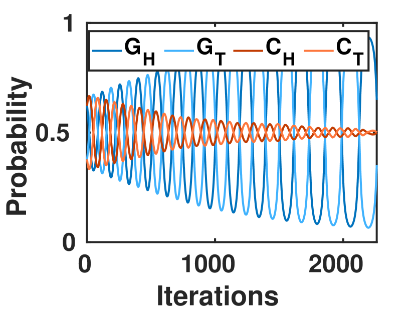
(c)

(d)

Figure 2: During training CoPG (C) vs GDA (G) on a) LQ game, difference in game objective due to policy update for $\alpha=1e-1,1e-2$ b) Bilinear game, $\mu^{1}$ vs $\mu^{2}$ c) MP, probability of selecting Head(H) and Tail(T) d) RPS, probability of selecting rock(R), paper(P) and scissors(S).

Bilinear game is a state-less strongly non-cooperative game, where GDA is known to diverge (Balduzzi et al., 2018). In this game, reward $r(a^{1},a^{2})=\langle{a^{1}},a^{2}\rangle$ where $a^{1}\sim\mathcal{N}(\mu_{1},\sigma_{1})$ and $a^{2}\sim\mathcal{N}(\mu_{2},\sigma_{2})$, and $(\mu_{1},\sigma_{1})$, $(\mu_{2},\sigma_{2})$ are policy parameters. We show that GDA diverges for all learning rates, whereas CoPG converges to the unique Nash equilibrium Fig. 2(b).

Matching pennies and Rock paper scissors, are challenging matrix games with mixed strategies as Nash equilibria, demand opponent aware optimization. We show that CoPG and TRCoPO both converge to the unique Nash equilibrium of MP Fig. 2(c) and RPS Fig. 2(d), whereas GDA and TRGDA diverges (to a sequence of polices that are exploitable by deterministic strategy). Detailed empirical study, formulation and explanation of these four games can be found in Apx. H.

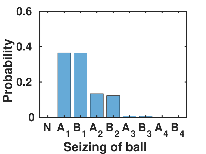
(a) CoPG vs CoPG

(b) GDA vs GDA

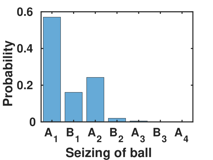
(c) CoPG vs GDA

(d) GDA vs CoPG

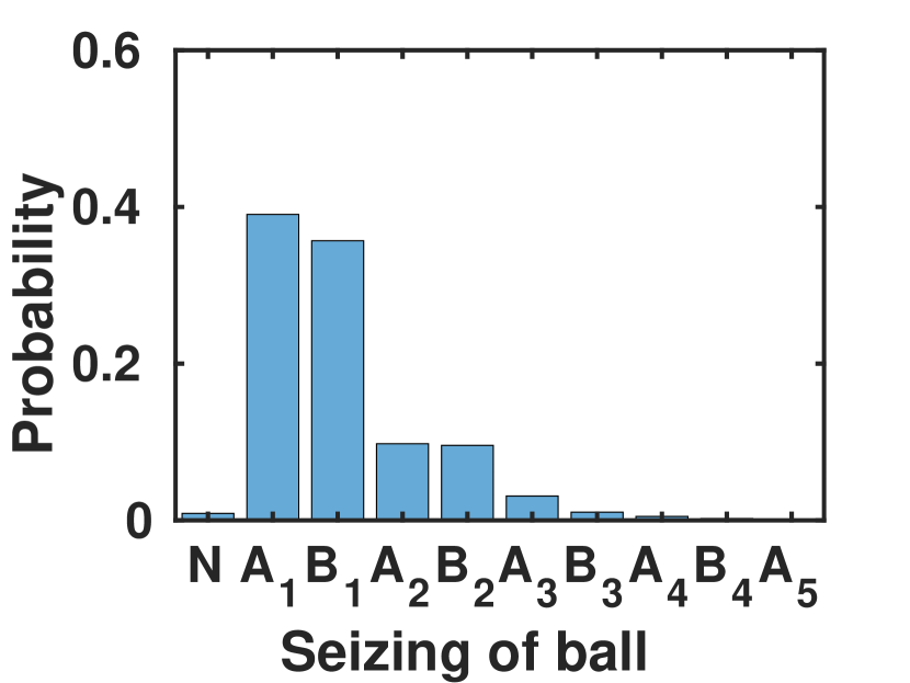
(e) TRCoPO vs TRCoPO

(f) TRGDA vs TRGDA

(g) TRCoPO vs TRGDA

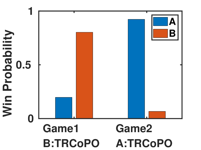
(h) TRGDA vs TRCoPO

Figure 3: a-c), e-g) Interaction plots, representing probability of seizing ball in the game between $A$ vs $B$. X-axis convention, for player $A$. $A_{1}$: $A$ scored goal, $A_{2}$: $A$ scored goal after seizing ball from $B$, $A_{3}$: $A$ scored goal by seizing ball from $B$ which took the ball from $A$ and so forth. Vice versa for player $B$. N: No one scored goal both kept on seizing ball. d),h) probability of games won.

Figure 4: Markov Soccer

Markov soccer game, Fig. 4, consists of players A and B that are randomly initialised in the field, that are supposed to pick up the ball and put it in the opponent’s goal (Littman, 1994; He et al., 2016). The winner is awarded with +1 and the loser with -1 (see Apx. H.5 for more details). Since all methods converge in this game, it is a suitable game to compare learned strategies. In this game, we expect a reasonable player to learn sophisticated strategies of defending, dodging and scoring. For each method playing against their counterparts, e.g., CoPG against CoPG and GDA, Fig. 3 shows the number of times the ball is seized between the players before one player finally scores a goal, or time-out. In (3(a)), CoPG vs CoPG, we see agents seize ball, twice the times as compared to (3(b)),GDA vs GDA (see $A_{2}$ and $B_{2}$ in (3(a)) and (3(b))). In the matches CoPG vs GDA (3(c)), CoPG trained agent could seize the ball from GDA agent ($A_{2}$) nearly 12 times more due to better seizing and defending strategy, but GDA can hardly take the ball back from CoPG ($B_{2}$) due to a better dodging strategy of the CoPG agent. Playing CoPG agent against GDA one, we observe that CoPG wins more than 74% of the games Fig. 3(d). We observe a similar trend for trust region based methods TRCoPO and TRGDA, playing against each other (a slightly stronger results of 85% wins, $A_{2}$ column in Figs 3(g),  3(c)).

We also compared CoPG with MADDPG (Lowe et al., 2017) and LOLA (Foerster et al., 2017a). We observe that the MADDPG learned policy behaves similar to GDA, and loses 80% of the games to CoPG’s (Fig. 14(b)). LOLA learned policy, with its second level reasoning, performs better than GDA, but lose to CoPG 72% of the matches. For completeness, we also compared GDA-PG, CoPG, TRGDA, and TRCoPO playing against each other. TRCoPO performs best,CoPG was runner up, then TRGDA, and lastly GDA (see Apx. H.5).

(a) GDA

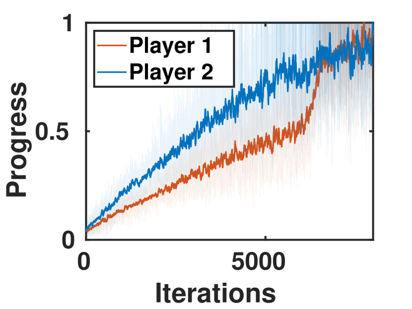
(b) CoPG

(c) TRGDA

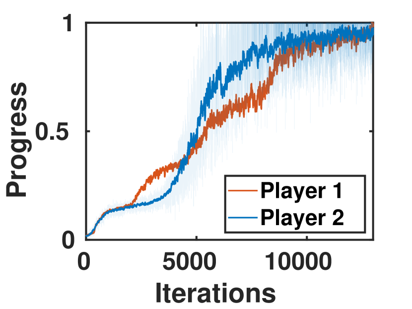
(d) TRCoPO

(e) MADDPG

Figure 5: Normalised progress of agents in one lap of car racing game during training

Car Racing is another interesting game, with continuous state-action space, where two race cars competing against each other to finish the race first Liniger and Lygeros (2020). The game is accompanied by two important challenges, 1) learning a policy that can maneuver the car at the limit of handling, 2) strategic interactions with opponents. The track is challenging, consisting of 13 turns with different curvature (Fig. 13). The game is formulated as a zero-sum, with reward $r(s_{k},a^{1}_{k},a^{2}_{k})=\Delta\rho_{car_{1}}-\Delta\rho_{car_{2}}$, where $\Delta\rho=\rho_{k+1}-\rho_{k}$ and $\rho_{k}$ is the car’s progress along the track at the $k^{th}$ time step. If a car crosses track boundaries (e.g., hit the wall), it is penalized, and the opponent receives rewards, this encourages cars to play rough and push each other into the track boundaries. When a collision happens, the rear car is penalized, and the car in the front receives a reward; it promotes blocking by the car in front and overtaking by the car in the rear.

We study agents trained with all GDA, TRGDA, MADDPG, LOLA, CoPG and TRCoPO in this game, and show that even though all players were able to learn to "drive" only CoPG and TRCoPO were able to learn how to "race". Using GDA, only one player was able to learn, which manifested in either one player completely failing and the other finishing the track (Fig. 5(a)), or by an oscillation behavior where one player learns to go ahead, the other agent stays at lower progress(Fig. 5(c), Fig. 5(e)). Even if one of the players learns to finish one lap at some point, this player does not learn to interact with its opponent(https://youtu.be/rxkGW02GwvE). In contrast, players trained with CoPG and TRGDA, both progress, learn to finish the lap, and race (interact with each other) (See Fig. 5(b) and Fig. 5(d)). To test the policies, we performed races between CoPG and GDA, TRCoPO and TRGDA, and CoPG and TRCoPO. As shown in Tab. 1, CoPG and TRCoPO win almost all races against their counterparts. Overall, we see that both CoPG and TRCoPO are able to learn policies that are faster, more precise, and interactive with the other player (e.g., learns to overtake).

Table 1: Normalized score computed based on 10000 races in the car racing game

	CoPG vs GDA		TRCoPO vs TRGDA		CoPG vs TRCoPO
Wins	1	0	1	0	0.24	0.76
Overtake	1.28	0.78	1.28	0.78	1.80	2.07
Collision	0.17	16.11	0.25	1.87	0.30	0.31

5 Related Work

In tabular CoMDP, Q-learning and actor-critic have been deployed (Littman, 1994, 2001b, 2001a; Greenwald and Hall, 2003; Hu and Wellman, 2003; Grau-Moya et al., 2018; Frénay and Saerens, 2009; Pérolat et al., 2018; Srinivasan et al., 2018), and recently, deep RL methods have been extending to CoMDPs, with focus of modeling agents behaviour (Tampuu et al., 2015; Leibo et al., 2017; Raghu et al., 2017). To mitigate the stabilization issues, centralized methods (Matignon et al., 2012; Lowe et al., 2017; Foerster et al., 2017b), along with opponent’s behavior modeling (Raileanu et al., 2018; He et al., 2016) have been explored. Optimization in multi-agent learning can be interpreted as a game in the parameter space, and the main body of the mentioned literature does not take this aspect directly into account since they attempt to separately improve players’ performance. Hence, they often fail to achieve desirable performance and oftentimes suffer from unstable training, especially in strategic games (Hernandez-Leal et al., 2019; Buşoniu and Babuška, 2010). In imperfect information games with known rules, e.g., poker  (Moravcík et al., 2017), a series of works study algorithmically computing Nash equilibra (Shalev-shwartz and Singer, 2007; Koller et al., 1995; Gilpin et al., 2007; Zinkevich et al., 2008; Bowling et al., 2017). Also, studies in stateless episodic games shown convergence to coarse correlated equilibrium (Hartline et al., 2015; Blum et al., 2008). In contrast CoPO converges to the Nash equilibrium in such games. In two-player competitive games, self-play is an approach of interest where a player plays against itself to improve its behavior (Tesauro, 1995; Silver et al., 2016). But, many of these approaches are limited to specific domains (Heinrich et al., 2015; Heinrich and Silver, 2016).

The closest approach to CoPO in the literature is LOLA (Foerster et al., 2017a) an opponent aware approach. LOLA updates parameters using a second-order correction term, resulting in gradient updates corresponding to the following shortened recursion: if a player thinks that the other player thinks its strategy stays constant (Schäfer and Anandkumar, 2019), whereas CoPO recovers the full recursion series until the Nash equilibrium is delivered. In contrast to  (Foerster et al., 2017a) we also provide CoPO extension to value-based, and trust region-based methods, along with their efficient implementation.

Our work is also related to GANs  (Goodfellow et al., 2014), which involves solving a zero sum two-player competitive game (CoMDP with single state). Recent development in nonconvex-nonconcave problems and GANs training show, simple and intuitive, GDA has undesirable convergence properties  (Mazumdar et al., 2019) and exhibit strong rotation around fixed points  (Balduzzi et al., 2018). To overcome this rotation behaviour of GDA, various modifications have been proposed, including averaging  (Yazıcı et al., 2018), negative momentum  (Gidel et al., 2018) along many others  (Mertikopoulos et al., 2018b; Daskalakis et al., 2017; Mescheder et al., 2017; Balduzzi et al., 2018; Gemp and Mahadevan, 2018). Considering the game-theoretic nature of this problem, competitive gradient descent has been proposed as a natural generalization of gradient descent in two-players instead of GDA for GANs (Schäfer and Anandkumar, 2019). This method, as the predecessor to CoPO, enjoys stability in training, robustness in choice of hyper-parameters, and has desirable performance and convergence properties. This method is also a special case of CoPO when the CoMDP of interest has only one state.

6 Conclusion

We presented competitive policy optimization CoPO, a novel PG-based RL method for two player strictly competitive game. In CoPO, each player optimizes strategy by considering the interaction with the environment and the opponent through game theoretic bilinear approximation to the game objective. This method is instantiated to competitive policy gradient (CoPG) and trust region competitive policy optimisation (TRCoPO) using value based and trust region approaches. We theoretically studied these methods and provided PG theorems to show the properties of these model-free RL approaches. We provided efficient implementation of these methods and empirically showed that they provide stable and faster optimization, and also converge to more sophisticated and competitive strategies. We dedicated this paper to two player zero-sum games, however, the principles provided in this paper can be used for multi-player general games. In the future, we plan to extend this study to multi-player general-sum games along with efficient implementation of methods. Moreover, we plan to use the techniques proposed in partially observable domains, and study imperfect information games (Azizzadenesheli et al., 2020). Also, we aim to explore opponent modelling approaches to relax the requirement of knowing the opponent’s parameters during optimization.

Appendix

Appendix A Algorithms

In this section, we briefly present the algorithms discussed in the paper, namely gradient descent ascent (GDA), competitive policy gradient (CoPG), trust region gradient descent ascent (TRGDA) and trust region competitive policy optimization (TRCoPO).

Initialize $(\theta^{1},\theta^{2})$

for $epoch:1,2,3,..$ until termination do

       Collect samples under $\pi(.|.;\theta^{1})$, $\pi(.|.;\theta^{2})$,

       Estimate $Q$, then $D_{\theta^{i}}\eta$ in Eq.7

       Update $\theta^{1},\theta^{2}$ using Eq. 4

      

end for

Algorithm 1 Gradient Descent Ascent Policy Gradient

Initialize $(\theta^{1},\theta^{2})$

for $epoch:1,2,3,..$ until termination do

       Collect samples under $\pi(.|.;\theta^{1})$, $\pi(.|.;\theta^{2})$,

       Estimate $Q$, then $D_{\theta^{i}}\eta,D_{\theta^{i}\theta^{j}}\eta$ in Eqs. 7,8

       Update $\theta^{1},\theta^{2}$ using Eq. 3

      

end for

Algorithm 2 Competitive Policy Gradient

Initialize $(\theta^{1},\theta^{2})$

for $epoch:1,2,3,..$ until termination do

       Collect samples under $\pi(.|.;\theta^{1})$, $\pi(.|.;\theta^{2})$,

       Estimate $A$, and $D_{\theta^{i}}L$ using Eq. F.3,

       Update $\theta^{i}$ using Eq. F.3, with bilinear term as a null matrix.

      

end for

Algorithm 3 Trust Region Gradient Descent Ascent

Initialize $(\theta^{1},\theta^{2})$

for $epoch:1,2,3,..$ until termination do

       Collect samples under $\pi(.|.;\theta^{1})$, $\pi(.|.;\theta^{2})$,

       Estimate $A$, and $D_{\theta^{i}}L,D_{\theta^{i}\theta^{j}}L$ using Eq. F.3,

       Update $\theta^{1},\theta^{2}$ using Eq. F.3,

      

end for

Algorithm 4 Trust Region Competitive Policy Optimisation

Appendix B Recursion reasoning

When players play strategic games, in order to maximize their payoffs, they need to consider their opponents’ strategies which in turn may depend on their strategies (and so on), resulting in the well known infinite recursion in game theory. This is the recursive reasoning of the form what do I think that you think that I think (and so on) and arises while acting rationally in multi-player games. In this section we elaborate on the recursion in CoMDP and latter show how CoPO recovers the infinite recursion reasoning Fig. 6. Recursion reasoning in CoMDP works as follows:

• Level 1 recursion: Each player considers how the environment, as the results of the agents’ current and future moves temporally evolves in favor of each agent,

• Level 2 recursion: Considering that the other agent also considers how the environment, as the results of the agents’ current and future moves temporally evolves in favor of each agent,

• Level 3 recursion: Considering that the other agent also considers that the other agent also considers how the environment, as the results of the agents’ current and future moves temporally evolves in favor of each agent,

• …….

Figure 6: Recursion reasoning. The notion of "Level N recursion" in the figure assumes that there is no further recursive thinking (cloud) beyond that level.

In the special case of single state games (non sequential setting), this recursive reasoning boils down to what each player thinks, the other player thinks that the other player thinks, …. . ( For readers interested in the recursion reasoning in non-sequential but repeated episodic competitive games (single state (or stateless) episodic CoMDP), stability and convergence of competitive gradient optimization and the derivation of Eq. 3, we refer to [Schäfer and Anandkumar, 2019]).

In the following we provide an intuitive explanation for the updates prescribed by CoPO. Let us restate the Nash equilibrium of the bilinear game in Eq. 3 in its matrix form,

$$\begin{bmatrix}\theta^{1}\\ \theta^{2}\\ \end{bmatrix}\leftarrow\begin{bmatrix}\theta^{1}\\ \theta^{2}\\ \end{bmatrix}+\alpha\begin{bmatrix}I&-\alpha D_{\theta^{1}\theta^{2}}\eta\\ \alpha D_{\theta^{2}\theta^{1}}\eta&I\\ \end{bmatrix}^{-1}\begin{bmatrix}D_{{\theta}^{1}}\eta\\ -D_{{\theta}^{2}}\eta\\ \end{bmatrix}.$$ (13)

We rewrite the above mentioned update as

$$\begin{bmatrix}\theta^{1}\\ \theta^{2}\\ \end{bmatrix}\leftarrow\begin{bmatrix}\theta^{1}\\ \theta^{2}\\ \end{bmatrix}+\alpha(I-A)^{-1}\begin{bmatrix}D_{{\theta}^{1}}\eta\\ -D_{{\theta}^{2}}\eta\\ \end{bmatrix},\quad\text{with }\quad A=\begin{bmatrix}0&\alpha D_{\theta^{1}\theta^{2}}\eta\\ -\alpha D_{\theta^{2}\theta^{1}}\eta&0\\ \end{bmatrix}.$$ (14)

If it holds that the spectral radius of $A$ is smaller than one, then we can use the Neumann series to compute the inverse,

$$(I-A)^{-1}=\lim_{N\rightarrow\infty}\sum_{k=0}^{N}A^{k}=I+A+A^{2}+A^{3}+...\,.$$ (15)

Using this expansion and its different orders as an approximation, e.g., up to $k\in\{0,\ldots,N\}$ for a finite $N$, we derive policy update rules that have different levels of reasoning. For example, consider the following levels of recursion reasoning:

• N = 0, $(I-A)^{-1}\rightarrow I$, i.e., we approximate $(I-A)^{-1}$ with the first term in the series presented in Eq. 15, therefore, the update rule in Eq. 13 reduces to the GDA update rule. In this case, each agent updates its parameters considering its current and future moves to gain a higher total cumulative reward in the environment assuming the policy of the opponent stays unchanged,

  $$\begin{bmatrix}\theta^{1}\\ \theta^{2}\\ \end{bmatrix}\leftarrow\begin{bmatrix}\theta^{1}\\ \theta^{2}\\ \end{bmatrix}+\alpha\begin{bmatrix}D_{{\theta}^{1}}\eta\\ -D_{{\theta}^{2}}\eta\\ \end{bmatrix}.$$

• N = 1, $(I-A)^{-1}\rightarrow I+A$ and the update rule in Eq. 13 reduce to the LOLA update rule. In this case, each agent updates its parameters considering that the opponent updates its parameters considering the other player stays unchanged. For example, player $1$ updates its parameter, assuming that player $2$ also updates its parameter, but player $1$ assumes that the player $2$ updates its parameter assuming the player $1$ stays unchanged.

  $$\begin{bmatrix}\theta^{1}\\ \theta^{2}\\ \end{bmatrix}\leftarrow\begin{bmatrix}\theta^{1}\\ \theta^{2}\\ \end{bmatrix}+\alpha\begin{bmatrix}D_{{\theta}^{1}}\eta-\alpha D_{\theta^{1}\theta^{2}}\eta D_{\theta^{2}}\eta\\ -D_{{\theta}^{2}}\eta-\alpha D_{\theta^{2}\theta^{1}}\eta D_{\theta^{1}}\eta\\ \end{bmatrix}.$$

• N = 2, $(I-A)^{-1}\rightarrow I+A+A^{2}$, and the update rule is given by Eq. 16. In this case, the agent updates its parameters considering that the opponent also considering that the agent is considering to update parameters, such that its current and future moves increase the probability of earning a higher total cumulative reward in the environment.

  $$\begin{bmatrix}\theta^{1}\\ \theta^{2}\\ \end{bmatrix}\leftarrow\begin{bmatrix}\theta^{1}\\ \theta^{2}\\ \end{bmatrix}+\alpha\begin{bmatrix}D_{{\theta}^{1}}\eta-\alpha D_{\theta^{1}\theta^{2}}\eta D_{\theta^{2}}\eta-\alpha^{2}D_{\theta^{1}\theta^{2}}\eta D_{\theta^{2}\theta^{1}}\eta D_{\theta^{1}}\eta\\ -D_{{\theta}^{2}}\eta-\alpha D_{\theta^{2}\theta^{1}}\eta D_{\theta^{1}}\eta+\alpha^{2}D_{\theta^{2}\theta^{1}}\eta D_{\theta^{1}\theta^{2}}\eta D_{\theta^{2}}\eta\\ \end{bmatrix}.$$ (16)

• $\lim$ N $\rightarrow$ $\infty$, $(I-A)^{-1}\rightarrow I+A+A^{2}+A^{3}+...$, we recover the Nash equilibrium in the limit which corresponds to infinite recursion reasoning. In this case, the update rule in Eq. 13 is given by Eq. 17 which resembles the Eq. 3.

  $$\begin{bmatrix}\theta^{1}\\ \theta^{2}\end{bmatrix}\leftarrow\begin{bmatrix}\theta^{1}\\ \theta^{2}\end{bmatrix}+\alpha\begin{bmatrix}\bigl{(}Id+\alpha^{2}D_{\theta^{1}\theta^{2}}\eta D_{\theta^{2}\theta^{1}}\eta\bigr{)}^{-1}\bigl{(}D_{\theta^{1}}\eta-\alpha D_{\theta^{1}\theta^{2}}\eta D_{\theta^{2}}\eta\bigr{)}\\ -\bigl{(}Id+\alpha^{2}D_{\theta^{2}\theta^{1}}\eta D_{\theta^{1}\theta^{2}}\eta\bigr{)}^{-1}\bigl{(}D_{\theta^{2}}\eta+\alpha D_{\theta^{2}\theta^{1}}\eta D_{\theta^{1}}\eta\bigr{)}\\ \end{bmatrix}.$$ (17)

We provided this discussion to motivate the importance of taking the game theoretic nature of a given problem into account, in order to design an update.

Appendix C Proof of competitive policy gradient theorem

In this section, we first derive the gradient and bilinear terms in the form of score function. In the subsequent subsections we provide complete proof of the competitive policy gradient theorem.

C.1 Proof for Prop. 1:

Proof.

Given that the agents’ policies are parameterized with $\theta^{1}$ and $\theta^{2}$, we know that the game objective is,

$$\eta(\theta^{1},\theta^{2}) =\int_{\tau}f(\tau;\theta^{1},\theta^{2})R(\tau)d\tau,$$ (18)

thus, the gradient with respect to $$\theta_{i}$$ is given by

$$D_{\theta^{i}}\eta =\int_{\tau}D_{\theta_{i}}f(\tau;\theta^{1},\theta^{2})R(\tau)d\tau,\;i\in\!\{1,2\}\,,$$ (19)

for any $$p_{\theta}(\tau)\neq 0 D_{\theta}\log p_{\theta}(\tau)=\frac{D_{\theta}p_{\theta}(\tau)}{p_{\theta}(\tau)} f(\tau;\theta^{1},\theta^{2})$$ using from standard calculus and the definition of in Eq. 1, we can compute the gradient of the game objective,

$$D_{\theta^{i}}\eta =\int_{\tau}f(\tau;\theta^{1},\theta^{2})(D_{\theta^{i}}\log(\prod_{k=0}^{|\tau|-1}\pi(a_{k}|s_{k};\theta^{i})))R(\tau)d\tau\,,$$

Let us define the score function as $$g(\tau,\theta^{i})=D_{\theta^{i}}(\log(\prod_{k=0}^{|\tau|-1}\pi(a_{k}|s_{k};\theta^{i})))$$ which results in,

$$D_{\theta^{i}}\eta =\int_{\tau}f(\tau;\theta^{1},\theta^{2})g(\tau,\theta^{i})R(\tau)d\tau.$$ (20)

By definition we know that the second order bilinear approximation of the game objective is $$D_{\theta^{2}\theta^{1}}\eta(\theta^{1},\theta^{2})=D_{\theta^{2}}D_{\theta^{1}}\eta(\theta^{1},\theta^{2})$$. Hence,

$$D_{\theta^{2}\theta^{1}}\eta =\int_{\tau}D_{\theta^{2}}f(\tau;\theta^{1},\theta^{2})g(\tau,\theta^{1})^{\top}R(\tau)d\tau\,.$$

$$=\int_{\tau}f(\tau;\theta^{1},\theta^{2})(D_{\theta^{2}}\log(\prod_{k=0}^{|\tau|-1}\pi(a_{k}|s_{k};\theta^{2})))g(\tau,\theta^{1})^{\top}R(\tau)d\tau\,,$$

$$=\int_{\tau}f(\tau;\theta^{1},\theta^{2})g(\tau,\theta^{2})g(\tau,\theta^{1})^{\top}R(\tau)d\tau\,.$$

which concludes the proof. ∎

C.2 Proof for Thm. 1

The competitive policy gradient theorem (Thm. 1) consists of two parts. We first provide the derivation for the gradient and utilise this result to derive the bilinear term in the subsequent subsection.

C.2.1 Derivation of gradient term $D_{\theta^{1}}\eta$

Proof.

Using Eq. 2, which defines $V(s_{k};\theta^{1},\theta^{2})$ and $Q(s_{k},a^{1}_{k},a^{2}_{k};\theta^{1},\theta^{2})$. We can write $V(s_{0};\theta^{1},\theta^{2})$ as,

$$V(s_{0};\theta^{1},\theta^{2}) =\!\int_{a_{0}^{1}}\!\int_{a_{0}^{2}}\!\!\!\pi(a_{0}^{1}|s_{0};\theta^{1})\pi(a_{0}^{2}|s_{0};\theta^{2})Q(s_{0},a_{0}^{1},a_{0}^{2};\theta^{1}\!\!,\theta^{2})da_{0}^{1}da_{0}^{2}\,,$$ (21)

$$\text{where, }\,Q(s_{0},a_{0}^{1},a_{0}^{2};\theta^{1}\!\!,\theta^{2}) =r(s_{0},a_{0}^{1},a_{0}^{2})+\gamma\int_{s_{1}}T(s_{1}|s_{0},a_{0}^{1},a_{0}^{2})V(s_{0};\theta^{1},\theta^{2})ds_{1}\,.$$

Hence, the gradient of the state-value $$V$$ is,

$$D_{\theta^{1}}V(s_{0};\theta^{1},\theta^{2}) =\int_{a_{0}^{1}}\int_{a_{0}^{2}}\frac{\partial\pi(a_{0}^{1}|s_{0};\theta^{1})}{\partial\theta^{1}}\pi(a_{0}^{2}|s_{0};\theta^{2})Q(s_{0},a_{0}^{1},a_{0}^{2};\theta^{1}\!\!,\theta^{2})da_{0}^{1}da_{0}^{2}$$

$$+\!\!\int_{a_{0}^{1}}\!\int_{a_{0}^{2}}\!\!\pi(a_{0}^{1}|s_{0};\theta^{1})\pi(a_{0}^{2}|s_{0};\theta^{2})\!\frac{\partial Q(s_{0},a_{0}^{1},a_{0}^{2};\theta^{1}\!\!,\theta^{2})}{\partial\theta^{1}}da_{0}^{1}da_{0}^{2}.$$ (22)

The gradient of the state-action value $$Q V$$, in term of the gradient of the state-value is given by

$$D_{\theta^{1}}Q(s_{0},a_{0}^{1},a_{0}^{2};\theta^{1}\!\!,\theta^{2}) =\gamma\int_{s_{1}}T(s_{1}|s_{0},a_{0}^{1},a_{0}^{2})\frac{\partial V(s_{1};\theta^{1},\theta^{2})}{\partial\theta^{1}}ds_{1}\,.$$ (23)

Substituting Eq. 23 in Eq. C.2.1 results in,

$$\!D_{\theta^{1}}\!V(\!s_{0};\theta^{1},\theta^{2}) =\!\int_{a_{0}^{1}}\!\!\int_{a_{0}^{2}}\!\!\!\!\frac{\partial\pi(\!a_{0}^{1}|s_{0};\theta^{1})}{\partial\theta^{1}}\pi(\!a_{0}^{2}|s_{0};\theta^{2})Q(\!s_{0},a_{0}^{1},a_{0}^{2};\theta^{1}\!\!,\theta^{2})da_{0}^{1}da_{0}^{2}$$ (24)

$$+\!\int_{a_{0}^{1}}\!\!\int_{a_{0}^{2}}\!\!\!\!\pi(a_{0}^{1}|s_{0};\theta^{1})\pi(a_{0}^{2}|s_{0};\theta^{2})\gamma\!\!\int_{s_{1}}\!\!\!\!T(s_{1}|s_{0},a_{0}^{1},a_{0}^{2})\frac{\partial V(s_{1};\theta^{1},\theta^{2})}{\partial\theta^{1}}ds_{1}da_{0}^{1}da_{0}^{2}\,.$$

By exploring the recursive nature of the state-value $$V D_{\theta^{1}}V(s_{0};\theta^{1},\theta^{2})$$ and , we can unroll Eq. 24 as,

$$\!D_{\theta^{1}}\!V(s_{0};\theta^{1},\theta^{2}) =\int_{a_{0}^{1}}\int_{a_{0}^{2}}\frac{\partial\pi(a_{0}^{1}|s_{0};\theta^{1})}{\partial\theta^{1}}\pi(a_{0}^{2}|s_{0};\theta^{2})Q(s_{0},a_{0}^{1},a_{0}^{2};\theta^{1},\theta^{2})da_{0}^{1}da_{0}^{2}$$ (25)

$$+\int_{a_{0}^{1}}\int_{a_{0}^{2}}\pi(a_{0}^{1}|s_{0};\theta^{1})\pi(a_{0}^{2}|s_{0};\theta^{2})\gamma\int_{s_{1}}T(s_{1}|s_{0},a_{0}^{1},a_{0}^{2})$$

$$\quad\quad\Biggl{(}\int_{a_{1}^{1}}\int_{a_{1}^{2}}\frac{\partial\pi(a_{1}^{1}|s_{1};\theta^{1})}{\partial\theta^{1}}\pi(a_{1}^{2}|s_{1};\theta^{2})Q(s_{1},a_{1}^{1},a_{1}^{2};\theta^{1},\theta^{2})da_{1}^{1}da_{1}^{2}$$

$$\quad\quad\quad\quad\quad+\int_{a_{1}^{1}}\int_{a_{1}^{2}}\pi(a_{1}^{1}|s_{1};\theta^{1})\pi(a_{1}^{2}|s_{1};\theta^{2})\gamma\int_{s_{2}}T(s_{2}|s_{1},a_{1}^{1},a_{1}^{2})$$

$$\ \ \quad\quad\quad\quad\quad\quad\quad\quad\quad\quad\quad\quad\frac{\partial V(s_{2};\theta^{1},\theta^{2})}{\partial\theta^{1}}ds_{2}da_{1}^{1}da_{1}^{2}\Biggr{)}ds_{1}da_{0}^{1}da_{0}^{2}\,.$$

To find the derivative of the expected return, we can use the definition of the expected return $$\eta(\theta^{1},\theta^{2})$$ and Eq. 25, which results in

$$\!\!\!\!\!\!\!\!\!\!D_{\theta^{1}}\eta(\theta^{1},\theta^{2}) =\!\int_{s_{0}}p(s_{0})D_{\theta^{1}}V(s_{0};\theta^{1},\theta^{2})ds_{0}$$

$$=\! \int_{s_{0}}p(s_{0})\int_{a_{0}^{1}}\int_{a_{0}^{2}}\frac{\partial\pi(a_{0}^{1}|s_{0};\theta^{1})}{\partial\theta^{1}}\pi(a_{0}^{2}|s_{0};\theta^{2})Q(s_{0},a_{0}^{1},a_{0}^{2};\theta^{1}\!\!,\theta^{2})da_{0}^{1}da_{0}^{2}ds_{0}$$

$$+\!\gamma\!\!\int_{\tau}\!\!f(\tau_{0:0},s_{1};\theta^{1}\!\!,\theta^{2})\frac{\partial\!\pi(a_{1}^{1}|s_{1};\theta^{1})}{\partial\theta^{1}}\pi(a_{1}^{2}|s_{1};\theta^{2})Q(s_{1},a_{1}^{1},a_{1}^{2};\theta^{1}\!\!,\theta^{2})d\tau_{0:1}$$

$$+\gamma^{2}\int_{\tau}f(\tau_{0:1},s_{2};\theta^{1},\theta^{2})\frac{\partial V(s_{2};\theta^{1},\theta^{2})}{\partial\theta^{1}}ds_{2}d\tau_{0:1}.$$ (26)

Similar to the two previous step, unrolling and marginalisation can be continued for the entire length of the trajectory, which results in,

$$\!\!\!\!\!\!\!\!\!\!D_{\theta^{1}}\eta(\theta^{1},\theta^{2})=\!\int_{\tau} \!\sum_{k=0}^{|\tau|-1}\!\!\!\gamma^{k}\!f(\!\tau_{0:k-1}\!,\!s_{k}\!;\theta^{1}\!\!,\theta^{2})\!\!\!\int_{a_{k}^{1}}\!\!\int_{a_{k}^{2}}\!\!\!\!\!\frac{\partial\pi(\!a_{k}^{1}|s_{k};\!\theta^{1}\!)}{\partial\theta^{1}}\!\pi(\!a_{k}^{2}|s_{k};\!\theta^{2})Q(\!s_{k},\!a_{k}^{1},\!a_{k}^{2};\!\theta^{1}\!\!,\theta^{2})d\tau$$ (27)

$$=\int_{\tau} \sum_{k=0}^{|\tau|-1}\!\!\gamma^{k}\!f(\tau_{0:k};\theta^{1},\theta^{2})\frac{\partial\log\pi(a_{k}^{1}|s_{k};\theta^{1})}{\partial\theta^{1}}Q(s_{k},a_{k}^{1},a_{k}^{2};\theta^{1}\!\!,\theta^{2})d\tau.$$ (28)

This concludes our derivation of the gradient term of the game objective for the two agent case. ∎

C.2.2 Derivation of Bilinear term $D_{\theta^{1}\theta^{2}}\eta$

Proof: By definition we know that $D_{\theta^{1}\theta^{2}}V(s_{0};\theta^{1},\theta^{2})=D_{\theta^{1}}(D_{\theta^{2}}V(s_{0};\theta^{1},\theta^{2}))$. Thus we can use $D_{\theta^{2}}V(s_{0};\theta^{1},\theta^{2})$ as defined in Eq. C.2.1 and differentiating with respect to $\theta^{1}$, thereby we get,

$$D_{\theta^{1}\theta^{2}}V(s_{0};\theta^{1},\theta^{2}) =\int_{a_{0}^{1}}\int_{a_{0}^{2}}\frac{\partial\pi(a_{0}^{1}|s_{0};\theta^{1})}{\partial\theta^{1}}\frac{\partial\pi(a_{0}^{2}|s_{0};\theta^{2})}{\partial\theta^{2}}^{\top}Q(s_{0},a_{0}^{1},a_{0}^{2};\theta^{1}\!\!,\theta^{2})da_{0}^{1}da_{0}^{2}$$

$$+\int_{a_{0}^{1}}\int_{a_{0}^{2}}\frac{\partial\pi(a_{0}^{1}|s_{0};\theta^{1})}{\partial\theta^{1}}\pi(a_{0}^{2}|s_{0};\theta^{2})\frac{\partial Q(s_{0},a_{0}^{1},a_{0}^{2};\theta^{1}\!\!,\theta^{2})}{\partial\theta^{2}}^{\top}da_{0}^{1}da_{0}^{2}$$

$$+\int_{a_{0}^{1}}\int_{a_{0}^{2}}\pi(a_{0}^{1}|s_{0};\theta^{1})\frac{\partial Q(s_{0},a_{0}^{1},a_{0}^{2};\theta^{1}\!\!,\theta^{2})}{\partial\theta^{1}}\frac{\partial\pi(a_{0}^{2}|s_{0};\theta^{2})}{\partial\theta^{2}}^{\top}da_{0}^{1}da_{0}^{2}$$

$$+\int_{a_{0}^{1}}\int_{a_{0}^{2}}\pi(a_{0}^{1}|s_{0};\theta^{1})\pi(a_{0}^{2}|s_{0};\theta^{2})\frac{\partial^{2}Q(s_{0},a_{0}^{1},a_{0}^{2};\theta^{1}\!\!,\theta^{2})}{\partial\theta^{1}\partial\theta^{2}}da_{0}^{1}da_{0}^{2}.$$ (29)

Exploiting the recursive structure of $D_{\theta^{1}\theta^{2}}V(s_{0};\theta^{1},\theta^{2})$, we can evaluate $D_{\theta^{1}\theta^{2}}V(s_{1};\theta^{1},\theta^{2})$ and substitute it back in Eq. 29,we get,

$$D_{\theta^{1}\theta^{2}}V(s_{0};\theta^{1},\theta^{2})= \int_{a_{0}^{1}}\int_{a_{0}^{2}}\frac{\partial\pi(a_{0}^{1}|s_{0};\theta^{1})}{\partial\theta^{1}}\frac{\partial\pi(a_{0}^{2}|s_{0};\theta^{2})}{\partial\theta^{2}}^{\top}Q(s_{0},a_{0}^{1},a_{0}^{2};\theta^{1}\!\!,\theta^{2})da_{0}^{1}da_{0}^{2}$$ (30)

$$+\int_{a_{0}^{1}}\int_{a_{0}^{2}}\frac{\partial\pi(a_{0}^{1}|s_{0};\theta^{1})}{\partial\theta^{1}}\pi(a_{0}^{2}|s_{0};\theta^{2})\frac{\partial Q(s_{0},a_{0}^{1},a_{0}^{2};\theta^{1}\!\!,\theta^{2})}{\partial\theta^{2}}^{\top}da_{0}^{1}da_{0}^{2}$$

$$+\int_{a_{0}^{1}}\int_{a_{0}^{2}}\pi(a_{0}^{1}|s_{0};\theta^{1})\frac{\partial Q(s_{0},a_{0}^{1},a_{0}^{2};\theta^{1}\!\!,\theta^{2})}{\partial\theta^{1}}\frac{\partial\pi(a_{0}^{2}|s_{0};\theta^{2})}{\partial\theta^{2}}^{\top}da_{0}^{1}da_{0}^{2}$$

$$+\int_{a_{0}^{1}}\!\int_{a_{0}^{2}}\!\!\!\pi(a_{0}^{1}|s_{0};\theta^{1})\pi(a_{0}^{2}|s_{0};\theta^{2})\Biggl{(}\!\!\gamma\!\!\int_{s_{1}}\!\!T(s_{1}|s_{0},a_{0}^{1},a_{0}^{2})\!$$

$$\quad\quad\biggl{(}\!\int_{a_{1}^{1}}\!\!\int_{a_{1}^{2}}\!\!\frac{\partial\pi(a_{1}^{1}|s_{1};\theta^{1}\!)}{\partial\theta^{1}}\frac{\partial\pi(a_{1}^{2}|s_{1};\theta^{2}\!)}{\partial\theta^{2}}^{\top}Q(s_{1},a_{1}^{1},a_{1}^{2};\theta^{1}\!,\theta^{2}\!)da_{1}^{1}da_{1}^{2}$$

$$+\int_{a_{1}^{1}}\int_{a_{1}^{2}}\frac{\partial\pi(a_{1}^{1}|s_{1};\theta^{1})}{\partial\theta^{1}}\pi(a_{1}^{2}|s_{1};\theta^{2})\frac{\partial Q(s_{1},a_{1}^{1},a_{1}^{2};\theta^{1}\!\!,\theta^{2})}{\partial\theta^{2}}^{\top}da_{1}^{1}da_{1}^{2}$$

$$+\int_{a_{1}^{1}}\int_{a_{1}^{2}}\pi(a_{1}^{1}|s_{1};\theta^{1})\frac{\partial Q(s_{1},a_{1}^{1},a_{1}^{2};\theta^{1}\!\!,\theta^{2})}{\partial\theta^{1}}\frac{\partial\pi(a_{1}^{2}|s_{1};\theta^{2})}{\partial\theta^{2}}^{\top}da_{1}^{1}da_{1}^{2}$$

$$\!\!\!\!\!\!\!\!\!\!\!\!\!\!\!\!\!\!\!\!\!\!\!\!\!\!\!\!\!\!\!\!\!\!\!\!\!\!\!\!\!\!\!\!\!\!\!+\!\int_{a_{1}^{1}}\!\!\int_{a_{1}^{2}}\!\!\!\pi(a_{1}^{1}|s_{1};\theta^{1})\pi(a_{1}^{2}|s_{1};\theta^{2})\!\gamma\!\!\int_{s_{2}}\!\!\!\!T(s_{2}|s_{1},a_{1}^{1},a_{1}^{2})\frac{\partial^{2}V(s_{2};\theta^{1},\theta^{2})}{\partial\theta^{2}\partial\theta^{1}}ds_{2}da_{1}^{1}da_{1}^{2}\!\biggr{)}ds_{1}\!\!\!\Biggr{)}da_{0}^{1}da_{0}^{2}.$$

Exploring the recursive structure, quickly leads to long sequences of terms, to deal with this let us define a short hand notation, the first term in Eq. 29 is denoted by $b_{0}$, second term by $c_{0}$, third term by $d_{0}$, forth term as $e_{0}$, note that the subscript indicates the time step and let $Pr_{k}=Pr(s_{k}\rightarrow s_{k+1},\theta^{1},\theta^{2})$ be the state transition probability summed over all actions. When investigating Eq. 30 note that the forth term of Eq. 29 $e_{0}$, expanded to $e_{0}=\gamma\int_{s_{1}}Pr_{0}(b_{1}+c_{1}+d_{1}+e_{1})ds_{1}$. Thus, recursively applying this insight and using our short hand notation results in,

$$D_{\theta^{1}\theta^{2}}V(s_{0};\theta^{1},\theta^{2})= b_{0}\!+\!c_{0}\!+\!d_{0}\!+\!\gamma\int_{s_{1}}\!\!Pr_{0}\Bigl{(}\!b_{1}\!+\!c_{1}\!+\!d_{1}\!+\!\gamma\int_{s_{2}}\!\!Pr_{1}\Bigl{(}\!b_{2}\!+\!c_{2}\!+\!d_{2}$$

$$\!+\!\gamma\int_{s_{3}}\!\!Pr_{2}\Bigl{(}\!b_{3}\!+\!c_{3}\!+\!d_{3}\!+\!\gamma\int_{s_{4}}\!\!Pr_{3}\Bigl{(}\!...\!\Bigr{)}ds_{4}\!\Bigr{)}ds_{3}\!\Bigr{)}ds_{2}\!\Bigr{)}ds_{1}$$

$$= b_{0}\!+\!\gamma\!\!\int_{s_{1}}\!\!Pr_{0}\Bigl{(}\!b_{1}\!+\!\gamma\!\!\int_{s_{2}}\!\!Pr_{1}\Bigl{(}\!b_{2}\!+\!\gamma\!\!\int_{s_{3}}\!\!Pr_{2}\Bigl{(}\!b_{3}\!+\!\gamma\!\!\int_{s_{4}}\!\!Pr_{3}\Bigl{(}\!...\!\Bigr{)}ds_{4}\!\Bigr{)}ds_{3}\!\Bigr{)}ds_{2}\!\Bigr{)}ds_{1}$$

$$\!\!\!\!\!\!\!\!\!+\!c_{0}\!+\!\gamma\!\!\int_{s_{1}}\!\!Pr_{0}\Bigl{(}\!c_{1}\!+\!\gamma\!\!\int_{s_{2}}\!\!Pr_{1}\Bigl{(}\!c_{2}\!+\!\gamma\int_{s_{3}}\!\!Pr_{2}\Bigl{(}\!c_{3}\!+\!\gamma\!\!\int_{s_{4}}\!\!Pr_{3}\Bigl{(}\!...\!\Bigr{)}ds_{4}\!\Bigr{)}ds_{3}\!\Bigr{)}ds_{2}\!\Bigr{)}ds_{1}$$

$$\!\!\!\!\!\!\!\!\!+\!d_{0}\!+\!\gamma\!\!\int_{s_{1}}\!\!Pr_{0}\Bigl{(}\!d_{1}\!+\!\gamma\!\!\int_{s_{2}}\!\!Pr_{1}\Bigl{(}\!d_{2}\!+\!\gamma\!\!\int_{s_{3}}\!\!Pr_{2}\Bigl{(}\!d_{3}\!+\!\gamma\!\!\int_{s_{4}}\!\!Pr_{3}\Bigl{(}\!...\!\Bigr{)}ds_{4}\!\Bigr{)}ds_{3}\!\Bigr{)}ds_{2}\!\Bigr{)}ds_{1}.$$

Summing over the initial state distribution results in,

$$\!\!D_{\theta^{1}\theta^{2}}\eta(\theta^{1},\theta^{2})\! =\!\!\int_{s_{0}}\!\!\!\!p(s_{0})D_{\theta^{1}\theta^{2}}V(s_{0};\theta^{1},\theta^{2})ds_{0}$$

$$\!\!\!\!\!\!\!\!\!\!\!\!\!\!\!\!\!\!\!\!=\!\!\int_{s_{0}}\!\!\!\!p(s_{0})\Bigl{(}\!b_{0}\!\!+\!\!\gamma\!\!\int_{s_{1}}\!\!\!\!Pr_{0}\Bigl{(}\!b_{1}\!\!+\!\!\gamma\!\!\int_{s_{2}}\!\!\!\!Pr_{1}\Bigl{(}\!b_{2}\!\!+\!\!\gamma\!\!\int_{s_{3}}\!\!\!\!Pr_{2}\Bigl{(}\!b_{3}\!\!+\!\!\gamma\!\!\int_{s_{4}}\!\!\!\!Pr_{3}\Bigl{(}\!...\!\Bigr{)}ds_{4}\!\Bigr{)}ds_{3}\!\Bigr{)}ds_{2}\!\Bigr{)}ds_{1}\!\Bigr{)}ds_{0}$$

$$\quad\!\!\!\!\!\!\!\!\!\!\!\!\!\!\!\!\!\!\!\!+\!\!\!\int_{s_{0}}\!\!\!\!p(s_{0})\Bigl{(}\!c_{0}\!\!+\!\!\gamma\!\!\int_{s_{1}}\!\!\!\!Pr_{0}\Bigl{(}\!c_{1}\!\!+\!\!\gamma\!\!\int_{s_{2}}\!\!\!\!Pr_{1}\Bigl{(}\!c_{2}\!\!+\!\!\gamma\!\!\int_{s_{3}}\!\!\!\!Pr_{2}\Bigl{(}\!c_{3}\!\!+\!\!\gamma\!\!\int_{s_{4}}\!\!\!\!Pr_{3}\Bigl{(}\!...\!\Bigr{)}ds_{4}\!\Bigr{)}ds_{3}\!\Bigr{)}ds_{2}\!\Bigr{)}ds_{1}\!\Bigr{)}ds_{0}$$

$$\quad\!\!\!\!\!\!\!\!\!\!\!\!\!\!\!\!\!\!\!\!+\!\!\!\int_{s_{0}}\!\!\!\!\!p(s_{0})\Bigl{(}\!d_{0}\!\!+\!\!\gamma\!\!\int_{s_{1}}\!\!\!\!\!Pr_{0}\Bigl{(}\!d_{1}\!\!+\!\!\gamma\!\!\int_{s_{2}}\!\!\!\!\!Pr_{1}\Bigl{(}\!d_{2}\!\!+\!\!\gamma\!\!\int_{s_{3}}\!\!\!\!\!Pr_{2}\Bigl{(}\!d_{3}\!\!+\!\!\gamma\!\!\int_{s_{4}}\!\!\!\!\!Pr_{3}\Bigl{(}\!...\!\Bigr{)}ds_{4}\!\Bigr{)}ds_{3}\!\Bigr{)}ds_{2}\!\Bigr{)}ds_{1}\!\Bigr{)}ds_{0}.$$ (31)

Eq. 31 is clearly build up by three terms the first depending on $b_{k}$, the second on $c_{k}$ and the last on $d_{k}$, let us denote these terms as $\mathscr{T}_{1}$,$\mathscr{T}_{2}$ and $\mathscr{T}_{3}$ respectively. Thus we have $D_{\theta^{1}\theta^{2}}\eta(\theta^{1},\theta^{2})=\mathscr{T}_{1}+\mathscr{T}_{2}+\mathscr{T}_{3}$. Given this separation, we can tackle each part separately.

Solving for the $\mathscr{T}_{1}$:
To bring $\mathscr{T}_{1}$ in Eq. 31, to the final form in our theorem, let us substitute the terms for $b_{k}$ back in,

$$\mathscr{T}_{1} =\int_{s_{0}}\!\!\!\!p(s_{0})\Biggl{(}\int_{a_{0}^{1}}\!\!\int_{a_{0}^{2}}\!\!\frac{\partial\pi(a_{0}^{1}|s_{0};\theta^{1})}{\partial\theta^{1}}\frac{\partial\pi(a_{0}^{2}|s_{0};\theta^{2})}{\partial\theta^{2}}^{\top}\!\!\!Q(s_{0},a_{0}^{1},a_{0}^{2};\theta^{1}\!\!,\theta^{2})da_{0}^{1}da_{0}^{2}$$

$$+\!\!\gamma\!\!\int_{s_{1}}\!\!\!Pr(s_{1}|s_{0};\theta^{1},\theta^{2})\biggl{(}\int_{a_{1}^{1}}\!\!\int_{a_{1}^{2}}\!\!\frac{\partial\pi(a_{1}^{1}|s_{1};\theta^{1})}{\partial\theta^{1}}\frac{\partial\pi(a_{1}^{2}|s_{1};\theta^{2})}{\partial\theta^{2}}^{\top}\!\!\!Q(s_{1},a_{1}^{1},a_{1}^{2};\theta^{1}\!\!,\theta^{2})da_{1}^{1}da_{1}^{2}$$

$$+\!\!\int_{a_{1}^{1}}\!\!\int_{a_{1}^{2}}\!\!\!\!\pi(a_{1}^{1}|s_{1};\theta^{1})\pi(a_{1}^{2}|s_{1};\theta^{2})\gamma\int_{s_{2}}T(s_{2}|s_{1},a_{1}^{1},a_{1}^{2})\Bigl{(}...\Bigr{)}ds_{2}da_{1}^{1}da_{1}^{2}\!\!\biggr{)}ds_{1}da_{0}^{1}da_{0}^{2}\!\!\Biggr{)}ds_{0}.$$ (32)

Similar to Eq. C.2.1 we can unrolling and marginalizing, which allows us to bring it into a compact form,

$$\mathscr{T}_{1} =\!\!\int_{\tau}\!\sum_{k=0}^{|\tau|-1}\!\!\gamma^{k}f(\tau_{0:k-1},s_{k};\theta^{1},\theta^{2})\frac{\partial\pi(a_{k}^{1}|s_{k};\theta^{1})}{\partial\theta^{1}}\frac{\partial\pi(a_{k}^{2}|s_{k};\theta^{2})}{\partial\theta^{2}}^{\top}\!\!\!Q(s_{k},a_{k}^{1},a_{k}^{2};\theta^{1}\!\!,\theta^{2})d\tau$$

$$=\!\!\int_{\tau}\!\sum_{k=0}^{|\tau|-1}\!\!\gamma^{k}\!f(\tau_{0:k};\theta^{1}\!\!,\theta^{2})\frac{\partial\log\pi(a_{k}^{1}|s_{k};\theta^{1})}{\partial\theta^{1}}\frac{\partial\log\pi(a_{k}^{2}|s_{k};\theta^{2})}{\partial\theta^{2}}^{\top}\!\!\!Q(s_{k},a_{k}^{1},a_{k}^{2};\theta^{1}\!\!,\theta^{2})d\tau.$$ (33)

Solving for the $\mathscr{T}_{2}$:
For $\mathscr{T}_{2}$ in Eq. 31, we again substitute the $c_{k}$ terms back in, which gets us,

$$\mathscr{T}_{2}=\int_{s_{0}}p(s_{0})\Biggl{(} \int_{a_{0}^{1}}\int_{a_{0}^{2}}\frac{\partial\pi(a_{0}^{1}|s_{0};\theta^{1})}{\partial\theta^{1}}\pi(a_{0}^{2}|s_{0};\theta^{2})\frac{\partial Q(s_{0},a_{0}^{1},a_{0}^{2};\theta^{1},\theta^{2})}{\partial\theta^{2}}^{\top}da_{0}^{1}da_{0}^{2}$$

$$\quad+\int_{a_{0}^{1}}\int_{a_{0}^{2}}\pi(a_{0}^{1}|s_{0};\theta^{1})\pi(a_{0}^{2}|s_{0};\theta^{2})\gamma\int_{s_{1}}T(s_{1}|s_{0},a_{0}^{1},a_{0}^{2})$$

$$\qquad\qquad\biggl{(}\int_{a_{1}^{1}}\int_{a_{1}^{2}}\frac{\partial\pi(a_{1}^{1}|s_{1};\theta^{1})}{\partial\theta^{1}}\pi(a_{1}^{2}|s_{1};\theta^{2})\frac{\partial Q(s_{1},a_{1}^{1},a_{1}^{2};\theta^{1},\theta^{2})}{\partial\theta^{2}}^{\top}da_{1}^{1}da_{1}^{2}$$

$$\qquad\qquad\qquad\ \quad+\int_{a_{1}^{1}}\int_{a_{1}^{2}}\pi(a_{1}^{1}|s_{1};\theta^{1})\pi(a_{1}^{2}|s_{1};\theta^{2})\gamma\int_{s_{2}}T(s_{2}|s_{1},a_{1}^{1},a_{1}^{2})$$

$$\qquad\qquad\qquad\qquad\quad\qquad\qquad\qquad\Bigl{(}...\Bigr{)}ds_{2}\ da_{1}^{1}da_{1}^{2}\biggr{)}ds_{1}da_{0}^{1}da_{0}^{2}\Biggr{)}ds_{0}.$$ (34)

Note that $\mathscr{T}_{2}$ contains $\frac{\partial Q(s_{k},a_{k}^{1},a_{k}^{2};\theta^{1}\!\!,\theta^{2})}{\partial\theta^{2}}$. We can unroll $\frac{\partial Q(s_{0},a_{0}^{1},a_{0}^{2};\theta^{1}\!\!,\theta^{2})}{\partial\theta^{2}}$ using Eq. 23 and Eq. 24, till the next state $s_{1}$, which results in,

$$\mathscr{T}_{2}\!=\!\!\int_{s_{0}}\!\!p(s_{0})\Biggl{(} \int_{a_{0}^{1}}\int_{a_{0}^{2}}\frac{\partial\pi(a_{0}^{1}|s_{0};\theta^{1})}{\partial\theta^{1}}\pi(a_{0}^{2}|s_{0};\theta^{2})\int_{s_{1}}\gamma T(s_{1}|s_{0},a_{0}^{1},a_{0}^{2})$$

$$\quad\biggl{(}\int_{a_{1}^{1}}\int_{a_{1}^{2}}\pi(a_{1}^{1}|s_{1};\theta^{1})\frac{\partial\pi(a_{1}^{2}|s_{1};\theta^{2})}{\partial\theta^{2}}Q(s_{1},a_{1}^{1},a_{1}^{2};\theta^{1},\theta^{2})da_{1}^{1}da_{1}^{2}$$

$$\qquad+\int_{a_{1}^{1}}\!\!\int_{a_{1}^{2}}\!\!\!\!\pi(\!a_{1}^{1}|s_{1};\theta^{1})\pi(\!a_{1}^{2}|s_{1};\theta^{2})\frac{\partial Q(\!s_{1},a_{1}^{1},a_{1}^{2};\theta^{1},\theta^{2})}{\partial\theta^{2}}da_{1}^{1}da_{1}^{2}\biggr{)}^{\top}\!\!\!\!ds_{1}da_{0}^{1}da_{0}^{2}$$

$$+\int_{a_{0}^{1}}\int_{a_{0}^{2}}\pi(a_{0}^{1}|s_{0};\theta^{1})\pi(a_{0}^{2}|s_{0};\theta^{2})\gamma\int_{s_{1}}T(s_{1}|s_{0},a_{0}^{1},a_{0}^{2})$$

$$\quad\qquad\biggl{(}\int_{a_{1}^{1}}\int_{a_{1}^{2}}\frac{\partial\pi(a_{1}^{1}|s_{1};\theta^{1})}{\partial\theta^{1}}\pi(a_{1}^{2}|s_{1};\theta^{2})\frac{\partial Q(s_{1},a_{1}^{1},a_{1}^{2};\theta^{1},\theta^{2})}{\partial\theta^{2}}^{\top}da_{1}^{1}da_{1}^{2}$$

$$\qquad\quad\qquad+\int_{a_{1}^{1}}\int_{a_{1}^{2}}\pi(a_{1}^{1}|s_{1};\theta^{1})\pi(a_{1}^{2}|s_{1};\theta^{2})\gamma\int_{s_{2}}T(s_{2}|s_{1},a_{1}^{1},a_{1}^{2})$$

$$\qquad\qquad\qquad\quad\qquad\qquad\qquad\qquad\qquad\ \Bigl{(}...\Bigr{)}ds_{2}da_{1}^{1}da_{1}^{2}\biggr{)}ds_{1}da_{0}^{1}da_{0}^{2}\Biggr{)}ds_{0}.$$

Using log trick $\left(D_{\theta}\log p_{\theta}(\tau)=D_{\theta}p_{\theta}(\tau)/p_{\theta}(\tau)\right)$ and combining terms together, we get,

$$\mathscr{T}_{2}\!=\!\int_{s_{0}}\!\!p(s_{0})\!\Biggl{(} \!\int_{a_{0}^{1}}\!\int_{a_{0}^{2}}\!\!\!\pi(a_{0}^{1}|s_{0};\theta^{1})\pi(a_{0}^{2}|s_{0};\theta^{2})\int_{s_{1}}\!\!\!\gamma T(s_{1}|s_{0},a_{0}^{1},a_{0}^{2})\int_{a_{1}^{1}}\!\int_{a_{1}^{2}}\!\!\!\!\pi(a_{1}^{1}|s_{1};\theta^{1})\pi(a_{1}^{2}|s_{1};\theta^{2})$$

$$\quad\biggl{(}\frac{\partial\log\pi(a_{0}^{1}|s_{0};\theta^{1})}{\partial\theta^{1}}\frac{\partial\log\pi(a_{1}^{2}|s_{1};\theta^{2})}{\partial\theta^{2}}^{\top}Q(s_{1},a_{1}^{1},a_{1}^{2};\theta^{1},\theta^{2})$$

$$\quad\qquad+\biggl{(}\frac{\partial\log\pi(a_{0}^{1}|s_{0};\theta^{1})}{\partial\theta^{1}}+\frac{\partial\log\pi(a_{1}^{1}|s_{1};\theta^{1})}{\partial\theta^{1}}\biggr{)}\frac{\partial Q(s_{1},a_{1}^{1},a_{1}^{2};\theta^{1},\theta^{2})}{\partial\theta^{2}}^{\top}$$

$$\qquad\qquad\qquad\quad\quad+\gamma\int_{s_{2}}\!\!\!\!T(s_{2}|s_{1},a_{1}^{1},a_{1}^{2})\Bigl{(}...\Bigr{)}ds_{2}\biggr{)}da_{1}^{1}da_{1}^{2}ds_{1}da_{0}^{1}da_{0}^{2}\Biggr{)}ds_{0}$$

$$=\int_{\tau}f(\tau_{0:1};\theta^{1},\theta^{2})\gamma\Biggl{(}\frac{\partial\log\pi(a_{0}^{1}|s_{0};\theta^{1})}{\partial\theta^{1}}\frac{\partial\log\pi(a_{1}^{2}|s_{1};\theta^{2})}{\partial\theta^{2}}^{\top}\!\!Q(s_{1},a_{1}^{1},a_{1}^{2};\theta^{1}\!\!,\theta^{2})$$

$$\quad\!\!+\!\!\biggl{(}\!\frac{\partial\log\pi(\!a_{0}^{1}|s_{0};\!\theta^{1}\!)}{\partial\theta^{1}}\!+\!\frac{\partial\log\pi(\!a_{1}^{1}|s_{1};\!\theta^{1}\!)}{\partial\theta^{1}}\!\biggr{)}\!\frac{\partial Q(\!s_{1},a_{1}^{1},a_{1}^{2};\!\theta^{1}\!\!,\theta^{2}\!)}{\partial\theta^{2}}^{\top}\!\!\!\!+\!\gamma\!\!\int_{s_{2}}\!\!\!\!T(\!s_{2}|s_{1},a_{1}^{1},a_{1}^{2})\Bigl{(}\!...\!\Bigr{)}ds_{2}\!\!\Biggr{)}\!d\tau_{0:1}.$$

We can use the identical method for the remaining $\frac{\partial Q(s_{k},a_{k}^{1},a_{k}^{2};\theta^{1}\!\!,\theta^{2})}{\partial\theta^{2}}$. Thus unrolling this term for one time step and using the log trick to combine terms. For example unrolling the second step results in,

$$\!\!\mathscr{T}_{2}\! =\!\int_{\tau}\!\!f(\tau_{0:1};\!\theta^{1}\!\!,\theta^{2})\gamma\frac{\partial\log\pi(a_{0}^{1}|s_{0};\theta^{1})}{\partial\theta^{1}}\frac{\partial\log\pi(a_{1}^{2}|s_{1};\!\theta^{2})}{\partial\theta^{2}}^{\top}\!\!\!Q(s_{1},a_{1}^{1},a_{1}^{2};\theta^{1}\!\!,\theta^{2})d\tau_{0:1}$$

$$\quad+\!\!\int_{\tau}\!\!\!f(\!\tau_{0:2};\!\theta^{1}\!\!,\theta^{2})\gamma^{2}\!\Biggl{(}\!\!\biggl{(}\!\frac{\partial\log\pi(\!a_{0}^{1}|s_{0};\!\theta^{1}\!)}{\partial\theta^{1}}\!+\!\frac{\partial\log\pi(\!a_{1}^{1}|s_{1};\!\theta^{1}\!)}{\partial\theta^{1}}\!\biggr{)}\!\frac{\partial\log\pi(\!a_{2}^{2}|s_{2};\theta^{2}\!)}{\partial\theta^{2}}^{\top}\!\!\!Q(\!s_{2},a_{2}^{1},a_{2}^{2};\!\theta^{1}\!\!,\theta^{2}\!)$$

$$\quad+\!\!\biggl{(}\!\frac{\partial\log\pi(a_{0}^{1}|s_{0};\!\theta^{1})}{\partial\theta^{1}}\!+\!\frac{\partial\log\pi(a_{1}^{1}|s_{1};\!\theta^{1})}{\partial\theta^{1}}\!+\!\frac{\partial\log\pi(a_{2}^{1}|s_{2};\!\theta^{1})}{\partial\theta^{1}}\biggr{)}\!\frac{\partial Q(s_{2},a_{2}^{1},a_{2}^{2};\!\theta^{1}\!\!,\theta^{2})}{\partial\theta^{2}}^{\top}\!\!\!\!+\!\!\Bigl{(}\!\!...\!\!\Bigr{)}\!\!\!\Biggr{)}\!d\tau_{0:2}.$$

Finally, on unrolling for $|\tau|$ steps we get,

$$\mathscr{T}_{2}\! =\!\!\!\int_{\tau}\!\sum_{k=1}^{|\tau|-1}\!\!\!\gamma^{k}\!f(\!\tau_{0:k};\!\theta^{1}\!\!,\theta^{2})\frac{\partial\log(\prod_{i=0}^{k-1}\!\pi(\!a_{i}^{1}|s_{i};\!\theta^{1})\!)}{\partial\theta^{1}}\frac{\partial\log\pi(\!a_{k}^{2}|s_{k};\!\theta^{2})\!)}{\partial\theta^{2}}^{\top}\!\!\!Q(\!s_{k},a_{k}^{1},a_{k}^{2};\!\theta^{1}\!\!,\theta^{2})d\tau.$$ (35)

Solving for the $\mathscr{T}_{3}$:
In $\mathscr{T}_{3}$ in Eq. 31, similar to the previous two terms we again substitute $d_{k}$ back in, which results in,

$$\mathscr{T}_{3}=\int_{s_{0}}\!\!\!p(s_{0})\Biggl{(} \int_{a_{0}^{1}}\int_{a_{0}^{2}}\pi(a_{0}^{1}|s_{0};\theta^{1})\frac{\partial Q(s_{0},a_{0}^{1},a_{0}^{2};\theta^{1},\theta^{2})}{\partial\theta^{1}}\frac{\partial\pi(a_{0}^{2}|s_{0};\theta^{2})}{\partial\theta^{2}}^{\top}da_{0}^{1}da_{0}^{2}$$

$$\quad+\int_{a_{0}^{1}}\int_{a_{0}^{2}}\pi(a_{0}^{1}|s_{0};\theta^{1})\pi(a_{0}^{2}|s_{0};\theta^{2})\gamma\int_{s_{1}}T(s_{1}|s_{0};a_{0}^{1},a_{0}^{2})$$

$$\qquad\qquad\biggl{(}\int_{a_{1}^{1}}\int_{a_{1}^{2}}\pi(a_{1}^{1}|s_{1};\theta^{1})\frac{\partial Q(s_{1},a_{1}^{1},a_{1}^{2};\theta^{1},\theta^{2})}{\partial\theta^{1}}\frac{\partial\pi(a_{1}^{2}|s_{1};\theta^{2})}{\partial\theta^{2}}^{\top}da_{1}^{1}da_{1}^{2}$$

$$\qquad\qquad\qquad+\int_{a_{1}^{1}}\int_{a_{1}^{2}}\pi(a_{1}^{1}|s_{1};\theta^{1})\pi(a_{1}^{2}|s_{1};\theta^{2})\gamma\int_{s_{2}}T(s_{2}|s_{1},a_{1}^{1},a_{1}^{2})$$

$$\qquad\qquad\qquad\qquad\qquad\qquad\qquad\qquad\qquad\Bigl{(}...\Bigr{)}ds_{2}da_{1}^{1}da_{1}^{2}\biggr{)}ds_{1}da_{0}^{1}da_{0}^{2}\Biggr{)}ds_{0}.$$

Similar to $\mathscr{T}_{2}$, $\mathscr{T}_{3}$ contains $\frac{\partial Q(s_{k},a_{k}^{1},a_{k}^{2};\theta^{1}\!\!,\theta^{2})}{\partial\theta^{1}}$, using the same approach and unfold this term using Eq. 23 and Eq. 24 for one step results in,

$$\!\!\!\!\mathscr{T}_{3}\!=\!\int_{s_{0}}\!\!\!p(s_{0})\Biggl{(} \int_{a_{0}^{1}}\int_{a_{0}^{2}}\pi(a_{0}^{1}|s_{0};\theta^{1})\int_{s_{1}}\gamma T(s_{1}|s_{0};a_{0}^{1},a_{0}^{2})$$

$$\quad\biggl{(}\int_{a_{1}^{1}}\int_{a_{1}^{2}}\frac{\partial\pi(a_{1}^{1}|s_{1};\theta^{1})}{\partial\theta^{1}}\pi(a_{1}^{2}|s_{1};\theta^{2})Q(s_{1},a_{1}^{1},a_{1}^{2};\theta^{1},\theta^{2})da_{1}^{1}da_{1}^{2}$$

$$\qquad\quad+\int_{a_{1}^{1}}\int_{a_{1}^{2}}\pi(\!a_{1}^{1}|s_{1};\theta^{1})\pi(\!a_{1}^{2}|s_{1};\theta^{2})\frac{\partial Q(s_{1},a_{1}^{1},a_{1}^{2};\theta^{1},\theta^{2})}{\partial\theta^{1}}da_{1}^{1}da_{1}^{2}$$

$$\qquad\qquad\qquad\qquad\qquad\qquad\qquad\qquad\qquad\biggl{)}ds_{1}\frac{\partial\pi(a_{0}^{2}|s_{0};\theta^{2})}{\partial\theta^{2}}^{\top}da_{0}^{1}da_{0}^{2}$$

$$+\int_{a_{0}^{1}}\int_{a_{0}^{2}}\pi(a_{0}^{1}|s_{0};\theta^{1})\pi(a_{0}^{2}|s_{0};\theta^{2})\gamma\int_{s_{1}}T(s_{1}|s_{0};a_{0}^{1},a_{0}^{2})$$

$$\qquad\biggl{(}\int_{a_{1}^{1}}\int_{a_{1}^{2}}\pi(a_{1}^{1}|s_{1};\theta^{1})\frac{\partial Q(s_{1},a_{1}^{1},a_{1}^{2};\theta^{1},\theta^{2})}{\partial\theta^{1}}\frac{\partial\pi(a_{1}^{2}|s_{1};\theta^{2})}{\partial\theta^{2}}^{\top}da_{1}^{1}da_{1}^{2}$$

$$\qquad\qquad\qquad+\int_{a_{1}^{1}}\int_{a_{1}^{2}}\pi(a_{1}^{1}|s_{1};\theta^{1})\pi(a_{1}^{2}|s_{1};\theta^{2})\gamma\int_{s_{2}}T(s_{2}|s_{1},a_{1}^{1},a_{1}^{2})$$

$$\qquad\qquad\qquad\qquad\qquad\qquad\qquad\qquad\Bigl{(}...\Bigr{)}ds_{2}da_{1}^{1}da_{1}^{2}\biggr{)}ds_{1}da_{0}^{1}da_{0}^{2}\Biggr{)}ds_{0}.$$

Using the log trick ($D_{\theta}\log p_{\theta}(\tau)=D_{\theta}p_{\theta}(\tau)/p_{\theta}(\tau)$) and combining terms together, we get:

$$\mathscr{T}_{3}=\!\int_{s_{0}}\!\!p(s_{0})\Biggl{(} \!\int_{a_{0}^{1}}\!\int_{a_{0}^{2}}\!\!\!\pi(a_{0}^{1}|s_{0};\theta^{1})\pi(a_{0}^{2}|s_{0};\theta^{2})\!\!\int_{s_{1}}\!\!\!\!\gamma T(s_{1}|s_{0};a_{0}^{1},a_{0}^{2})\!\int_{a_{1}^{1}}\!\int_{a_{1}^{2}}\!\!\!\pi(a_{1}^{1}|s_{1};\theta^{1})\pi(a_{1}^{2}|s_{1};\theta^{2})$$

$$\quad\biggl{(}\frac{\partial\log\pi(a_{0}^{1}|s_{0};\theta^{1})}{\partial\theta^{1}}\frac{\partial\log\pi(a_{1}^{2}|s_{1};\theta^{2})}{\partial\theta^{2}}^{\top}Q(s_{1},a_{1}^{1},a_{1}^{2};\theta^{1},\theta^{2})$$

$$\qquad\quad+\frac{\partial Q(s_{1},a_{1}^{1},a_{1}^{2};\theta^{1},\theta^{2})}{\partial\theta^{1}}\biggl{(}\frac{\partial\log\pi(a_{0}^{2}|s_{0};\theta^{2})}{\partial\theta^{2}}+\frac{\partial\log\pi(a_{1}^{2}|s_{1};\theta^{2})}{\partial\theta^{2}}\biggr{)}^{\top}$$

$$\qquad\qquad\qquad\qquad+\gamma\int_{s_{2}}T(s_{2}|s_{1},a_{1}^{1},a_{1}^{2})\Bigl{(}...\Bigr{)}\ ds_{2}\biggr{)}da_{1}^{1}da_{1}^{2}ds_{1}da_{0}^{1}da_{0}^{2}\Biggr{)}ds_{0},$$

by simplifying the notation we get,

$$\mathscr{T}_{3}=\!\! \int_{\tau}\!\!f(\tau_{0:1};\theta^{1},\theta^{2})\gamma\biggl{(}\frac{\partial\log\pi(a_{0}^{1}|s_{0};\theta^{1})}{\partial\theta^{1}}\frac{\partial\log\pi(a_{1}^{2}|s_{1};\theta^{2})}{\partial\theta^{2}}^{\top}\!\!\!Q(s_{1},a_{1}^{1},a_{1}^{2};\theta^{1}\!\!,\theta^{2})$$

$$\!\!\!+\!\!\frac{\partial Q(\!s_{1},a_{1}^{1},a_{1}^{2};\!\theta^{1}\!\!,\theta^{2})}{\partial\theta^{1}}\!\biggl{(}\!\frac{\partial\log\pi(\!a_{0}^{2}|s_{0};\!\theta^{2})}{\partial\theta^{2}}\!+\!\frac{\partial\log\pi(\!a_{1}^{2}|s_{1};\!\theta^{2})}{\partial\theta^{2}}\!\biggr{)}^{\top}\!\!\!\!\!+\!\gamma\!\!\int_{s_{2}}\!\!\!T(\!s_{2}|s_{1},\!a_{1}^{1},\!a_{1}^{2})\Bigl{(}\!...\!\Bigr{)}ds_{2}\!\!\biggr{)}\!d\tau_{0:1}.$$

The remaining terms in the recursive structure again contain terms of the form $\frac{\partial Q(s_{k},a_{k}^{1},a_{k}^{2};\theta^{1}\!\!,\theta^{2})}{\partial\theta^{1}}$, which we simplify in a similar fashion by unfolding for one step, for example unfolding the second term for one step results in,

$$\mathscr{T}_{3}= \!\!\int_{\tau}\!\!f(\tau_{0:1};\theta^{1}\!\!,\theta^{2})\gamma\frac{\partial\log\pi(a_{0}^{1}|s_{0};\theta^{1})}{\partial\theta^{1}}\frac{\partial\log\pi(a_{1}^{2}|s_{1};\theta^{2})}{\partial\theta^{2}}^{\top}\!\!\!Q(s_{1},a_{1}^{1},a_{1}^{2};\theta^{1}\!\!,\theta^{2})d\tau_{0:1}$$

$$\!\!+\!\!\int_{\tau}\!\!\!f(\!\tau_{0:2};\!\theta^{1}\!\!,\theta^{2})\gamma^{2}\!\Biggl{(}\!\!\frac{\partial\log\pi(\!a_{2}^{1}|s_{2};\theta^{1}\!)}{\partial\theta^{1}}\!\biggl{(}\!\frac{\partial\log\pi(\!a_{0}^{2}|s_{0};\!\theta^{2})}{\partial\theta^{2}}\!+\!\frac{\partial\log\pi(\!a_{1}^{2}|s_{1};\!\theta^{2})}{\partial\theta^{2}}\!\biggr{)}^{\top}\!\!\!\!Q(\!s_{2},a_{2}^{1},a_{2}^{2};\!\theta^{1}\!\!,\theta^{2})$$

$$\!\!+\!\!\frac{\partial Q(\!s_{2},a_{2}^{1},a_{2}^{2};\theta^{1}\!\!,\theta^{2})}{\partial\theta^{1}}\!\biggl{(}\!\frac{\partial\log\pi(\!a_{0}^{2}|s_{0};\theta^{2})}{\partial\theta^{2}}\!+\!\frac{\partial\log\pi(\!a_{1}^{2}|s_{1};\theta^{2})}{\partial\theta^{2}}\!+\!\frac{\partial\log\pi(\!a_{2}^{2}|s_{2};\theta^{2})}{\partial\theta^{2}}\!\biggr{)}^{\top}\!\!\!\!+\Bigl{(}\!...\!\Bigr{)}\!\!\Biggr{)}\!d\tau_{0:2}.$$

Finally on unrolling for $|\tau|$ steps we get,

$$\!\!\!\!=\!\int_{\tau}\!\sum_{k=1}^{|\tau|-1}\!\!\!\gamma^{k}f(\tau_{0:k};\theta^{1}\!\!,\theta^{2})\frac{\partial\log\pi(a_{k}^{1}|s_{k};\theta^{1})}{\partial\theta^{1}}\frac{\partial\log(\prod_{l=0}^{k-1}\pi(a_{l}^{2}|s_{l};\theta^{2}))}{\partial\theta^{2}}^{\top}\!\!\!Q(s_{k},a_{k}^{1},a_{k}^{2};\theta^{1}\!\!,\theta^{2})d\tau.$$ (36)

Combining all 3 terms:
By Eq. 31 we know that the bilinear term of the game objective is given by $D_{\theta^{1}\theta^{2}}\eta(\theta^{1},\theta^{2})=\mathscr{T}_{1}+\mathscr{T}_{2}+\mathscr{T}_{3}$, or in other words the sum of the three terms derived above. Thus, we derived that,

$$\!\!\!\!D_{\theta^{1}\theta^{2}}\eta(\theta^{1}\!\!,\theta^{2})\!\! =\!\!\!\int_{\tau}\!\sum_{k=0}^{|\tau|-1}\!\!\!\gamma^{k}f(\tau_{0:k};\theta^{1}\!\!,\theta^{2})\frac{\partial\log\pi(a_{k}^{1}|s_{k};\theta^{1})}{\partial\theta^{1}}\frac{\partial\log\pi(a_{k}^{2}|s_{k};\theta^{2})}{\partial\theta^{2}}^{\top}\!\!\!Q(s_{k},a_{k}^{1},a_{k}^{2};\theta^{1}\!\!,\theta^{2})d\tau$$

$$\!\!\!\!\!\!\!\!\!\!\!\!\!\!\!\!\!\!\!\!\!\!\!\!\!\!\!\!\!+\!\!\!\int_{\tau}\!\sum_{k=1}^{|\tau|-1}\!\!\!\gamma^{k}\!f(\tau_{0:k};\theta^{1}\!\!,\theta^{2})\frac{\partial\log(\prod_{l=0}^{k-1}\pi(a_{l}^{1}|s_{l};\theta^{1}))}{\partial\theta^{1}}\frac{\partial\log\pi(a_{k}^{2}|s_{k};\theta^{2})}{\partial\theta^{2}}^{\top}\!\!\!Q(s_{k},a_{k}^{1},a_{k}^{2};\theta^{1}\!\!,\theta^{2})d\tau$$

$$\!\!\!\!\!\!\!\!\!\!\!\!\!\!\!\!\!\!\!\!\!\!\!\!\!\!\!\!\!+\!\!\!\int_{\tau}\!\sum_{k=1}^{|\tau|-1}\!\!\!\gamma^{k}\!f(\tau_{0:k};\theta^{1}\!\!,\theta^{2})\frac{\partial\log\pi(a_{k}^{1}|s_{k};\theta^{1})}{\partial\theta^{1}}\frac{\partial\log(\prod_{l=0}^{k-1}\!\pi(a_{l}^{2}|s_{l};\theta^{2}))}{\partial\theta^{2}}^{\top}\!\!\!Q(s_{k},a_{k}^{1},a_{k}^{2};\theta^{1}\!\!,\theta^{2})d\tau.$$ (37)

This concludes our derivation of the bilinear term of the game objective.

Appendix D Generalization of CoPG to variants of return

D.1 Estimation of gradient and bilinear term using a baseline

The gradient and bilinear terms can be estimated using Eq. 7 and Eq. 8 based on $Q(s_{k},a^{1}_{k},a^{2}_{k};\theta^{1},\theta^{2})$ the state-action value function. But in practice, this can perform poorly due to variance and missing the notion of relative improvement. During learning, policy parameters are updated to increase the probability of visiting good trajectories and reducing chances of encountering bad trajectories. But, let us assume good samples have zero reward and bad samples have a negative reward. In this case, the policy distribution will move away from the negative samples but can move in any direction as zero reward does not provide information on being better a state-action pair. This causes high variance and slow learning. In another case, let us assume that a non zero constant is added to the reward function for all states-action pairs, ideally this constant factor should not affect the policy update but in the current formulation using $Q(s_{k},a^{1}_{k},a^{2}_{k};\theta^{1},\theta^{2})$ it does because the notion of better or worse sample is with respect to zero. Hence, missing the notion of relative improvement.

To mitigate the issues, a baseline $b$ can be subtracted from $Q(s,a^{1}_{k},a^{2}_{k};\theta^{1}\!\!,\theta^{2})$. The baseline can be any random variable as long as it is not a function of $a^{1}_{k}$ and $a^{2}_{k}$  [Sutton and Barto, 2018]. For an MDP, a good baseline $b$ is a function of the state $b(s)$, because let say in some states all actions have high values and we need a high baseline to differentiate the higher valued actions from the less highly valued ones; in other states all actions will have low values and a low baseline is appropriate. This is equivalent to $Q(s_{k},a^{1}_{k},a^{2}_{k};\theta^{1},\theta^{2})\xleftarrow{}Q(s_{k},a^{1}_{k},a^{2}_{k};\theta^{1},\theta^{2})-b(s_{k})$ in Eq. 8 and Eq. 7.

D.2 Extending Thm. 1 for gradient and bilinear estimation using advantage function

A popular choice for a baseline $b(s)$ is $V(s,\theta^{1},\theta^{2})$, which results in the advantage function defined in Sec. 3.1. In Thm. 3 we extend Thm. 1 to estimate gradient and bilinear terms using the advantage function.

Theorem 3.

Given that the advantage function is defined as $A(s,a^{1},a^{2};\theta^{1},\theta^{2})=Q(s,a^{1},a^{2};\theta^{1},\theta^{2})-V(s;\theta^{1},\theta^{2})$ and given Eq. 7, then for player $i,j\in\{1,2\}$ and $i\neq j$, it holds that,

$$D_{\theta^{i}}\eta\! =\!\int_{\tau}\!\sum_{k=0}^{|\tau|-1}\!\!\gamma^{k}f(\tau_{0:k};\theta^{1}\!\!,\theta^{2})D_{\theta^{i}}(\log\pi(a_{k}^{i}|s_{k};\theta^{i}))A(s_{k},a_{k}^{1},a_{k}^{2};\theta^{1}\!\!,\theta^{2})d\tau,$$ (38)

$$\!\!\!\!D_{\theta^{i}\theta^{j}}\eta =\!\!\!\int_{\tau}\!\sum_{k=0}^{|\tau|-1}\!\!\gamma^{k}f(\tau_{0:k};\theta^{1}\!\!,\theta^{2})D_{\theta^{i}}(\log\pi(a_{k}^{i}|s_{k};\theta^{i}))D_{\theta^{j}}(\log\pi(a_{k}^{j}|s_{k};\theta^{j}))^{\top}\!\!A(s_{k},a_{k}^{1},a_{k}^{2};\theta^{1}\!\!,\theta^{2})d\tau$$

$$\!\!\!\!\!\!\!\!\!\!\!\!\!+\!\!\!\int_{\tau}\!\sum_{k=1}^{|\tau|-1}\!\!\gamma^{k}\!f(\tau_{0:k};\theta^{1}\!\!,\theta^{2})D_{\theta^{i}}(\log\!\prod_{l=0}^{k-1}\!\!\pi(a_{l}^{i}|s_{l};\theta^{i}))D_{\theta^{j}}(\log\pi(a_{k}^{j}|s_{k};\theta^{j}))^{\top}\!\!A(s_{k},a_{k}^{1},a_{k}^{2};\theta^{1}\!\!,\theta^{2})d\tau$$

$$\!\!\!\!\!\!\!\!\!\!\!\!\!+\!\!\!\int_{\tau}\!\sum_{k=1}^{|\tau|-1}\!\!\!\gamma^{k}\!f(\tau_{0:k};\theta^{1}\!\!,\theta^{2})D_{\theta^{i}}(\log\pi(a_{k}^{i}|s_{k};\theta^{i}))D_{\theta^{j}}(\log\!\prod_{l=0}^{k-1}\!\!\pi(a_{l}^{j}|s_{l};\theta^{j}))^{\top}\!\!\!A(s_{k},a_{k}^{1},a_{k}^{2};\theta^{1}\!\!,\theta^{2})d\tau\!.\!\!\!$$ (39)

Proof.

The RHS of Eq. 38 is,

$$\int_{\tau}\sum_{k=0}^{|\tau|-1}\gamma^{k}f(\tau_{0:k};\theta^{1}\!\!,\theta^{2})D_{\theta^{i}}(\log\pi(a_{k}^{i}|s_{k};\theta^{i}))A(s_{k},a_{k}^{1},a_{k}^{2};\theta^{1}\!\!,\theta^{2})d\tau$$

$$=\int_{\tau}\sum_{k=0}^{|\tau|-1}\gamma^{k}f(\tau_{0:k};\theta^{1}\!\!,\theta^{2})D_{\theta^{i}}(\log\pi(a_{k}^{i}|s_{k};\theta^{i}))(Q(s,a^{1},a^{2};\theta^{1},\theta^{2})-V(s;\theta^{1},\theta^{2}))d\tau$$

$$=D_{\theta^{i}}\eta-\int_{\tau}\sum_{k=0}^{|\tau|-1}\gamma^{k}f(\tau_{0:k};\theta^{1}\!\!,\theta^{2})D_{\theta^{i}}(\log\pi(a_{k}^{i}|s_{k};\theta^{i}))V(s;\theta^{1},\theta^{2}))d\tau$$

$$=D_{\theta^{i}}\eta-\int_{\tau}\sum_{k=0}^{|\tau|-1}\gamma^{k}f(\tau_{0:k-1},s_{k};\theta^{1},\theta^{2})D_{\theta^{i}}(\pi(a_{k}^{i}|s_{k};\theta^{i}))\pi(a_{k}^{j}|s_{k};\theta^{j})V(s;\theta^{1},\theta^{2}))d\tau$$ (40)

$$=D_{\theta^{i}}\eta.$$

The last equality holds since the value function $V(s;\theta^{1},\theta^{2})$ is independent of the actions, and this concludes the proof for $D_{\theta^{i}}\eta$. Now consider, the RHS of Eq. 39,

$$\!\!\int_{\tau}\!\sum_{k=0}^{|\tau|-1}\gamma^{k}f(\tau_{0:k};\theta^{1}\!\!,\theta^{2})D_{\theta^{i}}(\log\pi(a_{k}^{i}|s_{k};\theta^{i}))D_{\theta^{j}}(\log\pi(a_{k}^{j}|s_{k};\theta^{j}))^{\top}A(s_{k},a_{k}^{1},a_{k}^{2};\theta^{1}\!\!,\theta^{2})d\tau$$ (41)

$$\!\!+\!\!\!\int_{\tau}\!\sum_{k=1}^{|\tau|-1}\gamma^{k}f(\tau_{0:k};\theta^{1}\!\!,\theta^{2})D_{\theta^{i}}(\log\prod_{l=0}^{k-1}\pi(a_{l}^{i}|s_{l};\theta^{i}))D_{\theta^{j}}(\log\pi(a_{k}^{j}|s_{k};\theta^{j}))^{\top}A(s_{k},a_{k}^{1},a_{k}^{2};\theta^{1}\!\!,\theta^{2})d\tau$$

$$\!\!+\!\!\!\int_{\tau}\!\sum_{k=1}^{|\tau|-1}\gamma^{k}f(\tau_{0:k};\theta^{1}\!\!,\theta^{2})D_{\theta^{i}}(\log\pi(a_{k}^{i}|s_{k};\theta^{i}))D_{\theta^{j}}(\log\prod_{l=0}^{k-1}\pi(a_{l}^{j}|s_{l};\theta^{j}))^{\top}A(s_{k},a_{k}^{1},a_{k}^{2};\theta^{1}\!\!,\theta^{2})d\tau\!.\!\!$$

Using definition of Advantage function, we can equivalently write,

$$\!\!\int_{\tau}\!\!\sum_{k=0}^{|\tau|-1}\!\!\!\!\gamma^{k}\!f(\!\tau_{0:k};\!\theta^{1}\!\!,\theta^{2})D_{\theta^{i}}(\log\pi(\!a_{k}^{i}|s_{k};\!\theta^{i}\!)\!)D_{\theta^{j}}(\log\pi(\!a_{k}^{j}|s_{k};\!\theta^{j}\!)\!)^{\!\top}\!\!(\!Q(\!s_{k},\!a_{k}^{1},\!a_{k}^{2};\!\theta^{1}\!\!,\theta^{2})\!-\!V\!(s_{k};\!\theta^{1}\!\!,\theta^{2}\!)\!)d\tau$$

$$\!\!+\!\!\!\int_{\tau}\!\!\sum_{k=1}^{|\tau|-1}\!\!\!\!\gamma^{k}\!f(\!\tau_{0:k};\!\theta^{1}\!\!,\theta^{2})D_{\theta^{i}}(\log\!\!\prod_{l=0}^{k-1}\!\!\pi(\!a_{l}^{i}|s_{l};\!\theta^{i}\!)\!)D_{\theta^{j}}(\log\pi(\!a_{k}^{j}|s_{k};\!\theta^{j}\!)\!)^{\!\top}\!\!(\!Q(\!s_{k},\!a_{k}^{1},\!a_{k}^{2};\!\theta^{1}\!\!,\theta^{2})\!-\!V\!(\!s_{k};\!\theta^{1}\!\!,\theta^{2}\!)\!)\!d\tau$$

$$\!\!+\!\!\!\int_{\tau}\!\!\sum_{k=1}^{|\tau|-1}\!\!\!\!\gamma^{k}\!f(\!\tau_{0:k};\!\theta^{1}\!\!,\theta^{2})D_{\theta^{i}}(\log\pi(\!a_{k}^{i}|s_{k};\!\theta^{i}\!)\!)D_{\theta^{j}}(\log\!\!\prod_{l=0}^{k-1}\!\!\pi(\!a_{l}^{j}|s_{l};\!\theta^{j}\!)\!)^{\!\top}\!\!(\!Q(\!s_{k},\!a_{k}^{1},\!a_{k}^{2};\!\theta^{1}\!\!,\theta^{2})\!-\!V\!(\!s_{k};\!\theta^{1}\!\!,\theta^{2}\!)\!)d\tau\!.\!\!$$

Using Eq. 8, we can equivalently separate the expression in $$D_{\theta^{i}\theta^{j}}\eta$$ and terms depending on the value function,

$$\!\!D_{\theta^{i}\theta^{j}}\eta-\!\!\int_{\tau}\!\sum_{k=0}^{|\tau|-1}\gamma^{k}f(\tau_{0:k};\theta^{1}\!\!,\theta^{2})D_{\theta^{i}}(\log\pi(a_{k}^{i}|s_{k};\theta^{i}))D_{\theta^{j}}(\log\pi(a_{k}^{j}|s_{k};\theta^{j}))^{\top}V(s_{k};\theta^{1},\theta^{2})d\tau$$

$$\!\!-\!\!\int_{\tau}\!\sum_{k=1}^{|\tau|-1}\!\!\gamma^{k}f(\tau_{0:k};\theta^{1}\!\!,\theta^{2})D_{\theta^{i}}(\log\prod_{l=0}^{k-1}\pi(a_{l}^{i}|s_{l};\theta^{i}))D_{\theta^{j}}(\log\pi(a_{k}^{j}|s_{k};\theta^{j}))^{\top}V(s_{k};\theta^{1},\theta^{2})d\tau$$

$$\!\!-\!\!\int_{\tau}\!\sum_{k=1}^{|\tau|-1}\!\!\gamma^{k}f(\tau_{0:k};\theta^{1}\!\!,\theta^{2})D_{\theta^{i}}(\log\pi(a_{k}^{i}|s_{k};\theta^{i}))D_{\theta^{j}}(\log\prod_{l=0}^{k-1}\pi(a_{l}^{j}|s_{l};\theta^{j}))^{\top}V(s_{k};\theta^{1},\theta^{2})d\tau\!,\!\!$$ (42)

note that for any $$p_{\theta}(\tau)\neq 0 D_{\theta}\log p_{\theta}(\tau)=D_{\theta}p_{\theta}(\tau)/p_{\theta}(\tau)$$ using , which allows us to further simplify the expression to,

$$\!\!D_{\theta^{i}\theta^{j}}\eta-\!\!\int_{\tau}\!\sum_{k=0}^{|\tau|-1}\gamma^{k}f(\tau_{0:k-1},s_{k};\theta^{1},\theta^{2})D_{\theta^{i}}(\pi(a_{k}^{i}|s_{k};\theta^{i}))D_{\theta^{j}}(\pi(a_{k}^{j}|s_{k};\theta^{j}))^{\top}V(s_{k};\theta^{1},\theta^{2})d\tau$$

$$\!\!\!\!-\!\!\int_{\tau}\!\sum_{k=1}^{|\tau|-1}\!\!\gamma^{k}\!f(\tau_{0:k-1},s_{k},a^{i}_{k};\theta^{1},\theta^{2})D_{\theta^{i}}(\log\prod_{l=0}^{k-1}\pi(a_{l}^{i}|s_{l};\theta^{i}))D_{\theta^{j}}(\pi(a_{k}^{j}|s_{k};\theta^{j}))^{\top}V(s_{k};\theta^{1},\theta^{2})d\tau$$

$$\!\!\!\!-\!\!\int_{\tau}\!\sum_{k=1}^{|\tau|-1}\!\!\!\gamma^{k}f(\tau_{0:k-1},s_{k},a^{j}_{k};\theta^{1},\theta^{2})D_{\theta^{i}}(\pi(a_{k}^{i}|s_{k};\theta^{i}))D_{\theta^{j}}(\log\prod_{l=0}^{k-1}\pi(a_{l}^{j}|s_{l};\theta^{j}))^{\top}V(s_{k};\theta^{1},\theta^{2})d\tau\!\!\!$$

$$\!\!=D_{\theta^{i}\theta^{j}}\eta,\;\;\;\;\;\;\;\;\;\;\;\;\;\;$$ (43)

where the last equality holds since $V(s_{k};\theta^{1},\theta^{2})$ is independent of the actions of any player. This concludes our proof. ∎

D.3 Approaches to estimate advantage function

There exist multiple approaches to estimate $A(s_{k},a^{1}_{k},a^{2}_{k};\theta^{1},\theta^{2})$, for example Monte Carlo (Eq. 44), 1-step TD residual (Eq. 45) and t-step TD residual (Eq. 46)

$$A(s_{k},a^{1}_{k},a^{2}_{k};\theta^{1},\theta^{2})= \sum_{j=k}^{|\tau|-1}\gamma^{j-k}r(s_{j},a^{1}_{j},a^{2}_{j})-V(s_{k};\theta^{1},\theta^{2}),$$ (44)

$$A(s_{k},a^{1}_{k},a^{2}_{k};\theta^{1},\theta^{2})= r(s_{k},a^{1}_{k},a^{2}_{k})+\gamma V(s_{k+1};\theta^{1},\theta^{2})-V(s_{k};\theta^{1},\theta^{2}),$$ (45)

$$A(s_{k},a^{1}_{k},a^{2}_{k};\theta^{1},\theta^{2})= r(\!s_{k},\!a^{1}_{k},\!a^{2}_{k})\!+\!\gamma r(\!s_{k+1},\!a^{1}_{k+1},\!a^{2}_{k+1})\!+\!...\!+\!\gamma^{t-1}r(\!s_{k+t-1},\!a^{1}_{k+t-1},\!a^{2}_{k+t-1})$$

$$+\gamma^{t}V(\!s_{k+t};\!\theta^{1}\!,\theta^{2})-V(\!s_{k};\!\theta^{1}\!,\theta^{2}).$$ (46)

The Monte Carlo approach experience high variance in gradient estimation, particularly with long trajectories, which may result in slow learning or not learning at all. On the other hand 1-step TD residual has bias towards initialization of the value function. t-step TD residual can lower this effect up to an extent. To trade between bias and variance we propose to use generalized advantage estimation (GAE)  [Schulman et al., 2016], which is an exponentially $\lambda$ weighted average over t-step estimators. It is given by,

$$A^{GAE}(s_{k},a^{1}_{k},a^{2}_{k};\theta^{1},\theta^{2}) =\sum_{l=0}^{|\tau|-1}(\lambda\gamma)^{l}\delta^{V}_{l+k},$$

$$\text{where, }\delta^{V}_{k} =r(s_{k},a^{1}_{k},a^{2}_{k})+\gamma V(s_{k+1};\theta^{1},\theta^{2})-V(s_{k};\theta^{1},\theta^{2}).$$

Note that at $\lambda=0$, $A^{GAE}(s_{k},a^{1}_{k},a^{2}_{k};\theta^{1},\theta^{2})$ reduces to 1-step TD residual and at $\lambda=1$ it is equivalent to the Monte Carlo approach to estimate the advantage function. We refer the interested reader to  [Schulman et al., 2016] for more details.

Appendix E Training by self-play

As proposed in Alg. 6, we use CoPG to learn a policy for each player, however, it is also possible to use the competitive policy gradient algorithm to learn game strategies by self-play. In contrast to two player training where each player has its own policy model, in self-play, we have one model for both players. Each player then samples actions from the same policy model for two different state instances $s^{1}=[s^{l1},s^{l2}]$ and $s^{2}=[s^{l2},s^{l1}]$, where $s^{l1}$ and $s^{l2}$ are the local states of player 1 and player 2 respectively. Let $\tau=\big{(}(s^{l1}_{k}$,$s^{l2}_{k},a^{1}_{k},a^{2}_{k},r_{k})_{k=0}^{|\tau^{1}|-1},s_{|\tau|}\big{)}$ be a trajectory obtained in the game. Using Eq. 7 and Eq. 8, we can define the gradient and bilinear terms as $D_{\theta}\eta^{i}$ and $D_{\theta\theta}\eta^{i}$ , $i,j\in\{1,2\}$, $i\neq j$,

$$\!\!\!\!\!\!\!\!\!\!\!\!\!\!\!\!\!\!\!\!\!\!\!\!\!\!\!D_{\theta}\eta^{i}= \int_{\tau}\sum_{k=0}^{|\tau|-1}\gamma^{k}f(\tau_{0:k};\theta)D_{\theta}(\log\pi(a_{k}^{i}|s_{k}^{i};\theta))Q(s_{k}^{1},a_{k}^{1},a_{k}^{2};\theta)d\tau,\!\!\!\!\!$$ (47)

$$\!\!D_{\theta\theta}\eta^{i}= \int_{\tau}\!\sum_{k=0}^{|\tau|-1}\!\!\!\gamma^{k}f(\tau_{0:k};\theta)D_{\theta}(\log\pi(a_{k}^{i}|s_{k}^{i};\theta))D_{\theta}(\log\pi(a_{k}^{j}|s_{k}^{j};\theta))^{\top}Q(s_{k}^{1},a_{k}^{1},a_{k}^{2};\theta)d\tau$$

$$+\!\!\int_{\tau}\!\!\sum_{k=1}^{|\tau|-1}\!\!\!\gamma^{k}\!f(\tau_{0:k};\theta)D_{\theta}(\log\!\!\prod_{l=0}^{k-1}\!\!\pi(a_{l}^{i}|s_{l}^{i};\theta))D_{\theta}(\log\pi(a_{k}^{j}|s_{k}^{j};\theta))\!^{\top}\!Q(s_{k}^{1},a_{k}^{1},a_{k}^{2};\theta)d\tau$$

$$+\!\!\int_{\tau}\!\!\sum_{k=1}^{|\tau|-1}\!\!\!\gamma^{k}\!f(\tau_{0:k};\theta)D_{\theta}(\log\pi(a_{k}^{i}|s_{k}^{i};\theta))D_{\theta}(\log\!\!\prod_{l=0}^{k-1}\!\!\pi(a_{l}^{j}|s_{l}^{j};\theta))\!^{\top}\!Q(s_{k}^{1},a_{k}^{1},a_{k}^{2};\theta)d\tau.$$ (48)

Utilizing the gradients and bilinear term in Eq. 47 and Eq. 48, the parameters are updated twice which results in the following update rule for self-play,

$$\theta^{t} \leftarrow\theta+\alpha\bigl{(}Id+\alpha^{2}D_{\theta\theta}\eta^{1}D_{\theta\theta}\eta^{2}\bigr{)}^{-1}\bigl{(}D_{\theta}\eta^{1}-\alpha D_{\theta\theta}\eta^{1}D_{\theta}\eta^{2}\bigr{)},$$

$$\theta \leftarrow\theta^{t}-\alpha\bigl{(}Id+\alpha^{2}D_{\theta\theta}\eta^{2}D_{\theta\theta}\eta^{1}\bigr{)}^{-1}\bigl{(}D_{\theta}\eta^{2}+\alpha D_{\theta\theta}\eta^{2}D_{\theta}\eta^{1}\bigr{)},$$ (49)

where $\theta^{t}$ is a temporary intermediate variable.

Input: $\pi(.|.;\theta)$, N, B, $\alpha$, Choice of $A(s^{1},a^{1},a^{2};\theta)$ mentioned in Sec 3.1

for $epoch:e=1$ to $N$ do

       for $batch:b=1$ to $B$ do

             for $k=0$ to $|\tau|-1$ do

                   Sample $a^{1}_{k}\sim\pi(a^{1}_{k}|s^{1}_{k};\theta)$, $a^{2}_{k}\sim\pi(a^{2}_{k}|s^{2}_{k};\theta)$.

                   Execute actions $a_{k}=(a_{k}^{1},a_{k}^{2})$

                   Record $\{s^{l1}_{k},s^{l2}_{k},a^{1}_{k},a^{2}_{k},r_{k}\}$ in $\tau_{b}$

             end for

            Record $\tau_{b}$ in M

       end for

      1. Estimate $A(s^{1},a^{1},a^{2};\theta)$ with $\tau$ in M

       2. Estimate $D_{\theta}\eta^{1}$,   $D_{\theta}\eta^{2}$,   $D_{\theta\theta}\eta^{1}$,   $D_{\theta\theta}\eta^{2}$ using Eq. 47 and Eq. 48

       3. Update $\theta$ using Eq. E

end for

Algorithm 5 Competitive Policy Gradient with self-play

We tested the self-play algorithm on the Markov soccer game, which is discussed in more detail in Sec. H.5.We focus in this comparison on the Markov soccer game since it is strategic enough while being representative. The game has two player A and B. The state vector in perspective of player A is $s^{1}=[s^{A},s^{B}]$ and in player B $s^{2}=[s^{B},s^{A}]$, in accordance with the self-play setting described above. The game description is given in Sec. H.5. The player was trained while competing with itself using Alg. 5. Fig. 7(a) below show the interaction plot for CoPG agents trained with self-play with both players winning almost 50% of the games. On competing agents trained under self-play (CoPG-SP) against agents trained with two different networks (CoPG), we observe that self-play had slight edge in number of game wins. The is probably due to better generalisation of agents in self-play obtained by exploiting symmetricity in the game. We also trained a GDA agent using self-play and saw no clear improvements compared to normal GDA as tested in Sec. H.5.

(a) CoPG-SP vs CoPG-SP

(b) CoPG vs CoPG-SP

(c) CoPG vs CoPG-SP

Figure 7: a-b) Interaction plots, representing probability of seizing ball in the game between $A$ vs $B$. X-axis convention, for player $A$. $A_{1}$: $A$ scored goal, $A_{2}$: $A$ scored goal after seizing ball from $B$, $A_{3}$: $A$ scored goal by seizing ball from $B$ which took the ball from $A$ and so forth. Vice versa for player $B$. N: No one scored goal both kept on seizing ball. c) probability of games won.

Appendix F Trust region competitive policy optimisation

Following our discussion in the Sec. 3.2 on trust region competitive policy optimization, in this section we will go into more details on constraint competitive optimization and formally derive and proof all our results presented in Sec. 3.2. More precisely in this section we first proof Lem. 1 and Thm. 2, second we will derive how we can efficiently approximate Eq. 12 using a bilinear approximation of the objective and a second order approximation of the KL divergence constraint and how this allows us to efficiently find an approximate solution.

F.1 Proof for Lem. 1

Proof.

The second term on the RHS of Eq. 9 can be simplified as,

$$\mathbb{E}_{\tau\sim f(.;\theta^{\prime 1},\theta^{\prime 2})} \Bigl{[}\sum_{k=0}^{|\tau|-1}\gamma^{k}A(s_{k},a^{1}_{k},a^{2}_{k};\theta^{1},\theta^{2})\Bigr{]}$$

$$=\mathbb{E}_{\tau\sim f(.;\theta^{\prime 1},\theta^{\prime 2})}\Bigl{[}\sum_{k=0}^{|\tau|-1}\gamma^{k}\bigl{(}Q(s_{k},a^{1}_{k},a^{2}_{k};\theta^{1},\theta^{2})-V(s_{k};\theta^{1},\theta^{2})\bigr{)}\Bigr{]}$$

$$=\mathbb{E}_{\tau\sim f(.;\theta^{\prime 1},\theta^{\prime 2})}\Bigl{[}\sum_{k=0}^{|\tau|-1}\gamma^{k}\bigl{(}r(s_{k},a^{1}_{k},a^{2}_{k})+\gamma V(s_{k+1};\theta^{1},\theta^{2})-V(s_{k};\theta^{1},\theta^{2})\bigr{)}\Bigr{]}$$

$$=\mathbb{E}_{\tau\sim f(.;\theta^{\prime 1},\theta^{\prime 2})}\Bigl{[}\sum_{k=0}^{|\tau|-1}\gamma^{k}r(s_{k},a^{1}_{k},a^{2}_{k})+\gamma^{k+1}V(s_{k+1};\theta^{1},\theta^{2})-\gamma^{k}V(s_{k};\theta^{1},\theta^{2})\Bigr{]}$$

$$=\mathbb{E}_{\tau\sim f(.;\theta^{\prime 1},\theta^{\prime 2})}\Bigl{[}\sum_{k=0}^{|\tau|-1}\gamma^{k}r(s_{k},a^{1}_{k},a^{2}_{k})\Bigr{]}-\mathbb{E}_{s_{0}}\Bigl{[}V^{1}(s_{0};\theta^{1},\theta^{2})\Bigr{]}$$

$$=\eta(\theta^{\prime 1},\theta^{\prime 2})-\eta(\theta^{1},\theta^{2}).$$ (50)

This concludes our proof that,

$$\eta(\theta^{\prime 1},\theta^{\prime 2})=\eta(\theta^{1},\theta^{2})+\mathbb{E}_{\tau\sim f(\cdot;\theta^{\prime 1},\theta^{\prime 2})}\sum\nolimits_{k=0}^{|\tau|-1}\gamma^{k}A(s,a^{1},a^{2};\theta^{1},\theta^{2}).$$

∎

F.2 Proof for Thm. 2

Proof.

Let $\theta^{1},\theta^{2}$ be the parametrization of the policies, when these parameters are updated to $\theta^{\prime 1},\theta^{\prime 2}$, by Lem. 1 we know that the improved game objective $\eta(\theta^{\prime 1},\theta^{\prime 2})$ is,

$$\eta(\theta^{\prime 1},\theta^{\prime 2})=\eta(\theta^{1},\theta^{2})+\mathbb{E}_{\tau\sim f(.;\theta^{\prime 1},\theta^{\prime 2})}\sum_{k}^{|\tau|-1}\gamma^{k}A(s_{k},a^{1}_{k},a^{2}_{k};\theta^{1},\theta^{2}).$$ (51)

Furthermore, we defined $L_{\theta^{1},\theta^{2}}(\theta^{\prime 1},\theta^{\prime 2})$ which denotes the surrogate game objective where the trajectory depends on policies $(\theta^{1},\theta^{2})$ but actions are sampled from $(\theta^{\prime 1},\theta^{\prime 2})$.

$$L_{\theta^{1}\!\!,\theta^{2}}(\theta^{\prime 1}\!\!,\theta^{\prime 2})\!\!=\!\eta(\theta^{1}\!\!,\theta^{2})\!+\!\mathbb{E}_{\tau\sim f(\cdot;\theta^{1}\!\!,\theta^{2})}\!\!\!\sum_{k=0}^{|\tau|-1}\!\!\!\gamma^{k}\mathbb{E}_{\pi(a^{\prime 1}_{k}|s_{k};\theta^{\prime 1}),\pi(a^{\prime 2}_{k}|s_{k};\theta^{\prime 2})}A(s_{k},a^{\prime 1}_{k},a^{\prime 2}_{k};\theta^{1}\!\!,\theta^{2}).\!\!$$ (52)

Note that $L_{\theta^{1},\theta^{2}}(\theta^{\prime 1},\theta^{\prime 2})$ is an approximation of true game objective $\eta(\theta^{\prime 1},\theta^{\prime 2})$. Using the average advantage function,

$$\overline{A}(s;\theta^{1},\theta^{2})=\sum_{a^{1},a^{2}}\pi(a^{1}|s;\theta^{\prime 1})\pi(a^{2}|s;\theta^{\prime 2})A(s,a^{1},a^{2};\theta^{1},\theta^{2}),$$ (53)

one can write Eq. 51 and Eq. 52 as,

$$\eta(\theta^{\prime 1},\theta^{\prime 2})-\eta(\theta^{1},\theta^{2})=\mathbb{E}_{\tau\sim f(.;\theta^{\prime 1},\theta^{\prime 2})}\Bigl{[}\sum_{k=0}^{|\tau|-1}\gamma^{k}\overline{A}(s;\theta^{1},\theta^{2})\Bigr{]},$$ (54)

$$L_{\theta^{1},\theta^{2}}(\theta^{\prime 1},\theta^{\prime 2})-\eta(\theta^{1},\theta^{2})=\mathbb{E}_{\tau\sim f(.;\theta^{1},\theta^{2})}\Bigl{[}\sum_{k=0}^{|\tau|-1}\gamma^{k}\overline{A}(s;\theta^{1},\theta^{2})\Bigr{]}.$$ (55)

To finish our proof, we subtract Eq. 55 from Eq. 54 and take the absolute value, this allows to bound $|\eta(\theta^{\prime 1}\!\!,\theta^{\prime 2})\!-\!L_{\theta^{1}\!\!,\theta^{2}}(\theta^{\prime 1}\!\!,\theta^{\prime 2})|$. To derive this bound let $\epsilon=\max_{s}\sum_{k}^{|\tau|-1}\gamma^{k}\overline{A}(s;\theta^{1},\theta^{2})$, which allows us to perform the following steps,

$$\!\!\!\!\!\!|\eta(\theta^{\prime 1}\!\!,\theta^{\prime 2})\!-\!L_{\theta^{1}\!\!,\theta^{2}}(\theta^{\prime 1}\!\!,\theta^{\prime 2})|\! =\!\Bigl{|}\mathbb{E}_{\tau\sim f(\!.;\theta^{\prime 1}\!\!,\theta^{\prime 2})}\Bigl{[}\sum_{k}^{|\tau|-1}\!\!\!\gamma^{k}\overline{A}(\!s;\theta^{1}\!\!,\theta^{2})\Bigr{]}\!-\!\mathbb{E}_{\tau\sim f(\!.;\theta^{1}\!\!,\theta^{2})}\Bigl{[}\sum_{k}^{|\tau|-1}\!\!\!\gamma^{k}\overline{A}(\!s;\theta^{1}\!\!,\theta^{2})\Bigr{]}\Bigr{|}$$

$$=\int_{\tau}\Bigl{|}f(\tau;\theta^{\prime 1},\theta^{\prime 2})-f(\tau;\theta^{1},\theta^{2})\Bigr{|}\Bigl{[}\sum_{k}^{|\tau|-1}\gamma^{k}\overline{A}(s;\theta^{1},\theta^{2})\Bigr{]}d\tau$$

$$\leq\epsilon D_{TV}\bigl{(}\tau\sim(\theta^{1},\theta^{2}),\tau\sim(\theta^{\prime 1},\theta^{\prime 2})\bigr{)}$$

$$\leq\epsilon\sqrt{\frac{1}{2}D_{KL}(\tau\sim(\theta^{1},\theta^{2}),\tau\sim(\theta^{\prime 1},\theta^{\prime 2}))}$$

$$=\epsilon/\sqrt{2}\sqrt{D_{KL}((\theta^{\prime 1},\theta^{\prime 2}),(\theta^{1},\theta^{2}))}.$$

This concludes our proof. ∎

F.3 Constraint Competitive Optimization of a Trust Region

In this section, we approach the constrained optimization problem of TRCoPO given by Eq. 12 in 3 steps. First, motivated by CGD we seek for a Nash equilibrium of the bilinear approximation of the game objective. Secondly, in contrast to CoPG, where an L2 penalty term is used along with the bilinear approximation denoting limited confidence in parameter deviation, here a KL divergence constraint will influence the gradient direction. Note that we incorporate this KL divergence constraint into the objective using the method of Lagrange multipliers. This results in the game theoretic update rule defined in Eq. F.3.

$$\theta^{1}\leftarrow\theta^{1}\!\!+\!\!\!\!\operatorname*{arg\,max}_{{\Delta\theta^{1}};{\Delta\theta^{1}}+\theta^{1}\in\Theta^{1}}\!\!\!\!{\Delta\theta^{1}}^{\!\!\top}\!\!D_{\theta^{1}}L\!+\!{\Delta\theta^{1}}^{\!\!\top}\!\!D_{\theta^{1}\theta^{2}}L\Delta\theta^{2}\!-\!\frac{\lambda}{2}({\Delta\theta^{1}}^{\!\!\top}\!\!A_{11}{\Delta\theta^{1}}\!+\!\Delta{\theta^{2}}^{\!\!\top}\!\!A_{22}\Delta\theta^{2}\!-\!2\delta^{\prime}),$$

$$\theta^{2}\leftarrow\theta^{2}\!\!+\!\!\!\!\operatorname*{arg\,min}_{{\Delta\theta^{2}};{\Delta\theta^{2}}+\theta^{2}\in\Theta^{2}}\!\!\!\!{\Delta\theta^{2}}^{\!\!\top}\!\!D_{\theta^{2}}L\!+\!{\Delta\theta^{2}}^{\!\!\top}\!\!D_{\theta^{2}\theta^{1}}L\Delta\theta^{1}\!+\!\frac{\lambda}{2}(\Delta{\theta^{1}}^{\!\!\top}\!\!A_{11}\Delta\theta^{1}\!+\!\Delta{\theta^{2}}^{\!\!\top}\!\!A_{22}\Delta\theta^{2}\!-\!2\delta^{\prime}).$$ (56)

Here, $\lambda$ is the Lagrange multiplier. Note that the same $\lambda$ is used for both the agents and that we use a quadratic approximation of the KL divergence, which is $D_{KL}\bigl{(}(\theta^{1},\theta^{2}),(\theta^{\prime 1},\theta^{\prime 2})\bigr{)}\approx\frac{1}{2}\sum_{i}^{2}\sum_{j}^{2}{\Delta\theta^{i}}^{\top}A_{ij}{\Delta\theta^{j}}$, where $A_{ij}=D_{\theta^{i}\theta^{j}}D_{KL}\bigl{(}(\theta^{1},\theta^{2}),(\theta^{\prime 1},\theta^{\prime 2})\bigr{)}$, and it holds that for $i\neq j,\ A_{ij}=0$. Note that we will go into more details later on the approximation of the KL divergence.

TRCoPO update: As said the update step in Eq. F.3 is given by the Nash equilibrium of the game within Eq. F.3. We can find the Nash equilibrium that fulfills the approximated KL divergence constraint efficiently by solving the following equation using a line-search approach,

$$\Delta\theta=-(B+\lambda A^{\prime})^{-1}C,\,\,\,\text{subject to:}\,{\Delta\theta}^{\top}A\Delta\theta\leq\delta,$$ (57)

where, let $A^{\prime}$, $B$, $C$, $\delta$, and $\Delta\theta$ be defined as,

$$A^{\prime}=\begin{bmatrix}-A_{11}&0\\ 0&A_{22}\\ \end{bmatrix},\;B=\begin{bmatrix}0&D_{\theta^{1}\theta^{2}}L\\ D_{\theta^{2}\theta^{1}}L&0\\ \end{bmatrix},\;$$

$$C=\begin{bmatrix}D_{\theta^{1}}L\\ D_{\theta^{2}}L\end{bmatrix},\;\delta=2\delta^{\prime}\text{, and }\Delta\theta=\begin{bmatrix}\Delta\theta^{1}\\ \Delta\theta^{2}\\ \end{bmatrix}\,.$$ (58)

TRCoPO constraint optimization: After this quick introduction on how to practically update the policy parameters using TRCoPO, let us derive in detail how to get to Eq. 57. As explained above Eq. 57 is the Nash equilibrium of an approximation of Eq. 12. Before starting to approximate Eq. 12 let us rewrite it by using the definition of $L_{\theta^{1}\!\!,\theta^{2}}(\theta^{\prime 1}\!\!,\theta^{\prime 2})$ as given in Eq. 52. Note that we can neglect the constant term $\eta(\theta^{1}\!\!,\theta^{2})$, which results in the following game,

$$\max_{\theta^{\prime 1}}\min_{\theta^{\prime 2}}\,\; \mathbb{E}_{\tau\sim f(\cdot;\theta^{1}\!\!,\theta^{2})}\!\!\!\sum_{k=0}^{|\tau|-1}\!\!\!\gamma^{k}\mathbb{E}_{\pi(a^{\prime 1}_{k}|s_{k};\theta^{\prime 1}),\pi(a^{\prime 2}_{k}|s_{k};\theta^{\prime 2})}A(s_{k},a^{\prime 1}_{k},a^{\prime 2}_{k};\theta^{1}\!\!,\theta^{2}),$$ (59)

subject to: $$D_{KL}((\theta^{1},\theta^{2}),(\theta^{\prime 1},\theta^{\prime 2}))\leq\delta^{\prime}.$$

Furthermore, we can use an importance sampling factor instead of considering the expected value with respect to the policies parametrized with $(\theta^{\prime 1},\theta^{\prime 2})$. This results in the following optimization problem,

$$\max_{\theta^{\prime 1}}\min_{\theta^{\prime 2}}\,\; E_{\tau\sim f(\cdot;\theta^{1},\theta^{2})}\sum_{k=0}^{|\tau|-1}\gamma^{k}\frac{\pi(a^{1}_{k}|s_{k};\theta^{\prime 1})\pi(a^{2}_{k}|s_{k};\theta^{\prime 2})}{\pi(a^{1}_{k}|s_{k};\theta^{1})\pi(a^{2}_{k}|s_{k};\theta^{2})}A(s_{k},a^{1}_{k},a^{2}_{k};\theta^{1},\theta^{2}),$$ (60)

subject to: $$D_{KL}((\theta^{1},\theta^{2}),(\theta^{\prime 1},\theta^{\prime 2}))\leq\delta^{\prime}.$$

For the game in Eq. 60 we can compute the gradient $D_{\theta^{i}}L$ and bilinear term $D_{\theta^{i}\theta^{j}}L$ given player $i,j\in\{1,2\}$, $i\neq j$ as

$$D_{\theta^{i}}L =E_{\tau\sim f(\cdot;\theta^{1},\theta^{2})}\sum_{k=0}^{|\tau|-1}\gamma^{k}\frac{D_{\theta^{i}}\pi(a^{i}_{k}|s_{k};\theta^{i})}{\pi(a^{i}_{k}|s_{k};\theta^{i})}A(s_{k},a^{1}_{k},a^{2}_{k};\theta^{1},\theta^{2}),$$

$$D_{\theta^{i}\theta^{j}}L =E_{\tau\sim f(\cdot;\theta^{1},\theta^{2})}\sum_{k=0}^{|\tau|-1}\gamma^{k}\frac{D_{\theta^{i}}\pi(a^{i}_{k}|s_{k};\theta^{i})D_{\theta^{j}}\pi(a^{j}_{k}|s_{k};\theta^{j})}{\pi(a^{i}_{k}|s_{k};\theta^{i})\pi(a^{j}_{k}|s_{k};\theta^{j})}A(s_{k},a^{1}_{k},a^{2}_{k};\theta^{1},\theta^{2}),$$ (61)

which allows us to formulate the following bilinear approximation of the optimization problem,

$$\max_{{\Delta\theta^{1}};{\Delta\theta^{1}}+\theta^{1}\in\Theta^{1}}\min_{{\Delta\theta^{2}};{\Delta\theta^{2}}+\theta^{2}\in\Theta^{2}}{\Delta\theta^{1}}^{\top}\!\!D_{\theta^{1}}L+{\Delta\theta^{1}}^{\!\!\top}\!\!D_{\theta^{1}\theta^{2}}L\Delta\theta^{2}+{\Delta\theta^{2}}^{\top}\!\!D_{\theta^{2}}L+{\Delta\theta^{2}}^{\!\!\top}\!\!D_{\theta^{2}\theta^{1}}L\Delta\theta^{1},$$

$$\qquad\qquad\text{subject to: }\qquad\qquad D_{KL}((\theta^{1},\theta^{2}),(\theta^{\prime 1},\theta^{\prime 2}))\leq\delta^{\prime}.$$

However, to efficiently solve the optimization problem we also need to approximate the KL divergence for the two agent case, similar to Schulman et al. [2015] we use a quadratic approximation of the constraint.

Approximation of KL divergence Let us derive an approximation of the KL divergence for the two player case that can be estimated efficiently using Monte Carlo samples. As defined in Sec. 3.2, the KL divergence between $(\theta^{1},\theta^{2})$ and $(\theta^{\prime 1},\theta^{\prime 2})$ is given by,

$$D_{KL}\bigl{(}(\theta^{1},\theta^{2}),(\theta^{\prime 1},\theta^{\prime 2})\bigr{)}=\int_{\tau}f(\tau;\theta^{1},\theta^{2})\log\biggl{(}\frac{f(\tau;\theta^{1},\theta^{2})}{f(\tau;\theta^{\prime 1},\theta^{\prime 2})}\biggr{)}d\tau,$$ (62)

Let us define $\theta=\bigl{(}{\theta^{1}}^{\top},{\theta^{2}}^{\top}\bigr{)}^{\top}$​​, and $\Delta\theta=\theta^{\prime}-\theta$, thus, using a Taylor series to approximate $D_{KL}$ around $\theta$ we get,

$$D_{KL}(\theta,\theta^{\prime}) =D_{KL}(\theta,\theta^{\prime})\Bigl{|}_{\theta^{\prime}=\theta}\!\!+\frac{\partial D_{KL}(\theta,\theta^{\prime})}{\partial\theta^{\prime}}\biggl{|}_{\theta^{\prime}=\theta}\!\!\!\!\!\!\Delta\theta+\frac{1}{2}{\Delta\theta}^{\top}\!\!A\bigl{|}_{\theta^{\prime}=\theta}\Delta\theta+\varepsilon\bigr{(}||\Delta\theta||^{3}\bigl{)},$$ (63)

where,

$$A=\begin{bmatrix}D_{\theta^{\prime 1}\theta^{\prime 1}}D_{KL}\bigl{(}(\theta^{1},\theta^{2}),(\theta^{\prime 1},\theta^{\prime 2})\bigr{)}&\!\!\!D_{\theta^{\prime 1}\theta^{\prime 2}}D_{KL}\bigl{(}(\theta^{1},\theta^{2}),(\theta^{\prime 1},\theta^{\prime 2})\bigr{)}\vspace{0.5 mm}\\ D_{\theta^{\prime 2}\theta^{\prime 1}}D_{KL}\bigl{(}(\theta^{1},\theta^{2}),(\theta^{\prime 1},\theta^{\prime 2})\bigr{)}&\!\!\!D_{\theta^{\prime 2}\theta^{\prime 2}}D_{KL}\bigl{(}(\theta^{1},\theta^{2}),(\theta^{\prime 1},\theta^{\prime 2})\bigr{)}\end{bmatrix}.$$ (64)

In the Taylor expansion Eq. 63, the zero order term $D_{KL}(\theta,\theta^{\prime})|_{\theta^{\prime}=\theta}=0$ and the first order term can be expanded as,

$$\frac{\partial D_{KL}(\theta,\theta^{\prime})}{\partial\theta^{\prime}}\biggl{|}_{\theta^{\prime}=\theta}\!\!\!=\Bigl{(}\!D_{\theta^{\prime 1}}D_{KL}\bigl{(}(\theta^{1}\!\!,\theta^{2}),(\theta^{\prime 1}\!\!,\theta^{\prime 2})\bigr{)}^{\!\top}\!\!,D_{\theta^{\prime 2}}D_{KL}\bigl{(}(\theta^{1}\!\!,\theta^{2}),(\theta^{\prime 1}\!\!,\theta^{\prime 2})\bigr{)}^{\!\top}\Bigr{)}^{\top}\!\biggr{|}_{\begin{subarray}{c}(\theta^{\prime 1}\!\!,\theta^{\prime 2})=(\theta^{1}\!\!,\theta^{2})\end{subarray}}.$$

When solving for $D_{\theta^{\prime 1}}D_{KL}\bigl{(}(\theta^{1}\!\!,\theta^{2}),(\theta^{\prime 1}\!\!,\theta^{\prime 2})\bigr{)}$, we get,

$$D_{\theta^{\prime 1}}D_{KL}\bigl{(}(\theta^{1}\!\!,\theta^{2}),(\theta^{\prime 1},\theta^{\prime 2})\bigr{)}\Bigr{|}_{\theta^{\prime}=\theta}\!\!\!\!\! =D_{\theta^{\prime 1}}\biggl{(}\int_{\tau}f(\tau;\theta^{1},\theta^{2})\log\Bigl{(}\frac{f(\tau;\theta^{1},\theta^{2})}{f(\tau;\theta^{\prime 1},\theta^{\prime 2})}\Bigr{)}d\tau\biggr{)}\biggr{|}_{\begin{subarray}{c}(\theta^{\prime 1}\!\!,\theta^{\prime 2})=(\theta^{1}\!\!,\theta^{2})\end{subarray}}$$

$$=\!\!\int_{\tau}\!\!D_{\theta^{\prime 1}}\!\bigl{(}\!f(\!\tau;\!\theta^{1}\!\!,\theta^{2})\!\log\!f(\!\tau;\!\theta^{1}\!\!,\theta^{2})\!\!-\!\!f(\!\tau;\!\theta^{1}\!\!,\theta^{2})\!\log\!f(\!\tau;\!\theta^{\prime 1}\!\!,\theta^{\prime 2})\!\bigr{)}d\tau\!$$

$$=\int_{\tau}\!\!-\frac{f(\tau;\theta^{1},\theta^{2})}{f(\tau;\theta^{\prime 1},\theta^{\prime 2})}D_{\theta^{\prime 1}}f(\tau;\theta^{\prime 1},\theta^{\prime 2})d\tau\biggl{|}_{\begin{subarray}{c}(\theta^{\prime 1}\!\!,\theta^{\prime 2})=(\theta^{1}\!\!,\theta^{2})\end{subarray}}$$ (65)

$$=-D_{\theta^{\prime 1}}\Bigl{(}\int_{\tau}f(\tau;\theta^{\prime 1},\theta^{\prime 2})d\tau\Bigr{)}=-D_{\theta^{\prime 1}}(1)=0.$$

Similarly, $D_{\theta^{\prime 2}}D_{KL}\bigl{(}(\theta^{1},\theta^{2}),(\theta^{\prime 1},\theta^{\prime 2})\bigr{)}=0$. Hence, we write that,

$$\frac{\partial D_{KL}(\theta,\theta^{\prime})}{\partial\theta^{\prime}}\Bigl{|}_{\theta^{\prime}=\theta}=0.$$

Ignoring higher order terms in the approximation, we get

$$D_{KL}\bigl{(}(\theta^{1},\theta^{2}),(\theta^{\prime 1},\theta^{\prime 2})\bigr{)}\approx\frac{1}{2}\begin{bmatrix}\Delta\theta^{1}&\Delta\theta^{2}\\ \end{bmatrix}\begin{bmatrix}A_{11}&A_{12}\\ A_{21}&A_{22}\\ \end{bmatrix}\begin{bmatrix}\Delta\theta^{1}\\ \Delta\theta^{2}\\ \end{bmatrix},$$ (66)

where, $A_{ij}$ is defined in Eq. 64. Let us now derive all the $A_{ij}$ terms, starting with $A_{11}$,

$$A_{11} =D_{\theta^{\prime 1}\theta^{\prime 1}}\biggl{(}\int_{\tau}f(\tau;\theta^{1},\theta^{2})\log\biggl{(}\frac{f(\tau;\theta^{1},\theta^{2})}{f(\tau;\theta^{\prime 1},\theta^{\prime 2})}\biggr{)}d\tau\biggr{)}$$

$$=\int_{\tau}D_{\theta^{\prime 1}\theta^{\prime 1}}\bigl{(}f(\tau;\theta^{1},\theta^{2})\log f(\tau;\theta^{1},\theta^{2})-f(\tau;\theta^{1},\theta^{2})\log f(\tau;\theta^{\prime 1},\theta^{\prime 2})\bigr{)}d\tau$$ (67)

$$=\int_{\tau}D_{\theta^{\prime 1}\theta^{\prime 1}}\bigl{(}-f(\tau;\theta^{1},\theta^{2})\log f(\tau;\theta^{\prime 1},\theta^{\prime 2})\bigr{)}d\tau$$

$$=-\int_{\tau}f(\tau;\theta^{1},\theta^{2})D_{\theta^{\prime 1}\theta^{\prime 1}}\log(f(\tau;\theta^{\prime 1},\theta^{\prime 2}))d\tau,$$

and now using the definition of $$f(\tau;\theta^{1},\theta^{2})$$ in Eq. 1, we get,

$$A_{11} =-\!\!\int_{\tau}f(\tau;\theta^{1},\theta^{2})D_{\theta^{\prime 1}\theta^{\prime 1}}\Bigl{(}\log\bigl{(}p(s_{0})\prod_{k=0}^{|\tau|-1}\pi(a_{k}^{1}|s_{k};\theta^{\prime 1})$$

$$\qquad\qquad\qquad\qquad\qquad\qquad\pi(a_{k}^{2}|s_{k};\theta^{\prime 2})R(r_{k}|s_{k},a^{1}_{k},a^{2}_{k})T(s_{k+1}|s_{k},a^{1}_{k},a^{2}_{k})\bigr{)}\Bigr{)}d\tau$$

$$=-\int_{\tau}f(\tau;\theta^{1},\theta^{2})D_{\theta^{\prime 1}\theta^{\prime 1}}\Bigl{(}\sum_{k}^{|\tau|-1}\log\pi(a^{1}_{k}|s_{k};\theta^{\prime 1})+\log\pi(a^{2}_{k}|s_{k};\theta^{\prime 2})\Bigr{)}d\tau$$ (68)

$$=-\int_{\tau}f(\tau;\theta^{1},\theta^{2})D_{\theta^{\prime 1}\theta^{\prime 1}}\Bigl{(}\sum_{k}^{|\tau|-1}\log\pi(a^{1}_{k}|s_{k};\theta^{\prime 1})\Bigr{)}d\tau.$$

This formulation allows us to estimate $A_{11}$ using Monte Carlo samples. Note that an interesting alternative to estimate $A_{11}$ only using first order derivatives is in terms of the Fisher matrix. Using Eq. 67, we get,

$$A_{11} =\int_{\tau}D_{\theta^{\prime 1}}\Bigl{(}-f(\tau;\theta^{1},\theta^{2})D_{\theta^{\prime 1}}\log(f(\tau;\theta^{\prime 1},\theta^{\prime 2}))\Bigr{)}d\tau$$

$$=\int_{\tau}D_{\theta^{\prime 1}}\Bigl{(}-\frac{f(\tau;\theta^{1},\theta^{2})}{f(\tau;\theta^{\prime 1},\theta^{\prime 2})}D_{\theta^{\prime 1}}f(\tau;\theta^{\prime 1},\theta^{\prime 2})\Bigr{)}d\tau$$

$$=\int_{\tau}\!\!-\frac{f(\tau;\theta^{1},\theta^{2})}{f(\tau;\theta^{\prime 1},\theta^{\prime 2})}D_{\theta^{\prime 1}\theta^{\prime 1}}f(\tau;\theta^{\prime 1},\theta^{\prime 2})$$

$$\qquad+\frac{f(\tau;\theta^{1},\theta^{2})}{f(\tau;\theta^{\prime 1},\theta^{\prime 2})^{2}}D_{\theta^{\prime 1}}f(\tau;\theta^{\prime 1},\theta^{\prime 2})D_{\theta^{\prime 1}}f(\tau;\theta^{\prime 1},\theta^{\prime 2})^{\top}d\tau.$$

Similar to Eq. 65, using the above equation we can write $A_{11}$ at $\theta^{\prime 1}=\theta^{1},\theta^{\prime 2}=\theta^{2}$ as,

$$A_{11}\Bigl{|}_{\theta^{\prime}=\theta} =\int_{\tau}f(\tau;\theta^{1},\theta^{2})\frac{D_{\theta^{\prime 1}}f(\tau;\theta^{\prime 1},\theta^{\prime 2})}{f(\tau;\theta^{\prime 1},\theta^{\prime 2})}\frac{D_{\theta^{\prime 1}}f(\tau;\theta^{\prime 1},\theta^{\prime 2})}{f(\tau;\theta^{\prime 1},\theta^{\prime 2})}^{\top}d\tau$$

$$=\mathbb{E}_{f(\tau;\theta^{1},\theta^{2})}\biggl{[}D_{\theta^{1}}\log(f(\tau;\theta^{\prime 1},\theta^{\prime 2}))D_{\theta^{1}}\log(f(\tau;\theta^{\prime 1},\theta^{\prime 2}))^{\top}\biggr{]}.$$

Which by definition is the Fisher information matrix. Using the definition of $f(\tau;\theta^{1},\theta^{2})$ in Eq. 1 and further reformulations, we get the following estimate for $A_{11}$,

$$A_{11}\Bigl{|}_{\theta^{\prime}=\theta} =\mathbb{E}_{f(\tau;\theta^{1},\theta^{2})}\biggl{[}D_{\theta^{1}}\!\!\sum_{t}^{|\tau|-1}\Bigl{(}\log(\pi(a^{1}_{t+1}|s_{k};\theta^{\prime 1}))\Bigr{)}D_{\theta^{1}}\!\!\sum_{t}^{|\tau|-1}\Bigl{(}\log(\pi(a^{1}_{t+1}|s_{k};\theta^{\prime 1}))^{\top}\Bigr{)}\biggr{]}.$$

Note that for our implementation, we use the first approach Eq. 68, but the second approach has the advantage that it avoids second order derivatives, which can potentially improve computation times. Using the same ideas as in the derivation of $A_{11}$ in Eq. 68, we can find the $A_{22}$ term, which is

$$A_{22}=-\int_{\tau}f(\tau;\theta^{1},\theta^{2})D_{\theta^{\prime 2}\theta^{\prime 2}}\Bigl{(}\sum_{k}^{|\tau|-1}\log\pi(a^{2}_{k}|s_{k};\theta^{\prime 2})\Bigr{)}d\tau\ .$$

Next, in order to estimate the Hessian of the KL divergence, we want to derive a formulation for $A_{12}$. Similar to Eq. 68, $A_{12}$ can be written as,

$$A_{12} =-\int_{\tau}f(\tau;\theta^{1},\theta^{2})D_{\theta^{\prime 1}\theta^{\prime 2}}\Bigl{(}\sum_{t}^{|\tau|-1}\log\pi(a^{1}_{t+1}|s_{k};\theta^{\prime 1})+\log\pi(a^{2}_{t+1}|s_{k};\theta^{\prime 2})\Bigr{)}d\tau$$

$$=-\int_{\tau}\!\!f(\tau;\theta^{1},\theta^{2})\Bigl{(}\!D_{\theta^{\prime 1}\theta^{\prime 2}}\!\!\sum_{t}^{|\tau|-1}\!\Bigl{(}\log\pi(a^{1}_{t+1}|s_{k};\theta^{\prime 1})\Bigr{)}+D_{\theta^{\prime 1}\theta^{\prime 2}}\!\!\sum_{t}^{|\tau|-1}\!\Bigl{(}\log\pi(a^{2}_{t+1}|s_{k};\theta^{\prime 2})\Bigr{)}\Bigr{)}d\tau$$

$$=0+0$$

$$=0.$$

Using the same derivation we also get $A_{21}=0$.

Thus, the constraint on the KL divergence $D_{KL}((\theta^{1},\theta^{2}),(\theta^{\prime 1},\theta^{\prime 2}))\leq\delta^{\prime}$ can be approximated by the following quadratic inequality constraint,

$${\Delta\theta^{1}}^{\top}A_{11}{\Delta\theta^{1}}+\Delta{\theta^{2}}^{\top}A_{22}\Delta\theta^{2}\leq 2\delta^{\prime},$$ (69)

which allows us to efficiently find an approximate solution for Eq. 12.

Derivation of the TRCoPO Update: Given the bilinear approximation of the objective Eq. F.3 and the quadratic approximation of the KL divergence constraint Eq. 69, we can use the the method of Lagrange multiplier to reformulate the problem as the following optimization problem:

$$\max_{{\Delta\theta^{1}};{\Delta\theta^{1}}+\theta^{1}\in\Theta^{1}}{\Delta\theta^{1}}^{\top}\!\!D_{\theta^{1}}L+{\Delta\theta^{1}}^{\!\!\top}\!\!D_{\theta^{1}\theta^{2}}L\Delta\theta^{2}-\frac{\lambda}{2}({\Delta\theta^{1}}^{\top}A_{11}{\Delta\theta^{1}}+\Delta{\theta^{2}}^{\top}A_{22}\Delta\theta^{2}-2\delta^{\prime}),$$

$$\min_{{\Delta\theta^{2}};{\Delta\theta^{2}}+\theta^{2}\in\Theta^{2}}{\Delta\theta^{2}}^{\top}\!\!D_{\theta^{2}}L+{\Delta\theta^{2}}^{\!\!\top}\!\!D_{\theta^{2}\theta^{1}}L\Delta\theta^{1}+\frac{\lambda}{2}({\Delta\theta^{1}}^{\top}A_{11}{\Delta\theta^{1}}+\Delta{\theta^{2}}^{\top}A_{22}\Delta\theta^{2}-2\delta^{\prime}).$$ (70)

Note that in Eq. F.3 the same game was used, and thus finding a Nash equilibrium $(\Delta\theta^{1,*},\Delta\theta^{2,*})$ to Eq. F.3 allows to define the update rule as $(\theta^{\prime 1},\theta^{\prime 2})=(\theta^{1},\theta^{2})+(\Delta\theta^{1,*},\Delta\theta^{2,*})$. The Nash equilibrium $(\Delta\theta^{1,*},\Delta\theta^{2,*})$ of the game, for a fixed $\lambda$, can be obtained by differentiating Eq. F.3 with respect to $\theta^{\prime 1}$, $\theta^{\prime 2}$ and setting the derivatives to zero:

$$D_{\theta^{1}}L+D_{\theta^{1}\theta^{2}}L\Delta\theta^{2}-\lambda(A_{11}\Delta\theta^{1})=0,$$

$$D_{\theta^{2}}L+D_{\theta^{2}\theta^{1}}L\Delta\theta^{1}+\lambda(A_{22}\Delta\theta^{2})=0.$$ (71)

To solve this system of equations, we can formulate Eq. F.3 in matrix form, using $\Delta\theta$ = $[{\Delta\theta^{1}}^{\top},{\Delta\theta^{2}}^{\top}]^{\top}$ and $\delta=2\delta^{\prime}$, which results in

$$\begin{bmatrix}D_{\theta^{1}}L\\ D_{\theta^{2}}L\end{bmatrix}+\begin{bmatrix}0&D_{\theta^{1}\theta^{2}}L\\ D_{\theta^{2}\theta^{1}}L&0\\ \end{bmatrix}\Delta\theta+\lambda\begin{bmatrix}-A_{11}&0\\ 0&A_{22}\\ \end{bmatrix}\Delta\theta=0~{}.$$

This gives us a one dimensional manifold of solutions for $\Delta\theta$ when varying $\lambda$. Using the notation in Eq. 58, we can reformulate the system of equation as,

$$C\;+\;B\Delta\theta+\;\lambda A^{\prime}\Delta\theta=0,$$

which for non-singular $B+\lambda A^{\prime}$ has the following solution,

$$\Delta\theta=-(B\;+\;\lambda A^{\prime})^{-1}\;C$$

For any $\lambda$, in case of a unique solution, we obtain a point $\Delta\theta$. In the end we are interested in a $\Delta\theta$ solution that satisfies the approximate KL divergence constraint Eq. 69 or in other words,

$${\Delta\theta^{1}}^{\top}A_{11}\Delta\theta^{1}+{\Delta\theta^{2}}^{\top}A_{22}\Delta\theta^{2}\leq 2\delta^{\prime}$$

All $\lambda$ which satisfy this constraint are legitimate solutions, but we prefer the one which assigns higher value to the left hand side of this equation. Therefore, considering $\frac{1}{\lambda}$ as step size, we select a $\lambda$ that satisfy this constraint with a high value for the left hand side using line search. The solution is given by computing $\Delta\theta=-(B+\lambda A^{\prime})^{-1}C$ inside a line search, and choosing the solution that satisfies the following constraint with the biggest margin,

$$C^{\top}(B+\lambda A^{\prime})^{{-1}^{\top}}A(B+\lambda A^{\prime})^{-1}C\leq\delta.$$

This concludes our derivation.

Appendix G Implementation of algorithms

In this section we talk about final setup of CoPG and TRCoPO algorithms and their efficient implementation.

G.1 Competitive Policy Gradient

Input: $\pi(.|.;\theta^{1})$, $\pi(.|.;\theta^{2})$, $V_{\phi}(s)$, N, B, $\alpha$, Choice of $A(s,a^{1},a^{2};\theta^{1},\theta^{2})$ mentioned in Sec 3.1

for $epoch:e=1$ to $N$ do

       for $batch:b=1$ to $B$ do

             for $k=0$ to $|\tau|-1$ do

                   Sample $a^{1}_{k}\sim\pi(a^{1}_{k}|s_{k};\theta^{1})$, $a^{2}_{k}\sim\pi(a^{2}_{k}|s_{k};\theta^{2})$.

                   Execute actions $a_{k}=(a_{k}^{1},a_{k}^{2})$

                   Record $\{s_{k},a^{1}_{k},a^{2}_{k},r^{1}_{k},r^{2}_{k}\}$ in $\tau_{b}$

             end for

            Record $\tau_{b}$ in M

       end for

      1. Estimate $A(s,a^{1},a^{2};\theta^{1},\theta^{2})$ with $\tau$ in M

       2. Estimate $D_{\theta^{1}}\eta$,   $D_{\theta^{2}}\eta$,   $D_{\theta^{2}\theta^{1}}\eta$,   $D_{\theta^{1}\theta^{2}}\eta$ using Thm. 1

       3. Simultaneously update $(\theta^{1},\theta^{2})$ using Eq. 3

end for

Algorithm 6 Competitive Policy Gradient

Based on our discussion in Sec. D we propose Alg. 6 which is an extension of Alg. 2 to utilise advantage function estimation. In this algorithm, simultaneous update of $(\theta^{1},\theta^{2})$ using Eq. 3 requires computing inverse matrix product twice, one for each agent. Instead we can compute infinite recursion strategy using Eq. 3 for one player only and apply the counter strategy for the other player as proposed in Schäfer and Anandkumar [2019]. From Eq. 3, for player 1 $\Delta\theta^{1}=\alpha\bigl{(}Id+\alpha^{2}D_{\theta^{1}\theta^{2}}\eta D_{\theta^{2}\theta^{1}}\eta\bigr{)}^{-1}\bigl{(}D_{\theta^{1}}\eta-\alpha D_{\theta^{1}\theta^{2}}\eta D_{\theta^{2}}\eta\bigr{)}$. Using this, one can derive an optimal counter strategy $\Delta\theta^{2}$ for player 2 by solving the $\operatorname*{arg\,min}$ in Eq. 3. This results in,

$$\Delta\theta^{2}=-\alpha\bigl{(}D_{\theta^{2}\theta^{1}}\eta\Delta\theta^{1}+D_{\theta^{2}}\eta\bigr{)},$$

which is computed without evaluating an inverse. Similarly, if one evaluates $\Delta\theta^{2}$ from Eq. 3, the optimal counter strategy $\Delta\theta^{1}$ can be obtain by solving the $\operatorname*{arg\,max}$ in Eq. 3, which is given by,

$$\Delta\theta^{1}=\alpha\bigl{(}D_{\theta^{1}\theta^{2}}\eta\Delta\theta^{2}+D_{\theta^{1}}\eta\bigr{)}.$$

This reduces the requirement of computing inverse to only once per epoch. Further, CoPG has been extended to utilise RMSProp to iteratively adapt the step size as proposed in Schäfer et al. [2019]. In RMSProp, the learning rate is adapted based on the moving average of the square of gradients. The code for CoPG along with RMS Prop is also available in the code repository.

G.2 Trust Region Competitive Policy Optimization

Based on our discussion in Sec. F.3, we propose the trust region competitive policy optimization algorithm given in Alg. 7.

Input: $\pi(.|.;\theta^{1})$, $\pi(.|.;\theta^{2})$, N, B, $\delta$, Choice of $A(s,a^{1},a^{2};\theta^{1},\theta^{2})$ mentioned in Sec 3.1

for $epoch:e=1$ to $N$ do

       for $batch:b=1$ to $B$ do

             for $k=0$ to $|\tau|-1$ do

                   Sample $a^{1}_{k}\sim\pi(a^{1}_{k}|s_{k};\theta_{1})$, $a^{2}_{k}\sim\pi(a^{2}_{k}|s_{k};\theta_{2})$.

                   Execute actions $a_{k}=(a_{k}^{1},a_{k}^{2})$

                   Record $\{s_{k},a^{1}_{k},a^{2}_{k},r^{1}_{k},r^{2}_{k}\}$ in $\tau_{b}$

             end for

            Record $\tau_{b}$ in M

       end for

      1. Estimate $A(s,a^{1},a^{2};\theta^{1},\theta^{2})$ with $\tau$ in M

       2. Estimate $D_{\theta^{1}}L,\ D_{\theta^{1}}L,\ D^{2}_{\theta^{1}\theta^{2}}L\ D^{2}_{\theta^{2}\theta^{1}}L$ using Eq. F.3

       3. Solve for $\Delta\theta=[{\Delta\theta^{1}}^{\top},{\Delta\theta^{2}}^{\top}]^{\top}$ in  Eq. 57 using line search,

       while ${\Delta\theta}^{\top}A\Delta\theta<\delta$ do

             $\lambda\xleftarrow{}2\lambda$

             $\Delta\theta\xleftarrow{}-(B+\lambda A^{\prime})^{-1}C$

       end while

      $\theta\xleftarrow{}\theta+\Delta\theta$

end for

Algorithm 7 Trust Region Competitive Policy Optimisation

In the experiments, we used Eq. 68 to estimate $A^{\prime}$. As given in the Alg. 7, 3., we suggest to fulfill the constraint using a line search method. Start with small a value of $\lambda=\lambda_{0}$, and solve for $\Delta\theta=-(B+\lambda A^{\prime})^{-1}C$. Check for ${\Delta\theta}^{T}A\Delta\theta<\delta$. If not satisfied change $\lambda$ to 2$\lambda$ and repeat it until the constraint is satisfied.

There could be multiple heuristics to initialize the $\lambda$ value for a fast convergence. We propose to solve for $\lambda_{0}$ assuming 2 agents solve for their objective independently (TRGDA). The $\lambda$ value can be obtained in closed form using single-agent TRPO [Schulman et al., 2015]. Let us say we obtain $\lambda_{min}$ and $\lambda_{max}$ corresponding to the minimizing and maximizing player. We propose to use $\lambda_{0}=\min\{\lambda_{min},\lambda_{max}\}$ as an initialisation.

Similar to single-agent TRPO, often the resulting step size from the algorithm might be large and thus probably does not benefit either of the agents with policy updates. During such cases, we can further refine the line search iteratively for a smaller step size and update the policies only if both players gain an advantage.

Appendix H Experiment details

In this section, we provide all the details and explanations of the experiment platforms used in this work. First, we start with the games with a known closed-form Nash equilibrium. Later we talk about the Markov Soccer game and the car racing game.

H.1 Linear Quadratic (LQ) Game

The zero sum LQ game is defined by:

$$J(K^{1},K^{2})=\max_{K^{1}}\min_{K^{2}}\mathbb{E}\biggl{[}\sum_{k=0}^{|\tau|}\gamma^{k}\bigl{(}{s_{k}}^{T}Qs_{k}+{a^{1}_{k}}^{T}R_{11}a^{1}_{k}+\ {a^{2}_{k}}^{T}R_{22}a^{2}_{k}\bigr{)}\biggr{]},$$ (72)

$$\text{where:}\ s_{k+1}=As_{k}+B_{1}a^{1}_{k}+B_{2}a^{2}_{k},\qquad\qquad a^{1}_{k+1}=-K^{1}s_{k},\ a^{2}_{k+1}=-K^{2}s_{k},$$

where, $s_{k}\in R^{n}$ is the system state vector, $a^{1}\in R^{d_{1}}$ and $a^{2}\in R^{d_{2}}$ are the control inputs of player 1 and 2 respectively. The matrix $A\in R^{n\times n}$, $B_{1}\in R^{n\times d_{1}}$ and $B_{1}\in R^{n\times d_{2}}$ describe the system dynamics. Here, $K^{1}$ and $K^{2}$ denotes the control policies. We considered a simple game where, $A=0.9,\ B_{1}=0.8,\ B_{2}=1.5,\ R_{11}=1,\ R_{22}=1$. These environment parameters are not known to the players. The policy of each player is linear in the state and actions are sampled from Gaussian distribution $a^{1}\sim\mathcal{N}(\mu^{1},\sigma^{1})$, $a^{2}\sim\mathcal{N}(\mu^{2},\sigma^{2})$, with initial values $\mu^{1}_{0}=0.1$ and $\mu^{2}_{0}=-0.1$ and $\log(\sigma^{1}_{0})=\log(\sigma^{2}_{0})=0.1$. The game dynamics and rewards follows Eq. 72. We collected a batch of 1000 trajectories, each 5 time steps long. The optimal control policy $(K^{1*},K^{2*}=-0.5735,-0.3059)$, obtained using coupled riccatti equations  [Zhang et al., 2019]. The experiment is performed for 5 different random seeds. As per discussion in Apx. D, we used GAE for advantage estimation with $\lambda=0.95$ and $\gamma=0.99$. Fig. 8 shows the difference in game objective due to policy update from $(\theta^{1},\theta^{2})$ to $(\theta^{\prime 1},\theta^{\prime 2})$ given by $\eta(\theta^{1},\theta^{2})-\eta(\theta^{1},\theta^{2})=\mathbb{E}_{\tau\sim f(\cdot;\theta^{\prime 1},\theta^{\prime 2})}\sum\nolimits_{k=0}^{|\tau|-1}\gamma^{k}A(s,a^{1},a^{2};\theta^{1},\theta^{2})$ of GDA and CoPG for different learning rates. The number of iterations it takes to converge for different learning rates is given in Table 2.

learning rate	0.1	0.05	0.01	0.005	0.001	0.0001
GDA	$\oslash$	$\oslash$	113	139	223	611
CoPG	75	87	105	127	195	590

Table 2: Number of iterations to converge to optimal policies

(a)

(b)

(c)

(d)

Figure 8: Difference in game objective due to policy updates for LQ game at different learning rates

H.2 Bilinear game

In a bilinear game both players play actions simultaneously and receive rewards based on the product of their actions,

$$r^{1}(a^{1},a^{2})=a^{1}a^{2},\;\;\;\;\;\;\;\;\;r^{2}(a^{1},a^{2})=-a^{1}a^{2},$$ (73)

where $a^{1}\sim\mathcal{N}(\mu_{1},\sigma_{1})$ and $a^{2}\sim\mathcal{N}(\mu_{2},\sigma_{2})$ are actions of player 1 and player 2 respectively. In our experimental setup, a player’s policy is modelled as a Gaussian distribution with $\mu_{i},\sigma_{i},i\in\{1,2\}$ as mean and variance respectively. The policy is randomly initialised. We collected batch of 1000 trajectories. The experiment was performed for learning rates between 0.5 and 0.05 for 8 random seeds. The main paper features results of CoPG vs GDA, but even for the trust region approach we observe a similar contrast between TRCoPO and TRGDA. Starting from some random policy initialization, TRCoPO converges to the unique Nash equilibrium of the game whereas TRGDA diverges for all $\delta$. Fig. 9 shows such behavior for $\delta$ of 0.001.

(a)

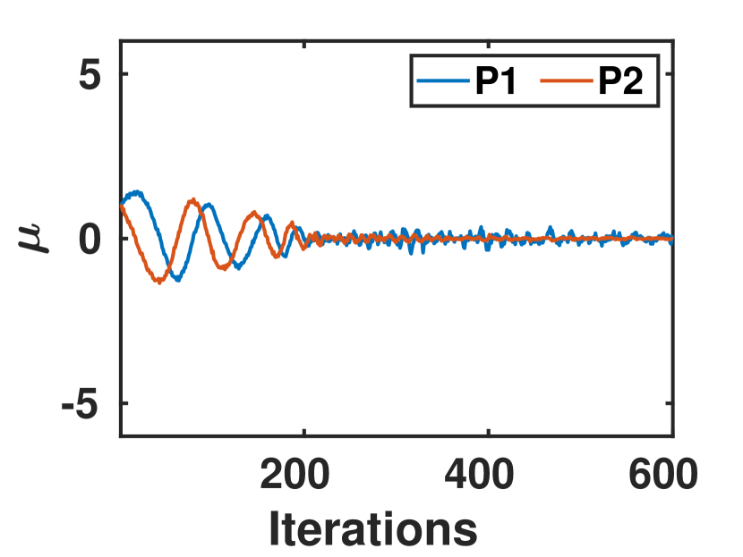
(b)

Figure 9: Policy trajectories of player 1 in a bilinear game. (a) TRGDA (b) TRCoPO

H.3 Matching pennies

The matching pennies game is played between two players, each player holds a coin and hence has two possible actions {Head, Tail}. Both the players secretly turn their coin to either head or tail. If the pennies of both the players matches then player 1 wins and player 2 looses. Otherwise, if pennies do not match then player 2 wins and player 1 loses. The game matrix is given in Tab. 3 captures win and lose of players for every possible action pair.

	H	T
H	1,-1	-1,1
T	-1,1	1,-1

Table 3: Game matrix for matching pennies game

Players’ policy is modeled with a two-class categorical distribution, which is randomly initialized. They sample actions from a softmax probability function over the categorical distribution and receive rewards for their actions according to the game matrix. We collect a batch of 1000 trajectories, to estimate gradient and bilinear terms in every epoch. CoPG converges to the Nash equilibrium of the game $(H,T)$ = $\bigl{(}\frac{1}{2},\frac{1}{2}\bigr{)}$. The experiment was performed for learning rates between 0.5 and 0.05 for 8 random seeds. The main paper features plot of CoPG vs GDA, but even for trust region approach we observe a similar contrast between TRCoPO and TRGDA. Starting from random policy initialization, TRCoPO converges to the unique Nash equilibrium of the game $(H,T)$ = $\bigl{(}\frac{1}{2},\frac{1}{2}\bigr{)}$, whereas TRGDA diverges for all KL-divergence bounds $\delta$. Fig. 10 shows this behaviour for a $\delta$ of 0.01. This experiment was performed also performed for 8 different random seeds and the results where consistent.

(a) TRGDA

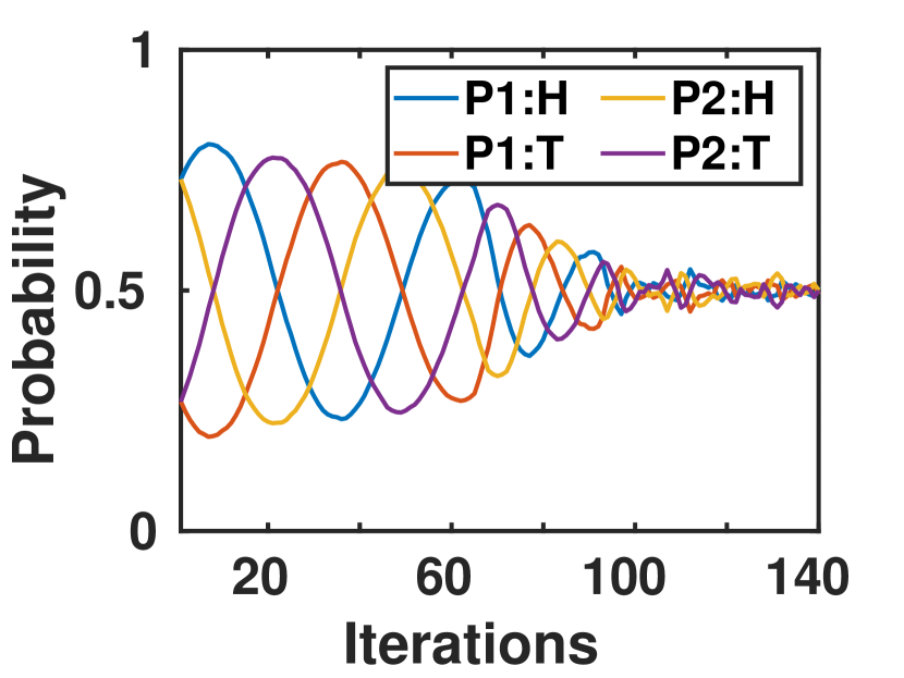
(b) TRCoPO

Figure 10: Policy trajectory in matching pennies game

H.4 Rock paper scissors

The rock paper scissors game is played between two players, each player has three possible actions {Rock, Paper, Scissors}. Both players will simultaneously display one of three actions: a rock, a paper, or a scissors. Rock beats scissors, scissors beat paper by cutting it, and paper beats rock by covering it. This is captured in the game matrix given by Tab. 4.

	Rock	Paper	Scissors
Rock	0,0	-1,1	1,-1
Paper	1,-1	0,0	-1,1
Scissors	-1,1	1,-1	0,0

Table 4: Game matrix for rock paper scissors game

Players’ policies are modeled with 3 class categorical distribution which is randomly initialized. Players sample action from a softmax probability function over categorical distribution. They receive a reward for their actions according to the game matrix. We collect a batch of 1000 trajectories. CoPG converges to the unique Nash equilibrium of the game, where probability of playing $(R,P,S)=(\frac{1}{3},\frac{1}{3},\frac{1}{3})$. The experiment was performed for learning rates between 0.5 and 0.05 for 8 random seeds where CoPG converged in all cases and GDA diverged. Similarly for the trust region approach, the TRCoPO agent converges to a unique Nash equilibrium of the game $(R,P,S)$= $\bigl{(}\frac{1}{3},\frac{1}{3},\frac{1}{3}\bigr{)}$, where as TRGDA diverges. Fig. 11 shows this behavior for $\delta$ of 0.001. The experiment was performed for 8 different random seeds.

(a) Player 1 TRGDA

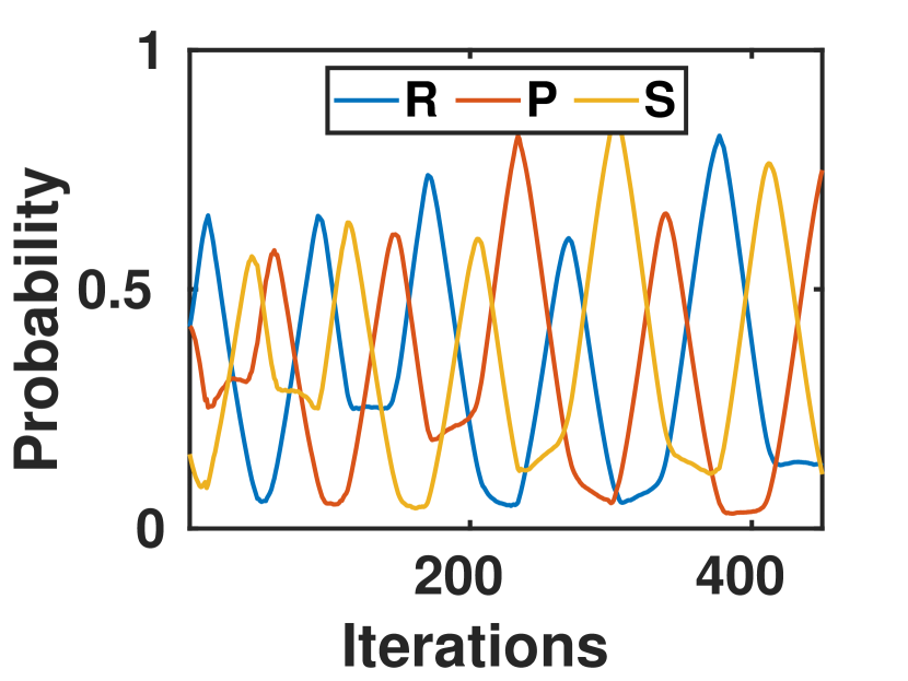
(b) Player 2 TRGDA

(c) Player 1 TRCoPO

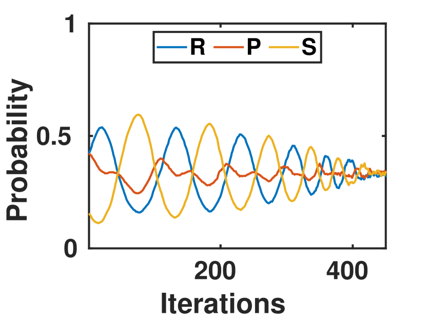
(d) Player 2 TRCoPO

Figure 11: Policy trajectory in a rock paper scissors game

H.5 Markov Soccer Game

The soccer game setup is shown in Fig. 4. It is played between two players A and B, both are randomly initialized in one of the 4x5 grid cells. The ball is also randomly initialised in one of the 4x5 grid cells, this contrast to the previous studies, where one of the players was randomly initialised with the ball. Players are supposed to pick up the ball and place it in the opponent’s goal. The players are allowed to move up, down, left, right or stand still. The player without the ball seizes the ball, if both players move simultaneously to the same grid cell. The game ends if a player scores a goal or none of them scores within 1000 steps. The winner receives a +1 reward and -1 is awarded to the losing player, hence the game is formulated as a zero sum game. This game does not have an optimal deterministic policy. This game depicts heavy interactions, where strategy depends on what the other player plays. Potentially, a good player can learn defending, dodging and scoring.

The state vector of a player P with respect to opponent O is $s^{P}=[x_{G_{O}},y_{G_{O}},x_{ball},y_{ball},x_{O},y_{O}]$, where $P,O\in\{A,B\}$. $G_{O}$ is goal of the opponent, $x,y$ refers to the relative position from the player to the subscript, e.g., $x_{O},y_{O}$ is the relative position to the opponent $O$. The state vector of the game used during training is $s=[s^{A},s^{B}]$, $s\in\mathcal{R}^{12}$, it captures the position of each player relative to the goal, the ball and relative to the opponent. The players’ policy maps state vector of the game to a categorical distribution with 5 categories using a network with two hidden layers one with 64 and other with 32 neurons. Players sample actions from a softmax probability function over the categorical distribution. The players were trained using GDA and CoPG. In both the algorithms, players were trained for roughly 30,000 episodes until the number of wins against any good player saturates. In each epoch we collected a batch which consists of 10 trajectories. All the parameters were the same throughout the training for CoPG and GDA. The experiment was tested with 6 different random seeds. We used learning rate of 0.01 and GAE for advantage estimation with $\lambda$ of 0.95 and $\gamma$ of 0.99.

Similarly, for the trust region approach the same game setting was used, with a maximum KL divergence $\delta$ of 0.0001. The players were trained with TRCoPO or TRGDA. Both the agents were trained for 5,000 episodes, each episode denotes a batch update where each batch consists of 10 trajectories. For comparison, we played 10000 games between agents trained using TRCoPO and with that using TRGDA, in which for 50% of the games TRCoPO was player A and for remaining TRGDA was player A. TRGDA generates unequal players, on competing with the stronger TRGDA agent, the TRCoPO agent still won more than 80% games against TRGDA as shown in Fig. 3(h). TRCoPO was able to learn better tactics for snatching the ball and dodging and defending its goal post. The histogram in Fig. 12, depicts a comparison of GDA, CoPG, TRGDA, and TRCoPO in the soccer game playing against each other.

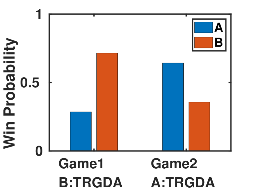
(a) GDA vs TRGDA

(b) TRGDA vs CoPG

(c) CoPG vs TRCoPO

(d) GDA vs TRCoPO

Figure 12: Win probability in soccer game played between GDA, CoPG, TRGDA and TRCoPO

H.6 The Car Racing game

Our final experimental setup is a racing game between two miniature race cars, where the goal is to finish the one lap race first. This involves both, learning a policy that can control a car at the limit of handling, as well as strategic interactions with the opposing car. Only if a player has the correct relative position to the opponent, this player is able to overtake or to block an overtaking. Our simulation study mimics the experimental platform located at ETH Zurich, which use miniature autonomous race cars.Following  [Liniger et al., 2015] the dynamics of one car is modeled as a dynamic bicycle model with Pacejka tire models  [Bakker et al., 1987]. However, compared to  [Liniger et al., 2015] we formulate the dynamics in curvilinear coordinates Vázquez et al. [2020] where the position and orientation are represented relative to a reference path. This change in coordinates significantly simplifies the definition of our reward, and simplified the policy learning. The resulting state of a single car is given as $z=[\rho,d,\mu,V_{x},V_{y},\psi]^{T}$, where $\rho$ is the progress along a reference path, $d$ is the deviation from a reference path, $\mu$ is the local heading with respect to the reference path, $V_{x}$ and $V_{y}$ are the longitudinal and the lateral velocity respectively in car frame and $\psi$ is the yawrate of the car. The inputs to the car is $[D,\delta]^{T}$, where $D\in[-1,1]$ is duty cycle input to the electric motor varying from full braking at $-1$ to full acceleration at $1$ and $\delta\in[-1,1]$ is the steering angle. The test track which consists of 13 turns with different curvature can be seen in Figure 13. For the reference path we used the X-Y path obtained by a laptime optimization tool Vázquez et al. [2020], note that it is not necessary to use a pre-optimize reference path, but we saw that it helped the convergence of the algorithm. Finally, to get a discrete time MDP we discretize the continuous time dynamics using an RK4 integrator with a sampling time of 0.03s.

Figure 13: Overtaking maneuvers of CoPG agents in the Car Racing Game. The thick line shows trajectory when the trailing agent overtook.

To formulate the racing game between two cars, we first define the state of the game as the concatenated state of the two players, $s=[z^{1},z^{2}]$. Second we convert the objective of finishing the race first without an accident into a zero sum game. Therefore, we define the following reward function using reward shaping. First to model our no accident constraints we use a freezing mechanism: (i) If the car is leaving the track we freeze it until the episode ends, (ii) if the cars collide, the rear car (car with the lower progress $\rho$) is stopped for 0.1s, which corresponds to a penalty of about two car lengths. Note that this gives an advantage to the car ahead, but in car racing the following car has to avoid collisions. Furthermore, an episode ends if both cars are either frozen due to leaving the track or the first car finished the lap. Finally, to reward the players receive at every time step is $r(s_{k},a^{1}_{k+1},a^{2}_{k+1})=\Delta\rho_{car_{1}}-\Delta\rho_{car_{2}}$, where $\Delta\rho=\rho_{k+1}-\rho_{k}$. This reward encourages the player to get as far ahead of the of the opponent player as possible. Note that the reward is zero sum, and the collision constraints do only indirectly influence the reward.

For the training we started the players on the start finish line ($\rho=0$) and randomly assigned $d\in\{0.1,-0.1\}$. We also limited one episode to 700 time steps, which is about twice as long as it takes an expert player to finish a lap. For each policy gradient step we generated a batch of 8 game trajectories, and we run the training for roughly 20000 epochs until the player consistently finish the lap. This takes roughly 62 hours of training for a single core CPU. To increase the performance and robustness of learning we adapted the learning rate with RMS prop for both GDA and CoPG and used a slow learning rate of $5.10^{-5}$ for both players. For our experiments we run 8 different random seeds and report the numbers of the best seed. As a policy we use a multi-layer perceptron with two hidden layers, each with 128 neurons, we used ReLU activation functions and a Tanh output layer to enforce the input constraints. GAE  is used for advantage estimation with $\lambda$ of $0.95$ and $\gamma$ of $0.99$. The same setting was also used to compare performance of TRCoPO and TRGDA. The maximum KL divergence $\delta$ was set between 1e-4 to 1e-5 and the training was performed for 8 different random seeds. The statistics of the experiments are presented in the main part of the paper Sec. 4.

H.7 Comparison with MADDPG and LOLA

Finally, we give more details on our comparison of CoPG with MADDPG and LOLA. We performed this comparison on the Markov soccer and the racing game. We start with the comparison for the Markov soccer game. To compare the performance of MADDPG on discrete action spaces (such as in the Markov soccer game), we used policies that can produce differentiable samples through a Gumbel-Softmax distribution, similar to  [Iqbal and Sha, 2019]. The rest of the experimental setup was kept as similar as explained in H.5, and we trained both MADDPG and CoPG. Fig. 14(a) shows that a policy learned by MADDPG performs similar to that of GDA. But when the MADDPG player competes against CoPG, the CoPG agent wins 80% of the games. Second we studied LOLA, we observed that LOLA learns better policies than GDA potentially due to the second level reasoning, but LOLA still loses 72% of the games when playing against CoPG. Fig. 14 show the number of games won by CoPG when competing against MADDPG and LOLA.

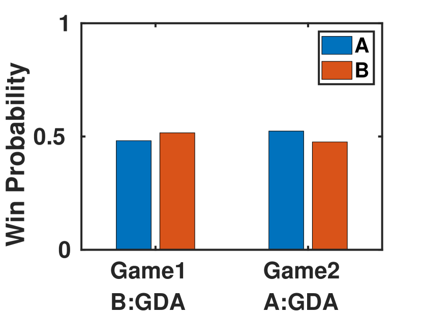
(a) GDA vs MADDPG

(b) CoPG vs MADDPG

(c) LOLA vs GDA

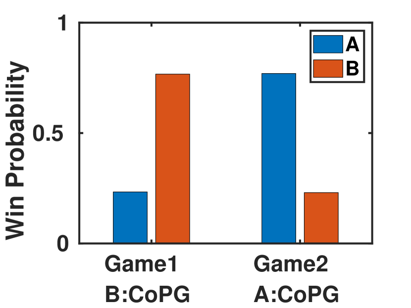
(d) CoPG vs LOLA

Figure 14: Comparison with LOLA and MADDPG on the Markov soccer game

Next we evaluated MADDPG and LOLA in the game of Car Racing, where we kept all the setting identical to H.6. Fig. 5(e) show the progress of an MADDPG agent during learning, and we can see that it performs similar to GDA. The car learns to drive up to 30% of the track, but after that the agents show oscillatory behaviour in training. We also performed this experiment with LOLA, but due to the variance in estimating the bilinear term and more importantly the non adaptive learning rate of LOLA it does not learn to drive around the track.

References

- Aleksandrov et al. (1968) V. M. Aleksandrov, V. I. Sysoyev, and V. V. Shemeneva. Stochastic optimization. Engineering Cybernetics, 5(11-16):229–256, 1968.
- Azizzadenesheli et al. (2020) Kamyar Azizzadenesheli, Yisong Yue, and Anima Anandkumar. Policy gradient in partially observable environments: Approximation and convergence. arXiv preprint arXiv:1810.07900, 2020.
- Baird (1993) Leemon C Baird, III. Advantage updating. WRIGHT LAB WRIGHT-PATTERSON AFB OH, 1993. URL https://apps.dtic.mil/dtic/tr/fulltext/u2/a280862.pdf.
- Bakker et al. (1987) Egbert Bakker, Lars Nyborg, and Hans B. Pacejka. Tyre modelling for use in vehicle dynamics studies. In SAE Technical Paper. SAE International, 02 1987. doi: 10.4271/870421. URL https://doi.org/10.4271/870421.
- Balduzzi et al. (2018) David Balduzzi, Sébastien Racanière, James Martens, Jakob N. Foerster, Karl Tuyls, and Thore Graepel. The mechanics of n-player differentiable games. CoRR, abs/1802.05642, 2018. URL http://arxiv.org/abs/1802.05642.
- Blum et al. (2008) Avrim Blum, MohammadTaghi Hajiaghayi, Katrina Ligett, and Aaron Roth. Regret minimization and the price of total anarchy. In Proceedings of the Fortieth Annual ACM Symposium on Theory of Computing, STOC ’08, page 373–382, New York, NY, USA, 2008. Association for Computing Machinery. ISBN 9781605580470. doi: 10.1145/1374376.1374430. URL https://doi.org/10.1145/1374376.1374430.
- Bowling et al. (2017) Michael Bowling, Neil Burch, Michael Johanson, and Oskari Tammelin. Heads-up limit hold’em poker is solved. Commun. ACM, 60(11):81–88, October 2017. ISSN 0001-0782. doi: 10.1145/3131284. URL https://doi.org/10.1145/3131284.
- Buşoniu and Babuška (2010) Lucian Buşoniu and Bart Babuška, Robertand De Schutter. Multi-agent Reinforcement Learning: An Overview, pages 183–221. Springer Berlin Heidelberg, Berlin, Heidelberg, 2010. ISBN 978-3-642-14435-6. doi: 10.1007/978-3-642-14435-6_7. URL https://doi.org/10.1007/978-3-642-14435-6_7.
- Cesa-Bianchi and Lugosi (2006) Nicolo Cesa-Bianchi and Gábor Lugosi. Prediction, learning, and games. Cambridge university press, 2006.
- Dantzig (1998) George Bernard Dantzig. Linear programming and extensions, volume 48. Princeton university press, 1998.
- Daskalakis et al. (2017) Constantinos Daskalakis, Andrew Ilyas, Vasilis Syrgkanis, and Haoyang Zeng. Training gans with optimism. CoRR, abs/1711.00141, 2017. URL http://arxiv.org/abs/1711.00141.
- Filar and Vrieze (2012) Jerzy Filar and Koos Vrieze. Competitive Markov decision processes. Springer Science & Business Media, 2012.
- Foerster et al. (2017a) Jakob N. Foerster, Richard Y. Chen, Maruan Al-Shedivat, Shimon Whiteson, Pieter Abbeel, and Igor Mordatch. Learning with opponent-learning awareness. CoRR, abs/1709.04326, 2017a. URL http://arxiv.org/abs/1709.04326.
- Foerster et al. (2017b) Jakob N. Foerster, Gregory Farquhar, Triantafyllos Afouras, Nantas Nardelli, and Shimon Whiteson. Counterfactual multi-agent policy gradients. CoRR, abs/1705.08926, 2017b. URL http://arxiv.org/abs/1705.08926.
- Frénay and Saerens (2009) Benoít Frénay and Marco Saerens. Ql2, a simple reinforcement learning scheme for two-player zero-sum markov games. Neurocomput., 72(7–9):1494–1507, March 2009. ISSN 0925-2312. doi: 10.1016/j.neucom.2008.12.022. URL https://doi.org/10.1016/j.neucom.2008.12.022.
- Gemp and Mahadevan (2018) Ian Gemp and Sridhar Mahadevan. Global convergence to the equilibrium of gans using variational inequalities. CoRR, abs/1808.01531, 2018. URL http://arxiv.org/abs/1808.01531.
- Gidel et al. (2018) Gauthier Gidel, Reyhane Askari Hemmat, Mohammad Pezeshki, Gabriel Huang, Rémi Le Priol, Simon Lacoste-Julien, and Ioannis Mitliagkas. Negative momentum for improved game dynamics. CoRR, abs/1807.04740, 2018. URL http://arxiv.org/abs/1807.04740.
- Gilpin et al. (2007) Andrew Gilpin, Samid Hoda, Javier Peña, and Tuomas Sandholm. Gradient-based algorithms for finding nash equilibria in extensive form games. In WINE, 2007.
- Goodfellow et al. (2014) Ian Goodfellow, Jean Pouget-Abadie, Mehdi Mirza, Bing Xu, David Warde-Farley, Sherjil Ozair, Aaron Courville, and Yoshua Bengio. Generative adversarial nets. In Advances in neural information processing systems, pages 2672–2680, 2014.
- Grau-Moya et al. (2018) Jordi Grau-Moya, Felix Leibfried, and Haitham Bou-Ammar. Balancing two-player stochastic games with soft q-learning. In Proceedings of the 27th International Joint Conference on Artificial Intelligence, IJCAI’18, page 268–274. AAAI Press, 2018. ISBN 9780999241127.
- Greenwald and Hall (2003) Amy Greenwald and Keith Hall. Correlated-q learning. In Proceedings of the Twentieth International Conference on International Conference on Machine Learning, ICML’03, page 242–249. AAAI Press, 2003. ISBN 1577351894.
- Hartline et al. (2015) Jason Hartline, Vasilis Syrgkanis, and Éva Tardos. No-regret learning in bayesian games. In Proceedings of the 28th International Conference on Neural Information Processing Systems - Volume 2, NIPS’15, page 3061–3069, Cambridge, MA, USA, 2015. MIT Press.
- He et al. (2016) He He, Jordan L. Boyd-Graber, Kevin Kwok, and Hal Daumé III. Opponent modeling in deep reinforcement learning. CoRR, abs/1609.05559, 2016. URL http://arxiv.org/abs/1609.05559.
- Heinrich and Silver (2016) Johannes Heinrich and David Silver. Deep reinforcement learning from self-play in imperfect-information games. CoRR, abs/1603.01121, 2016. URL http://arxiv.org/abs/1603.01121.
- Heinrich et al. (2015) Johannes Heinrich, Marc Lanctot, and David Silver. Fictitious self-play in extensive-form games. In Proceedings of the 32nd International Conference on International Conference on Machine Learning - Volume 37, ICML’15, page 805–813. JMLR.org, 2015.
- Hernandez-Leal et al. (2019) Pablo Hernandez-Leal, Bilal Kartal, and Matthew E. Taylor. A survey and critique of multiagent deep reinforcement learning. Autonomous Agents and Multi-Agent Systems, 33(6):750–797, Oct 2019. ISSN 1573-7454. doi: 10.1007/s10458-019-09421-1. URL http://dx.doi.org/10.1007/s10458-019-09421-1.
- Hu and Wellman (2003) Junling Hu and Michael P. Wellman. Nash q-learning for general-sum stochastic games. J. Mach. Learn. Res., 4(null):1039–1069, December 2003. ISSN 1532-4435.
- Iqbal and Sha (2019) Shariq Iqbal and Fei Sha. Actor-attention-critic for multi-agent reinforcement learning. In Kamalika Chaudhuri and Ruslan Salakhutdinov, editors, Proceedings of the 36th International Conference on Machine Learning, volume 97 of Proceedings of Machine Learning Research, pages 2961–2970, Long Beach, California, USA, 09–15 Jun 2019. PMLR. URL http://proceedings.mlr.press/v97/iqbal19a.html.
- Kakade and Langford (2002) Sham Kakade and John Langford. Approximately optimal approximate reinforcement learning. In ICML, volume 2, pages 267–274, 2002.
- Kakade (2002) Sham M Kakade. A natural policy gradient. In Advances in neural information processing systems, pages 1531–1538, 2002.
- Koller et al. (1995) Daphne Koller, Nimrod Megiddo, and Bernhard von Stengel. Efficient computation of equilibria for extensive two-person games. Games and Economic Behavior, 14, 10 1995. doi: 10.1006/game.1996.0051.
- Leibo et al. (2017) Joel Z. Leibo, Vinícius Flores Zambaldi, Marc Lanctot, Janusz Marecki, and Thore Graepel. Multi-agent reinforcement learning in sequential social dilemmas. CoRR, abs/1702.03037, 2017. URL http://arxiv.org/abs/1702.03037.
- Liniger and Lygeros (2020) Alexander Liniger and John Lygeros. A noncooperative game approach to autonomous racing. IEEE Transactions on Control Systems Technology, 28(3):884–897, 2020.
- Liniger et al. (2015) Alexander Liniger, Alexander Domahidi, and Manfred Morari. Optimization-based autonomous racing of 1: 43 scale rc cars. Optimal Control Applications and Methods, 36(5):628–647, 2015.
- Littman (1994) M. L. Littman. Markov games as a framework for multi-agent reinforcement learning, 1994.
- Littman (2001a) Michael Littman. Value-function reinforcement learning in markov games. Cognitive Systems Research, 2:55–66, 04 2001a. doi: 10.1016/S1389-0417(01)00015-8.
- Littman (2001b) Michael L. Littman. Friend-or-foe q-learning in general-sum games. In Proceedings of the Eighteenth International Conference on Machine Learning, ICML ’01, page 322–328, San Francisco, CA, USA, 2001b. Morgan Kaufmann Publishers Inc. ISBN 1558607781.
- Lowe et al. (2017) Ryan Lowe, Yi Wu, Aviv Tamar, Jean Harb, Pieter Abbeel, and Igor Mordatch. Multi-agent actor-critic for mixed cooperative-competitive environments. Neural Information Processing Systems (NIPS), 2017.
- Matignon et al. (2012) Laetitia Matignon, Guillaume J. Laurent, and Nadine Le Fort-Piat. Independent reinforcement learners in cooperative markov games: a survey regarding coordination problems. The Knowledge Engineering Review, 27(1):1–31, 2012. doi: 10.1017/S0269888912000057.
- Mazumdar et al. (2019) Eric Mazumdar, Lillian J. Ratliff, Michael I. Jordan, and S. Shankar Sastry. Policy-gradient algorithms have no guarantees of convergence in linear quadratic games, 2019.
- Mertikopoulos et al. (2018a) Panayotis Mertikopoulos, Christos Papadimitriou, and Georgios Piliouras. Cycles in adversarial regularized learning. In Proceedings of the Twenty-Ninth Annual ACM-SIAM Symposium on Discrete Algorithms, pages 2703–2717. SIAM, 2018a.
- Mertikopoulos et al. (2018b) Panayotis Mertikopoulos, Houssam Zenati, Bruno Lecouat, Chuan-Sheng Foo, Vijay Chandrasekhar, and Georgios Piliouras. Mirror descent in saddle-point problems: Going the extra (gradient) mile. CoRR, abs/1807.02629, 2018b. URL http://arxiv.org/abs/1807.02629.
- Mescheder et al. (2017) Lars M. Mescheder, Sebastian Nowozin, and Andreas Geiger. The numerics of gans. CoRR, abs/1705.10461, 2017. URL http://arxiv.org/abs/1705.10461.
- Moravcík et al. (2017) Matej Moravcík, Martin Schmid, Neil Burch, Viliam Lisý, Dustin Morrill, Nolan Bard, Trevor Davis, Kevin Waugh, Michael Johanson, and Michael H. Bowling. Deepstack: Expert-level artificial intelligence in no-limit poker. CoRR, abs/1701.01724, 2017. URL http://arxiv.org/abs/1701.01724.
- Neller and Lanctot (2013) Todd W. Neller and Marc Lanctot. An introduction to counterfactual regret minimization. The Fourth Symposium on Educational Advances in Artificial Intelligence (EAAI-2013), 2013, 2013. URL http://modelai.gettysburg.edu/2013/cfr/cfr.pdf.
- Paszke et al. (2019) Adam Paszke, Sam Gross, Francisco Massa, Adam Lerer, James Bradbury, Gregory Chanan, Trevor Killeen, Zeming Lin, Natalia Gimelshein, Luca Antiga, Alban Desmaison, Andreas Kopf, Edward Yang, Zachary DeVito, Martin Raison, Alykhan Tejani, Sasank Chilamkurthy, Benoit Steiner, Lu Fang, Junjie Bai, and Soumith Chintala. Pytorch: An imperative style, high-performance deep learning library. In Advances in Neural Information Processing Systems 32. Curran Associates, Inc., 2019. URL http://papers.neurips.cc/paper/9015-pytorch-an-imperative-style-high-performance-deep-learning-library.pdf.
- Pérolat et al. (2018) Julien Pérolat, Bilal Piot, and Olivier Pietquin. Actor-critic fictitious play in simultaneous move multistage games. In Amos J. Storkey and Fernando Pérez-Cruz, editors, International Conference on Artificial Intelligence and Statistics, AISTATS 2018, 9-11 April 2018, Playa Blanca, Lanzarote, Canary Islands, Spain, volume 84 of Proceedings of Machine Learning Research, pages 919–928. PMLR, 2018. URL http://proceedings.mlr.press/v84/perolat18a.html.
- Puterman (2014) Martin L Puterman. Markov decision processes: discrete stochastic dynamic programming. John Wiley & Sons, 2014.
- Raghu et al. (2017) Maithra Raghu, Alex Irpan, Jacob Andreas, Robert Kleinberg, Quoc V. Le, and Jon M. Kleinberg. Can deep reinforcement learning solve erdos-selfridge-spencer games? CoRR, abs/1711.02301, 2017. URL http://arxiv.org/abs/1711.02301.
- Raileanu et al. (2018) Roberta Raileanu, Emily Denton, Arthur Szlam, and Rob Fergus. Modeling others using oneself in multi-agent reinforcement learning. CoRR, abs/1802.09640, 2018. URL http://arxiv.org/abs/1802.09640.
- Robbins and Monro (1951) Herbert Robbins and Sutton Monro. A stochastic approximation method. The annals of mathematical statistics, pages 400–407, 1951.
- Roughgarden (2010) Tim Roughgarden. Algorithmic game theory. Communications of the ACM, 53(7):78–86, 2010.
- Schulman et al. (2015) John Schulman, Sergey Levine, Philipp Moritz, Michael I. Jordan, and Pieter Abbeel. Trust region policy optimization, 2015.
- Schulman et al. (2016) John Schulman, Philipp Moritz, Sergey Levine, Michael I. Jordan, and Pieter Abbeel. High-dimensional continuous control using generalized advantage estimation. In Yoshua Bengio and Yann LeCun, editors, 4th International Conference on Learning Representations, ICLR 2016, San Juan, Puerto Rico, May 2-4, 2016, Conference Track Proceedings, 2016. URL http://arxiv.org/abs/1506.02438.
- Schäfer and Anandkumar (2019) Florian Schäfer and Anima Anandkumar. Competitive gradient descent, 2019.
- Schäfer et al. (2019) Florian Schäfer, Hongkai Zheng, and Anima Anandkumar. Implicit competitive regularization in gans, 2019.
- Shalev-shwartz and Singer (2007) Shai Shalev-shwartz and Yoram Singer. Convex repeated games and fenchel duality. In B. Schölkopf, J. C. Platt, and T. Hoffman, editors, Advances in Neural Information Processing Systems 19, pages 1265–1272. MIT Press, 2007. URL http://papers.nips.cc/paper/3107-convex-repeated-games-and-fenchel-duality.pdf.
- Shewchuk (1994) Jonathan R Shewchuk. An introduction to the conjugate gradient method without the agonizing pain. Technical report, Carnegie Mellon University, USA, 1994.
- Silver et al. (2016) David Silver, Aja Huang, Chris J Maddison, Arthur Guez, Laurent Sifre, George Van Den Driessche, Julian Schrittwieser, Ioannis Antonoglou, Veda Panneershelvam, Marc Lanctot, et al. Mastering the game of go with deep neural networks and tree search. nature, 529(7587):484, 2016.
- Srinivasan et al. (2018) Sriram Srinivasan, Marc Lanctot, Vinícius Flores Zambaldi, Julien Pérolat, Karl Tuyls, Rémi Munos, and Michael Bowling. Actor-critic policy optimization in partially observable multiagent environments. CoRR, abs/1810.09026, 2018. URL http://arxiv.org/abs/1810.09026.
- Sutton and Barto (2018) Richard S Sutton and Andrew G Barto. Reinforcement learning: An introduction. MIT press, 2018.
- Sutton et al. (2000) Richard S Sutton, David A McAllester, Satinder P Singh, and Yishay Mansour. Policy gradient methods for reinforcement learning with function approximation. In Advances in neural information processing systems, pages 1057–1063, 2000.
- Tampuu et al. (2015) Ardi Tampuu, Tambet Matiisen, Dorian Kodelja, Ilya Kuzovkin, Kristjan Korjus, Juhan Aru, Jaan Aru, and Raul Vicente. Multiagent cooperation and competition with deep reinforcement learning, 2015.
- Tesauro (1995) Gerald Tesauro. Temporal difference learning and td-gammon. Communications of the ACM, 38(3):58–68, 1995.
- Vázquez et al. (2020) Jose L. Vázquez, Marius Brühlmeier, Alexander Liniger, Alisa Rupenyan, and John Lygeros. Optimization-based hierarchical motion planning for autonomous racing. ArXiv, abs/2003.04882, 2020.
- Wald (1945) Abraham Wald. Sequential tests of statistical hypotheses. The annals of mathematical statistics, 16(2):117–186, 1945.
- Yazıcı et al. (2018) Yasin Yazıcı, Chuan-Sheng Foo, Stefan Winkler, Kim-Hui Yap, Georgios Piliouras, and Vijay Chandrasekhar. The unusual effectiveness of averaging in gan training, 2018.
- Zhang et al. (2019) Kaiqing Zhang, Zhuoran Yang, and Tamer Başar. Policy optimization provably converges to nash equilibria in zero-sum linear quadratic games, 2019.
- Zhou et al. (1996) Kemin Zhou, John Comstock Doyle, Keith Glover, et al. Robust and optimal control, volume 40. Prentice hall New Jersey, 1996.
- Zinkevich et al. (2008) Martin Zinkevich, Michael Johanson, Michael Bowling, and Carmelo Piccione. Regret minimization in games with incomplete information. In J. C. Platt, D. Koller, Y. Singer, and S. T. Roweis, editors, Advances in Neural Information Processing Systems 20, pages 1729–1736. Curran Associates, Inc., 2008. URL http://papers.nips.cc/paper/3306-regret-minimization-in-games-with-incomplete-information.pdf.