Black Rubber and the Non-linear
Elastic Response of Scale Invariant Solids

Abstract

We discuss the nonlinear elastic response in scale invariant solids. Following previous work, we split the analysis into two basic options: according to whether scale invariance (SI) is a manifest or a spontaneously broken symmetry. In the latter case, one can employ effective field theory methods, whereas in the former we use holographic methods. We focus on a simple class of holographic models that exhibit elastic behaviour, and obtain their nonlinear stress-strain curves as well as an estimate of the elasticity bounds — the maximum possible deformation in the elastic (reversible) regime. The bounds differ substantially in the manifest or spontaneously broken SI cases, even when the same stress-strain curve is assumed in both cases. Additionally, the hyper-elastic subset of models (that allow for large deformations) is found to have stress-strain curves akin to natural rubber. The holographic instances in this category, which we dub black rubber, display richer stress-strain curves – with two different power-law regimes at different magnitudes of the strain.

1 Introduction

The response of materials under mechanical (or elastic) deformations is a basic aspect of matter, which is important to understand and characterize. This is an old field of study because of the many practical applications and a large part of it is well understood since long ago landau7 ; Lubensky .

The response is best understood when restricted to the ‘linear’ regime (small deformations), but there are many examples of solids that can undertake large deformations Ogden2004 . Common examples of these are the rubbers, but more generically they are referred to as hyper-elastic materials. The non-linear response that these materials exhibit is encoded in the stress-strain relations – the amount of constant stress that must be applied in order to deform by a certain amount the material – see Fig. 1 for a prototypical example. These curves can be easily obtained from experiments, but they are usually difficult to compute from the microscopic ingredients (even within the reversible regime, that is neglecting plasticity and dissipative effects), especially so in strongly coupled materials. Moreover, the nonlinear response is characterized by a rather large number of parameters/observables (e.g., all the derivatives of the stress-strain curve at the origin, the maximum strain that the material can undertake, etc), and it might well be that there exist correlations between them. This motivates the study of the nonlinear mechanical response using effective low energy methods, which on their own might capture some of these correlations and even how these parameters depend on external parameters (temperature, etc).

The ‘continuum limit’ description of mechanical deformations represents one such effective method that is useful for nonlinear response. This approach embodies already a broad literature, see ZAMM:ZAMM19850650903 for a review. As in hydrodynamics, the medium is described by a 3-vector $\pi_{i}(t,x^{j})$, the displacement vector of the solid elements. How the material deforms is encoded in its gradient, the so-called strain tensor $\epsilon_{ij}\sim\partial_{(i}\pi_{j)}$. The main difference between solids and fluids in this language is that a solid responds to a constant external stress $\sigma_{ij}$ with constant $\epsilon_{ij}$, whereas a viscous fluid responds with a constant strain rate, $\dot{\epsilon}_{ij}$. The punchline, though, is that the same kind of effective description is possible both for fluids and solids at small frequencies (and momenta) PhysRevA.6.2401 .

For small applied stresses the response is linear, $\sigma_{ij}\propto\epsilon_{ij}$, and the proportionality constants are usually called elastic moduli. Nonlinear elasticity concerns the relation between the stress and strain tensors beyond the linear approximation. The mathematical formalism required for this in the continuum limit was developed long ago, see ZAMM:ZAMM19850650903 for a comprehensive review. This results especially relevant for hyper-elastic materials or elastomers, which allow for large reversible deformations. For them, the continuum limit description takes the form of a nonlinear theory for the displacement vector field $\pi_{i}$ that can be specified by an energy function (how the energy density depends on $\epsilon_{ij}$) or a (nonlinear) constitutive relation.

Figure 1: Cartoon of a typical stress-strain curve of a hyper-elastic material enlighten70333 . In light blue shade the linear regime, in which stress $\propto$ strain. At large strain deformation, the stress-strain relation can display a power law behaviour, $\sigma\propto\epsilon^{\nu}$, with some exponent $\nu$. The light red area illustrates this behaviour with $\nu>1$. Materials typically break or fracture after some critical deformation, which translates in the stress-train curves terminating at some point. The red star indicates the breaking point.

Symmetries allow to translate nonlinear elasticity into quantum field theory language. Given that condensed matter breaks spontaneously spacetime translations and boosts, it is possible to catch the dynamics for the lightest degrees of freedom using the methods of Effective Field Theory (EFT) applied to the spontaneous breaking of these symmetries. In solids, the Goldstone bosons associated to this spontaneous breaking can be identified as the (‘acoustic’) phonons Leutwyler:1996er ; Dubovsky:2011sj . These phonons are the fluctuations in the displacement vector $\pi_{i}$, they are indeed gapless and therefore belong to the lowest lying excitations, which makes the whole EFT construction consistent.

The possible form of the full nonlinear effective Lagrangian for the phonon fields can be obtained using the coset construction applied to spacetime symmetries, see Nicolis:2013lma ; Nicolis:2015sra . It was recognized in Alberte:2018doe that, for solids, the resulting phonon effective Lagrangian takes precisely the same form as the continuum limit nonlinear elasticity theory for the displacement vector $\pi^{i}(t,x^{j})$ for hyper-elastic materials ZAMM:ZAMM19850650903 (at leading order in derivatives). The crucial advantage is that the solid EFTs are full-fledged effective Lagrangians that include dynamical effects and relativistic corrections among other improvements Alberte:2018doe .

Let us emphasize that, even if they are not formulated in terms of the microscopic degrees of freedom, the EFT methods have stringent predictive and constraining power. This point was illustrated in Alberte:2018doe , where the correlation between various nonlinear observables was made manifest in the form of elasticity bounds – limits on the strain that a material of certain type can possibly withstand depending on other properties of the material. The simplest example arises by considering a class of materials characterized by power-law scaling in the stress-strain curve, schematically,

$$\sigma\sim\epsilon^{\nu}\,,$$ (1)

with some arbitrary exponent $\nu$. Some elastomers in nature follow such a power-law at large deformation ZAMM:ZAMM19850650903 with a variety of exponents. For a general analysis of the elastic response, one can treat $\nu$ simply as an effective parameter to describe the nonlinear response (at least in a class of materials). Interestingly, assuming this power-law response is enough to place a priori an upper limit on the maximum strain deformation, $\epsilon_{max}$, that the material can undertake Alberte:2018doe . This maximum deformation $\epsilon_{max}$ plays the role of (an upper limit to) the mechanical breaking or failure point of materials.

A nontrivial outcome of the EFT methods is that one can establish a relation between these two nonlinear elasticity parameter, $\nu$ and $\epsilon_{max}$. Let us emphasize two points in order to highlight the potential value of the EFT methodology for nonlinear elasticity. First, we stress that the correlation between $\nu$ and $\epsilon_{max}$ is entirely based on low energy EFT properties. This illustrates that it is possible to understand some of the properties of the nonlinear response just from the low energy theory, that is, independently from the microscopic details. Second, the constraining power of the EFT methods is expected to apply to many other nonlinear elasticity parameter, beyond the one examined in Ref. Alberte:2018doe . This is especially clear taking into account that the main benefit from the EFT methods is that the full nonlinear structure of the theory is fixed by the symmetries.

This encourages us to continue the analysis to other cases, in particular to the more sophisticated materials that exhibit scale invariance (SI). As elaborated in Baggioli:2019elg , this case deserves a special treatment, because SI can be realized in several ways and this affects the elastic response – even in the linear response regime. The main distinction concerns whether SI is a broken or a manifest symmetry of the low energy dynamics. The latter case implies that the theory that describes the solid excitations must be akin to a conformal field theory (CFT). In this case, bottom-up AdS/CFT methods Baggioli:2019rrs provide a useful tool to properly model the material. The opposite case – with SI as a spontaneously broken – can be treated instead within the more conventional EFT methods Leutwyler:1996er ; Dubovsky:2011sj ; Nicolis:2013lma ; Nicolis:2015sra .

The existence of these two types of SI solids gives a ‘bonus’ of motivation to the present study, as it is interesting to compare how much the low-energy constraints in the nonlinear response differ depending on whether SI is manifest or spontaneously broken. As we will see, there is a significant difference in the relation between the nonlinear parameters introduced above ($\nu$ and $\epsilon_{max}$) for the two types of SI materials.

A good fraction of this work is devoted to provide the tools to compute the nonlinear mechanical response for the manifest SI case, by exploiting holographic AdS/CFT methods. The main technical development that we present is the construction of a large family of asymptotically AdS black brane solutions that are subject to finite mechanical deformations and we obtain their stress-strain curves. We shall find that a certain class of models allows for black branes that can be deformed elastically by large amounts without breaking. In these cases, their stress-strain diagrams are similar to that of natural rubber (with $\mathcal{O}(1)$ values of the exponents $\nu$, see below), so isn’t a great stretch to call these solutions black rubber.

These solutions can be found semi-analytically in the simplest models, which include the displacement vectors $\pi^{i}$ as new explicit degrees of freedom – also called Stückelberg fields in the previous literature. This paper builds on the recent holographic massive gravity models Vegh:2013sk ; Blake:2013owa ; Andrade:2013gsa ; Baggioli:2014roa ; Alberte:2015isw ; Ammon:2020xyv which realize in a simple way the spontaneous breaking of translational invariance in ‘critical’ materials (with manifest SI at low energies).

More recently, several works have improved the framework to accommodate for the spontaneous breaking of translations Baggioli:2014roa and the study of the linear elastic response Alberte:2015isw , the vibrational modes of the systems Alberte:2017cch ; Alberte:2017oqx , their viscoelastic nature Alberte:2016xja ; Baggioli:2018bfa ; Andrade:2019zey ; Baggioli:2019mck and their hydrodynamic and physical description Ammon:2020xyv ; Baggioli:2020nay .

2 Nonlinear Elastic response

In this Section, we review the basic formalism to describe the elastic response under finite (“large”) deformations or applied stresses. Linear elasticity theory describes how materials deform in presence of a small (“infinitesimal”) external deformation. The mechanical deformation for a solid in $d+1$ dimensions can be described by a $d$-dimensional vector field, the displacement vector,

$$\pi_{i}(x)\,,$$ (2)

that measures the physical distance from equilibrium position at any given point in the solid. Out of the $\pi_{i}$, one builds a rank-2 symmetric tensor, called the strain tensor as

$$\epsilon_{ij}\,\equiv\,\partial_{i}\pi_{j}\,+\,\partial_{j}\,\pi_{i}~{}.$$ (3)

Volume-preserving deformations satisfy

$$\epsilon_{ii}=0$$ (4)

and are called shear strain. Similarly, strains that change volume but not shape satisfy

$$\epsilon_{ij}\propto\delta_{ij}$$ (5)

and they are called pure bulk deformations.

In most materials, at small enough deformations (small strains), there is a linear relation between the stress needed to apply on the material and the generated strain. Mathematically, this translates into a linear relation between $\epsilon_{ij}$ and the stress tensor $\sigma_{ij}$ of the form,

$$\sigma_{ij}\,=\,C_{ijkl}\,\epsilon_{kl}~{}.$$ (6)

The elastic tensor, $C_{ijkl}$, is well known to reduce to just two parameters for homogeneous and isotropic materials: the shear and bulk moduli, which encode the linear response to pure shear and pure bulk deformations respectively.

Non-linear elasticity concerns the relation between stress and strain beyond linear level – conceptually, the full functional form of $\sigma_{ij}=\sigma_{ij}\left(\epsilon_{kl}\right)$. In order to extend the relation to the non-linear regime, one must pay attention to how the strain deformations are defined nonlinearly.

Reviewing the logic, one realizes that in materials that are homogeneous and isotropic at long wavelengths there symmetry allows to choose what we call solid elements so that their equilibrium positions coincide with the ‘cartesian’ coordinates. This suggests to introduce another variable to describe the state of deformation,

$$\phi^{I}=\delta^{I}_{i}x^{i}+\pi^{I}\,,$$ (7)

so that equilibrium corresponds to ${\phi}^{I}_{\text{eq}}=\delta^{I}_{i}x^{i}$. This variable is also more amenable to treat homogeneity and isotropy as an internal symmetry for the scalar fields $\Phi^{I}$, as done in Leutwyler:1996er ; Dubovsky:2011sj , which is why the index label on $\pi^{I}$ has been capitalized.

A general state of deformation that is constant along the material is then given by

$$\phi^{I}=O^{I}_{j}\,x^{j}\;,$$ (8)

with an arbitrary constant matrix $O^{I}_{j}$, which is a useful way to parameterize the strain tensor for finite deformations. One can easily convince oneself that in the homogeneous and isotropic limit one can restrict $O^{I}_{j}$ to be a symmetric matrix with no loss of generality. Isotropy forbids the presence of any background shear strain.

The advantage of using (7) as a variable is now clear: the natural extension that supersedes (4) to the nonlinear regime is

$${\rm Det}\left(\,O^{I}_{j}\,\right)=1\;.$$ (9)

This condition extends to non-linear level the requirement that the deformation described by the matrix $O^{I}_{j}$ does not change the volume of the system.

For illustration, in $2+1$ dimensions, $O^{I}_{j}$ is simply a $2\times 2$ symmetric matrix, which contains only 3 free parameters. We shall stick to the following parametrization,

$$O^{I}_{j}\,=\,\alpha\begin{pmatrix}\sqrt{1+\varepsilon^{2}/4}&\varepsilon/2\\ \varepsilon/2&\sqrt{1+\varepsilon^{2}/4}\end{pmatrix}~{},$$ (10)

where $\varepsilon$ serves as a nonlinear version of the shear deformation and $\alpha$ for the pure bulk deformations. We are dropping the ‘third’ parameter, $\tilde{\varepsilon}$, for deformations of the form $O^{I}_{j}={\rm diag}(e^{\tilde{\varepsilon}},e^{-\tilde{\varepsilon}})$ because they only differ from $\varepsilon$ deformations in that the shear is introduced in a basis rotated by $45$ degrees. Since we are assuming homogeneous and isotropic materials, it suffices to consider one of the two shear ‘polarizations’.

The stress-strain curves can now be extracted by computing the stresses in the material that are necessary to support a configuration (8). Once the low energy theory for the material is specified, this reduces to just looking at the stresses produced by these configurations. Continuing in the $2+1$ example above, this can be done by computing the stress

$$\sigma_{ij}\equiv T_{ij}$$ (11)

as a function of the deformation $O^{I}_{j}$.

Materials that can be deformed by large amounts while in a reversible fashion are generically called hyper-elastic. For these, the stress-strain relation can be obtained from a so-called energy function scalar function enlighten70333 ,

$${\cal E}(O^{I}_{j})\,,$$ (12)

that characterizes how energetically ‘expensive’ every deformation is.

From now on, we will consider materials with this property and which realize scale invariance (SI), and we will distinguish between two sub-cases depending on how SI is realized:

• critical solids, that is, which realize SI as a manifest symmetry at low energies (Section 3);

• solids with spontaneously broken SI, with a gapped spectrum and thus have phonons as the lowest-energy excitations (Section 4).

Case ii) can be dealt with using the solid EFTs, so part of the discussion was already presented in Alberte:2018doe . Here we will extend the analysis with the aim at the SI case and its comparison to the manifest SI case.

As a warm-up, let us remind now how the computation of the stress-strain curve proceeds for a general solid EFT (not necessarily assuming broken SI). Restricting to 2+1 dimensions for simplicity, it can be seen that the most general effective Lagrangian at leading order in derivatives can be written as Nicolis:2013lma ; Alberte:2018doe

$$S=-\int d^{3}x\,\sqrt{-g}\,V(X,Z)\,,$$ (13)

with $X$ and $Z$ defined in terms of the scalar fields matrix $\mathcal{I}^{IJ}=g^{\mu\nu}\partial_{\mu}\phi^{I}\partial_{\nu}\phi^{J}$ as $X=\frac{1}{2}\,\mathrm{tr}\,\big{(}\mathcal{I}^{IJ}\big{)}\,,\,Z=\det\big{(}\mathcal{I}^{IJ}\big{)}$.

It is immediately clear that once one restricts to the (strained) static and homogeneous configurations given by (8) and (10), the action (13) plays exactly the same role as the ‘energy function’. In other words, we can identify

$$V(X,Z)\big{|}_{\rm constant~{}strain}={\cal E}^{{}^{EFT}}(O^{I}_{j})~{}.$$ (14)

We emphasize that the nontrivial content in the Solid EFT construction is that once one knows the ‘energy function’ then the whole effective Lagrangian is also known, which can then be used to extract more information such as the elasticity bounds Alberte:2018doe . Instead, for the solids with manifest SI of Section 4 the energy function still exists but it does not correspond directly to the effective Lagrangian – in fact in these cases one expects that a local Lagrangian doesn’t exist.

The stress required to support the configurations (8) can be read off from the stress tensor associated to these configurations (8), which can be easily computed in the EFT. For any time independent scalar field configurations, the stress-energy tensor components are Alberte:2018doe

$$T^{tt}\,\equiv\,\rho\,=\,V\,,$$ (15)

$$T^{xx}\,\equiv\,\,p\,=\,-\,V\,+\,X\,V_{X}\,+\,2\,Z\,V_{Z}\,,$$ (16)

$$T_{xy}\,=\,\partial_{x}\phi^{I}\partial_{y}\phi^{I}\,V_{X}\,,$$ (17)

where $V_{X}\equiv\partial V/\partial X,$ etc. The deformed field configuration (8) introduces both shear and bulk deformation. Setting $\alpha=1$, it describes a pure shear strain (i.e. volume-preserving) in the $(x,y)$ directions induced by $\varepsilon\neq 0$.

The full nonlinear stress-strain curve is then found be expressing the stress $T_{xy}$ as a function of the strain $\varepsilon$,

$$\sigma(\varepsilon)\equiv T_{xy}=\,\varepsilon\,\sqrt{1+\frac{\varepsilon^{2}}{4}}\;V_{X}\left(1+\frac{\varepsilon^{2}}{2},1\right)\,.$$ (18)

These results apply to any solid whose low energy dynamics can be treated with EFT methods. This includes the solids with spontaneously broken scale invariance (SI), which we discuss in more detail in Section 4. However, these steps are not justified for solids which exhibit manifest scale invariance Baggioli:2019elg .

In principle the procedure is identical for solids with manifest SI, we just want to obtain how much stress is required to support a configuration with given strain $\varepsilon$. However, the main obstacle is that, as in CFTs, scale-invariant solids are expected to lack a local Lagrangian description, therefore the steps after (13) do not immediately apply (nor the identification of the ’energy function’ with an effective Lagrangian). While this may seem unimportant regarding the response to static and homogeneous strain, it is crucial in order to possibly obtain nontrivial constraints in the nonlinear response (such as the correlations among various nonlinear parameters mentioned in the introduction) because this requires a knowledge of the full theory.

In the next Section, we show how to extract stress-strain curves in (holographic models of) solids with manifest SI, we shall work out the equivalent of Eq.(18) for them, and find the constraints and relations among different nonlinear elasticity observables.

3 Solids with manifest scale invariance

As mentioned in the introduction, our main focus are materials in a critical regime – which exhibit manifest scale invariance at low energies. We shall model them using the standard holographic dictionary. As usual, it simplifies the analysis to model the scale invariant field theory as a deformation of a CFT. In this case, the AdS/CFT dictionary tells us that the material, which we assume is 2+1 dimensional, is going to be described by asymptotically AdS₄ planar black brane solutions. By assumption, the CFT contains operators that can be identified with the displacement vectors. Their dual incarnation in the AdS₄, are an identical a set of fields, $\phi^{I}$, which propagate into the holographic dimension too. See Alberte:2015isw ; Baggioli:2016rdj for more details.

The way to extract the stress-strain curves in these models is simply to find the black brane solutions with nontrivial strain tensor ‘emanating’ from the horizon. The strain tensor, then, can be thought of as an asymptotic charge of these black branes. Keeping track of the stress tensor for each strain tensor ‘charge’, one can compute the strain-stress curve.

Given that for every (constant) value of the strain tensor there is a static black brane solution, the process of varying the strain (which is implied in the stress-strain curves) can be assumed to be a reversible process, if done slowly enough. For this reason, we will treat the (static) nonlinear elastic response of these black branes as elastic (reversible). This is, of course, until some instability is reached - and this is the basic guiding principle we shall use to establish elasticity bounds.

3.1 Nonlinear response for holographic models

We consider the holographic massive gravity models introduced in Baggioli:2014roa ; Alberte:2015isw (see also Baggioli:2015zoa ; Baggioli:2015gsa ; Baggioli:2015dwa ; Alberte:2016xja ; Alberte:2017cch ; Alberte:2017oqx ), which are obtained by introducing displacement fields $\Phi^{I}$ in the AdS bulk, with a generic action

$$\mathcal{S}\,=\,\int d^{4}x\,\sqrt{-g}\,\left[\,R-2\,\Lambda-\,2\,m^{2}\,W(X,Z)\,\right]\,,$$ (19)

with $\mathcal{X}^{IJ}\equiv\partial_{\mu}\Phi^{I}\partial^{\mu}\Phi^{J}$ and $X\equiv\frac{1}{2}\mbox{Tr}(\mathcal{X}^{IJ})$ and $Z\equiv\det(\mathcal{X}^{IJ})$. For simplicity, we focus on $d=3$ but we the construction can be easily extended to higher dimensions.

For specific choices of the potential $W(X,Z)$, the model (19) represents the gravity dual of a CFT at finite temperature and where translational invariance is broken spontaneously. Using the standard AdS/CFT dictionary, this defines for us a CFT that will have non-zero elastic moduli and so it can be interpreted as a model for a solid in a quantum critical regime. We remind the reader that throughout all the manuscript we will only consider standard quantization for the scalar bulk fields $\Phi^{I}$. More precisely, under these assumptions, a well-defined elastic response can be defined for potentials which decay at the boundary as $W\sim u^{3}$ or faster Alberte:2017cch . Moreover, for potentials whose fall-off at the boundary is $W\sim u^{5}$ or faster this elastic response is associated to the presence of massless propagating phonons Alberte:2017oqx . The most important point for the moment is that the gravity theory also contains a field $\Phi^{J}$, which is directly linked to the material deformation.

It has been shown before Bardoux:2012aw that there exist simple homogeneous asymptotically AdS planar black brane solutions with

$$\Phi^{J}(u,x)=\delta^{J}_{j}\,x^{j}~{},$$ (20)

which from the gravitational perspective acts as a “solid hair” or more technically as magnetically charged 0-forms Caldarelli:2016nni . Their CFT interpretation fits that of a critical 2+1 planar and homogeneous solid material, with broken translations. How to perturb this solution and read-off the (linear) elastic moduli has already been discussed at length previously Alberte:2017cch ; Alberte:2016xja ; Alberte:2015isw .

Our next goal is to find the holographic stress tensor carried by strained configurations (strained solids)

$$\Phi^{I}(u,x)=O^{I}_{j}\,x^{j}~{},$$ (21)

with $O^{I}_{j}$ given in (10) (with finite $\varepsilon$ and $\alpha$). Since the CFT stress tensor is dual to the metric and we are after the full nonlinear response, we must find the exact holographic stress tensor produced by the deformation ‘source’ $O^{I}_{j}$.

In practice, this implies that we must find (asymptotically AdS black brane) exact solutions to the Einstein $+$ scalars theory with a nonzero tensor mode – the strain tensor. That is, the spatial part of the metric $g_{ij}$ (with $i,\,j$ running over $x,\,y$) must differ from $\propto\delta_{ij}$ so that it contains a shear (and bulk) deformation.

Fortunately, for deformations that that are constant in time and space it is possible to reduce significantly the equations . Indeed, one can see that the full system of nonlinear Einstein equations can be solved in this case going to the following ansatz

$$ds^{2}\,=\,\frac{1}{u^{2}}\left(-f(u)\,e^{-\chi(u)}\,dt^{2}+\frac{du^{2}}{f(u)}+\gamma_{ij}(u)\,dx^{i}dx^{j}\right)\,,$$ (22)

where $\gamma_{ij}$ is a $d-1$ dimensional spatial metric with unitary determinant. In $d=3$, one can parametrize $\gamma_{ij}$ in terms of the usual $+$ and $\times$ polarizations as

$$\widehat{\gamma}\,=\,{\rm exp}\left[h_{+}(u)\,\widehat{\sigma}_{+}\,+\,h_{\times}(u)\,\widehat{\sigma}_{\times}\right]\,,$$ (23)

where $h_{+,\,\times}$ are functions of $u$ only and $\widehat{\sigma}_{+,\,\times}$ stand for the Pauli matrices that are usually called $\sigma_{3,\,1}$ respectively.

The two polarizations $h_{+,\times}$ couple to each other at nonlinear level. In order to disentangle them, it is convenient to switch variables to

$$h_{\times}=h\cos\theta\qquad h_{+}=h\sin\theta\,,$$ (24)

where again $h$ and $\theta$ are functions of $u$ only. In these variables, $h$ is the magnitude of the spin-2 mode and $\theta$ the direction in the space of polarizations. For physical solutions, $h(u)$ must have a vanishing leading mode - and its subleading mode encodes the stress tensor. As we will see shortly, it follows from the equations of motion that in these solutions the function $\theta(u)$ must be a constant. In these variables, then, $\theta$ will simply encode the polarization direction of the stress tensor and $h$ the magnitude of the response.

We can do a similar representation for the strain matrix $O^{I}_{j}$:

$$\widehat{O}\,=\alpha\,\;{\rm exp}\;{\left[\,\frac{\Omega}{2}\,\,\big{(}\cos\theta_{0}\;\widehat{\sigma}_{\times}+\sin\theta_{0}\;\widehat{\sigma}_{+}\big{)}\right]}~{}.$$ (25)

The constant $\alpha$ parametrizes the bulk strain deformation whereas the constants $\Omega$ and $\theta_{0}$ encode the strain magnitude and polarization, and they are related to the nonlinear shear strain parameters $\varepsilon$ and $\tilde{\varepsilon}$ introduced in Section 2. For instance, for $\theta_{0}=0$, one has

$$\varepsilon=2\sinh\left(\Omega/2\right)~{}.$$ (26)

The magnitude of the shear strain encoded in $\Omega$ acts as a source term for the metric in the bulk.

Before showing the equations of motion, note that in homogeneous and isotropic material the elastic response is such that the strain and stress tensors are aligned in the same polarization direction. In our notation, this translates to having $\theta=\theta_{0}$. We shall see shortly that this is indeed the case in for the physical solutions, but for the moment we keep $\theta(u)$ generic in order to see how it is determined by the equations of motion.

In $d=3$, the independent equations for the background (22) are:

$$2\,\chi^{\prime}\,-\,u\,\left(\sinh^{2}(h)\,\theta\,^{\prime\,2}\,+\,h^{\prime 2}\right)\,=\,0,$$ (27)

$$u\,f^{\prime}-\Lambda\,-\,m^{2}\,W(\bar{X},\bar{Z})-(6+u\,\chi^{\prime})\,f/2=\,0\,,$$ (28)

$$f\,\left(\,2\,u^{2}\,h^{\prime\prime}\,-\,u^{2}\,\sinh(2\,h)\,\theta\,^{\prime\,2}-u\,h^{\prime}\,(4+u\,\chi^{\prime})\,\right)\,+\,2\,u^{2}\,f^{\prime}\,h^{\prime}$$

$$\,-\,4\,m^{2}\,W_{h}(\bar{X},\bar{Z})\,=\,0\,,$$ (29)

$$f\,\left(\,2\,u^{2}\,\theta\,^{\prime\prime}+4\,u^{2}\,\coth(h)\,\theta\,^{\prime}\,h^{\prime}-u\,\theta\,^{\prime}\,(4\,+\,u\,\chi^{\prime})\,\right)\,+\,2\,u^{2}\,f^{\prime}\,\theta\,^{\prime}\,$$

$$\,-\,4\,m^{2}\,W_{\theta}(\bar{X},\bar{Z})\,{\rm cosech}^{2}(h)\,=\,0\,,$$ (30)

where the cosmological constant is fixed to $\Lambda=-3$ and we indicate with the subscript $(h,\theta)$, the derivative with respect to $h$ and $\theta$. The potential $W$ is evaluated on the background values, which gives

$$\bar{Z}\,\equiv\,\alpha^{4}u^{4}\,,\qquad\bar{X}\,\equiv \,\alpha^{2}u^{2}(\cosh{\Omega}\;\cosh{h}\,-\,\cos(\theta_{0}-\theta)\;\sinh{\Omega}\;\sinh{h}).$$

Within this ansatz the form of $\chi(u)$ and $f(u)$ are completely dictated by $h(u)$ and $\theta(u)$. We assume the presence of an event horizon at $u=u_{H}$ defined by $f(u_{H})=0$ and $h(u)$ reaching a constant value at the horizon, $h(u_{H})=h_{H}$. The associated entropy density is $s=2\pi/u_{H}^{2}$ and the corresponding temperature reads $T=-\frac{f^{\prime}(u_{H})}{4\,\pi}\,e^{-\chi(u_{H})/2}$. In the asymptotic UV region we impose $f(0)=1$ and $\chi(0)=0$.

Assuming that the mass term $m^{2}\,W_{h}$ vanishes sufficiently quickly towards the asymptotic UV region, one finds that the two independents modes of the spin-2 metric deformation are

$$h(u)\,=\,\mathcal{C}_{0}\,\left(1\,+\,\dots\right)\,+\,\mathcal{C}_{3}\,u^{3}\,+\,\dots$$ (31)

where dots represent higher powers of $u$. As usual, the subleading term $\mathcal{C}_{3}$ is identified via the AdS/CFT dictionary with the VEV of the stress tensor $\langle T_{xy}\rangle$, and $\mathcal{C}_{0}$ with an external spacetime metric source for $T_{xy}$ operator (see below). Throughout all the manuscript, we will consider that the external spacetime deformation source is absent, so that

$$\mathcal{C}_{0}\,=\,0\,.$$ (32)

With this condition, the only possible source for the stress tensor arises from the mechanical strain deformation that is encoded in the scalars $\Phi^{I}$ – ultimately in the parameters $\alpha$, $\Omega$ and $\theta_{0}$ that parametrize the strain deformation.

We can now look at the equation for $\theta(u)$, (30). Due to the cross-coupling to $h$ in the second term of (30), the two modes of $\theta(u)$ near the AdS boundary turn out to depend on the boundary condition assumed for $h$, i.e. on the choice of $\mathcal{C}_{0}$. For $\mathcal{C}_{0}\neq 0$, $\theta$ would have a constant mode and a $u^{3}$ mode. However, for $\mathcal{C}_{0}=0$, the asymptotic $\theta$ modes are the constant mode and a $u^{-3}$ mode. Regularity at the AdS boundary (rather, consistency with AdS asymptotics) then requires to set the $u^{-3}$ coefficient to vanish. Given that one is limited to only one free parameter, regularity at the horizon then is then expected to select the $\theta(u)=\theta_{0}$ as the only viable solution at least for generic choices of the potential $W$. Incidentally, this closes the proof that the elastic response is isotropic, since a strain in a given polarization only sources stress tensor in the same polarization (this would not be true if $\theta(u)$ had a nontrivial profile). This was completely expected, but it is easy to show expliticly in the variables (24).

Therefore, from now on we will set $\theta=\theta_{0}=0$ for the rest of the manuscript. This simplifies the set equations of motion substantially,

$$2\left(\,u\,f^{\prime}-\Lambda\,-\,m^{2}\,W(\bar{X},\bar{Z})\,\right)-f\,\left(6+u^{2}\,{h^{\prime}}^{2}/2\right)\,=\,0\,,$$

$$f\,\left(2\,u^{2}\,h^{\prime\prime}-u\,h^{\prime}\,(4\,+\,u^{2}\,{h^{\prime}}^{2}/2)\right)+2\,u^{2}\,h^{\prime}\,f^{\prime}\,-4\,m^{2}\,W_{h}(\bar{X},\bar{Z})=0,$$ (33)

where now we can write

$$\bar{X}\equiv u^{2}\alpha^{2}\cosh(h-\Omega),$$ (34)

which makes clear that $\Omega$ acts as a ‘source’ term for $h$ in the bulk. These two equations (3.1) determine uniquely the profiles for $f$ and $h$ and then $\chi(u)$ is obtained by integrating (27), which reduces to $2\,\chi^{\prime}\,=\,u\,{h^{\prime}}^{2}$.

3.2 General results

From the point of view of the gravity theory in the bulk, the solutions to (3.1) can be viewed as black branes with a form of hair encoded in the scalar configurations with nontrivial strain (10). To fix ideas, we can think that there are 2 parameters (or charges) that label the solutions: the magnitude of the scalar gradient at zero shear strain, $\alpha$, which we assume is nonzero (and which can be traded by $m$ for monomial potentials); and the magnitude of the shear strain $\varepsilon$. (We ignore now the angle $\theta_{0}$ since it only sets a direction.) The novelty of the solutions presented here with respect to the ones previously discussed e.g. in Baggioli:2014roa is that we will keep track of how the finite shear strain $\varepsilon\neq 0$ deforms the solutions.

Picturing the shear strain as a standard charge that the black branes can be endowed with is also useful to understand their behaviour and properties. It is clear from (22) that we are constructing solutions with a non-zero and static tensor mode of the metric, $h(u)$. This is possible for two reasons: first, because the strain tensor encoded in the scalars acts as a source for the tensor mode $h(u)$; second, because the tensor mode $h$ is a massive graviton. Indeed, the presence of a mass term in the equation of motion grants the possibility to have static response to a static homogeneous source.

At the level of understanding the stress-strain curves that will follow, it is clear that increasing the shear strain one must reach extremal ($T=0$) solutions. Also, by changing $u_{H}$ together with $\varepsilon$, it is possible to construct one-parameter family of solutions, say, at constant temperature. Labeling these solutions by the amount of strain $\varepsilon$, and computing the shear stress for each solutions then we can obtain the strain-stress curve. This is the strategy that we follow in this work. Let us now summarize two general results that follow from this prescription.

First of all, it is possible to obtain an approximate expression for the stress-strain curve implied by (3.1) for shear deformations (that is with $\alpha=1$). The main observation is that the $m^{2}$ term in (3.1) acts as a source term for $h$ for $\Omega\neq 0$ and that at either $m=0$ or $\Omega=0$, $h(u)=0$ is a solution – which means that the stress vanishes in this limit. The profile $h(u)$ is guaranteed to be small then for small $m$ (at least for a class of potentials), and this allows for a perturbative scheme even for large deformations, $\Omega\gtrsim 1$ (equivalently, $\varepsilon\gtrsim 1$). Following Alberte:2016xja , we can treat $m$ as a small parameter and find the solution order by order in $m^{2}$. At first order in $m^{2}$ this gives

$$\sigma(\varepsilon)=\frac{1}{2}\,m^{2}\,\varepsilon\,\sqrt{4+\varepsilon^{2}}\int_{0}^{u_{H}}\,\frac{W_{X}\left(\frac{1}{2}\,(2+\varepsilon^{2})\,\zeta^{2},\zeta^{4}\right)}{\zeta^{2}}\,d\zeta\;+\;{\cal O}(m^{4})\,.$$ (35)

This formula is of course only applicable if the integral is finite, which translates into some constraints on the functional form of the potential $W(X,Y)$. We will elaborate more on the constraints on $W(X,Y)$ in the coming subsections. At this stage, let us make two remarks. First (35) is perfectly consistent with the perturbative expression for the shear modulus found previously in Alberte:2016xja . Second, the formula (35) resembles structurally the one arising from EFT methods (18) but it also differs substantially in various ways: the bulk potential enters inside an integral which hints at a sense of non-locality; additionally, (35) encodes a non-trivial temperature effect, via the dependence on the location of the horizon, $u_{H}$ (which was obviously absent in the EFT formalism).

Since the expression (35) is obtained perturbatively in $m^{2}$, the factors next to $m^{2}$ should be not too large in order to be valid and at large enough $\varepsilon$ one expects that this approximation should fail. However, as we will see below the (35) still gives a good approximation even for moderately large $\varepsilon$.

The form of the stress-strain curve at very large strain can still be obtained from a different consideration. The behaviour at asymptotically large strain can be understood from the structure of equations of motion (3.1). The key point is that large strain implies $h(u)\gg 1$ and in this very anisotropic regime the equations (3.1) have an attractor solution (towards the UV), different from $AdS_{4}$. In a subset of models (defined by the choice of the potential $W(X,Z)$), this UV attractor solution is actually a fixed point that realizes scale invariance with anisotropic scaling in the spatial $x\,,y$ directions as well as in time. The presence of this additional anisotropic Lifshitz UV fixed point translates into the appearance of a second power-law scaling behaviour at asymptotically large strains. For the sake of clarity, we postpone the discussion of this point to Sec. 3.3 in the context of a specific benchmark model.

Finally, the models (19) admit extremal solutions of the form (22), whose near-horizon geometry are then $AdS_{2}\times\mathbb{R}^{2}$. This represents yet another additional emergent scale invariance, this one with with Lifshitz dynamical exponent $z\to\infty$, and isotropic character. This scaling is expected to be manifested in the lightest excitations, governed by the near horizon geometry.

3.3 A benchmark model

In order to make further progress, the form of the potential $W$ must be specified. In this work we shall not try to find what is the form that matches the mechanical response of some known materials. Rather, we shall take an approach similar to Baggioli:2019elg , where we concentrate on potentials $W$ that give rise to power-law stress-strain relation $\sigma\sim\varepsilon^{\nu}$.

For this purpose we consider a benchmark potential of the form:

$$W(X,Z)\,=\,X^{\mathfrak{a}}\,Z^{\frac{\mathfrak{b}-\mathfrak{a}}{2}}\,.$$ (36)

In order to ensure the consistency of this choice (36), and of the model (19) in general, we ask the following requirements: absence of ghosts, absence of gradient instabilities, and positivity of the linear elastic moduli in the backgrounds with vanishing shear stress, $\varepsilon=0$. These conditions constrain the range of the parameters $\mathfrak{a},\mathfrak{b}$ in the benchmark model (36) as follows Baggioli:2019elg ,

$$\mathfrak{a}\geq 0,\,\mathfrak{b}\,>\,\frac{3}{2}~{}.$$ (37)

Moreover, restricting the discussion to the case of standard quantization, we need to impose also $\mathfrak{b}\,>\,\frac{5}{2}$ to ensure the presence of massless phonons.

Notice that the constraints considered are mostly bulk requirements and they represent just necessary but not sufficient conditions for the full consistency of our boundary field theory. In order to have a final verdict a detailed QNMs computation would be needed. For simple enough theories (of the form $W(X)=X^{n}$ or $W(Z)=Z^{m}$), that has been done in Alberte:2017oqx ; Ammon:2019apj ; Baggioli:2019abx ; Ammon:2020xyv .

At low temperatures, we will find two distinct regimes with a scaling relation $\sigma\sim\epsilon^{\nu}$ (both for shear and bulk strain deformations), as seen e.g. in Fig. 2. For the sake of clarity, then, we will introduce the following notation for the corresponding exponents:

$$\nu_{1}^{S}\,,\quad\nu_{2}^{S}\,,\quad\nu_{1}^{B}\,,\quad{\rm and}\quad\nu_{2}^{B}\,,\quad$$

where the $1,\,2$ subscript denotes the regime encountered at lower and higher deformation regimes respectively; and $S\,,B$ stand for the pure shear and pure bulk deformation sectors.

Shear deformations

The nonlinear shear response is encoded in the shear stress strain curve $\sigma(\varepsilon)$, where the stress is given by (see Appendix A):

$$T^{xy}\,=\,\sigma\,=\,\frac{3}{2}\,\mathcal{C}_{3}\,,$$ (38)

and $\mathcal{C}_{3}$ is the subleading term in the UV expansion (31). The strain on the contrary is produced by the difference between the background configuration (25) and the equilibrium one $\Phi^{J}=x^{J}$ and it reads:

$$\varepsilon\,=\,2\,\varepsilon_{xy}\,=\,2\,\sinh\left(\Omega/2\right)\,.$$ (39)

In simple words the shear stress-strain relation is derived by the identification:

$$\sigma(\varepsilon)\,\quad\longleftrightarrow\quad\frac{3}{2}\,\mathcal{C}_{3}\left(2\,\sinh\left(\Omega/2\right)\,\right)\,,$$ (40)

where $\mathcal{C}_{3}$ is extracted numerically varying $\Omega$.

The solutions can be easily obtained by shooting method, integrating (3.1) from the horizon towards the UV boundary. The boundary conditions that ensures regularity at the horizon are $\left[2\,u^{2}\,h^{\prime}\,f^{\prime}\,-4\,m^{2}\,W_{h}(\bar{X},\bar{Z})\right]_{u_{H}}=0$ and $h(u_{H})=h_{H}$, a finite constant that is used as the shooting parameter.

The results for the non linear shear response are shown in Fig.2 for an illustrative choice of potentials. Clearly, at small strains $\varepsilon\ll 1$, the response is linear and the slope is given by the shear modulus studied previously Alberte:2016xja . Moving away from the linear approximation, we can notice that the stress-strain curve exhibits two different scaling regimes. At intermediate strain, a power law behaviour $\sigma\sim\varepsilon^{\nu_{1}^{S}}$ appears for $\varepsilon\gg 1$ (but not too large), with

$$\nu_{1}^{S}=2\mathfrak{a}~{}.$$ (41)

Additionally, for much larger strains ( $\varepsilon\gtrsim 10^{2}-10^{3}$ in the examples shown in Fig. 2), the curve again displays a scaling $\sigma\sim\varepsilon^{\nu_{2}^{S}}$ with a different exponent

$$\nu_{2}^{S}\,=\,3\,\frac{\mathfrak{a}}{\mathfrak{b}}~{}.$$ (42)

The manifestation of two scaling regimes actually happens only at high enough temperature; at low temperature the curve interpolates from the linear regime directly to the $\nu_{2}^{S}$ scaling as shown in Fig.2. As shown later, both scalings can be obtained analytically (see formula (35)).

Let us now supplement the numerical results shown in Fig. 2 with some analytical understanding. Performing the integral in (35) for our benchmark potential (36), we find the approximate expression

$$\sigma(\varepsilon)\simeq\frac{\mathfrak{a}}{2^{\mathfrak{a}}\,(2\mathfrak{b}-3)}\,m^{2}\,\alpha^{2\mathfrak{b}}\,u_{H}^{2\mathfrak{b}-3}\,\varepsilon\,\sqrt{4+\varepsilon^{2}}\,(2+\varepsilon^{2})^{\mathfrak{a}-1}~{}.$$ (43)

Convergence of the integral requires $\mathfrak{b}>3/2$, the same condition of the positivity of the linear bulk modulus. The linear limit $\varepsilon\ll 1$ of formula (35) agrees perfectly with what was found previously in Alberte:2016xja .

This is an approximate expression at leading order in $m^{2}$, therefore it is valid so long as all factors are of not too large, which allows for finite but moderate $\varepsilon$. Still, the large $\varepsilon$ limit of (43) already catches the first scaling behaviour with exponent $\nu_{1}^{S}$ given in (41). At larger strain, though, Eq. (43) is not expected to hold and more effort is needed to understand what should happen.

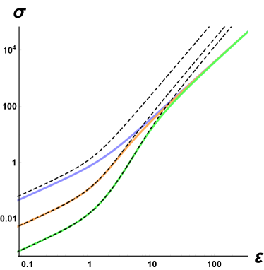
Figure 2: Left: Shear stress strain curve for various potentials and relative (dashed) large strain scaling at $m/T=1$. The potentials are chosen to have both stiffening and softening, i.e. $\nu_{1}^{S}=2\mathfrak{a}=4,2,2,0.2$ and $\nu_{2}^{S}=3\,\mathfrak{a}/\mathfrak{b}=3/2,1,3/5,1/7$. Here the constraints on the strain are not taken into account. Right: Shear stress strain curves of a potential $W(X,Z)=X^{2}\sqrt{Z}$ for different temperatures ($T/m=0.1,0.5,1$ for blue, orange and green) and comparison with the analytic formula (35) (dashed lines). As expected for $T/m\gg 1$ the formula gives a very good approximation.

At asymptotically large strain, $\varepsilon\gg 1$, it is still possible to obtain the non-linear scaling at large strain analytically by analysing the equations of motion (3.1). Large strain implies $\Omega\gg 1$ and so the tensor mode profile $h(u)$ is expected to perform a large excursion or, equivalently, to have sizeable gradient $h^{\prime}(u)$. It is convenient to introduce

$$\tilde{h}(u)\equiv\Omega-h(u)$$ (44)

because the potential depends on $h(u)$ only through this combination. At large $\Omega$, near the boundary this quantity is large, and moreover one can expect that $\tilde{h}^{\prime}(u)$ is also large (say, compared to $f^{\prime}(u)$) somewhere in the bulk.

The large $\tilde{h}\gg 1$ approximation allows to substitute $\cosh(\tilde{h})$ and $\sinh(\tilde{h})$ by $e^{\tilde{h}}/2$. If the potential $W(X,Z)$ is power-law-like as in our benchmark model, then it is easy to see that in this regime that the solution to the equations of motion (3.1) reaches a constant for $f(u)\simeq f_{0}<1$. In fact, our benchmark potential (36) admits a simple approximate solution of the form near the UV ($u\to 0$),

$$f(u)\,\simeq\,f_{0}=\frac{3\,\mathfrak{a}^{4}}{\left(\mathfrak{a}^{2}+\mathfrak{b}\right)\left(3\,\mathfrak{a}^{2}+\mathfrak{b}^{2}\right)}\;,\qquad\;\tilde{h}(u)\,\simeq\,-2\,\frac{\mathfrak{b}}{\mathfrak{a}}\,\log\left(\frac{u}{u_{0}}\right)\;,$$ (45)

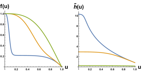
Figure 3: The metric functions $f(u)$ and $\tilde{h}(u)$ for a potential $W(X,Z)=X^{2}Z$, $u_{H}=1$, $\Omega=0.24,\,2.93,\,10.29$ and temperatures $T/m\sim 0.15,\,0.02,\,10^{-5}$ (Green, orange, blue).

with $m^{2}\;u_{0}^{2b}=3\,b\,2^{a}\,/(a^{2}+b)$. The logarithmic shape of $\tilde{h}(u)$ is clearly seen in Fig. 3.

Before discussing further the properties of this approximate solution, let us first see how it determines the elastic response at asymptotically large strain. In this limit, the function $\tilde{h}(u)$ at the UV is large but finite, $\tilde{h}(0)=\Omega$. Therefore, at some scale $u_{*}$, there must be a transition between the constant and the logarithmic profile (45). Assuming that (45) is correct up to the horizon, we have that approximately $\tilde{h}(u)\simeq\Omega-2\,\frac{\mathfrak{b}}{\mathfrak{a}}\,\log\left(\frac{u}{u_{*}}\right)$ from $u_{*}$ to $u_{H}$. This allows to identify $u_{*}$ as

$$u_{*}\,=\,u_{H}\,\exp\left(\frac{\mathfrak{a}}{2\,\mathfrak{b}}(\tilde{h}(u_{H})-\Omega)\,\right)\simeq\,u_{H}\,\exp\left(-\,\frac{\mathfrak{a}}{2\,\mathfrak{b}}\,\Omega\right)\,,$$ (46)

where in the last step we use that $\Omega\gg\tilde{h}(u_{H})$ which is reasonable since the $\tilde{h}$ variable is massive and ‘tries’ to reach 0. Thus, in the large strain limit, $\Omega\gg 1$, we have $u^{*}\rightarrow 0$. In other words, the intermediate solution (45) extends up to very close to the boundary. Since from the UV viewpoint $u_{*}$ represents the crossover scale where $\tilde{h}$ changes from constant to logarithmic behaviour, just from dimensional analysis one expects that the subleading term in the AdS UV expansion (31), $\mathcal{C}_{3}$, must scale like $\mathcal{C}_{3}\sim u_{*}^{-3}$. The shear strain is defined as $\varepsilon=2\sinh(\frac{\Omega}{2})$, thus the shear stress for a large shear strain will scale with $\nu_{2}^{S}\,=\,3\,\frac{\mathfrak{a}}{\mathfrak{b}}$ as indeed shown in fig.2.

Let us return now to the solution (45), which implies that the bulk metric in this limit takes a special form. Going to the coordinates $\tilde{x}$, $\tilde{y}$ where the metric is diagonal, the bulk asymptotic geometry is

$$ds^{2}\simeq\frac{1}{u^{2}}\left(\frac{du^{2}}{f_{0}}-u^{-2\mathfrak{b}^{2}/\mathfrak{a}^{2}}\,dt^{2}+u^{2\mathfrak{b}/\mathfrak{a}}d{\tilde{x}}^{2}+u^{-2\mathfrak{b}/\mathfrak{a}}d{\tilde{y}}^{2}\right)~{}.$$ (47)

This geometry represents a new UV fixed point. It is attractive towards the UV, but configurations with large enough strain get close to (47) for a long range in $\log\,u$. Interestingly, it exhibits both a Lifshitz dynamical exponent (between space and time directions) as well as a Lifshitz scaling with respect to $\tilde{x}$ and $\tilde{y}$ spatial directions – that is an anisotropic scaling. It is quite natural that for large strain the $x$ and $y$ directions become very anisotropic.

One might find more surprising that this occurs via a combined Lifshitz scaling both in the space and time directions. One way to understand this is by recalling that the models (13) can be thought of as massive gravity theories. Indeed, in the unitary gauge $\Phi^{I}=\delta^{I}_{j}\,x^{j}$ one has $X={\rm tr}\,g^{ij}$ and $Z={\rm det}\,g^{-1}$, so the scalar kinetic function $W(X,Z)$ becomes a potential for the (spatial part of the) metric. Recall that the simplest way to obtain a Lifshitz geometry is to support it with a massive spin-1 vector field Kachru:2008yh ; Taylor:2008tg ; Cremonini:2014pca . It is not so surprising, then that a massive spin-2 field can do a similar job.

Note that the existence of the anisotropic Lifshitz UV fixed point solution (47) depends slightly on the choice of the potential $W(X,Z)$. Looking at the first of Eqns. (3.1), one sees that a necessary condition for $f(u)=$const. to be a solution is that $h(u)$ is logarithmic. In turn, this gives room for $W$ either to approach a constant or to vanishing towards $u=0$. In order to be consistent with the second equation, this requires that $W_{h}$ (which at large $h$ translates into $XW_{,X}$) is constant along the solution. Since in these solutions $Z=u^{4}$, the only way that $XW_{,X}$ can reach constant is that it depends on $X,\,Z$ via the special combination $X^{p}\,Z^{q}$ with and $p\,,q$ constants which is such that every power of $Z$ can be compensated by the $X$- dependence. This is precisely what happens in our benchmark model (36). However it also happens in much more general choices of the form $W\big{(}X,Z\big{)}=W_{0}\big{(}X^{p}\,Z^{q}\big{)}$, with $W_{0}$ a free functions of one argument. (An additive function of $Z$ that vanishes at small $Z$ would lead to the same behaviour.) It is also clear that in a more generic potential that does not reduce to this form the anisotropic Lifshitz UV fixed point solution is not present. Still, one expects that some anisotropic solution (not completely scale invariant) should exist and dominate the response in the regime of asymptotically large strains.

In any case, the (near-)Lifshitz form of the geometry is expected to impact be seen also in transport properties like the electric conductivity at finite strain (see for example Bhattacharya:2014dea ). Therefore, this suggests an avenue to possibly test whether this anisotropic Lifshitz regime occurs in real materials.

Anisotropic models with a uni-directional scalar field $\phi=\alpha z$ have been already used extensively in the literature Mateos:2011ix ; Jain:2014vka ; Rebhan:2011vd . These models are expected to share some of the features of our solutions with large strain, as these can be represented by the scalars in the configuration $\Phi^{x}=\alpha\,e^{\Omega}$ and $\Phi^{y}=\alpha\,e^{-\Omega}$ in the limit $\Omega\to\infty$ keeping $\alpha\,e^{\Omega}$ fixed.

Elasticity bounds

Thus far, we have discussed how to extract and understand the stress-strain curve for the black branes with solid scalar hair (21). One can go one step further and give an estimate on the where the stress-strain curve should terminate. As explained in Alberte:2018doe , this can be done by studying the stability around the strained configuration. Generally speaking, this translates into a maximum strain $\epsilon_{max}$, beyond which the solutions have unstable perturbation modes which would render them unphysical.

The computation of the elasticity bound $\epsilon_{max}$ for the solids which can be described by EFT methods was presented recently in Alberte:2018doe . We are now ready to perform the analogous computation for our holographic solids that, as emphasized above, model the special case when scale invariance is a manifest – the solid is in a nontrivial fixed point.

To this end, one should study the stability of the strained solutions under small perturbations. In the context of black brane solutions, this proceeds by the computation of (the dispersion relation of) the quasi-normal modes (QNMs) for the solutions (22). This effort is beyond the scope of the present work, however we can already gain insight analyzing the perturbations in the decoupling limit.

More precisely, we will exploit the two following approximations. First, rather than working out the QNMs, we will look at the local propagation of fields in the bulk. At this level, it is much easier to identify when the propagation speed $c_{(i)}^{2}$ of some mode ‘$i$’ develops a wrong sign, $c_{(i)}^{2}<0$. By the local propagation speeds here we mean the coefficients in the $x,\,y$- gradient terms in the bulk equations of motion for the perturbations, which are functions of $u$. Certainly, the AdS boundary conditions are such that the QNMs might turn out to be stable modes even if some speed $c_{(i)}^{2}<0$ somewhere in the bulk. However, one expects that the threshold where the QNMs show an instability should be near the threshold where the first mode develops $c_{(i)}^{2}<0$ somewhere in the bulk. In any case, using this bulk criterion is expected to place a conservative upper bound on $\epsilon_{max}$.

On the other hand, we are going to work in the decoupling limit where the mixing between scalar perturbations $\delta\Phi^{I}$ with the metric modes is neglected. In this approximation, the equations for $\delta\Phi^{I}$ are completely parallel to those in a $2+1$ EFT in flat space – the exercise that was already done in Alberte:2018doe . On the configurations with finite strain (21) the phonon sound speeds are anisotropic, but one can still diagonalise the modes and thus obtain two characteristic speeds in the $(x,y)$ plane

$$c_{\pm}=c_{\pm}(\varepsilon,\varphi,u)$$ (48)

that depend on the strain magnitude $\varepsilon$, and on the angle $\varphi$ of propagation of the sound wave with respect to one of the the principal axes (eigendirections) of the strain tensor. The subscripts $\pm$ refer to the smallest and the largest of the two speeds. (In our holographic model, the speed in the holographic direction $u$ is always 1.)

The characteristic speeds are local, in the sense that they are defined at every slice $u=$const, but their structure in terms of the potential $W$ is identical to the one obtained in Alberte:2018doe . Moreover, for monomial potentials like (36), it is easy to see that the $u-$dependence disappears from characteristic speeds. A conservative implementation of a stability criterium against gradient instabilities, then, is that

$$c_{-}^{2}>0~{}$$ (49)

(for all angles $\varphi$). In fact, for the model (36), the local speeds in the $(x,y)$ plane depend on $\mathfrak{a},\,\mathfrak{b}$ in the very same way as how they depended on $A,\,B$ in the first benchmark model of Alberte:2018doe . The condition (49) reads exactly the same, however the physical role of the parameters is different.

This leads to a maximum strain deformation $\epsilon_{max}$ which reduces to a certain function of $\mathfrak{a},\,\mathfrak{b}$ for the model (36). In the following, we discuss the obtained results, by referring to physical parameters like the scaling exponents $\nu_{1,\,2}^{S}$ (Eqs. 41 and 42) instead of $\mathfrak{a},\,\mathfrak{b}$.

Note that both $\nu_{1,2}^{S}$ scaling exponents can be bigger and lower than $1$, meaning that both softening and stiffening can appear. Nevertheless the second scaling is always smaller than the first $\nu_{2}^{S}<2\mathfrak{a}$ because of consistency requirements (37).

Aside from the conditions shown in (37) that restrict the values of $\mathfrak{a}$ and $\mathfrak{b}$, we also find consistency conditions on the maximum shear strain that can be applied to the system, as mentioned above. From Fig. 4, we can already see that $\nu_{2}^{S}<\nu_{1}^{S}$, as expected. The upper bound to the maximum deformation $\epsilon_{max}$ comes from two different consistency conditions depending on the value of $\nu_{2}^{S}$: for the region $\nu_{2}^{S}>3$ we will first encounter ghosts (a change of sign in the kinetic term) at a finite value of shear strain, which will determine the value of $\varepsilon_{max}$, while in the region $\nu_{2}^{S}<3$ this value will be determined by a gradient instability (a change of sign in the speed $c_{-}^{2}$). There is a region with very large $\epsilon_{max}$ in between these two sectors, i.e. around $\nu_{2}^{S}\sim 3$, where it grows asymptotically. We can find the specific relation between $\epsilon_{max}$ and the shear scalings close to this area

$$\epsilon_{max}\sim\,\left(\frac{6}{|\nu^{S}_{2}-3|}\right)^{1/4}\,.$$ (50)

Surprisingly, the expression for the maximum deformation is the same either we are in above or below the value $\nu_{2}^{S}=3$, and it is independent of the value of $\nu_{1}^{S}$.

The subluminality constraint is also included Fig. 4, in the following way. The local speeds in the bulk (48) are allowed to be possibly superluminal, as the speeds in (48) do not give directly any physical phonon speeds. A proper limit would require the computation of the QNM dispersion relations at finite strain, which is outside the scope of this work. As a first step, though, we include the known results for the QNMs at vanishing strain Ammon:2019apj ; Baggioli:2019abx , which certainly places a bound and one expects it gives an idea of the kind of bound one should obtain. We thus cut out the white region, which is where the physical longitudinal phonon QNM would be superluminal at $\varepsilon=0$. By continuity, the true subluminality bound should make $\varepsilon_{max}$ vanish smoothly close to the edge of the white areas in Fig. 4. This has the effect to decrease $\varepsilon_{max}$ near the white edge and it should also render the actual plot less blue in the region $\nu_{1}^{B}\sim\nu_{1}^{B}\sim 6$, for instance. However, given the different slopes of the ‘blue ray’ and of the edge of the white area, one expects that the high elasticity region (the blue ray) persists mostly.

Figure 4: Left: Maximum shear strain, $\varepsilon_{max}$, as a function of the intermediate bulk and shear scaling, $\nu_{1}^{B}$ and $\nu_{1}^{S}$. There is one region with large $\varepsilon_{max}$ (large elasticity) around $\nu_{1}^{S}=\nu_{1}^{B}$. The limit in the strain at left and right of this region is also determined by requiring absence of gradient instability and ghosts respectively. In the white area, the longitudinal phonon is already superluminal at zero strain. Right: The same plot expressed in terms of the second shear scaling exponent $\nu_{2}^{S}$. (Notice that from (41), (42) and (53) we can write $\nu^{S}_{2}=3\;\nu^{S}_{1}/\nu^{B}_{1}$.) The region with asymptotically large $\varepsilon_{max}$ is around $\nu_{2}^{S}=3$.

Bulk deformations

We can as well consider the bulk response beyond the linear approximation. In this section, we will neglect the finite temperature corrections; as a consequence the results presented here are robust at small temperatures $T/m\ll 1$ but they will probably get finite $T$ corrections elsewhere. In order to compute the non linear bulk response and avoid mixing the different deformations we set the shear strain $\varepsilon=0$. In that case, the equilibrium configuration (25) is set by $\Phi^{I}=x^{I}$; this means that a bulk deformation $\kappa=\partial\cdot\phi$ corresponds to $\kappa=2(\alpha-1)$. Now, in analogy with linear response, we can compute the response in the pressure $T_{xx}=T_{tt}/2$, i.e. the longitudinal stress, with respect to the longitudinal strain in a full non linear form. We define the bulk stress as $\sigma_{L}=T_{xx}(\kappa)-T^{eq}_{xx}$. In more details for our model (36) we obtain:

$$\sigma_{L}(\kappa)\,=\,\frac{m^{2}\,\left(\left(\frac{\kappa}{2}\,+\,1\right)^{2\,\mathfrak{b}}\,u_{h,\kappa}^{2\,\mathfrak{b}\,-\,3}\,-\,u_{h,\kappa=0}^{2\,\mathfrak{b}\,-\,3}\right)}{2\,(2\,\mathfrak{b}\,-\,3)}\,+\,\frac{1}{2}\left(\frac{1}{u_{h,\kappa}^{3}}\,-\,\frac{1}{u_{h,\kappa=0}^{3}}\right)\,,$$ (51)

where with $u_{h,\kappa=0}$ we mean the value of the BH horizon in absence of any bulk strain, i.e. $\alpha=1$. The sign of $\kappa\equiv\partial\cdot\vec{\pi}$ can be positive, i.e. a compression, or negative, i.e. an expansion.
The results for various potentials are shown in fig.5. At large bulk strain $\kappa\gg 1$, we find a universal scaling

$$\sigma_{L}\,\propto\,\kappa^{3}\,,$$ (52)

which is a consequence of conformal invariance and it can be generalized to $\kappa^{D}$, with $D$ the number of spacetime boundary dimensions. The scaling can be immediately obtained analytically just realizing that in the limit $\kappa\gg 1$ the radius of the horizon scales like $u_{H}\propto 1/\kappa$ . Furthermore, this result is in perfect agreement with the EFT computations Alberte:2018doe . Similarly to what happens in shear deformation, at large temperatures, there is an in between scaling that goes as $\alpha^{2\mathfrak{b}}\,=\,\left(1+\frac{\kappa}{2}\right)^{2\mathfrak{b}}$, as can be seen in fig.5. Notice that there are again two types of deformation: isothermal ($T=const.$) and adiabatic ($s=const.$). In this last case, the scaling is always $\sigma_{L}\,\propto\,\kappa^{3}$, while the intermediate scaling only shows up for isothermal deformations.

Figure 5: Left: Non linear bulk elastic response for various potentials $W(X,Z)$ at small temperature $T/m=0.01$ (blue lines) and $T/m=1$ (red lines). At large deformations all the lines asymptote the universal scaling (52) $\sim\kappa^{3}$. At large temperatures there is a transition between linear and cubic scaling that grows as $\alpha^{2\mathfrak{b}}\,=\,\left(1+\frac{\kappa}{2}\right)^{2\mathfrak{b}}$. Right: Absolute value of $\sigma_{L}(\kappa)$ for $\mathfrak{a}=\mathfrak{b}=3$ and $T/m=0,1$ (blue, red) as a function of $-\,\kappa$.

Therefore, we can define two different bulk scalings, one that appears at intermediate strains and finite temperature and another that appears at very large strain or low temperatures, just like what happens for the shear deformation. These two bulk scalings are

$$\nu_{1}^{B}\equiv 2\,\mathfrak{b}\quad,\quad\nu_{2}^{B}\equiv 3\,,$$ (53)

where the first scaling is always equal or larger than the second: $\nu_{1}^{B}\geq\nu_{2}^{B}$.

So far, we have focused on bulk deformations with $\kappa>0$ but we have not discussed negative values of $\kappa$, i.e. expansion. In this case, in order to produce a full expansion we need to go to the limit where $\alpha\rightarrow 0$ which corresponds to $\kappa=-2$. We can see from (51) that for low temperatures the stress goes as $\sigma_{L}\sim(\alpha^{3}-1)=((\frac{\kappa}{2}+1)^{3}-1)$ and for temperatures high enough the scaling would be $2\mathfrak{b}$ instead of cubic. However, we do not get to see these non-linear scalings due to the short range of values $\alpha$ and $\kappa$ have during the expansion. A couple of examples at different temperatures are shown in the right panel of Fig. 5, where we just see a linear scaling that gets saturated at some finite value. There, we also find that the amount of stress needed to produce a full compression is finite. We are not aware of any experimental signature of scale invariance in the linear and non-linear elastic response. Our results suggest that scale invariance should play an important role, providing universal scaling which can be possible tested at quantum critical points or within the quantum critical region.

4 Solids with spontaneously broken scale invariance

In this section we present the analysis of the nonlinear response, for models of solids that realize scale invariance (SI) as a spontaneously broken symmetry. This case can be treated using EFT methods in Alberte:2018doe . Linear elasticity of this systems has been recently discussed in Baggioli:2019elg . The goal now is to extend the analysis to the nonlinear regime properties and to compare it with the manifest SI case studied in the previous section with AdS/CFT techniques.

4.1 Nonlinear response from EFT methods

In order to study the nonlinear response of a solid with spontaneously broken scale invariance we are going to employ EFT methods. We have already presented an EFT of a solid in (13), which has been studied in the past in Dubovsky:2011sj ; Nicolis:2013lma ; Nicolis:2015sra ; Alberte:2018doe , but now we want to consider only Lagrangians that are invariant under scale transformations. Therefore, we are going to demand that the Lagrangian that we introduced in (13) is invariant under

$$x^{\mu}\rightarrow\lambda^{-1}\,x^{\mu},\quad\phi^{I}\rightarrow\lambda^{\Delta}\phi^{I}\,,$$ (54)

with some ‘weight’ $\Delta$ for the fields $\phi^{I}$ that will depend on the potential, as can be seen in Baggioli:2019elg . We find that the most general potential that we can use must be of the form of

$$V_{SI}(X,Z)\,=\,Z^{\frac{1+\omega}{2}}\,f\left(x\right)\,,$$ (55)

with $x\equiv X/\sqrt{Z}$ and

$$\omega=\frac{1-(d-1)\,\Delta}{(d-1)(\Delta+1)}\,,$$

which is also identified as the equation of state parameter, $\omega=p/\rho$. Notice that, although the potentials (55) and (19) look alike, their relation is not trivial as the framework where they are used is completely different. The comparison between the two should be done through physical properties of the system they describe such as the non-linear scalings. Moreover, this potential is not describing a system with conformal invariance unless we take the particular case where $\omega=1/2$.

4.2 General results

The non-linear bulk scaling is determined by $\omega$ and is completely independent of the function $f(x)$. This scaling is given by

$$\nu_{B}=2\,(1+\omega)~{}.$$ (56)

Moreover, the bulk strain $\kappa$ is unconstrained, as opposed to the shear strain $\varepsilon$. Looking at Fig. 6, we can see that the case of a monomial potential the scaling is restricted to satisfy $2<\nu_{B}<4$. For a more general $f(x)$, we can find that the limit is still the same, i.e. we cannot have $\omega>1$ without gradient instabilities or superluminal modes. Thus, neither the non-linear bulk scaling nor the constraints of it depend on the shape of $f(x)$.

4.3 Benchmark models

The results related to the shear response are potential dependent, so we will need to specify what type of potential we want to study. In particular, we will take the two cases considered in Alberte:2018doe , which are:

1. The first possibility we will study is the case where $f(x)$ is a monomial, i.e.

   $$f(x)=x^{\nu_{S}/2}$$ (57)

   with $\omega$ as a free parameter. This simple potential realizes a power-law scaling in the stress for large deformations. This potentials will display a power-law behaviour in the stress-strain relation for the shear channel, which will be determined by $\nu_{S}$, i.e. we will have that at large deformations $\sigma_{S}\sim\epsilon^{\nu_{S}}$.

2. The second possibility we are going to consider is taking both

   $$f(x)=1+v^{2}x^{\nu_{S}/2}$$ (58)

   and the limit $\omega\rightarrow 0$. The advantage of this potential is that the speeds of the phonon modes will be realistic (i.e. much smaller than the speed of light) as long as $v^{2}\ll 1$, whereas the monomial potential has relativistic modes for generic values of $n$ and $\omega$. The shear response will only come from the $x$-dependent term, so the power-scaling of the shear response will be determined by $\nu_{S}$.

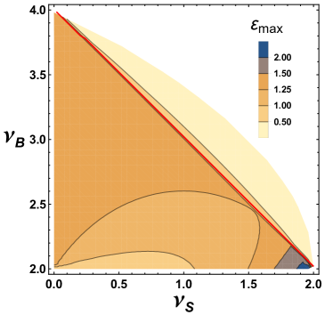
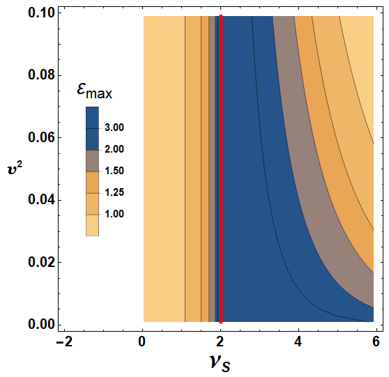
Figure 6: Left: The maximum allowed strain $\varepsilon_{max}$ within the allowed region for the monomial EFT case $f(x)=x^{\nu_{S}/2}$. The left, bottom and right edges are respectively given by: gradient instability, positivity of the bulk modulus and subluminality. The red line separates the region where $\varepsilon_{max}$ is controlled by gradient instability and subluminality. Right: The maximum allowed strain $\varepsilon_{max}$ within the allowed region. SSB case in the particular case where $\omega=0$ and $f(x)=1+v^{2}\,x^{\nu_{S}/2}$. The left and bottom edges are respectively given by: gradient instability and positivity of the bulk modulus. The maximum shear strain is determined by gradient instability for $\nu_{S}<2$, subluminality for $\nu_{S}>2$ and unconstrained for $\nu_{S}=2$.

The discussion about the shear scaling $\nu_{S}$ of the spontaneous broken scale invariance (SBSI) case is of course sensitive to the form of the function $f(x)$. The simplest non-trivial example of potential one can think of is a monomial, ie. $f(x)=x^{\nu_{S}/2}$, which is shown in Fig.6. In this particular scenario both the bulk and shear scalings are constrained, in particular we find that $2<\nu_{B}<4$ and $0<\nu_{S}<2$. As with the solids with manifest scale invariance, here we can find one region where the maximum strain sustained by the material is significantly large. The most elastic region is found close to $\nu_{S}\sim 2$ and we find that for this scaling $\varepsilon_{max}$ reads as

$$\varepsilon_{max}\simeq\sqrt{2}\,\left(\frac{1}{2-\nu_{S}}\right)^{1/4}\quad\mbox{for}\quad\nu_{S}\lesssim 2\,.$$ (59)

The problem with this kind of potentials is that the speeds of the phonons are excessively large. Typically one would expect that the speeds of these modes are not bigger than $\sim 10^{-4}$ times the light speed in ‘earthly’ materials (needless to say, this concern does not affect relativistic solids such as neutron star interiors). This constrains very much the possible scalings one can realize in a realistic scenario, specifically we would be restricted to $\nu_{S}$ and $\nu_{B}-2$ not bigger than $10^{-8}$.

If we do not restrict ourselves to the most simple case, we can describe a solid with slower phonon modes. For this, we are going to take $\omega\rightarrow 0$ and $f(x)=1+v^{2}\,x^{\nu_{S}/2}$ with $v^{2}\ll 1$ as proposed in Alberte:2018doe . This form of potential ensures that the speed of the phonon modes are small at least for small shear strain. The shear scaling is forced to be positive $\nu_{S}>0$ and the maximum shear scaling is

$$\nu_{S}^{max}=\frac{2\,(1+v^{2})}{v^{2}},$$ (60)

thus $\nu_{S}^{max}\gg 1$ for $v^{2}\ll 1$. The region with $\epsilon_{max}$ large is found around $\nu_{S}\lesssim 2$ and also in the region where $\nu_{S}>2$ and $v^{2}\ll 1$, specifically

$$\varepsilon_{max}\simeq\,\sqrt{2}\,\left(\frac{1}{2-\nu_{S}}\right)^{1/4}\quad\mbox{for}\quad\nu_{S}\lesssim 2\,,$$ (61)

$$\varepsilon_{max}\simeq\,\sqrt{2}\,\left(\frac{2}{v^{2}\,(\nu_{S}-2)}\right)^{\frac{1}{\nu_{S}}}\quad\mbox{for}\quad\nu_{S}\gtrsim 2\,,$$ (62)

where we have taken the limit $\omega\rightarrow 0$ and the last $\epsilon_{max}$ is valid for $\nu_{S}>2$ not necessarily close to $\nu_{S}=2$ as long as $v^{2}\ll 1$, as can be seen in Fig.6.

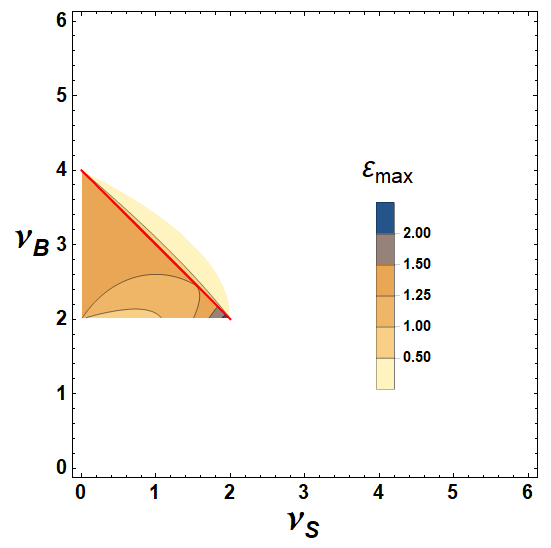
Figure 7: Summary of the main differences between the nonlinear elasticity bounds found for materials with spontaneously broken (left) or manifest (right) scale invariance. Both materials present power-law stress-strain relations $\sigma\sim\varepsilon^{\nu}$ (at $\varepsilon\gg 1$) with exponents $\nu^{B}$ and $\nu^{S}$ for pure-bulk and pure-shear deformations. Both the values of the maximum allowed deformation $\varepsilon_{max}$ as well as the range of values of the allowed exponents differ substantially.

5 Comparison

Let us now compare the nonlinear response obtained in the manifest/spontaneously broken SI cases. In order to make the comparison as meaningful as possible, we will fix the physical observable – the stress-strain curve to be of the type $\sigma\sim\epsilon^{\nu}$ for both bulk and shear deformations with exponents $\nu_{S,\,B}$ – and compare the elasticity bounds in the manifest or spontaneously broken case. Our holographic examples present two power-law regimes, but we will restrict attention to the first (‘intermediate’) one labeled with exponents $\nu_{1}^{S,\,B}$ because the second one is only realized at extremely large deformations (at finite temperature).

The results shown in Sections 3 and 4 make manifest that the universal elasticity bounds that can be obtained from low-energy effective methods differ significantly depending on how scale invariance is realized (as a manifest or a spontaneously broken symmetry). The main differences are basically summarized in Fig. 7, where we repeat here the relevant plots in Figs.4 and 6 but in a comparable scale, for the sake of comparison.

It is clear from Fig. 7, the elasticity bounds present substantial differences, both in the range of allowed values in the $\nu_{S}-\nu_{B}$ plane where finite deformations can be reached ($\varepsilon_{max}\sim 1$), as well as in the region where the deformations can be large ($\varepsilon_{max}\gg 1$).

In fact, if we restrict the CFT analysis to the models that exhibit massless phonons (which requires $\nu_{1}^{B}>5$) then the areas in the $\nu_{S}-\nu_{B}$ plane are almost disconnected, with the spontaneously broken case covering lower values of $\nu_{B}$ – globally in the $2<\nu_{B}<4$ window.

Similarly, the shear exponent is constrained to $0<\nu_{S}<2$ for the SB case while it is basically unbounded in the manifest case. Another major difference is the presence in the manifest case of a ‘very elastic band’ (the bluish area) in the region near

$$\nu_{1}^{S}=\nu_{1}^{B}~{}.$$ (63)

This is the region that allows for black rubber - like holographic duals. It is worth to emphasize two properties about these solutions: i) the band in parameter space start at $\nu_{1}^{B,\,S}\gtrsim 6$ which corresponds to a rather stiff behaviour; ii) these values of $\nu_{1}^{B,\,S}$ are far from the free scalar limit ($\mathfrak{a}=\mathfrak{b}=1$, corresponding to $\nu_{1}^{B,\,S}=2$). Thus, black rubbers require the presence of scalars with non-canonical (non-linear) kinetic terms in the bulk.

For the EFTs of Sec. 4 instead, the hyper-elastic region collapses down from a strip to basically a ‘dot’-like area. Let us remark that this last feature happens in the first EFT benchmark (57) but not in the second one (58) (which displays small sounds speeds and also an elastic band at $\nu_{1}^{S}\sim\nu_{1}^{B}$). However, we prefer to keep the comparison at this level because the benchmark (58) depends on an extra parameter.

As mentioned above, the reason to introduce the second benchmark model for in Sec. 4 is to be able to have realistic phonon speeds – much smaller than the speed of light $c$. A fair question, then, is whether this is also possible in the AdS/CFT framework or we are forced to have phonon speeds of the order of $c$. This issue has been already addressed in Baggioli:2019elg , where it is claimed that a solid with manifest SI and small phonon speeds is achievable. In the holographic set-up the speeds of the phonons are obtained by finding the spectrum of the quasi-normal modes, which have the form

$$\omega=c_{s}k-i\,D\,k^{2}\,\dots$$ (64)

for both transverse and longitudinal modes, as checked in Alberte:2017oqx ; Ammon:2019apj . The low energy dynamics of these solids with manifest SI are described by a low energy CFT (and thus an IR fixed point). It is conceivable that the Lorentz group that emerges in the IR has a different light-cone speed $c_{e}$, and thus the space-time metric is $ds_{e}^{2}=-c_{e}^{2}\,dt^{2}+dx^{i}dx_{i}$. This has a crucial impact in (64) if we compare the results between a Lorentz invariant theory with a light-cone speed $c$ and one with $c_{e}$, as we will obtain a rescaling in the dispersion relation as $\omega\rightarrow(c/c_{e})\,\omega$. Therefore, for $c_{e}\ll c$ the phonon speeds would get suppressed as

$$c_{s}\rightarrow\frac{c_{e}}{c}\,c_{s}\,\ll c\,.$$ (65)

If this is the case, we could also have a “realistic” solid with smaller speeds and, in addition, the white areas –limited by superluminal constraints– in Figure 4 would be enlarged.

6 Conclusions

We have analyzed the nonlinear elastic response in materials with scale invariance from the low-energy perspective, using effective field theory and holographic methods. The advantage in these effective methods is that they are mainly based on how symmetries are realized and therefore they can help to understand the nonlinear behaviour ‘universally’, that is, independently of the microscopic details of the material. The constraints imposed by how symmetries are realized imply nontrivial relations among different low-energy observables, especially the ones that encode the non-linear structure of the theory — the interactions in the material.

In order to illustrate the appearance of these constraints from the low energy theories (and their dependence on how symmetries are realized), we have focused on the example provided by the elasticity bounds: the maximum deformability that a material may withstand in a reversible form. These were discussed in Alberte:2018doe in the case for materials with no manifest scale invariance. In this work, we have obtained these bounds for scale invariant (SI) materials, which can be of two types: with manifest SI or with spontaneously broken SI. The latter case can be described using the EFT methods and so is a particular case of those discussed in Alberte:2018doe . For the manifest SI case, instead, we have used holographic models. In order to include the two key ingredients (elasticity and manifest scale invariance), we have studied the simple holographic models of ‘massive gravity’ type. These are well-defined effective field theories in (asymptotically) AdS spacetime and they allow for a straightforward interpretation as a scale invariant field theories.

The main result of this work is to show how the elastic response can be extended to the full non-linear regime by obtaining the full stress-strain curves. The procedure is straightforward, and it gives rise to a very rich phenomenology of nonlinear elasticity behaviours which can easily be extended to other holographic models.

To our knowledge, this is the first time that the full non-linear elastic response of AdS black brane geometries is presented by extracting the corresponding stress-strain curve. Previous studies have discussed the elastic response only in the linear approximation. Ref. Baggioli:2019mck discussed the visco-elastic oscillatory (that is, non-static) response and Biasi:2019eap an out-of-equilibrium similar setup.

As in Alberte:2018doe , in order to make progress, we have assumed models that, by assumption, display power-law stress-strain curves, $\sigma(\varepsilon)\sim\varepsilon^{\nu}$ with some constant exponent $\nu$ at large strains $\varepsilon\gg 1$. We have constructed the stress-strain curve and also followed how the appearance of pathologies (gradient instability, ghosts, or superluminal propagation) appears as a function of $\varepsilon$. We have then obtained how the maximum strain $\varepsilon_{max}$ depends on the exponents $\nu^{S}$ and $\nu^{B}$ (for shear and bulk transformations respectively).

We highlight three aspects of our obtained results. First, we find that the elasticity bounds for the solids with manifest SI (the holographic models) differ substantially from the ones for the solids with spontaneously broken SI (the EFT models), as shown clearly in Fig. 7. Both the ranges of allowed exponents and the values of the deformability $\varepsilon_{max}$ disagree by $\mathcal{O}(1)$ factors. Our interpretation of this discrepancy is that it is physical and due to the fact that SI is realized differently in the two cases, implying that the nonlinear constraints in the theories must differ.

The second aspect to illustrate is that our holographic models present the interesting peculiarity that they exhibit actually two different regimes of power-law stress-strain curves, $\sigma(\varepsilon)\sim\varepsilon^{\nu}$, with different exponents at moderately large $\varepsilon$ (say, $1<\varepsilon<10$) and asymptotically large $\varepsilon$. This is due to the fact that these models contain a UV anisotropic Lifshitz fixed point. It is unclear whether this feature is only specific to the present model or whether it should be more generic in (very) elastic solids with manifest SI. Neither it is clear how relevant this feature is for realistic materials as this second scaling regime only appears for extremely large deformations, $\varepsilon\gtrsim 10$, before which the solutions already show some instability.

Finally, we stress that the holographic models that exhibit highest elasticity share features surprisingly similar to familiar real-world elastomers. Indeed, the models that allow black brane solutions which are stable under largest deformations (largest $\varepsilon_{max}$) turn out to have power-law exponents $\nu$ in the stress-strain curves $\sigma\sim\varepsilon^{\nu}$ which are: i) of order a few; ii) similar for pure-shear and pure-bulk $\nu_{S}=\nu_{B}$ (corresponding to the blue stripe in Fig 7.b). Intriguingly, this is what happens for natural rubber and other elastomers enlighten70333 – and it motivates us to call these solutions black rubber.

Very importantly we would like to comment on the possible applications of this framework to realistic systems.

(I) The electric transport properties of quantum critical materials have been subject of lot of recent efforts especially in connection to the “anomalous” scalings found in Strange metals. More recently the question whether also phonons and elastic properties can display surprising and interesting features in quantum critical materials has emerged. More specifically there are preliminary indications that phonons in quantum critical systems can exhibit glassy or viscoelastic features ishii2019glass . Moreover the role of these viscoelastic properties has been discussed in connection to the possible implications on the onset of (high-Tc) superconductivity setty2019glass . The framework just presented can provide a useful methods and possible observable predictions in this directions. The utility of these holographic models has been already proven in understanding the glassy features of amorphous solids and ordered crystals in Baggioli:2018qwu ; baggioli2018soft ; baggioli2019unified .

(II) Let us also mention the growing interest related to the non-linear mechanical characterization of critical materials (e.g. High-$T_{c}$ superconductors) due to their technological applications Scheuerlein:2017kjv ; Scheuerlein:2017zka . Given the absence of robust computational methods, one may not rule out that the holographic methods such as presented here may provide useful insights.

(III) Following Baggioli:2019mck , a full non-linear characterization of the mechanical response of the holographic homogeneous models Baggioli:2014roa considered in this work could definitely shed light on their physical nature, which is still open Ammon:2020xyv ; Baggioli:2020nay .

Finally, we remark a perhaps more technical point that we think is interesting from the gravitational point of view. The computation of the mechanical response to non-linear shear deformations translates in the AdS/CFT dictionary into finding exact black hole solutions with finite shear deformation (and shear stress) in the transverse directions. This implies that these solutions have a non-trivial, nonlinear spin-2 mode, and we devoted some effort to derive them in Sec. 3. These solutions are similar to the nonlinear gravitational waves and ‘pp-wave’ solutions in General Relativity in that they also have a nonlinear spin-2 (transverse-traceless) mode However, in our models the solutions are static, which is a direct manifestation of the massive character of the metric in these models. Moreover, the spin-2 mode ‘sticks out’ of a black brane horizon. In this sense, then, these solutions can be thought of as branes with spin-2 hair. We are unaware of solutions of this kind in the literature, but we find it remarkable that they are exist, and are tied to the nonlinear elastic response.

Appendix A Holographic Stress Tensor

We can explicitely compute the boundary stress tensor $T^{\mu\nu}$ following Balasubramanian:1999re . In particular, for asymptotic AdS₄ spacetime, we have:

$$T^{\mu\nu}\,=\,\frac{1}{8\,\pi\,G}\,\left(\Theta^{\mu\nu}\,-\,\Theta\,\Xi^{\mu\nu}\,-\,2\,\Xi^{\mu\nu}\,-\,G^{\mu\nu}_{\Xi}\right)\,,$$ (66)

where we set the AdS length $l=1$. The metric $\Xi_{\mu\nu}$ is the boundary metric and $\Theta^{\mu\nu}$ the extrinsic curvature of the boundary surface, with $\Theta$ its trace. Our boundary metric is given by

$$\Xi_{ij}=\frac{1}{u^{2}}\begin{pmatrix}e^{-\chi(u)}\,f(u)&0&0\\ 0&\cosh h(u)&\sinh h(u)\\ 0&\sinh h(u)&\cosh h(u)\end{pmatrix}$$ (67)

and it is clearly flat, implying $G^{\mu\nu}_{\Xi}=0$. We can define the normal vector to the boundary as:

$$n_{\mu}\,=\,\left(0\,,\,0\,,\,0\,,\,\frac{1}{\sqrt{g^{uu}}}\right),$$ (68)

where $g^{uu}=u^{2}f(u)$. The extrinsic curvature can be defined as usual

$$\theta_{\mu\nu}\,=\,\frac{1}{2}\left(\nabla_{\mu}n_{\nu}\,+\,\nabla_{\nu}n_{\mu}\right),$$ (69)

and it reads

$$\theta\,=\,\frac{u\,f^{\prime}(u)\,-\,f(u)\,(6\,+\,u\chi^{\prime}(u))}{2\sqrt{f(u)}}.$$ (70)

Close to the boundary, we can expand the function $h(u)$ as in (31) and $f(u)=1-M(u)u^{3}$ (where $M(0)$ would correspond to the energy density of the system) and find that the off-diagonal component of the stress-energy tensor is

$$T_{xy}\,=\,\frac{1}{2}\left(3\,\mathcal{C}_{3}\cosh\left(\mathcal{C}_{0}\right)\,+\,M(0)\sinh(\mathcal{C}_{0})\right)$$ (71)

This result is a direct manifestation of the presence of a strain deformation in our background and it will encode the corresponding response, i.e. the shear component of the stress.
Interestingly one can also notice that

$$T_{x}^{\ y}\,=\,\frac{3}{2}\mathcal{C}_{3}.$$ (72)

Using the standard holographic renormalization techniques Skenderis:2002wp we can also identify

$$T_{\mu\nu}\,=\,\frac{3}{2}g_{\mu\nu}^{(3)},$$ (73)

where $g_{\mu\nu}^{(3)}$ is the sub-leading term of the induced metric expressed in Fefferman-Graham coordinates. As a first step we have to rewrite our ansatz in the FG form using the coordinate transformation

$$\frac{dz^{2}}{z^{2}}\,=\,\frac{du^{2}}{u^{2}\,f(u)}$$ (74)

where $z$ will now be the holographic (FG) coordinate.

Again, using that the asymptotic behaviour of $f(u)$ is $1-M(u)u^{3}$ we can find that for small $z$ we have $u=z-\frac{M(z)z^{4}}{6}$. Now we can already look at our metric and derive the stress-energy tensor. For instance, for the off-diagonal term, we are interested in, we have

$$g_{xy}(z)\,=\,\frac{1}{u(z)^{2}}\sinh(h(u(z)))=$$ (75)

$$=\,\frac{1}{z^{2}}\left(\cosh(\mathcal{C}_{0})+\left(3\,\mathcal{C}_{3}\cosh\left(\mathcal{C}_{0}\right)\,+\,M(0)\sinh(\mathcal{C}_{0})\right)z^{3}\right),$$ (76)

where higher orders in $z$ have been suppressed. We can identify $T_{xy}$ easily in this expression and see that the result is the same we found before in 71. This result give us a robust definition of the non-linear stress in our system which can be indeed identified as:

$$\sigma\,=\,\frac{1}{2}\left(3\,\mathcal{C}_{3}\cosh\left(\mathcal{C}_{0}\right)\,+\,M(0)\sinh(\mathcal{C}_{0})\right)$$ (77)

Since we impose the boundary condition $\mathcal{C}_{0}=0$ the stress, we use in all our computations, is simply defined by $\sigma\,=\,\frac{3}{2}\,\mathcal{C}_{3}$.

Appendix B Three-phonon interaction terms in Solid EFTs

To further illustrate the predictive power of the low energy methods, we show here another nontrivial powerful statement that follows from the EFT construction which, as explained above, applies when translations (and possibly scale invariance) are broken spontaneously.

The nontrivial statement contained in the EFTs (13) is simply that once the stress-strain relations are known then the full Lagrangian is fixed. Let us illustrate now how this impacts for instance in the determination of the cubic phonon interactions. Assuming that the stress-strain relations both for bulk and shear deformations are known, then one can reconstruct the full form of the function $V(X,Z)$ Alberte:2018doe , up to an irrelevant additive constant.

Then, the cubic phonon interactions (around the homogeneous, isotropic equilibrium configuration $\phi^{I}=x^{I}$) are obtained by expanding our Lagrangian around the background solution, i.e. $\phi^{I}=x^{I}+\pi^{I}$. At third order in $\pi^{I}$ we obtain

$$\begin{split}V(X,Z)\Rightarrow&\,\,\mathcal{C}_{1}\,(\partial_{i}\pi^{i}_{L})^{3}+\mathcal{C}_{2}\,(\partial_{i}\pi^{i}_{L})\,(\dot{\pi}_{j})^{2}+\mathcal{C}_{3}\,(\partial_{i}\pi^{i}_{L})\,(\partial_{j}\pi_{k})^{2}\\ &+\mathcal{C}_{4}\,\dot{\pi}^{i}\,\dot{\pi}^{j}\,\partial_{i}\pi_{j}+\mathcal{C}_{5}\,(\partial_{i}\pi^{i}_{L})\,(\partial_{j}\pi_{k})\,(\partial_{k}\pi_{j})\,,\end{split}$$ (78)

where $\pi^{I}=\pi^{I}_{L}+\pi^{I}_{T}$. The terms we find are

$$\mathcal{C}_{1}=\frac{1}{6}\left(8\,V_{ZZZ}+12\,V_{XZZ}+6\,V_{XXZ}+V_{XXX}\right)+4\,V_{ZZ}+2\,V_{XZ}+V_{Z}\,,$$ (79)

$$\mathcal{C}_{2}=-2\,V_{ZZ}-\frac{1}{2}\,V_{XX}-4\,V_{Z}-2\,V_{XZ}\,,$$ (80)

$$\mathcal{C}_{3}=\frac{1}{2}\,V_{XX}+\,V_{XZ}\,,$$ (81)

$$\mathcal{C}_{4}=2\,V_{Z}\,,$$ (82)

$$\mathcal{C}_{5}=-2\,V_{ZZ}-V_{Z}-V_{XZ}\,.$$ (83)

In these expressions, the $X,\,Z$- derivatives of $V$ are evaluated on the undeformed configuration. Moreover, by obtaining the relation between $V(X,Z)$ and the stress-strain curve (such as e.g. Eq. (18)) one can relate all these $V(X,Z)$ derivatives to derivatives of the stress strain curve at the origin, $\sigma^{\prime}(0)$, $\sigma^{\prime\prime}(0)$, etc, which are measurable quantities. For instance, the bulk modulus is ${\cal K}=4V_{ZZ}+2V_{Z}+4V_{XZ}+V_{XX}$, $\mathcal{G}=V_{X}$ and $\epsilon+p=V_{X}+2V_{Z}$.

This illustrates that the realization of symmetries implies nontrivial relations between distinct low energy observables. In this example, the strength of the phonon cubic interactions are determined by the shape of the stress-strain curves.

We can write the 5 $\mathcal{C}$’s as a function of these quantities and we would just need two independent new parameters

$$\mathcal{C}_{1}=\frac{\mathcal{K}}{2}+\mathcal{N}\,,$$ (84)

$$\mathcal{C}_{2}=\frac{1}{2}\left(3\,\mathcal{G}-\mathcal{K}-3\,(\epsilon+p)\right))\,,$$ (85)

$$\mathcal{C}_{3}=\frac{1}{4}\left(\mathcal{G}+\mathcal{K}-(\epsilon+p)\right)+\mathcal{M}\,,$$ (86)

$$\mathcal{C}_{4}=\epsilon+p-\mathcal{G}\,,$$ (87)

$$\mathcal{C}_{5}=\frac{1}{4}\left(\mathcal{G}-\mathcal{K}-(\epsilon+p)\right)+\mathcal{M}\,.$$ (88)

where the independent new parameters are

$$\mathcal{N}=\frac{1}{6}\left(8\,V_{ZZZ}+12\,V_{XZZ}+6\,V_{XXZ}+V_{XXX}\right)-2\,V_{ZZ}-\frac{1}{2}\,V_{XX}\,,$$ (89)

$$\mathcal{M}=\frac{1}{4}\,V_{XX}-V_{ZZ}\,.$$ (90)

We can compare our results with Ref. Leutwyler:1996er . There he concludes that there are 3 independent new parameters, but we think the difference comes from the fact that he is working in 3 space-dimensions instead of 2. Moreover, in Ref. Leutwyler:1996er there are 6 independent operators in the cubic expansion. It is trivial to check that in two dimensions the extra operator can be expressed as a function of the others

$$(\partial_{i}\pi_{j})\,(\partial_{i}\pi_{k})\,(\partial_{j}\pi_{k})=(\partial_{i}\pi^{i})\,(\partial_{j}\pi_{k})^{2}+\frac{(\partial_{i}\pi^{i})}{2}\,\left((\partial_{j}\pi_{k})(\partial_{k}\pi_{j})-(\partial_{i}\pi^{i})^{2}\right)\,.$$ (91)

In the case of scale invariance these terms simplify considerably. Let us then take $V(X,Z)=Z^{\frac{1}{2}+\omega}\,f\left(\frac{X}{\sqrt{Z}}\right)$

$$\mathcal{C}_{1}=\frac{\omega}{3}\left((2+6\,\omega+4\,\omega^{2})f(1)-3f^{\prime}(1)\right)\,,$$ (92)

$$\mathcal{C}_{2}=\frac{1}{2}\left(-(3+8\,\omega+4\,\omega^{2})\,f(1)+3\,f^{\prime}(1)\right)\,,$$ (93)

$$\mathcal{C}_{3}=\omega\,f^{\prime}(1)\,,$$ (94)

$$\mathcal{C}_{4}=(1+2\omega)\,f(1)-f^{\prime}(1)\,,$$ (95)

$$\mathcal{C}_{5}=\omega\,(f^{\prime}(1)-(1+2\,\omega)\,f(1))\,.$$ (96)

This implies that for a scale invariant potential there are no free parameters: we can identify $f(1)$, $f^{\prime}(1)$ and $\omega$ with $\mathcal{K}$, $\mathcal{G}$ and $\epsilon+p$

$$\mathcal{G}=f^{\prime}(1)\,,$$ (97)

$$\mathcal{K}=2\,\omega\,(1+2\,\omega)\,f(1)\,,$$ (98)

$$\epsilon+p=(1+2\,\omega)\,f(1)\,.$$ (99)

Therefore cubic interactions are all fixed by these background or linear elasticity quantities. This is true both for general SI as well as conformal solid limit (which is just a particular value of $w$).

References

- (1) L. D. Landau and E. M. Lifshitz, Course of Theoretical Physics, Vol. 7,Theory of Elasticity. Pergamon Press, 1970.
- (2) P. M. Chaikin and T. C. Lubensky, Principles of Condensed Matter Physics. Cambridge University Press, 1995, 10.1017/CBO9780511813467.
- (3) R. W. Ogden, G. Saccomandi and I. Sgura, Fitting hyperelastic models to experimental data, Computational Mechanics 34 (Nov, 2004) 484–502.
- (4) R. W. Ogden, Non-Linear Elastic Deformations. WILEY-VCH Verlag, 1985.
- (5) P. C. Martin, O. Parodi and P. S. Pershan, Unified hydrodynamic theory for crystals, liquid crystals, and normal fluids, Phys. Rev. A 6 (Dec, 1972) 2401–2420.
- (6) Y.B.Fu and R. Ogden, Nonlinear Elasticity: Theory and Applications. No. 283 in London Mathematical Society lecture note series. Cambridge University Press, Cambridge, UK, 2001, 10.1017/CBO9780511526466.
- (7) H. Leutwyler, Phonons as goldstone bosons, Helv. Phys. Acta 70 (1997) 275–286, [hep-ph/9609466].
- (8) S. Dubovsky, L. Hui, A. Nicolis and D. T. Son, Effective field theory for hydrodynamics: thermodynamics, and the derivative expansion, Phys. Rev. D85 (2012) 085029, [1107.0731].
- (9) A. Nicolis, R. Penco and R. A. Rosen, Relativistic Fluids, Superfluids, Solids and Supersolids from a Coset Construction, Phys. Rev. D89 (2014) 045002, [1307.0517].
- (10) A. Nicolis, R. Penco, F. Piazza and R. Rattazzi, Zoology of condensed matter: Framids, ordinary stuff, extra-ordinary stuff, JHEP 06 (2015) 155, [1501.03845].
- (11) L. Alberte, M. Baggioli, V. Cancer-Castillo and O. Pujolas, Elasticity bounds from Effective Field Theory, Phys. Rev. D100 (2019) 065015, [1807.07474].
- (12) M. Baggioli, V. C. Castillo and O. Pujolas, Scale invariant solids, 1910.05281.
- (13) L. Boyle, M. Dickens and F. Flicker, Conformal Quasicrystals and Holography, Phys. Rev. X 10 (2020) 011009, [1805.02665].
- (14) M. Baggioli, Homogeneous holographic viscoelastic models and quasicrystals, Phys. Rev. Research 2 (Apr, 2020) 022022.
- (15) M. Baggioli, Applied Holography: A Practical Mini-Course. SpringerBriefs in Physics. Springer, 2019, 10.1007/978-3-030-35184-7.
- (16) R. Emparan, T. Harmark, V. Niarchos and N. A. Obers, Essentials of Blackfold Dynamics, JHEP 03 (2010) 063, [0910.1601].
- (17) R. Emparan, K. Izumi, R. Luna, R. Suzuki and K. Tanabe, Hydro-elastic Complementarity in Black Branes at large D, JHEP 06 (2016) 117, [1602.05752].
- (18) D. Vegh, Holography without translational symmetry, 1301.0537.
- (19) M. Blake, D. Tong and D. Vegh, Holographic Lattices Give the Graviton an Effective Mass, Phys. Rev. Lett. 112 (2014) 071602, [1310.3832].
- (20) T. Andrade and B. Withers, A simple holographic model of momentum relaxation, JHEP 05 (2014) 101, [1311.5157].
- (21) M. Baggioli and O. Pujolas, Electron-Phonon Interactions, Metal-Insulator Transitions, and Holographic Massive Gravity, Phys. Rev. Lett. 114 (2015) 251602, [1411.1003].
- (22) L. Alberte, M. Baggioli, A. Khmelnitsky and O. Pujolas, Solid Holography and Massive Gravity, JHEP 02 (2016) 114, [1510.09089].
- (23) M. Ammon, M. Baggioli, S. Gray, S. Grieninger and A. Jain, On the Hydrodynamic Description of Holographic Viscoelastic Models, 2001.05737.
- (24) L. Alberte, M. Ammon, M. Baggioli, A. Jiménez and O. Pujolàs, Black hole elasticity and gapped transverse phonons in holography, JHEP 01 (2018) 129, [1708.08477].
- (25) L. Alberte, M. Ammon, M. Baggioli, A. Jiménez-Alba and O. Pujolàs, Holographic Phonons, 1711.03100.
- (26) L. Alberte, M. Baggioli and O. Pujolas, Viscosity bound violation in holographic solids and the viscoelastic response, JHEP 07 (2016) 074, [1601.03384].
- (27) M. Baggioli and A. Buchel, Holographic Viscoelastic Hydrodynamics, 1805.06756.
- (28) T. Andrade, M. Baggioli and O. Pujolas, Viscoelastic Dynamics in Holography, 1903.02859.
- (29) M. Baggioli, S. Grieninger and H. Soltanpanahi, Nonlinear Oscillatory Shear Tests in Viscoelastic Holography, 1910.06331.
- (30) M. Baggioli, Are The Homogeneous Holographic Viscoelastic Models Quasicrystals ?, 2001.06228.
- (31) M. Baggioli, Gravity, holography and applications to condensed matter. PhD thesis, Barcelona U., 2016. 1610.02681.
- (32) M. Baggioli and M. Goykhman, Phases of holographic superconductors with broken translational symmetry, JHEP 07 (2015) 035, [1504.05561].
- (33) M. Baggioli and D. K. Brattan, Drag phenomena from holographic massive gravity, Class. Quant. Grav. 34 (2017) 015008, [1504.07635].
- (34) M. Baggioli and M. Goykhman, Under The Dome: Doped holographic superconductors with broken translational symmetry, JHEP 01 (2016) 011, [1510.06363].
- (35) M. Baggioli and W.-J. Li, Universal Bounds on Transport in Holographic Systems with Broken Translations, 2005.06482.
- (36) Y. Bardoux, M. M. Caldarelli and C. Charmousis, Shaping black holes with free fields, JHEP 05 (2012) 054, [1202.4458].
- (37) M. M. Caldarelli, A. Christodoulou, I. Papadimitriou and K. Skenderis, Phases of planar AdS black holes with axionic charge, JHEP 04 (2017) 001, [1612.07214].
- (38) M. Ammon, M. Baggioli, S. Gray and S. Grieninger, Longitudinal Sound and Diffusion in Holographic Massive Gravity, JHEP 10 (2019) 064, [1905.09164].
- (39) M. Baggioli and S. Grieninger, Zoology of solid & fluid holography — Goldstone modes and phase relaxation, JHEP 10 (2019) 235, [1905.09488].
- (40) S. Kachru, X. Liu and M. Mulligan, Gravity duals of Lifshitz-like fixed points, Phys. Rev. D 78 (2008) 106005, [0808.1725].
- (41) M. Taylor, Non-relativistic holography, 0812.0530.
- (42) S. Cremonini, X. Dong, J. Rong and K. Sun, Holographic RG flows with nematic IR phases, JHEP 07 (2015) 082, [1412.8638].
- (43) J. Bhattacharya, S. Cremonini and B. Goutéraux, Intermediate scalings in holographic RG flows and conductivities, JHEP 02 (2015) 035, [1409.4797].
- (44) D. Mateos and D. Trancanelli, The anisotropic N=4 super Yang-Mills plasma and its instabilities, Phys. Rev. Lett. 107 (2011) 101601, [1105.3472].
- (45) S. Jain, N. Kundu, K. Sen, A. Sinha and S. P. Trivedi, A Strongly Coupled Anisotropic Fluid From Dilaton Driven Holography, JHEP 01 (2015) 005, [1406.4874].
- (46) A. Rebhan and D. Steineder, Violation of the Holographic Viscosity Bound in a Strongly Coupled Anisotropic Plasma, Phys. Rev. Lett. 108 (2012) 021601, [1110.6825].
- (47) M. Baggioli, B. Goutéraux, E. Kiritsis and W.-J. Li, Higher derivative corrections to incoherent metallic transport in holography, JHEP 03 (2017) 170, [1612.05500].
- (48) M. Baggioli and W.-J. Li, Diffusivities bounds and chaos in holographic Horndeski theories, JHEP 07 (2017) 055, [1705.01766].
- (49) A. Biasi, J. Mas and A. Serantes, Gravitational wave driving of a gapped holographic system, JHEP 05 (2019) 161, [1903.05618].
- (50) Y. Ishii, Y. Ouchi, S. Kawaguchi, H. Ishibashi, Y. Kubota and S. Mori, Glass-like features of crystalline solids in the quantum critical regime, arXiv preprint arXiv:1901.09502 (2019) .
- (51) C. Setty, Glass-induced enhancement of superconducting : Pairing via dissipative mediators, arXiv preprint arXiv:1902.00516 (2019) .
- (52) M. Baggioli and A. Zaccone, Universal origin of boson peak vibrational anomalies in ordered crystals and in amorphous materials, 1810.09516.
- (53) M. Baggioli and A. Zaccone, Soft optical phonons induce glassy-like vibrational and thermal anomalies in ordered crystals, arXiv preprint arXiv:1812.07245 (2018) .
- (54) M. Baggioli and A. Zaccone, Unified theory of vibrational spectra in amorphous materials, 2019.
- (55) C. Scheuerlein, F. Lackner, F. Savary, B. Rehmer, M. Finn and C. Meyer, Thermomechanical behavior of the HL-LHC 11 Tesla Nb3Sn magnet coil constituents during reaction heat treatment, 1711.07022.
- (56) C. Scheuerlein, F. Lackner, F. Savary, B. Rehmer, M. Finn and P. Uhlemann, Mechanical Properties of the HL-LHC 11 T Nb3Sn Magnet Constituent Materials, IEEE Trans. Appl. Supercond. 27 (2017) 4003007.
- (57) V. Balasubramanian and P. Kraus, A Stress tensor for Anti-de Sitter gravity, Commun. Math. Phys. 208 (1999) 413–428, [hep-th/9902121].
- (58) K. Skenderis, Lecture notes on holographic renormalization, Class. Quant. Grav. 19 (2002) 5849–5876, [hep-th/0209067].