Classification of critically fixed anti-rational maps

Abstract.

We show that there is a one-to-one correspondence between conjugacy classes of critically fixed anti-rational maps and equivalence classes of certain plane graphs. We furthermore prove that critically fixed anti-rational maps are combinatorially equivalent to “topological Schottky maps” associated to these graphs, given in each face by a topological reflection in its boundary. As a corollary, we obtain a similar classification of critically fixed anti-polynomials by certain plane trees. One of the main technical tools is an analogue of Thurston’s characterization of rational maps in the orientation-reversing case.

1. Introduction

Our object of study in this paper is orientation-reversing complex (holomorphic) dynamics. The prefix “anti-” (as in “anti-holomorphic”, “anti-conformal”, or “anti-Thurston map”) will always denote orientation-reversing versions of familiar concepts from complex analysis and complex dynamics. E.g., an anti-rational map is the complex conjugate of a rational map. Many of the results in holomorphic dynamics also hold in anti-holomorphic dynamics, but there are several subtle and not-so-subtle differences, see Section 2. Besides studying anti-holomorphic dynamics in the context and as an extension of complex dynamics, it has intriguing connections to Kleinian groups [LMM21, LLMM19, LLM22] and to the theory of gravitational lensing [KN08].

The main result in this paper is the classification of critically fixed anti-rational maps via certain plane graphs. The analogous problem for critically fixed rational maps was solved by Hlushchanka [Hlu19], following partial results in [CGN⁺15]. A classification of critically fixed anti-polynomials with simple critical points was obtained in [Gey08] for the case of real coefficients, and in [LMM21] for general complex coefficients. As a corollary of our result, we obtain a general classification of critically fixed anti-polynomials by certain plane trees, without any assumption on multiplicities of critical points.

The structure of this paper is as follows: After a review of anti-holomorphic dynamics, we prove an orientation-reversing version of Thurston’s theorem on the characterization of post-critically finite rational functions. In Section 4, we introduce Tischler graphs $T_{f}$ of critically fixed anti-rational maps $f$, which are plane graphs whose edges are the fixed internal rays in superattracting basins. These graphs were originally introduced in [Tis89] to study critically fixed polynomials, and they have played a crucial role in the classification results for critically fixed rational maps mentioned above. Our main result in this section is Theorem 4.3, describing the properties of the Tischler graph $T=T_{f}$ associated to a critically fixed anti-rational map $f$:

1. $T$ is a connected bipartite plane graph.

2. $T$ is forward invariant, i.e., $f(T)=T$.

3. The vertices of $T$ are exactly the fixed points of $f$, and each edge of $T$ connects a critical fixed point to a repelling fixed point.

4. Every repelling vertex of $T$ has degree 2, and every critical vertex has degree $m+2\geq 3$, where $m$ is the multiplicity of the critical point.

5. Every face $A$ of $T$ is a Jordan domain, and $f$ maps $A$ anti-conformally onto $\mathbb{\hat{C}}\setminus\overline{A}$.

Following this, in Section 5 we define topological Tischler graphs as connected plane graphs $T\subset S^{2}$ where every vertex has degree $\geq 3$, and each face is a Jordan domain. Here we discard the repelling vertices, since they all have degree 2, but we do allow multiple edges. (In principle, by removing all vertices of degree 2, we could also introduce loops, but it is easy to see that this would contradict the assumption that all faces are Jordan domains.) For every topological Tischler graph $T$ we associate a Schottky map $f_{T}$ as a map whose restriction to every face $A$ of $T$ is a topological reflection (see Definition 5.3) in its boundary $\partial A$. In particular, $f$ is the identity on $T$, and it is an orientation-reversing branched cover of the sphere, whose branch points are exactly the vertices of $T$. The main results in this section are Theorems 5.6 and 5.9, and Corollary 5.12:

1. Every critically fixed anti-rational map with Tischler graph $T$ is (combinatorially) equivalent to the Schottky map $f_{T}$.

2. A Schottky map $f_{T}$ is (Thurston) obstructed if and only if there is a pair of faces $A$ and $B$ of $T$, whose boundaries share a pair of distinct edges $a,b\in\partial A\cap\partial B$.

3. Unobstructed Schottky maps $f_{T}$ and $f_{T^{\prime}}$ are equivalent if and only if the graphs $T$ and $T^{\prime}$ are equivalent.

Combined with the orientation-reversing version of Thurston’s theorem, this shows that there is a one-to-one correspondence between equivalence classes of unobstructed topological Tischler graphs and Möbius conjugacy classes of critically fixed anti-rational maps. As a corollary of the uniqueness, we show that symmetries of topological Tischler graphs are inherited by the equivalent anti-rational maps.

In Section 6, we use this to characterize critically fixed anti-polynomials via topological Tischler trees, which can be thought of as topological versions of either the Tischler graph with the vertex at $\infty$ removed, or as an extension of Hubbard trees for polynomials. Making life even easier for anti-polynomials, we prove that Tischler trees are never obstructed.

Finally, Section 7 contains a list of examples of small degrees, as well as an application to maps with symmetries.

A similar, closely related, and ultimately equivalent classification of critically fixed anti-rational maps was obtained independently in [LLM22]. See also [Par22], where an equivalent characterization of obstructions for Schottky maps was obtained as an application of a more general framework.

Lastly, discussions, feedback, and encouragement from many people considerably improved this paper. Special thanks are due to Mikhail Hlushchanka who beyond lots of feedback showed me a significant simplification of the proof of Theorem 4.3, and to Chris McKay who suggested many improvements and corrections in all parts of the paper. I am also indebted to the organizers and other participants of the MSRI special program on Complex Dynamics in Spring 2022, and the Department of Mathematical Sciences at Montana State University (and in particular our department head Beth Burroughs) who supported my visit to MSRI.

2. Review of anti-holomorphic dynamics

In this paper, by “analytic” we will always mean “complex analytic”, and an anti-analytic function is an analytic function of $\bar{z}$, defined in some open subset of $\mathbb{C}$. In the case where the domain and/or codomain contains $\infty$, analyticity and anti-analyticity are defined in the usual way, using the coordinate $w=1/z$ in a neighborhood of $\infty$. We will use the notation $\partial f$ and $\bar{\partial}f$ for the Wirtinger derivatives $\frac{\partial f}{\partial z}$ and $\frac{\partial f}{\partial\bar{z}}$, as well as $f^{n}$ for the $n$-th iterate $f^{n}=f\circ f\circ\ldots\circ f$ of a map $f$. In this section, we summarize a few basic definitions and results from anti-holomorphic dynamics. Most of the previous work in this area has focused on the iteration of anti-polynomials, in particular the analogues of the Mandelbrot set now called “tricorns” and “multicorns” for the families $f_{c,d}(z)=\bar{z}^{d}+c$, see [CHRS89, MNS17, NS03, Nak93, HS14].

Definition 2.1.

Let $f$ be an anti-analytic map, let $z_{0}\in\mathbb{C}$ be a fixed point of $f$ with multiplier $\lambda=\bar{\partial}f(z_{0})$ and real multiplier $L=|\lambda|=|\bar{\partial}f(z_{0})|$. Then $z_{0}$ is

• superattracting (or critical) if $L=0$,

• attracting if $0<L<1$,

• repelling if $L>1$, and

• indifferent if $L=1$.

Remark.

Note that the multiplier of $z_{0}$ with respect to $f^{2}$ is not $\lambda^{2}$, but $\lambda\bar{\lambda}=|\lambda|^{2}$. In particular, $f^{2}$ has a superattracting, attracting, or repelling fixed points at $z_{0}$ if $f$ does. In the indifferent case, $f^{2}$ has a parabolic fixed point with multiplier $1$ at $z_{0}$, i.e., a fixed point of multiplicity $\geq 2$. Note also that multipliers of anti-rational maps are not invariant under conjugacy by analytic maps. E.g., if $f(z)=\lambda\bar{z}+O(z^{2})$ and $\phi(z)=az+O(z^{2})$ with $a\neq 0$, then $\phi\circ f\circ\phi^{-1}(z)=\lambda^{\prime}\bar{z}+O(z^{2})$ with $\lambda^{\prime}=(a/\bar{a})z=\frac{a^{2}}{|a|^{2}}\lambda$. However, it is easy to see that the real multiplier $L=|\lambda|$ is invariant under analytic conjugacy. If $f$ has a fixed point at $\infty$, we define its multiplier $\lambda$ as the multiplier of the conjugate function $g(w)=1/f(1/z)=\lambda\bar{w}+O(w^{2})$ at $w=0$.

Definition 2.2.

An anti-rational map $f(z)$ is a rational map of $\bar{z}$, or alternatively, a map such that its complex conjugate $R(z)=\overline{f(z)}$ is a rational map. The degree of an anti-rational map is the corresponding degree of the rational map $R$. Similarly, the local degree of $f$ at a point $z_{0}$ is defined as the local degree of the rational map $R$ at $z_{0}$.

Remark.

If we were to keep track of orientation of preimages, the degree of an orientation-reversing map should be negative. However, in our context not much is gained by this convention, so we define degrees to be non-negative, both for anti-rational maps as well as later for anti-Thurston maps. We will always assume that our functions are non-constant, and typically also that the degree is at least 2. Note that the second iterate $f^{2}=f\circ f$ of an anti-rational map of degree $d$ is a rational map of degree $d^{2}$.

Just as in the theory of complex dynamics of rational maps [Bea91, CG93, Ste93, Mil06], we define the Fatou set $F_{f}$ as the set of points where the family of iterates $(f^{n})$ is normal, the Julia set $J_{f}$ as its complement, the set of critical points $C_{f}$ as the set of points where the local degree of $f$ is larger than one, the set of critical values as $f(C_{f})$, and the post-critical set $P_{f}=\bigcup\limits_{n=1}^{\infty}f^{n}(C_{f})$ as the forward orbit of the critical set. We say that $f$ is post-critically finite if $P_{f}$ is a finite set. It is easy to see that $J_{f^{2}}=J_{f}$, $F_{f^{2}}=F_{f}$, $C_{f^{2}}=C_{f}\cup f^{-1}(C_{f})$, and $P_{f^{2}}=P_{f}$, so iteration of $f$ is in some sense equivalent to iteration of the rational map $f^{2}$. However, most rational maps are not second iterates of anti-rational maps, so these have some special properties. Also, we will be interested in critically fixed anti-rational maps $f$, i.e., those anti-rational maps for which all points in $C_{f}$ are fixed, and it is easy to show that the second iterate $f^{2}$ of a critically fixed map $f$ is never critically fixed, unless $f$ is conjugate to a map of the form $z\mapsto\bar{z}^{\pm d}$.

Whereas a rational map of degree $d$ always has $d+1$ fixed points, counted with multiplicity, the situation is more complicated for anti-rational maps. The following is well-known and has been proved using the harmonic argument principle in [KN06], and using the Lefschetz fixed point theorem in [Gey08].

Theorem 2.3.

Let $f$ be an anti-rational map of degree $d\geq 2$ with $N_{attr}$ attracting and superattracting fixed points, and $N_{rep}$ repelling fixed points, and no indifferent fixed points. Then $N_{rep}-N_{attr}=d-1$. In particular, the total number of fixed points is $N=N_{rep}+N_{attr}=2N_{attr}+d-1$.

It should be noted that we will restrict ourselves to maps with only superattracting and repelling periodic points, so we could ignore attracting periodic points completely. In the interest of giving a slightly more comprehensive background of the results in anti-holomorphic dynamics, we include results on attracting fixed points as well. Orientation-reversing versions of the local normal forms as provided by Koenigs’ and Boettcher’s theorems in complex dynamics are straightforward consequences of the corresponding theorems for analytic maps:

Theorem 2.4.

[NS03] Let $f$ be an anti-analytic map defined in a neighborhood of a fixed point $z_{0}$ with real multiplier $L\notin\{0,1\}$. Then there exists an analytic map $\phi$ defined in a neighborhood of $z_{0}$, with $\phi(z_{0})=0$ and $|\phi^{\prime}(z_{0})|=1$, such that

$$\phi(f(z))=L\overline{\phi(z)}$$

in a neighborhood of $z_{0}$.

Theorem 2.5.

[Nak93] Let $f$ be an anti-analytic map defined in a neighborhood of a superattracting fixed point $z_{0}$ with local expansion $f(z)=z_{0}+a_{m}\overline{(z-z_{0})}^{m}+O((z-z_{0})^{m+1})$, where $m\geq 2$ and $a_{m}\neq 0$. Then there exists an analytic map $\phi$ defined in a neighborhood of $z_{0}$, with $\phi(z_{0})=0$ and $\phi^{\prime}(z_{0})\neq 0$¡ such that

$$\phi(f(z))=\overline{\phi(z)}^{m}$$

in a neighborhood of $z_{0}$.

We will call these conjugating maps $\phi$ Koenigs (in the attracting and repelling case) and Boettcher (in the superattracting case) maps, respectively. For anti-rational functions, one can use the functional equation in each case to try to extend $\phi$ to the basin of attraction of the fixed point. In the case of an attracting fixed point this must fail, so one concludes that the immediate basin of attraction must contain a critical point. In the same way as for rational functions, one can furthermore conclude that the immediate basin is simply connected if it contains only one critical point. In the superattracting case it is possible to extend $\phi$ to the immediate basin if it does not contain any critical point other than the fixed point, in which case $\phi$ is a conformal map from the unit disk onto the immediate basin of the superattracting fixed point. We summarize these observations in the following two theorems.

Theorem 2.6.

Let $f$ be an anti-rational map of degree $d\geq 2$ with an attracting fixed point $z_{0}$. Then the immediate basin $A_{f}(z_{0})$ must contain a critical point of $f$. If it contains only one critical point of $f$, then it is simply connected.

Theorem 2.7.

Let $f$ be an anti-rational map of degree $d\geq 2$ with a superattracting fixed point $z_{0}$. If the immediate basin $A_{f}(z_{0})$ contains no other critical point besides $z_{0}$, then it is simply connected and the Boettcher map $\phi$ extends to a conformal map from the unit disk onto $A_{f}(z_{0})$.

The following weak version of a theorem by Fatou is an immediate corollary.

Corollary 2.8.

An anti-rational map $f$ of degree $d\geq 2$ can have at most $2d-2$ attracting or superattracting fixed points.

3. Thurston’s theorem for orientation-reversing maps

Thurston maps are topological versions of post-critically finite rational maps, and since their introduction by Thurston these have been studied extensively, see, e.g., [DH93, PL98, Pil01, HP09, BBY12, BCT14, Hub16, Thu16, BM17, Thu19]. In this section, we define orientation-reversing versions of Thurston maps and combinatorial equivalence, and show that the analogue of Thurston’s characterization of rational maps still holds in the orientation-reversing setting. We should remark that [LLMM19] implicitly contains the same result, even though the explicitly stated theorem in that paper seems a little weaker.

We will denote the sphere by $S^{2}$ instead of $\mathbb{\hat{C}}$ in contexts where it is not equipped with a complex structure. The critical set $C_{f}$ of a branched covering $f:S^{2}\to S^{2}$ is the set of branch points, i.e., of all points where $f$ is not a local homeomorphism. Just as in the case of rational maps, we define the post-critical set $P_{f}=\bigcup\limits_{n=1}^{\infty}f^{n}(C_{f})$ as the forward orbit of the critical set, and we say that $f$ is post-critically finite if $P_{f}$ is a finite set.

Definition 3.1.

An anti-Thurston map is a post-critically finite orientation-reversing branched covering $f:S^{2}\to S^{2}$.

It is well-known that there is an integer $d\geq 1$ such that every $w\notin f(C_{f})$ has $d$ preimages under $f$, and we say that $d$ is the degree of the anti-Thurston map $f$.

Definition 3.2.

Two anti-Thurston maps $f$ and $g$ are (combinatorially) equivalent if there exist orientation-preserving homeomorphisms $\phi,\psi:S^{2}\to S^{2}$ such that $\phi\circ f=g\circ\psi$, and such that $\phi$ and $\psi$ are isotopic relative to $P_{f}$.

Remark.

It is an exercise in homotopy lifting techniques to show that equivalence between $f$ and $g$ implies equivalence between the iterates $f^{n}$ and $g^{n}$ for all $n$, see [BM17, Corollary 11.6]

In the following, all curves will be simple closed curves in $S^{2}\setminus P_{f}$, and we will adopt the convention that homotopy will always be understood as free homotopy in $S^{2}\setminus P_{f}$.

Thurston maps are a very flexible tool to create post-critical maps with prescribed dynamical behavior, and it is of great interest to know whether a given Thurston map is equivalent to a rational map. In order to state the orientation-reversing version of Thurston’s characterization from [DH93], we first have to revisit the definition of Thurston obstructions. We should note that our definition differs slightly from the original one, in that we do not require our obstructions to be stable, i.e., backward invariant. However, we will show below in Lemma 3.4 that $f$ has a stable obstruction if and only if it has an obstruction, so this distinction is immaterial.

Let $f:S^{2}\to S^{2}$ be a Thurston or anti-Thurston map with post-critical set $P_{f}$. The orbifold $\mathcal{O}_{f}$ associated to $f$ is the topological orbifold with underlying space $S^{2}$ and cone points at every $z\in P_{f}$, of order $\nu(z)$, where $\nu(z)$ is the least common multiple of the local degrees of $f^{n}$ at all points $w\in f^{-n}(\{z\})$, over all $n\geq 1$. In the case where $z$ is in a periodic cycle containing a critical point, we have $\nu(z)=\infty$, where we use the common convention that a cone point of order $\infty$ is the same as a removed point. In the particular case where all critical points of $f$ are periodic, the orbifold $\mathcal{O}_{f}$ is just the topological surface $S^{2}\setminus P_{f}$. The Euler characteristic of $\mathcal{O}_{f}$ is

$$\chi(\mathcal{O}_{f})=2-\sum\limits_{z\in P_{f}}\left(1-\frac{1}{\nu(z)}\right),$$

and we say that $\mathcal{O}_{f}$ is hyperbolic if $\chi(\mathcal{O}_{f})<0$. Most anti-Thurston maps have hyperbolic orbifolds, and we will not consider maps with non-hyperbolic orbifolds, except for the simple examples $f(z)=\bar{z}^{d}$, with parabolic orbifold $\mathbb{C}^{*}=\mathbb{C}\setminus\{0\}$.

A simple closed curve $\gamma\in S^{2}\setminus P_{f}$ is non-peripheral if each component of $S^{2}\setminus\gamma$ contains at least two points of $P_{f}$, otherwise it called peripheral. A multicurve in $S^{2}\setminus P_{f}$ is a tuple $\Gamma=(\gamma_{1},\ldots,\gamma_{m})$ of simple, closed, disjoint, non-homotopic, non-peripheral curves in $S^{2}\setminus P_{f}$. Associated to any multicurve $\Gamma$ is the Thurston linear map $L=L_{f,\Gamma}:\mathbb{R}^{\Gamma}\to\mathbb{R}^{\Gamma}$, with Thurston matrix $A=(a_{kj})_{k,j=1}^{m}$ defined as follows: Let $\gamma_{j,k,\alpha}$ be the components of $f^{-1}(\gamma_{k})$ homotopic to $\gamma_{j}$, and let $d_{j,k,\alpha}$ be the degree of $f$ on $\gamma_{j,k,\alpha}$. Then

$$L(\gamma_{k})=\sum_{j=1}^{m}a_{kj}\gamma_{j}\qquad\text{with}\qquad a_{kj}=\sum_{\alpha}\frac{1}{d_{j,k,\alpha}}\geq 0.$$

For the definition of $L$ and $A$, we ignore any components of $f^{-1}(\gamma_{k})$ which are peripheral, or which are not homotopic to some curve in $\Gamma$. Permuting the elements in $\Gamma$ leads to matrices which are conjugate by permutation matrices, and since we will only be interested in the equivalence class of $A$ under this equivalence relation, we will occasionally be a little sloppy in considering $\Gamma$ as a set of curves, instead of an ordered tuple.

By the Perron-Frobenius theorem, $A$ has a non-negative eigenvalue $\lambda=\lambda(\Gamma,f)\geq 0$ with corresponding non-negative eigenvector, such that all other eigenvalues are contained in the closed disk with radius $\lambda$.

Definition 3.3.

Let $f$ be a Thurston or anti-Thurston map $f$ with hyperbolic orbifold $\mathcal{O}_{f}$. A (Thurston) obstruction for $f$ is a multicurve $\Gamma$ with $\lambda(\Gamma,f)\geq 1$. An obstruction $\Gamma$ is stable if for all $\gamma\in\Gamma$, every non-peripheral component of $f^{-1}(\gamma)$ is homotopic to an element of $\Gamma$. It is irreducible if the associated matrix $A_{f,\Gamma}$ is irreducible.

In [DH93], only stable obstructions are considered. However, this is not an essential distinction, as the following shows.

Lemma 3.4.

Let $f$ be a Thurston or anti-Thurston map with hyperbolic orbifold $\mathcal{O}_{f}$. Then every obstruction contains an irreducible obstruction, and every irreducible obstruction is contained in a stable obstruction. In particular, if $f$ has an obstruction, then it has both a stable and an irreducible obstruction.

Proof.

The proof for the orientation-preserving case from [PL98, Section 3.1], using some linear algebra and pull-back arguments, also works for the orientation-reversing case. ∎

One particularly simple and important type of obstruction is a Levy cycle, defined as follows.

Definition 3.5.

Let $f$ be a Thurston or anti-Thurston map with hyperbolic orbifold $\mathcal{O}_{f}$. A multicurve $\Gamma=\{\gamma_{1},\ldots,\gamma_{m}\}$ in $S^{2}\setminus P_{f}$ is a Levy cycle for $f$ if for all $k=1,\ldots,m$, there exists a component $\gamma_{k}^{\prime}$ of $f^{-1}(\gamma_{k})$ which is homotopic to $\gamma_{k-1}$ (with the convention $\gamma_{0}=\gamma_{n}$), and such that $f$ maps $\gamma_{k}^{\prime}$ homeomorphically onto $\gamma_{k}$.

It is easy to see that Levy cycles are irreducible obstructions. They were first introduced and studied in [Lev85], where it was shown that these are the only possible obstructions for topological polynomials, and for Thurston maps of degree 2. However, this is not true anymore for general Thurston maps of degree $\geq 3$.

The proof of Thurston’s theorem employs the iteration of an induced map $\sigma_{f}:\mathcal{T}_{f}\to\mathcal{T}_{f}$ on a Teichmüller space $\mathcal{T}_{f}$ associated to $f$. In order to prove its orientation-reversing version, we first have to define this induced map $\sigma_{f}$ on Teichmüller space in the orientation-reversing setting. We will assume that the reader is familiar with Teichmüller theory of Riemann surfaces and the representation of Teichmüller space by quasiconformal maps, as well as its application to Thurston maps as used in [DH93]. Very good expositions of the material can be found in [BCT14] and [Hub16]. We will say that a map $f$ is quasiregular if it is a non-constant map of the form $f=g\circ\phi$ with $g$ analytic and $\phi$ quasiconformal. We will say that $f$ is anti-quasiregular if its complex conjugate $\bar{f}$ is quasiregular. It is well-known and not too hard to show that every Thurston map is equivalent to a quasiregular map, and every anti-Thurston map is equivalent to an anti-quasiregular map. For an idea of the proof see [Hub16, Exercise 10.6.7].

We will say that a quasiconformal map $\phi:\mathbb{\hat{C}}\to\mathbb{\hat{C}}$ is normalized if it fixes $0$, $1$, and $\infty$, and we will denote the space of all such normalized quasiconformal maps by $QC_{0}$. For a quasiconformal or quasiregular map $f$, we will denote its complex dilatation by $\mu_{f}=\bar{\partial}f/\partial f$, and equalities of complex dilatations are always understood to hold almost everywhere. By the Measurable Riemann Mapping Theorem, for every measurable $\mu$ with $\|\mu\|_{\infty}<1$ there exists a unique $\phi\in QC_{0}$ with $\mu_{\phi}=\mu$.

A marked Riemann sphere is a pair $(\mathbb{\hat{C}},P)$, where $\mathbb{\hat{C}}$ is the standard Riemann sphere, equipped with the standard complex structure, and $P$ is a finite subset of $\mathbb{\hat{C}}$. We will always assume that $P$ contains at least three points, and for convenience we will assume that $\{0,1,\infty\}\subseteq P$. If $f$ is a quasiregular or anti-quasiregular map with $P_{f}=P$, we will call a combinatorial equivalence $\phi\circ f=g\circ\psi$ normalized if $\phi,\psi\in QC_{0}$ are normalized. Note that the existence of such a normalized equivalence implies $\{0,1,\infty\}\subseteq P_{g}$. Considering only normalized equivalences is not a big restriction: If $f$ is equivalent to $g$ via a not necessarily normalized equivalence $\phi\circ f=g\circ\psi$, then there is a unique Möbius transformation $\theta$ such that $\theta\circ\phi$ fixes 0, 1, and $\infty$. If we define $g_{0}=\theta\circ g\circ\theta^{-1}$, $\phi_{0}=\theta\circ\phi$, and $\psi_{0}=\theta\circ\psi$, then $g_{0}$ is Möbius conjugate to $g$, and $f$ is equivalent to $g_{0}$ via the normalized equivalence $\phi_{0}\circ f=g_{0}\circ\psi_{0}^{-1}$.

We will denote complex conjugation by $\iota(z)=\bar{z}$, and write $P^{*}=\iota(P)$ for the complex conjugates of the points in $P$. The marked Riemann surface $(\mathbb{\hat{C}},P^{*})$ is the mirror image of $(\mathbb{\hat{C}},P)$, and obviously $\iota$ is a canonical (anti-conformal) isomorphism between $(\mathbb{\hat{C}},P)$ and $(\mathbb{\hat{C}},P^{*})$. The Teichmüller equivalence relation for $(\mathbb{\hat{C}},P)$ on the space of quasiconformal maps is defined by $\phi\overset{P}{\sim}\psi$ if $\phi$ and $\psi$ are isotopic relative to $P$, and it is easy to see that isotopies can be assumed to be quasiconformal. The associated Teichmüller space $\mathcal{T}_{P}$ is the space of equivalence classes $[\phi]$ of quasiconformal maps, or equivalently of normalized quasiconformal maps. This space has a natural complex analytic structure, and a natural metric, the Teichmüller metric $d$, which makes $\mathcal{T}_{P}$ a complete metric space.

The standard (orientation-preserving) setup is as follows: Given a quasiregular map $f:\mathbb{\hat{C}}\to\mathbb{\hat{C}}$ and $\phi\in QC_{0}$, there is a unique $\psi\in QC_{0}$ which makes $g=\phi\circ f\circ\phi^{-1}$ analytic. One useful way to think about the map $\phi\mapsto\psi$ is as a pull-back of conformal structures, where $\phi$ and $\psi$ are global charts. If $P=P_{f}$ is the post-critical set of $f$, then this pull-back respects the Teichmüller equivalence relation, so it induces a map $\sigma_{f}:\mathcal{T}_{P}\to\mathcal{T}_{P}$. Teichmüller space has a natural complex analytic structure, and the map $\sigma_{f}$ is analytic and does not increase Teichmüller distance $d$, i.e., $d(\sigma_{f}(\tau),\sigma_{f}(\tau^{\prime}))\leq d(\tau,\tau^{\prime})$ for all $\tau,\tau^{\prime}\in\mathcal{T}_{P}$. Furthermore, if the orbifold associated to $f$ is hyperbolic, then the second iterate $\sigma_{f}^{2}$ is a strict (but not necessarily uniform) contraction, i.e., $d(\sigma_{f}^{2}(\tau),\sigma_{f}^{2}(\tau^{\prime}))<d(\tau,\tau^{\prime})$ for all distinct $\tau,\tau^{\prime}\in\mathcal{T}_{P}$.

Figure 1. Orientation-reversing setup. The map $f$ is anti-quasiregular, $f$ is quasiregular, $\tilde{g}$ is rational, and $g$ is anti-rational. The maps $\phi$, $\psi$, and $\tilde{\psi}$ are normalized quasiconformal mappings.

The following lemma will enable us to give a unified definition of $\sigma_{f}$ in the orientation-preserving and orientation-reversing cases.

Lemma 3.6.

Let $f:\mathbb{\hat{C}}\to\mathbb{\hat{C}}$ be a quasiregular or anti-quasiregular map of degree $d\geq 2$ with finite post-critical set $P=P_{f}$ containing 0, 1, and $\infty$. Then for every $\phi\in QC_{0}$ there exists a unique $\psi\in QC_{0}$ such that $g=\phi\circ f\circ\psi^{-1}$ is rational or anti-rational of degree $d$, depending on whether $f$ is quasiregular or anti-quasiregular. Furthermore, if we have another map $\phi^{\prime}\in QC_{0}$ with $\phi^{\prime}\overset{P}{\sim}\phi$, and $\psi^{\prime}\in QC_{0}$ such that $g^{\prime}=\phi^{\prime}\circ f\circ(\psi^{\prime})^{-1}$ is rational or anti-rational, then $\psi^{\prime}\overset{P}{\sim}\psi$ and $g^{\prime}=g$.

Proof.

The orientation-preserving case of this (or equivalent statements) are covered in [DH93] and [BCT14], so we will only give the argument in the orientation-reversing case. For the following discussion, the commutative diagram in Figure 1 should be helpful.

Let $f$ be an anti-quasiregular map with post-critical set $P=P_{f}$ containing 0, 1, and $\infty$. Then $\tilde{f}(z)=f(\bar{z})=(f\circ\iota)(z)$ is quasiregular, so there exists a unique $\tilde{\psi}\in QC_{0}$ with complex dilatation $\mu_{\tilde{\psi}}=\mu_{\tilde{f}}$, or equivalently, such that $\tilde{g}=\phi\circ\tilde{f}\circ\tilde{\psi}^{-1}$ is rational. Then $\psi=\iota\circ\tilde{\psi}\circ\iota\in QC_{0}$ is again a normalized quasiconformal map, and $g=\phi\circ f\circ\psi^{-1}=\tilde{g}\circ\iota$ is anti-rational. From the uniqueness of $\tilde{\psi}$, it immediately follows that $\psi\in QC_{0}$ is the unique map in $QC_{0}$ with this property.

Now assume we have $\phi^{\prime}\in QC_{0}$ with $\psi^{\prime}\overset{P}{\sim}\phi$. Then the isotopy $\phi_{t}$ from $\phi=\phi_{0}$ to $\phi^{\prime}=\phi_{1}$ relative to $P$ lifts to an isotopy $\psi_{t}$ with $\psi_{0}=\psi$, and $\phi_{t}\circ f=g\circ\psi_{t}$. This shows in particular that $\psi_{1}\in QC_{0}$ with $\psi_{1}\overset{P}{\sim}\psi$, and that $g=\phi_{1}\circ f\circ\psi_{1}^{-1}=\phi^{\prime}\circ f\circ\psi_{1}^{-1}$ is anti-rational. By the uniqueness argument above, this shows that $\psi_{1}=\psi^{\prime}$ and $g_{1}=g$. ∎

For the following corollary, let ${\mathcal{R}}_{d}$ and ${\mathcal{\widehat{R}}}_{d}$ denote the space of rational and anti-rational maps of degree $d$, respectively.

Corollary 3.7.

With the same assumptions and notations as in Lemma 3.6, the maps $S_{f}(\phi)=\psi$ and $R_{f}(\phi)=g$ on $QC_{0}$ induce maps $\sigma_{f}:\mathcal{T}_{P}\to\mathcal{T}_{P}$ and $\rho_{f}:\mathcal{T}_{P}\to{\mathcal{R}}_{d}\cup{\mathcal{\widehat{R}}}_{d}$ defined by $\sigma_{f}([\phi])=[\psi]$ and $\rho_{f}([\phi])=g$.

Proof.

This follows immediately from Lemma 3.6. The map $S_{f}$ respects the Teichmüller equivalence relation, and the map $R_{f}$ is constant on Teichmüller equivalence classes. ∎

Theorem 3.8.

Let $f:\mathbb{\hat{C}}\to\mathbb{\hat{C}}$ be a quasiregular or anti-quasiregular map with finite post-critical set $P=P_{f}$ containing 0, 1, and $\infty$. Then the following statements hold true.

1. $\sigma_{f}$ does not increase Teichmüller distances, i.e., $d(\sigma_{f}(\tau),\sigma_{f}(\tau^{\prime}))\leq d(\tau,\tau^{\prime})$ for all $\tau,\tau^{\prime}\in\mathcal{T}_{P}$.

2. The map $f\mapsto\sigma_{f}$ commutes with iteration, i.e., $\sigma_{f^{n}}=(\sigma_{f})^{n}$.

3. If $\tau=[\phi]$ is a fixed point of $\sigma_{f}$, then $g=\rho_{f}(\tau)$ is a rational or anti-rational map, and $\phi\circ f=g\circ\psi$ with $\psi=S_{f}(\phi)$ is a normalized combinatorial equivalence between $f$ and $g$.

4. If $\phi\circ f=g\circ\psi$ is a normalized combinatorial equivalence to a rational or anti-rational map $g$, then $\tau=[\phi]=[\psi]$ is a fixed point of $\sigma_{f}$, and $g=\rho_{f}(\tau)$.

Remark.

Together (3) and (4) show that there is a one-to-one correspondence between fixed point of $\sigma_{f}$ and conjugacy classes of anti-rational maps equivalent to $f$. However, this slightly stronger “normalized version” will be used to show that $g$ inherits all the symmetries of $f$. For a stronger version in the orientation-preserving case (which actually still holds in the orientation-reversing case), see the “Marked Thurston’s theorem” in [BCT14].

Proof.

The reason for including the orientation-preserving case is that even iterates of orientation-reversing maps are orientation-preserving. However, the orientation-preserving part of this theorem is already proved in [DH93] and [BCT14], so we will assume that $f$ is anti-quasiregular.

With the same notation as in the proof of Lemma 3.6 and Figure 1, the map $S_{\tilde{f}}(\phi)=\tilde{\psi}$ is the ordinary pull-back of a complex structure by a quasiregular map, and it induces an analytic map $\sigma_{\tilde{f}}:\mathcal{T}_{P}\to\mathcal{T}_{P^{*}}$ between the Teichmüller spaces of the marked sphere $(\mathbb{\hat{C}},P)$ and its mirror image $(\mathbb{\hat{C}},P^{*})$. This implies that $\sigma_{\tilde{f}}$ does not increase Teichmüller distance. (The arguments in [DH93, BCT14] which show that the induced map $\sigma_{f}$ does not increase Teichmüller distance hold under quite general assumptions for branched covers between marked Riemann surfaces, it is not essential that $f$ is a self-map of $(\mathbb{\hat{C}},P)$.) With slight abuse of notation, the map $\iota:\mathcal{T}_{P^{*}}\to\mathcal{T}_{P}$, given by conjugating by complex conjugation as $\iota([\tilde{\psi}])=[\iota\circ\tilde{\psi}\circ\iota]=[\psi]$, is an (anti-analytic) isometric isomorphism between $\mathcal{T}_{P}$ and $\mathcal{T}_{P^{*}}$ with respect to the Teichmüller metric. Since $\sigma_{f}=\iota\circ\sigma_{\tilde{f}}$, this shows that $d(\sigma_{f}(\tau),\sigma_{f}(\tau^{\prime}))\leq d(\tau,\tau^{\prime})$ for all $\tau,\tau^{\prime}\in\mathcal{T}_{P}$.

The argument that $f\mapsto\sigma_{f}$ commutes with iteration is nearly the same as in the orientation-preserving case, except that one has to take into account that the iterates are alternating between orientation-preserving and orientation-reversing. The basic idea is to use the characterization of $\sigma_{f}$ given by Lemma 3.6, combined with the fact that the composition of $n$ anti-rational maps is rational or anti-rational, depending on whether $n$ is even or odd. For an illustration of the argument, see Figure 2.

The last two claims about the one-to-one correspondence between fixed points of $\sigma_{f}$ and conjugacy classes of anti-rational maps equivalent to $f$ are direct consequences of our definitions and results above. ∎

Figure 2. Illustration of the fact that $\sigma_{f^{n}}=\sigma_{f}^{n}$. Given a point $\tau_{0}\in\mathcal{T}_{P}$ represented by a normalized quasiconformal map $\phi_{0}$, its iterates $\tau_{n}=\sigma_{f}^{n}(\tau_{0})$ are represented by the unique normalized quasiconformal maps $\phi_{n}$ for which $g_{n}=\phi_{n-1}\circ f\circ\phi_{n}^{-1}$ is anti-rational. This implies that $\phi_{n}$ is the unique normalized quasiconformal map which makes $G_{n}=g_{1}\circ g_{2}\circ\ldots\circ g_{n}=\phi_{0}\circ f^{n}\circ\phi_{n}^{-1}$ rational or anti-rational, depending on whether $n$ is even or odd, and thus $\phi_{n}=\sigma_{f^{n}}(\phi_{0})$.

Theorem 3.9.

Let $f$ be an anti-Thurston map with hyperbolic orbifold $\mathcal{O}_{f}$. Then $f$ is equivalent to an anti-rational map if and only if $f$ does not have an obstruction. In that case, the equivalent anti-rational map is unique up to Möbius conjugacy. More precisely, if $\{0,1,\infty\}\subseteq P_{f}$, then there is exactly one anti-rational map $g$ such that there exists a normalized combinatorial equivalence between $f$ and $g$.

Proof.

One direction follows directly from Thurston’s theorem for orientation-preserving maps. If $f$ has an obstruction $\Gamma$, then $\Gamma$ is also an obstruction for the orientation-preserving Thurston map $f^{2}$, so $f^{2}$ can not be equivalent to a rational map, and hence $f$ can not be equivalent to an anti-rational map.

For the other direction we use the properties of $\sigma_{f}$ given by Theorem 3.8. Since $f^{2}$ is an unobstructed orientation-preserving Thurston map, by [DH93] the even iterates $\sigma_{f}^{2n}(\tau)$ of any $\tau\in\mathcal{T}_{f}$ converge to a unique fixed point $\tau^{*}$ of $\sigma_{f}^{2}$. Since this is true for both the even iterates $\sigma_{f}^{2n}(\tau)$ of $\tau$ and the even iterates $\sigma_{f}^{2n}(\sigma_{f}(\tau))=\sigma_{f}^{2n+1}(\tau)$ of $\sigma_{f}(\tau)$, we conclude that $\sigma_{f}^{n}(\tau)\to\tau^{*}$, which by continuity of $\sigma_{f}$ implies that $\tau^{*}=\sigma_{f}(\tau^{*})$ is the unique fixed point of $\sigma_{f}$, and thus that $f$ is equivalent to an anti-rational map, unique up to Möbius conjugacy. The precise normalized uniqueness statement follows directly from (3) in Theorem 3.8. ∎

The marked uniqueness statement now implies that symmetries of $f$ are inherited by $g$.

Corollary 3.10.

Let $f$ be an unobstructed anti-Thurston map with hyperbolic orbifold $\mathcal{O}_{f}$ and $\{0,1,\infty\}\subseteq P_{f}$. Let $g$ be the unique anti-rational map for which there is a normalized combinatorial equivalence between $f$ and $g$. Furthermore, let $\theta$ be a Möbius or anti-Möbius transformation with $\theta\circ f\circ\theta^{-1}=f$. Then $\theta\circ g\circ\theta^{-1}=g$.

Proof.

Defining $g_{1}=\theta\circ g\circ\theta^{-1}$, $\psi_{1}=\theta\circ\psi\circ\theta^{-1}$, and $\phi_{1}=\theta\circ\phi\circ\theta^{-1}$, we have that $\phi_{1}\circ f=g_{1}\circ\psi_{1}$ is a normalized combinatorial equivalence between $f$ and $g_{1}$. By Theorem 3.9, this implies that $g_{1}=g$. For an illustration of this argument, see Figure 3. ∎

Figure 3. Diagram illustrating the argument in Corollary 3.10 that any symmetry $\theta$ of an anti-Thurston map $f$ is inherited by the equivalent anti-rational map $g$. A normalized combinatorial equivalence between $f$ and $g$ yields a normalized combinatorial equivalence between $f$ and $g_{1}=\theta\circ g\circ\theta^{-1}$, so that $g_{1}=g$ by uniqueness.

4. Critically fixed anti-rational maps and Tischler graphs

We say that an anti-Thurston map $f$ is critically fixed if all critical points of $f$ are fixed by $f$. Our aim in this and the following section is to classify critically fixed anti-rational maps. In [Tis89], Tischler classified critically fixed polynomials, using certain invariant graphs. In [CGN⁺15, Hlu19], these Tischler graphs were used to classify critically fixed rational maps. Note that a rational map of degree $d$ has $2d-2$ critical points and $d+1$ fixed points, both counted with multiplicity, so for $d\geq 4$ a critically fixed rational map needs to have multiple critical points. For anti-rational maps we can have more fixed points, so we can actually construct anti-rational maps of every degree $d\geq 2$ with $2d-2$ distinct simple critical points, all of them fixed.

The following result about the dynamics of critically fixed anti-rational maps is straightforward from known results.

Theorem 4.1.

Let $f$ be a critically fixed anti-rational map of degree $d\geq 2$. Then all periodic points of $f$ are either superattracting or repelling, all Fatou components of $f$ are simply connected, and the Julia set $J_{f}$ is connected.

Proof.

The rational map $g=f^{2}$ has the same critical values as $f$, and so every critical value of $g$ is a superattracting fixed point of $g$. By standard results of complex dynamics, this shows that $g$ can not have any attracting or indifferent periodic points, which implies that $f$ can not have any attracting or indifferent periodic points either.

By Theorem 2.7, all superattracting basins of $f$ are simply connected. Furthermore, if $U$ is any other Fatou component of $f$, then there exists a minimal $n\geq 1$ such that $V=f^{n}(U)$ is a superattracting basin, and $f$ is a branched covering from $U$ onto $V$. Under our assumptions, $f^{n}$ has no critical points in $U$, and $V$ is simply connected, so $f^{n}$ is a homeomorphism from $U$ onto $V$, and $U$ is also simply connected. Since all Fatou components of $f$ are simply connected, the Julia set $J_{f}$ is connected. ∎

Before proceeding, let us fix some definition and notations for the graphs we are considering. For our purposes, a plane graph $G=(P,E)$ consists of a finite set of vertices $P\subset S^{2}$ and a finite set of edges $E$, where each edge $e\in E$ is an (open) arc connecting its endpoints $p_{1},p_{2}\in P$, and whose interior is disjoint from the set of vertices and all other edges. A loop is an edge connecting a vertex $p$ to itself. We allow loops and multiple edges between any given pair of vertices, so in standard terminology these are really (undirected) finite plane multigraphs. We say that $e$ is incident with its endpoints, and the degree of a vertex is the number of incident edges, where an edge is counted twice if it is a loop. A leaf of $G$ is a vertex of degree 1. If there is no risk of confusion, we will also use the same letter $G$ for the subset of the plane given by $P\cup\bigcup E$. A face of $G$ is a connected component of $S^{2}\setminus G$. Note that we do not include endpoints in the edges, and do not include boundary edges and vertices in the faces. A graph is bipartite if there is a partitioning of the vertices $P=P_{1}\cup P_{2}$ into disjoint sets $P_{1}$ and $P_{2}$ such that every edge connects some $p_{1}\in P_{1}$ to some $p_{2}\in P_{2}$.

A (finite) walk (or path) in the graph $G$ is a finite alternating sequence $W=(p_{0},e_{1},\allowbreak p_{1},\allowbreak e_{2},\allowbreak\ldots,e_{n},p_{n})$ of vertices and edges such that $p_{j-1}$ and $p_{j}$ are the endpoints of $e_{j}$ for $j=1,\ldots,n$. The number $n$ of (not necessarily distinct) edges in $W$ is the length of the walk, $p_{0}$ and $p_{n}$ are its initial and terminal vertices, and we also say that $W$ is a walk from $p_{0}$ to $p_{n}$. Walks naturally lead to the notion of connectedness and connected components of the graph $G$. If the initial and terminal vertices of a walk are the same, we say that it is a closed walk or a circuit.

A circuit in which every vertex and edge appears only once, except for the initial and terminal vertex, is a cycle. Given a face $A$ of $G$, its boundary $\partial A$ consists of finitely many boundary circuits, which are the connected components of $\partial A$, traversed in the mathematically positive direction, so that $A$ always lies to the left of the circuit. Note that an edge may appear twice (in opposite directions) in a boundary circuit, and a vertex may appear several times. We say that an edge $e\in\partial A$ is a simple boundary edge of $A$ if it is adjacent to $A$ and a face $B\neq A$. Otherwise (if $A$ is on both sides of $e$) we say that $e$ is a double boundary edge of $A$. For a vertex $p\in\partial B$ of degree $m$, with adjacent edges $e_{1},\ldots,e_{m}$ in cyclic order, there are (not necessarily distinct) adjacent faces $A_{1},\ldots,A_{m}$, where $A_{k}$ is the face locally to the left of the walk $(e_{k+1},p,e_{k})$. The multiplicity $\mu$ of $p$ as a boundary vertex of $A$ is the number of indices $k\in\{1,\ldots,d\}$ for which $A_{k}=A$. We say that it is a simple boundary vertex if $\mu=1$, otherwise it is a multiple boundary vertex. A face is simply connected iff it has exactly one boundary circuit, and a simply connected domain is a Jordan domain iff its boundary circuit is a cycle, or equivalently iff its boundary does not have any multiple boundary vertices or edges.

Let us now fix a critically fixed anti-rational map $f$ of degree $d\geq 2$. By Theorem 2.7, in every superattracting basin of a critical fixed point $z_{0}$, the map $f$ is conformally conjugate to $g(w)=\bar{w}^{m+1}$ on the unit disk $\mathbb{D}$, where $m\geq 1$ is the multiplicity of the critical point $z_{0}$. The map $g$ fixes the $m+2$ radii with arguments $\frac{2\pi k}{m+2}$ for $k=0,\ldots,m+1$, and we call the preimages of these radii under the corresponding Boettcher map the internal (fixed) rays in this basin. Like in the case of rational maps, it is straightforward to show that every accumulation point of a fixed ray is a fixed point of $f$. Since $f$ only has finitely many fixed points, and since the accumulation set of a ray is connected, this shows that every internal ray lands at a fixed point of $f$. For critically fixed anti-rational maps, every fixed point in the Julia set is repelling, so the landing point of every fixed ray is a repelling fixed point. With these observations, we define our central object of study:

Definition 4.2.

Let $f$ be a critically fixed anti-rational map. Then the Tischler graph $T_{f}$ is the plane graph in $\mathbb{\hat{C}}$, whose edges are the fixed internal rays of $f$, and whose vertices are the endpoints of these rays.

Note that a priori there could be repelling fixed points which are not landing points of any internal ray, and which would not be included in the Tischler graph. However, the following theorem, which is the central result in this section, shows that this can not happen.

Theorem 4.3.

Let $f$ be a critically fixed anti-rational map of degree $d\geq 2$. Then its Tischler graph $T=T_{f}$ is a connected bipartite plane graph with $d+1$ faces, whose vertices are exactly the fixed points of $f$. Each vertex corresponding to a critical point of multiplicity $m$ has degree $m+2\geq 3$, and each repelling vertex has degree 2. Furthermore, every face $A$ of $T$ is a Jordan domain, and $f$ maps $A$ anti-conformally onto $\mathbb{\hat{C}}\setminus\overline{A}$.

Proof.

By construction, internal rays do not cross, and each edge connects a critical to a repelling fixed point, so $T$ is a bipartite plane graph. We also already know the claim about the degree of critical vertices from counting the number of internal rays. Since $f$ is orientation-reversing, it reverses the cyclic order of the fixed rays landing at a repelling fixed point. This is only possible if there are at most 2 fixed rays landing at each repelling fixed point.

Assume that $f$ has critical points $c_{1},\ldots,c_{l}$ with corresponding multiplicities $m_{1},\ldots,m_{l}$. Then $\sum_{k=1}^{l}m_{k}=2d-2$, and $f$ has $N_{attr}=l$ superattracting fixed points, and no other attracting fixed points, so by Theorem 2.3 it must have $N_{rep}=l+d-1$ repelling fixed points. The number of edges in $T$ is the number of internal rays, so it is $\#E(T)=\sum_{k=1}^{l}(m_{k}+2)=2l+2d-2=2N_{rep}$. Since every internal ray lands at a repelling fixed point, and at most 2 of them land at the same fixed point, this shows that every repelling fixed point is the landing point of exactly two internal rays. In particular, this implies that all fixed points of $f$ are vertices of $T$.

Let $n$ and $r$ be the number of faces and connected components of $T$, respectively. By Euler’s formula $\#P-\#E+n=r+1$, so

$$n=\#E-\#P+r+1=N_{rep}-N_{attr}+r+1=d+r\geq d+1$$

Now let $A$ be a face of $T$. We know that $f(\partial A)=\partial A$, which implies $\partial f(A)\subseteq A$ since $f$ is an open map. If $B$ is any component of $\mathbb{\hat{C}}\setminus\overline{A}$, we know that $\partial B\subseteq\partial A$ consists of fixed rays and their landing points. From the fact that $f$ is orientation-reversing, or from the explicit construction of interal rays using the Boettcher map, we see that $f$ maps points in $A$ which are close to any internal ray of $\partial B$ into $B$, so that $f(A)\cap B\neq\emptyset$. Together with the fact that $\partial f(A)\subseteq\partial A$ this implies $B\subseteq f(A)$, and since this is true for all connected components of $\mathbb{\hat{C}}\setminus\overline{A}$, we get that $\mathbb{\hat{C}}\setminus\overline{A}\subseteq f(A)$.

Denoting the faces of $T$ by $A_{1},\ldots,A_{n}$, and picking any point $w\in A_{n}$, the argument above shows that $w$ has at least one preimage in each face $A_{1},\ldots,A_{n-1}$. Since the degree of $f$ is $d$, we have that $n-1\leq d$, and together with the inequality $n\geq d+1$ established above this implies $n=d+1$. In particular, this also implies $r=1$, which means that $T$ is connected and thus every face $A_{k}$ is simply connected. Furthermore, this shows that $w$ has exactly one preimage in each face $A_{1},\ldots,A_{n-1}$, and no preimage in $A_{n}$. Since $\mathbb{\hat{C}}\setminus\overline{A_{k}}\subseteq f(A_{k})$, we can conclude that $f$ maps each face $A_{k}$ anti-conformally onto the interior of its complement, $\mathbb{\hat{C}}\setminus\overline{A_{k}}$. In particular, the complement of each face boundary $\partial A_{k}$ consists of exactly two simply connected components, $A_{k}$ and $f(A_{k})$.

It remains to show that every face $A$ is a Jordan domain. Let $W=(z_{1},e_{1},\ldots,z_{n},e_{n},z_{1})$ be the boundary circuit of $A$ in the Tischler graph, where $z_{k}$ are vertices (fixed points) and $e_{k}$ are edges (internal rays). In order to show that $A$ is a Jordan domain, we have to show that no vertex or edge appears more than once in this circuit. Since $f$ fixes every edge and vertex, and maps points on one side of an edge to the other side (locally), the boundary circuit of the image $f(A)$ is $W^{\prime}=(z_{1},e_{n},z_{n},\ldots,e_{1},z_{1})$, i.e., it is exactly the same circuit with orientation reversed. This already shows that any edge $e_{k}$ is a simple boundary edge, since it is adjacent to the disjoint domains $A$ and $f(A)$. If a vertex $z_{k}$ appears twice, i.e., if there exists $j\neq k$ with $z_{j}=z_{k}$, then the walk $W$ consists of at least two cycles based at $z_{j}$, which means that $\mathbb{\hat{C}}\setminus\partial A$ has more than two connected components, contradicting the fact that $\mathbb{\hat{C}}\setminus\partial A$ must have exactly two components. This contradiction establishes the claim that all faces of $T$ are Jordan domains.

∎

Remark.

Note that this theorem implies that critically fixed anti-rational maps are combinatorially equivalent to very simple models: Draw the Tischler graph $T$, and for each face $U$ pick a topological reflection in $\partial U$, i.e., an orientation-reversing homeomorphism $F_{U}$ from the sphere to itself with $F_{U}(U)=\mathbb{\hat{C}}\setminus\overline{U}$, $F_{U}|_{\partial U}=\operatorname{id}$ and $F_{U}^{2}=\operatorname{id}$. Then define $F$ to be $F_{U}$ on $\overline{U}$ for each face. The precise statement and proof is in Theorem 5.6 in the next section.

5. Plane graphs and Schottky maps

From the previous section we know what a topological model of a critically fixed anti-rational map looks like. In this section we will look at the reduced graph, without all the repelling vertices. So instead of a bipartite graph with critical vertices of degree $\geq 3$ and repelling vertices of degree $2$, we consider plane graphs (not bipartite, possibly with loops and multiple edges) with all (critical) vertices of degree $\geq 3$. We say that two plane graphs $T$ and $T^{\prime}$ are equivalent if there is an orientation-preserving homeomorphism $\phi:S^{2}\to S^{2}$ such that $\phi(T)=T^{\prime}$.

Definition 5.1.

A topological Tischler graph is a connected plane graph $T\subset S^{2}$ where each vertex has degree $\geq 3$, and each face is a Jordan domain.

Lemma 5.2.

Let $T$ be a topological Tischler graph. Then $T$ does not have loops.

Proof.

Assume that $p$ is a vertex of $T$ and $e$ is an edge from $p$ to itself. Then the two faces adjacent to $e$ have the topological circle $e\cup\{p\}$ as part of their boundary, and since every face of $T$ is a Jordan domain, this is only possible if the two faces are the two complementary components of this circle, and $T$ consists only of $p$ and $e$. However, this would mean that $p$ has degree $2$, whereas it has to have degree $\geq 3$. ∎

Definition 5.3.

Given a Jordan domain $U\subset S^{2}$, an associated topological reflection (in $U$) is an orientation-reversing homeomorphism $f_{U}:S^{2}\to S^{2}$ such that $f_{U}=\operatorname{id}$ on $\partial U$, and $f^{2}=\operatorname{id}$ on $S^{2}$. Given a topological Tischler graph $T\subset S^{2}$, an associated Schottky map $f_{T}$ is a map such that the restriction of $f_{T}$ to every face $U$ of $T$ is a topological reflection associated to $U$.

Remark.

The name “Schottky map” is obviously chosen by analogy with Schottky groups. In the special case where every vertex has degree 3, there is a rigorous connection between these types of Schottky maps and an associated Schottky group, see [LLMM19]. The construction in that paper is closely related, but not quite identical, to our construction. Instead of focusing on the Tischler graph, the authors focus on the dual triangulation and the associated circle packing.

We will need the following elementary, but very useful result.

Theorem 5.4 (Alexander trick).

Let $B^{n}$ be the closed unit ball in $\mathbb{R}^{n}$, and let $S^{n-1}=\partial B^{n}$ be its boundary sphere.

1. Every homeomorphism $f:S^{n-1}\to S^{n-1}$ can be extended to a homeomorphism $F:B^{n}\to B^{n}$.

2. If $F_{0},F_{1}:B^{n}\to B^{n}$ are homeomorphisms with $F_{0}=F_{1}$ on $S^{n-1}$, then $F_{0}$ and $F_{1}$ are isotopic relative to $S^{n-1}$.

3. If $f_{0},f_{1}:S^{n-1}\to S^{n-1}$ are isotopic homeomorphisms, with homeomorphic extensions $F_{0},F_{1}:B^{n}\to B^{n}$, then $F_{0}$ and $F_{1}$ are isotopic.

Proof.

A proof of at least (1) and (2) can be found in many places, e.g., [Hub16, Appendix C2]. While (3) is not explicitly proved in this reference, the methods used to prove (1) and (2) easily yield this as well. By (2), any two homeomorphic extensions of $f_{k}$ are isotopic relative to $S^{n-1}$, so we may in particular consider the radial extensions $F_{k}(rx)=rf_{k}(x)$ for $k=0,1$, where $x\in S^{n-1}$ and $r\in[0,1]$ (which are used to prove (1)). For these, given an isotopy $(f_{t})_{t\in[0,1]}$ from $f_{0}$ to $f_{1}$, the radial extension $F_{t}(rx)=rf_{t}(x)$ is an isotopy from $F_{0}$ to $F_{1}$. ∎

Remark.

This theorem is obviously still true if we replace $B^{n}$ by a homeomorphic set $D$, with $S^{n-1}$ replaced by $\partial D$. We will need it in the case where $D$ is the closure of a Jordan domain in $S^{2}$.

Lemma 5.5.

Let $T=(P,E)$ be a topological Tischler graph and $f=f_{T}$ an associated Schottky map. Then $f$ is a critically fixed anti-Thurston map with critical set $C_{f}=P_{f}=P$. If $T$ has $n$ faces, then the degree of $f$ is $d=n-1$. Furthermore, if $T^{\prime}=(P^{\prime},E^{\prime})$ is an equivalent topological Tischler graph, and $f^{\prime}=f_{T^{\prime}}$ is an associated Schottky map, then $f$ and $f^{\prime}$ are combinatorially equivalent.

Proof.

It is immediate that $f$ is an orientation-reversing branched covering, and that the branch points are exactly the vertices of $T$. Since these are all fixed, it is a critically fixed anti-Thurston map with $C_{f}=P_{f}=P$. Any point inside a face $A$ of $T$ has simple preimages in all faces except $A$, so it has $n-1$ preimages. This implies that the degree of $f$ is $d=n-1$.

Now if $T^{\prime}=(P^{\prime},E^{\prime})$ is an equivalent topological Tischler graph, then $T^{\prime}=\phi(T)$ for some orientation-preserving homeomorphism $\phi:S^{2}\to S^{2}$. We have that $f|_{T}$ and $f^{\prime}|_{T^{\prime}}$ are identity maps, so $\phi\circ f=f^{\prime}\circ\phi$ on $T$. For any face $A$ of $T$, its image $A^{\prime}=\phi(A)$ is a face of $T^{\prime}$. Then $\phi(f(A))=S^{2}\setminus\overline{A^{\prime}}$, and there is an inverse branch $(f^{\prime})^{-1}_{A^{\prime}}$ of $f^{\prime}$ which maps $S^{2}\setminus\overline{A^{\prime}}$ homeomorphically to $A^{\prime}$. Defining $\psi:S^{2}\to S^{2}$ by $\psi|_{T}=\phi|_{T}$, and $\psi|_{A}=(f^{\prime})^{-1}_{A^{\prime}}\circ\phi\circ f$ on each face $A$ of $T$, it is easy to check that $\psi$ is an orientation-preserving homeomorphism, and $\phi\circ f=f^{\prime}\circ\psi$ on $S^{2}$. Furthermore, $\phi=\psi$ on $T$, and since every face $A$ of $T$ is a Jordan domain, $\phi|_{\overline{A}}$ and $\psi|_{\overline{A}}$ are isotopic relative to $\partial A$ by the Alexander trick (Theorem 5.4). This is true for every face, so $\phi$ and $\psi$ are isotopic relative to $T$, and in particular relative to $P$, which shows that $f$ and $f^{\prime}$ are combinatorially equivalent. ∎

Theorem 5.6.

Let $f$ be a critically fixed anti-rational map with Tischler graph $T=(P,E)$, and $f_{T}$ an associated Schottky map. Then $f$ is equivalent to $f_{T}$.

Proof.

Since $f$ fixes all vertices of $T$ and maps every edge of $T$ homeomorphically to itself, the restriction of $f$ to $T$ is isotopic to the identity relative to $P$. Now every face $A$ of $T$ is a Jordan domain, and both $f$ and $f_{T}$ map $A$ homeomorphically to $\mathbb{\hat{C}}\setminus\overline{A}$. Again by the Alexander trick (Theorem 5.4), the isotopy between $f$ and $f_{T}$ on $\partial A$ extends to an isotopy between $f$ and $f_{T}$ on $A$. Since this works for every face, $f$ and $f_{T}$ are isotopic relative to $P$, and hence equivalent. ∎

The associated orbifold to $f_{T}$ is $S^{2}\setminus P$, where $P$ is the set of vertices of the topological Tischler graph $T$, so $f_{T}$ has a hyperbolic orbifold if $T$ has at least 3 vertices. Since $T$ does not have loops, it must have at least 2 vertices, and if $T$ has 2 vertices, then every edge of $T$ has to connect those two vertices. This shows that any topological Tischler graphs $T$ with two vertices is equivalent to the Tischler graph of $g(z)=\bar{z}^{d}$ for some $d\geq 2$, and it is easy to show that $f_{T}$ is combinatorially equivalent to $g$ in this case. From here on, we will focus on Tischler graphs with at least 3 vertices, and associated hyperbolic orbifold.

Note that not every topological Tischler graph $T$ can be realized by an anti-rational map, see Figure 4 for a simple example of an obstructed Schottky map. However, we will show in Theorem 5.9 that this example illustrates basically the only possible type of obstruction for Schottky maps. In order to prepare for the proof, we will have a closer look at the pull-back action of Schottky maps on simple closed curves in $S^{2}\setminus P$. Some of the following parallels the concepts and arguments in the orientation-preserving case in [Hlu19]. As in Section 3, we will adopt the convention that homotopy of simple closed curves will mean free homotopy in $S^{2}\setminus P$.

Figure 4. A topological Tischler graph $T$ whose associated Schottky map $f_{T}$ is obstructed. The dashed vertical line $\gamma$ (which is supposed to extend through $\infty$) is a (fixed) Levy cycle, since $f_{T}^{-1}(\gamma)$ has one connected component $\gamma^{\prime}$ isotopic to $\gamma$ which is mapped homeomorphically onto $\gamma$.

Definition 5.7.

Let $T=(P,E)$ be a topological Tischler graph, and let $\gamma$ be a simple closed curve in $S^{2}\setminus P$. The complexity (with respect to $T$) of $\gamma$ the intersection number $\gamma\cdot T$, defined as the minimal number of intersections of $\gamma^{\prime}$ with $T$ over all $\gamma^{\prime}$ homotopic to $\gamma$. We say that $\gamma$ is minimal (with respect to $T$) if it realizes the minimal number of intersections with $T$.

Lemma 5.8.

Let $T=(P,E)$ be a topological Tischler graph, $f=f_{T}$ an associated Schottky map, and let $\gamma$ be a minimal simple closed curve in $S^{2}\setminus P$. Let $\gamma^{1},\ldots,\gamma^{n}$ be the connected components of $f^{-1}(\gamma)$. Then

$$\sum_{j=1}^{n}\gamma^{j}\cdot T\leq\gamma\cdot T.$$

The inequality is strict if one of the curves $\gamma^{j}$ is not minimal. In particular, $\gamma^{1}\cdot T\leq\gamma\cdot T$, with equality if and only if $\gamma^{1}$ is minimal and $\gamma^{j}\cap T=\emptyset$ for $j=2,\ldots,n$.

Proof.

Because $\gamma$ is minimal, $\#(\gamma\cap T)=\gamma\cdot T$, and since $f|_{T}$ is the identity, we know that $\gamma\cap T=f^{-1}(\gamma)\cap T$, so that

$$\sum_{j=1}^{n}\gamma^{j}\cdot T\leq\sum_{j=1}^{n}\#(\gamma^{j}\cap T)=\#(\gamma\cap T)=\gamma\cdot T.$$

The first inequality is strict if one of the $\gamma^{j}$ is not minimal. The second claim in the lemma is an immediate consequence. ∎

We say that a connected component $\gamma^{\prime}$ of $f^{-n}(\gamma)$ is a pull-back of $\gamma$ under $f^{n}$. One immediate consequence of the lemma is that $\gamma^{\prime}\cdot T\leq\gamma\cdot T$, so that the complexity of the pull-backs of $\gamma$ is bounded above by the complexity of $\gamma$. Since there are only finitely many homotopy classes of simple closed curves with a given complexity, there are only finitely many homotopy classes of pull-backs of $\gamma$ under the iterates of $f$, for any given simple closed curve $\gamma$. For an illustration of the pull-back in an example, see Figure 5.

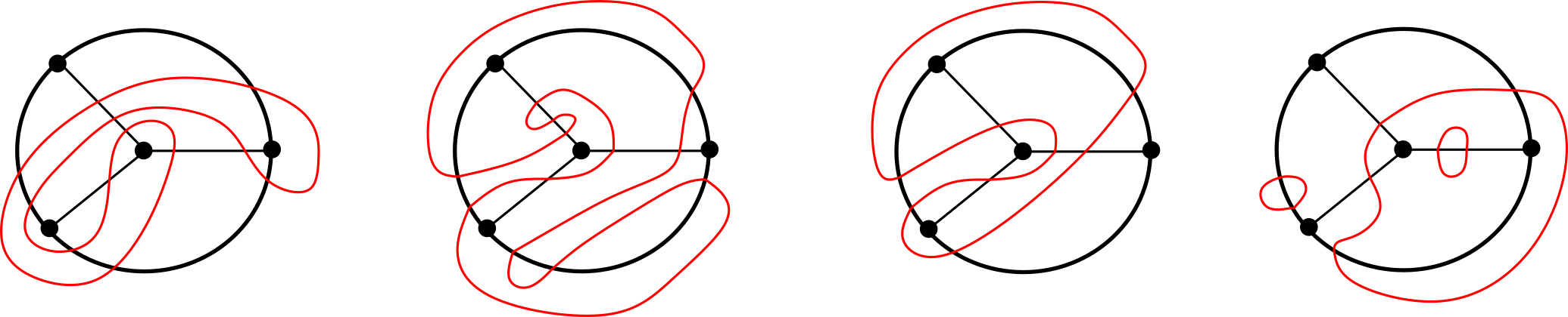
Figure 5. Pulling back a simple closed curve $\gamma$ (red) under a Schottky map $f$ corresponding to the tetrahedral Tischler graph $T$ (black). Starting on the left with a minimal curve $\gamma$ of complexity $\gamma\cdot T=12$, the next picture shows its preimage $\gamma_{1}^{\prime}=f^{-1}(\gamma)$, a simple closed curve with the same intersections, but $\gamma_{1}^{\prime}\cdot T=8$. The third picture shows a minimal curve $\gamma_{1}$ homotopic to $\gamma_{1}^{\prime}$, and the last picture shows the three components of its preimage $\gamma_{2}^{1}\cup\gamma_{2}^{2}\cup\gamma_{2}^{3}=f^{-1}(\gamma_{1})$, where $\gamma_{2}^{1}$ is minimal with $\gamma_{2}^{1}\cdot T=4$, and $\gamma_{2}^{2}$ and $\gamma_{2}^{3}$ are peripheral. The preimage $f^{-1}(\gamma_{2}^{1})$ (not depicted) is a simple closed curve $\gamma_{3}$ homotopic to $\gamma_{2}^{1}$.

We should remark on one essential difference between the orientation-preserving and orientation-reversing cases. In the orientation-preserving version of Lemma 5.8, strict inequality always holds if $\gamma$ intersects an edge of $T$ more than once [Hlu19]. As a consequence, a critically fixed rational maps $f$ always has a global curve attractor $\mathcal{A}(f)$, which is a finite set of homotopy classes of simple closed curves in $\mathbb{\hat{C}}\setminus P_{f}$ such that for every simple closed curve $\gamma\subset\mathbb{\hat{C}}\setminus P_{f}$ there exists $N$ such that for all $n\geq N$, all components of $f^{-n}(\gamma)$ are contained in $\mathcal{A}(f)$. For context, see Pilgrim’s paper [Pil12], where the question of the existence of global curve attractors for post-critically finite rational map was initiated.

Figure 6 gives an example of a Schottky map $f_{T}$ and a pair of minimal simple closed curves $\gamma_{1},\gamma_{2}$ in $S^{2}\setminus P_{f}$ which are pull-backs of each other up to homotopy in $S^{2}\setminus P_{f}$, and which both intersect an edge of $T$ twice. We will see that the topological Tischler graph $T$ in this example is unobstructed, so that the Schottky map $f_{T}$ is actually equivalent to an anti-rational map. This example shows that the proof of the existence of a global curve attractor in the orientation-preserving case does not carry over to the orientation-reversing case. Similarly, the recent proof of the existence of a global curve attractor in the polynomial case in [BLMW19] uses essentially polynomial tools, in particular Hubbard trees, so that the question of the existence of global curve attractors for post-critically finite anti-rational maps remains open.

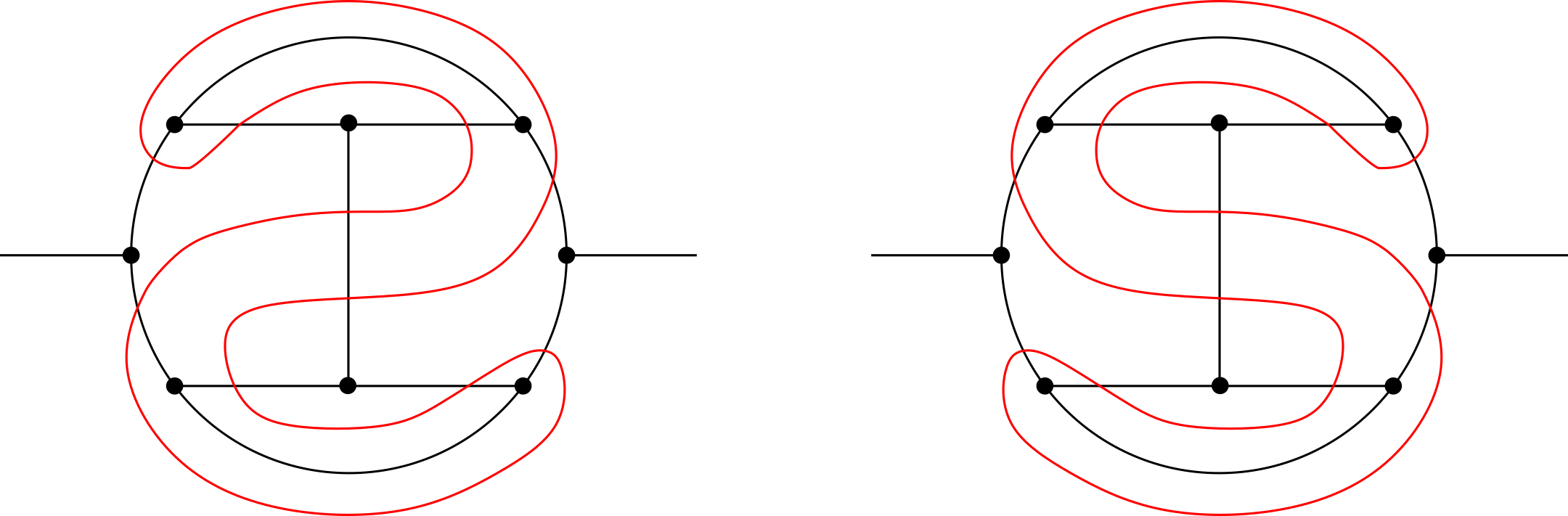
Figure 6. Example of a Tischler graph $T$ (black) and a pair of minimal simple closed curves $\gamma_{1}$ and $\gamma_{2}$ (red) with double edge intersections which are pull-backs of each other (up to homotopy) under the corresponding topological Schottky map. The edge segments of $T$ on the left and right are supposed to continue and join at $\infty$.

Theorem 5.9.

Let $T=(P,E)$ be a topological Tischler graph and $f=f_{T}$ be an associated Schottky map. Then one of the following mutually exclusive cases occurs:

$\bm{T}$ is obstructed:

There is a pair of distinct faces $A$ and $B$ of $T$ sharing two distinct edges $a,b\in\partial A\cap\partial B$. In this case, the map $f$ has a Levy cycle given by a simple closed curve $\gamma$ which intersects the Tischler graph exactly twice, once in $a$ and once in $b$. In particular, $f$ is not equivalent to an anti-rational map.

$\bm{T}$ is unobstructed:

For any two distinct faces $A$ and $B$, there is at most one edge in $\partial A\cap\partial B$. In this case, $f$ is combinatorially equivalent to an anti-rational map, unique up to Möbius conjugacy.

Remark.

Another way to phrase the condition on $T$ is to say that $T$ is obstructed if and only if the dual graph has a loop of length 2.

Proof.

If $T$ has $\leq 2$ vertices, we already know that $f_{T}$ is equivalent to $g(z)=\bar{z}^{d}$, and that any two faces $A$ and $B$ of $T$ share at most one edge, so for the rest of the proof we will assume that $T$ has $\geq 3$ vertices. In this case, the associated orbifold is hyperbolic, and by the orientation-reversing Thurston theorem we know that $f$ is equivalent to an anti-rational map if and only if $f$ does not have an obstruction, and that the equivalent anti-rational map is unique up to Möbius conjugacy.

We will start with the easy part. Assume that $T$ has a pair of faces $A$ and $B$ sharing two edges $a$ and $b$, and let $\gamma$ be a simple closed curve as described. First of all, we claim that $\gamma$ is non-peripheral. Let $U$ be a component of $S^{2}\setminus\gamma$. Since $a$ and $b$ are distinct edges, $U$ must contain some vertex $p\in\partial A$. If this is the only vertex of the Tischler graph contained in $U$, then we also have $p\in\partial B$, and then $a$ and $b$ must be edges incident with $p$. This would imply that $p$ has degree 2, but by assumption all vertices in Tischler graphs have degree $\geq 3$. This shows that each connected components of $S^{2}\setminus\gamma$ contains at least two vertices, and since the vertices are the post-critical points of $f$, we conclude that $\gamma$ is non-peripheral. If we denote the intersection points of $\gamma$ with $a$ and $b$ by $z$ and $w$, then $f^{-1}(\gamma)\cap A$ is a simple curve in $A$ joining $z$ to $w$, and $f^{-1}(\gamma)\cap B$ is a simple curve in $B$ joining $z$ to $w$. This shows that the union of those is a simple closed curve $\gamma^{\prime}$ which again intersects the Tischler graph exactly at $z$ and $w$, so $\gamma^{\prime}$ is homotopic to $\gamma$ in $S^{2}\setminus P$. Furthermore, the degree of $f$ on both $A$ and $B$ is $1$, so the degree of $f$ on $\gamma^{\prime}$ is 1, and $\gamma$ is a Levy cycle.

Now assume that $f$ has an obstruction $\Gamma$. Since the Thurston matrix only depends on the homotopy classes of the curves in $S^{2}\setminus P_{f}$, we may assume that the curves in $\Gamma$ are minimal. By Lemma 3.4, we may further assume that $\Gamma$ is an irreducible obstruction, so that the associated matrix $A=A_{f,\Gamma}$ is irreducible. Just as in the statement of Thurston’s theorem, we label the connected components of $f^{-1}(\gamma_{k})$ which are homotopic to $\gamma_{j}$ in $S^{2}\setminus P$ by $\gamma_{j,k,\alpha}$, and we let $d_{j,k,\alpha}$ be the degree of $f$ on $\gamma_{j,k,\alpha}$. From Lemma 5.8, we get that

$$\sum_{j,\alpha}\gamma_{j,k,\alpha}\cdot T\leq\gamma_{k}\cdot T.$$

In particular, this shows that $\gamma_{j}\cdot T\leq\gamma_{k}\cdot T$ whenever $f^{-1}(\gamma_{k})$ has a component homotopic to $\gamma_{j}$, so that the complexity $\kappa_{j}=\gamma_{j}\cdot T$ is non-increasing along the edges in the digraph associated to $A$. Since $A$ is irreducible, this digraph is strongly connected, so that $\kappa_{j}=\kappa$ is constant, independent of $j$. Again from Lemma 5.8 we conclude that there is only one non-peripheral connected component of $f^{-1}(\gamma_{k})$, minimal and homotopic to some $\gamma_{j}$, with all other components disjoint from $T$. This means that the associated digraph of $A$ has only one edge emanating from every $\gamma_{k}\in\Gamma$. A strongly connected digraph with this property has to be a cycle. Permuting the indices if necessary, this means that the associated Thurston linear map is given by $L(\gamma_{k})=\frac{1}{d_{k,k-1}}\gamma_{k-1}$. Here we omit the index $\alpha$ because $f^{-1}(\gamma_{k})$ has only one non-peripheral component, and we also understand indices modulo $n$, so that $\gamma_{n}=\gamma_{0}$. The associated matrix is then in cyclic normal form, and the Perron-Frobenius eigenvalue of $L$ is $\lambda=\prod_{k=1}^{n}\frac{1}{d_{k,k-1}}$. Since $\Gamma$ is an obstruction, we conclude that $\lambda=1$, and $d_{k,k-1}=1$ for $k=1,\ldots,n$, so that $\Gamma=\{\gamma_{1},\ldots,\gamma_{n}\}$ is a Levy cycle.

Now let $\gamma_{0}^{\prime}$ be the unique component of $f^{-1}(\gamma_{1})$ homotopic to $\gamma_{0}$. Then $f$ maps $\gamma_{0}^{\prime}$ one-to-one onto $\gamma_{1}$, and $\#(\gamma_{1}\cap T)=\gamma_{1}\cdot T=\gamma_{0}^{\prime}\cdot T=\#(\gamma_{0}^{\prime}\cap T)=\kappa$. Since $f$ is the identity on $T$, this implies that $\gamma_{1}\cap T=\gamma_{0}^{\prime}\cap T$. Let $A_{1},\ldots,A_{r}$ be the distinct faces of $T$ which intersect $\gamma_{1}$. Then $f^{-1}(\gamma_{1})\cap A_{k}$ consists of line segments connecting the intersection points $\gamma_{1}\cap\partial A_{k}$ inside $A_{k}$, so that $f^{-1}(\gamma_{1})\cap A_{k}=\gamma_{0}^{\prime}\cap A_{k}$. (All the other connected components of $f^{-1}(\gamma_{1})$ are contained in faces disjoint from $\gamma_{1}$.) So every point in $\gamma_{1}\cap A_{1}$ has exactly one preimage in $\gamma_{0}^{\prime}\cap A_{k}$ for $k=2,\ldots,r$. Since the degree of $f$ on $\gamma_{0}^{\prime}$ is 1, we must have $r=2$, so any edge crossed by $\gamma_{1}$ is a common edge between $A_{1}$ and $A_{2}$. By minimality of $\gamma_{1}$ (or, alternatively, by the fact that it is non-peripheral), it has to cross at least two distinct edges, so $\partial A_{1}$ and $\partial A_{2}$ share two distinct edges. ∎

In order to have a one-to-one correspondence between equivalence classes of unobstructed topological Tischler graphs and Möbius equivalence classes of anti-rational maps, we have to show that equivalence of Schottky maps implies equivalence of the corresponding graphs. This comes down to showing that for a Schottky map $f_{T}$, a “Tischler graph up to isotopy” is actually isotopic to $T$. For the following, an essential arc in $(S^{2},P)$ is an open simple arc in $S^{2}\setminus P$ with distinct endpoints, both in $P$. Homotopy and isotopy of arcs is always considered within the family of essential arcs, i.e., with endpoints in $P$ fixed, and the open arcs in $S^{2}\setminus P$. If $f$ is a Thurston or anti-Thurston map of degree $d$, and if $\gamma$ is an essential arc in $(S^{2},P_{f})$, its preimage $f^{-1}(\gamma)$ consists of $d$ disjoint arcs, not necessarily essential, each one of which is mapped homeomorphically onto $\gamma$. (We consider $\gamma$ as an open arc, so some of these preimages may have common endpoints.) An essential arc is invariant (with respect to $f$) if one of these preimages is homotopic to $\gamma$. An arc system $\Gamma$ is a finite collection of disjoint essential arcs which are not homotopic to each other. Examples of invariant essential arcs are the edges in the Tischler graph, and the Tischler graph is an example of an arc system. The following definition mimics the one for simple closed curves.

Definition 5.10.

The complexity of an essential arc $\gamma$ is the intersection number $\gamma\cdot T$, defined as the minimal number of intersections of $\gamma^{\prime}$ with $T$ over all $\gamma^{\prime}$ homotopic to $\gamma$. The complexity of an arc system $\Gamma$ is the intersection number $\Gamma\cdot T$, defined as the minimal number of intersections of $\Gamma^{\prime}$ with $T$, over all isotopic arc systems $\Gamma^{\prime}$. We say that an essential arc $\gamma$ or an arc system $\Gamma$ is minimal if they realize this intersection number.

Remark.

Since we consider arcs to be open, we do not count the endpoints in $P$ as intersection points for either arc systems or arcs. E.g., $\Gamma\cdot\Gamma=0$ for all arc systems, since we can isotope every arc to a “parallel”, slightly displaced disjoint arc.

Lemma 5.11.

Let $T=(P,E)$ be an unobstructed topological Tischler graph and $f=f_{T}$ an associated Schottky map. Let $\Gamma$ be an arc system consisting of invariant essential arcs. Then $\Gamma$ is ambient isotopic to a subgraph of $T$.

Remark.

Ambient isotopy means that the isotopy on the graphs extends to an isotopy of the sphere, fixing $P$ pointwise.

Proof.

We will first show that any invariant essential arc $\gamma$ is homotopic to an edge of $T$. We may assume that $\gamma$ is minimal, and we denote the endpoints of $\gamma$ by $p$ and $q$. Let $\gamma^{\prime}$ be a component of $f^{-1}(\gamma)$ homotopic to $\gamma$. By minimality of $\gamma$ and the same argument as in 5.8, $\gamma^{\prime}\cap T=\gamma\cap T=\kappa$.

We associate to $\gamma$ the sequence $(A_{0},z_{1},A_{1},z_{2}\ldots,z_{\kappa},A_{\kappa})$ of consecutive (not necessarily distinct) faces and edge intersections $z_{j}\in e_{j}$, and we denote the segments of $\gamma$ contained in those faces by $\gamma_{0},\ldots,\gamma_{\kappa}$. By minimality we always have $e_{j}\neq e_{j+1}$ (because consecutive intersections of the same edge can be removed by homotopy), and we also know that $e_{1}$ is not incident to $p$, and $e_{\kappa}$ is not incident to $q$ (for the same reason.) For $\gamma^{\prime}$ we will use the same notation, with primes on everything. We know that $\{z_{1},\ldots,z_{\kappa}\}=\{z_{1}^{\prime},\ldots z_{\kappa}^{\prime}\}$ holds as set equality, but not necessarily as ordered tuples.

If $\kappa=0$, then $\gamma$ is contained in $A=A_{0}$, so as a preimage, $\gamma^{\prime}$ has to be contained in a different face $B$. Then $\eta=\{p,q\}\cup\gamma\cup\gamma^{\prime}$ is a Jordan curve containing two different vertices of $T$, and by the assumption that $\gamma$ and $\gamma^{\prime}$ are homotopic, $\eta$ can not separate $P$, so one of the components of $S^{2}\setminus\eta$ must be disjoint from $P$. However, since $\gamma$ and $\gamma^{\prime}$ are in different faces, that component must contain an edge $e$ of $T$ from $p$ to $q$, which is then homotopic to both $\gamma$ and $\gamma^{\prime}$.

Figure 7. Illustration of the $\kappa=1$ case

If $\kappa=1$, then $\gamma$ and $\gamma^{\prime}$ cross only one edge $e_{1}$ between $A_{0}$ and $A_{1}$ at $z_{1}$, and so $\gamma^{\prime}$ is the image of $\gamma$ under the branch of $f^{-1}$ fixing $e_{1}$, defined in $A_{0}\cup A_{1}$, and locally (near $z_{1}$) mapping $A_{0}$ to $A_{1}$ and vice versa. This shows that $\gamma_{0}$ and $\gamma_{1}^{\prime}$ are both simple paths from $p$ to $z_{1}$, in different faces $A_{0}$ and $A_{1}$ of $T$. Then $\eta=\{p,z_{1}\}\cup\gamma_{0}\cup\gamma^{\prime}_{1}\subset\gamma\cup\gamma^{\prime}$ is a Jordan curve, and since $z_{1}$ is on an edge $e_{1}$ not incident with $p$, the endpoints of $e_{1}$ are in different components of $S^{2}\setminus\eta$. This shows that $\gamma$ and $\gamma^{\prime}$ are two halves of a figure eight curve, with at least two points of $P$ contained in the interior of each of the bounded complementary components. Since $\gamma$ and $\gamma^{\prime}$ are not homotopic as arcs in the sphere with the two endpoints and the four interior points marked, depicted in Figure 7, they are not homotopic in $(S^{2},P)$ either.

If $\kappa\geq 2$, we know that $A_{0},A_{1}$, and $A_{2}$ are three distinct faces of $T$, since we assumed that $T$ is not obstructed. Then $\gamma_{1}$ has one preimage each in $A_{0}$ and $A_{2}$, both of them with endpoints in $T$, so both of them part of $\gamma^{\prime}$. However, this contradicts the fact that $f$ maps $\gamma^{\prime}$ one-to-one onto $\gamma$.

Now if $\Gamma$ is an arc system consisting of invariant essential arcs, we may again assume that $\Gamma$ is minimal. Then the same arguments given above apply to show that $\gamma\cap T=\emptyset$ for all $\gamma\in\Gamma$. This means that all the arcs of $\Gamma$ are contained in faces of $T$, and by the first part we know that they are homotopic to corresponding edges. This easily implies that $\Gamma$ is ambient isotopic to the corresponding subgraph of $T$. ∎

Remark.

This result should still hold without the assumption that $T$ is unobstructed. However, the $\kappa\geq 2$ case gets more complicated, and since we mainly want to apply this to critically fixed anti-rational maps, we only need it for unobstructed graphs.

Corollary 5.12.

Let $T=(P,E)$ and $T^{\prime}=(P^{\prime},E^{\prime})$ be unobstructed topological Tischler graphs, and assume that associated Schottky maps $f=f_{T}$ and $f^{\prime}=f_{T^{\prime}}$ are equivalent. Then their topological Tischler graphs $T$ and $T^{\prime}$ are equivalent.

Proof.

If $\phi\circ f=f^{\prime}\circ\psi$ is a combinatorial equivalence, then $\Gamma=\phi(T)$ is an $f^{\prime}$-invariant arc system, so by 5.11 it is ambient isotopic to a subgraph of $T^{\prime}$. Since $\Gamma$ and $T^{\prime}$ have the same number of arcs (edges), this shows that $\Gamma$ is ambient isotopic to $T^{\prime}$, so it is in particular equivalent. ∎

Combining our results, we can now precisely state the one-to-one correspondence between critically fixed anti-rational maps and unobstructed topological Tischler graphs. For $d\geq 2$, let $\mathcal{F}_{d}$ be the set of Möbius equivalence classes of critically fixed anti-rational maps of degree $d$, and let $\mathcal{G}_{d}$ be the set of equivalence classes of unobstructed topological Tischler graphs with $d+1$ faces. Given $[T]\in\mathcal{G}_{d}$, there exists an associated Schottky map $f_{T}$, and a combinatorially equivalent anti-rational map $f$. By Lemma 5.5 and Theorem 5.9, different choices of representatives $T$ of the equivalence class in $\mathcal{G}_{d}$, and different choices of the Schottky map $f_{T}$ always yield a unique equivalence class $[f]$, so that we have a well-defined map $\Psi:\mathcal{G}_{d}\to\mathcal{F}_{d}$. Conversely, if $f$ and $g$ are two Möbius conjugate critically fixed anti-rational functions, then their Tischler graphs $T_{f}$ and $T_{g}$ are equivalent, since they are images of each other under Möbius transformations. This shows that $f\mapsto T_{f}$ induces a well-defined map $\Theta:\mathcal{F}_{d}\to\mathcal{G}_{d}$.

Theorem 5.13.

There is a one-to-one correspondence between equivalence classes of unobstructed topological Tischler graphs and Möbius conjugacy classes of critically fixed anti-rational maps. More precisely, for every $d\geq 2$, the map $\Psi:\mathcal{G}_{d}\to\mathcal{F}_{d}$ is a bijection with inverse $\Psi^{-1}=\Theta$.

Proof.

Corollary 5.12 shows that $\Psi$ is injective, and Theorem 5.6 shows that $\Psi\circ\Theta=\operatorname{id}$. This implies both that $\Psi$ is surjective, and that $\Psi^{-1}=\Theta$. ∎

A very useful consequence is that anti-rational maps inherit any symmetries of its topological Tischler graph. The group of symmetries of a plane graph $T$ is the group $\Gamma$ of Möbius or anti-Möbius transformations $\theta$ with $\theta(T)=T$. Similarly, the group of symmetries of a map $f:\mathbb{\hat{C}}\to\mathbb{\hat{C}}$ is the group $\Gamma$ of Möbius or anti-Möbius transformations $\theta$ which commute with $f$, i.e., for which $f\circ\theta=\theta\circ f$. We say that $f$ is $\Gamma$-symmetric if its symmetry group contains $\Gamma$. In the special case where the symmetry group contains complex conjugation $\iota(z)=\bar{z}$, we say that the plane graph $T$ or the map $f$ is $\mathbb{R}$-symmetric.

Theorem 5.14.

Let $T\subset\mathbb{\hat{C}}$ be an unobstructed topological Tischler graph with $\geq 3$ vertices, and let $\Gamma$ be its symmetry group. Then there exists a $\Gamma$-symmetric anti-rational map $f$ corresponding to $T$. More precisely, there exists a $\Gamma$-symmetric Schottky map $f_{T}$, and if $\phi\circ f_{T}=\psi\circ f$ is a combinatorial equivalence to an anti-rational map $f$ with the property that $\phi$ and $\psi$ fix three different vertices of $T$, then $f$ is $\Gamma$-symmetric.

Remark.

Obviously, if $f$ is any anti-rational map corresponding to $T$, without requiring that the combinatorial equivalence fixes three vertices, it is $\Gamma^{\prime}$-symmetric, where $\Gamma^{\prime}$ is conjugate to $\Gamma$. If $T$ has only two vertices, then the theorem is not correct, but the only examples in that case are conjugate to $f(z)=\bar{z}^{d}$.

Proof.

Since $\Gamma$ permutes the $\geq 3$ vertices of $T$, it has to be a finite group, containing only reflections in lines and circles, and elliptic Möbius transformations of finite order. With this, it is not hard to show that one can find a $\Gamma$-symmetric Schottky map $f_{T}$. If we have a combinatorial equivalence $\phi\circ f_{T}=f\circ\psi$ where $\phi$ and $\psi$ fix three vertices of $T$, then by conjugation we may assume that these are 0, 1, and $\infty$. With this, the claim of the theorem follows directly from Corollary 3.10. ∎

6. Critically fixed anti-polynomials

In this section we are going to apply our methods to the special case of critically fixed anti-polynomials, providing an alternative approach to the results in [Gey08] and [LMM21], as well as generalizing them by allowing multiple critical points. In the anti-polynomial case, the topological Tischler graph is special, because the point at $\infty$ is a critical point of multiplicity $d-1$, where $d$ is the degree of the anti-polynomial. For convenience, in this section we will implicitly always work with a marked sphere $(S^{2},\infty)$, with a designated point at infinity, and we will write $\mathbb{R}^{2}=S^{2}\setminus\{\infty\}$. All conjugacies and combinatorial equivalences here are supposed to fix $\infty$, mapping $\mathbb{R}^{2}$ to $\mathbb{R}^{2}$.

Definition 6.1.

A plane graph $\hat{T}\subset S^{2}$ is an anti-polynomial topological Tischler graph if it is a topological Tischler graph with $n\geq 3$ faces, where $\infty$ is a vertex of degree $n$.

Remark.

Note that the condition that the faces are Jordan domains implies that the $n$ faces at $\infty$ are all distinct, so the condition implies that every face has $\infty$ on the boundary.

Definition 6.2.

We say that $T\subset\mathbb{R}^{2}$ is an unbounded plane tree if $T$ is closed (as a subset of $\mathbb{R}^{2}$) and homeomorphic to a plane tree without vertices of degree 2, and with all its leaves removed. A topological Tischler tree is an unbounded plane tree with $\geq 3$ unbounded edges.

Remark.

Note that the condition that $T$ is closed means that “leaf edges” of $T$ necessarily have to be unbounded. An unbounded plane tree should be thought of as a tree with all its leaves at $\infty$. Obviously, the one-point compactification $\hat{T}$ of $T$ will not be a tree anymore. An equivalent model for unbounded plane trees which is easier to draw and which we will use in illustrating our examples is to identify $\mathbb{R}^{2}$ with the open unit disk $D^{2}$ and to consider trees $\overline{T}$ in the closed unit disk $\overline{D^{2}}=D^{2}\cup S^{1}$ such that $\overline{T}\setminus D^{2}=\overline{T}\cap S^{1}$ consists exactly of the leaves of $\overline{T}$. In this case, $T=\overline{T}\cap D^{2}=T\setminus S^{1}$.

Theorem 6.3.

Let $\hat{T}$ be an anti-polynomial topological Tischler graph. Then $\hat{T}$ is unobstructed, and $T=\hat{T}\cap\mathbb{R}^{2}$ is a topological Tischler tree. Conversely, for every topological Tischler tree $T$, we have that $\hat{T}=T\cup\{\infty\}$ is an anti-polynomial topological Tischler graph.

Proof.

Assume that $\hat{T}$ is obstructed, and let $A\neq B$ be two faces sharing two distinct edges $a,b\in\partial A\cap\partial B$. Let $\gamma$ be a simple closed curve in $S^{2}\setminus P$ intersecting $\hat{T}$ exactly twice, once each in $a$ and $b$, and let $U$ and $V$ be the components of $S^{2}\setminus\gamma$, with $\infty\in U$. Since $\gamma$ does not intersect any faces other than $A$ and $B$, and since every face has $\infty$ on its boundary, we must have $C\subset U$ for all faces $C\notin\{A,B\}$. This shows that all vertices of the Tischler graph are contained in $U$, contradicting the fact that both components of $\partial A\setminus\gamma$ must have vertices of $T$, since $a$ and $b$ were assumed to be different edges.

Now $T=\hat{T}\setminus\{\infty\}$ can not contain any loops, since every face of $\hat{T}$ has $\infty$ on its boundary. If $A_{1},\ldots,A_{n}$ denotes the faces of $\hat{T}$ in cyclic order around $\infty$, and if we define $\hat{C}_{k}=\partial A_{k}$ and $C_{k}=\hat{C}_{k}\setminus\{\infty\}$, then $T=\bigcup_{k=1}^{n}C_{k}$. Since $C_{k}$ is a Jordan curve in $S^{2}$ with only the one point at $\infty$ removed, it is still connected, and since $C_{k}$ and $C_{k-1}$ have an unbounded edge in common, we have that $C_{k}\cap C_{k-1}\neq\emptyset$ (where we use indices modulo $n$), so that $T$ is connected, and hence an unbounded tree. Since $\infty$ has degree $\geq 3$ for $\hat{T}$, we have that $T$ has $\geq 3$ unbounded edges, and thus it is a topological Tischler graph.

For the converse, note that the faces of $T$ (in $\mathbb{R}^{2}$) agree with the faces of $\hat{T}$, and since $T$ is a tree with $\geq 3$ unbounded edges, every face of $T$ is bounded by a Jordan curve in $S^{2}$. The degree of $\infty$ in $\hat{T}$ is again the number of unbounded edges, so it is $\geq 3$, and thus $\hat{T}$ is an anti-polynomial topological Tischler graph. ∎

Remark.

An obvious consequence of Theorem 6.3 is that there is a one-to-one correspondence between anti-polynomial topological Tischler graphs $\hat{T}$ and topological Tischler trees $T$, given by $\hat{T}=T\cup\{\infty\}$.

Theorem 6.4.

Let $T$ be a topological Tischler tree, and $f_{T}$ an associated Schottky map. Then $f_{T}$ is combinatorially equivalent to a critically fixed anti-polynomial, unique up to affine conjugacy.

Proof.

This follows by combining Theorem 5.9 with Theorem 6.3. ∎

We define the Tischler tree of a critically fixed anti-polynomial $f$ as the Tischler graph without the vertex at $\infty$. Every unbounded edge is the concatenation of one internal ray and one external ray landing at a common repelling fixed point in the Julia set. It is easy to see that the bounded part of the Tischler tree, i.e., the Tischler tree without all the unbounded edges, is exactly the Hubbard tree of the anti-polynomial.

7. Examples and Applications

In this section we first list critically fixed maps of small degrees, and then give a few interesting examples and applications to mappings of higher degrees. All classifications and statements of uniqueness are up to Möbius conjugacy, and in the case of anti-polynomials up to affine conjugacy. We have not spent much effort to calculate explicit maps, except for some of the straightforward easy cases.

To any anti-rational map of degree $d\geq 2$ we will associate its branching data $(m_{1},\ldots,m_{r})$ where $m_{1}\geq\ldots\geq m_{r}\geq 1$ are the multiplicities of the distinct critical points $c_{1},\ldots,c_{r}$. We then have $1\leq m_{k}\leq d-1$, and $\sum_{k=1}^{r}m_{k}=2d-2$. A critically fixed anti-rational map is Möbius conjugate to an anti-polynomial if and only if $m_{1}=d-1$.

Throughout this section, Tischler graphs and Tischler trees have been drawn to realize all possible symmetries. In particular, if possible they have been drawn $\mathbb{R}$-symmetrically, which means that the corresponding anti-polynomial or anti-rational maps can be chosen to have real coefficients. If furthermore all vertices can be realized on the real line, this has been done, too. In that case, the corresponding anti-polynomial or anti-rational map is the complex conjugate of a critically fixed polynomial or rational map.

7.1. Critically fixed anti-polynomials of low degrees

For anti-polynomials of degree $d\geq 2$ we omit the critical point at $\infty$ in our branching data, so these will be given by $(m_{1},\ldots,m_{r})$ where $m_{1}\geq m_{2}\geq\ldots\geq m_{r}$ are the multiplicities of the finite critical points $c_{1},\ldots,c_{r}$ with $\sum_{k=1}^{r}=d-1$. Instead of organizing the list by degree, it is easier to organize by the number $r$ of distinct finite critical points, which is also the number of vertices in the Tischler tree and the corresponding Hubbard tree. For $r\leq 2$ it is not hard to list all possible critically fixed anti-polynomials. For $r\geq 3$ we list all possible Tischler trees, with some remarks on the corresponding anti-polynomials. The figures illustrating the Tischler trees all have a dashed “circle at infinity” and are labeled by their branching data. The bounded edges which make up the Hubbard tree are drawn a little thicker for emphasis. A few of these anti-polynomials have been explicitly calculated using ad-hoc methods and computer algebra in [BL04], but with our combinatorial description it should be easier to systematically find them numerically.

7.1.1. $r=1$

In this case, the only possible branching data is $(m)$ with degree $d=m+1$, and the unique corresponding critically fixed anti-polynomial is $f(z)=\bar{z}^{d}$.

Figure 8. Tischler trees with one vertex up to degree 5.

7.1.2. $r=2$

We can always normalize these maps to have critical points $p_{0}=0$ and $p_{1}=1$, with branching data $(m_{0},m_{1})$ and degree $d=m_{0}+m_{1}+1$. For every such pair of multiplicities there is a unique associated Tischler tree, with vertex degrees $m_{0}+2$ at $p_{0}$ and $m_{1}+2$ at $p_{1}$, one edge from $p_{0}$ to $p_{1}$, and all other edges unbounded. The corresponding anti-polynomials are complex conjugates of critically fixed polynomials $f_{m_{0},m_{1}}$ with the same critical points, given by the regularized incomplete beta function

$$f_{m_{0},m_{1}}(z)=\frac{B(z;\,m_{0}+1,m_{1}+1)}{B(m_{0}+1,m_{1}+1)}=\frac{(m_{0}+m_{1}+1)!}{m_{0}!m_{1}!}\int_{0}^{z}\zeta^{m_{0}}(1-\zeta)^{m_{1}},\,d\zeta.$$

The first few ones, up to degree $d=5$, are given explicitly as

$$f_{1,1}(z) =3z^{2}-2z^{3} f_{2,1}(z) =4z^{3}-3z^{4}$$

$$f_{3,1}(z) =5z^{4}-4z^{5} f_{2,2}(z) =10z^{3}-15z^{4}+6z^{5}$$

Figure 9. Tischler trees with two vertices up to degree 5.

7.1.3. $r=3$

In this case we have branching data $(m_{1},m_{2},m_{3})$ with $d=m_{1}+m_{2}+m_{3}+1$. There is only one possible Hubbard tree as a subset of the plane, with one vertex of degree 2, and two vertices of degree 1. However, unless $m_{1}=m_{2}=m_{3}$, there are different ways to distribute these multiplicities on the Hubbard tree, giving inequivalent maps. Furthermore, in general there are different choices for the “turn angle” at the vertex of degree 2. The different inequivalent Tischler trees encode all these different choices.

For branch data $(1,1,1)$ there is a unique associated Tischler tree, and an associated anti-polynomial $f$ of degree 4 with real coefficients, and one real and two complex conjugate critical points.

For branch data $(2,1,1)$ there are four associated Tischler trees, and correspondingly four different critically fixed anti-polynomials. Two of them have the double critical point at the vertex of degree 2 in the Hubbard tree. For one of them, the two edges in the Hubbard tree are not adjacent in the cyclic order in the Tischler tree, i.e., they are separated by unbounded edges. This corresponds to an angle of $180^{\circ}$ between them in the angled Hubbard tree. In the other one, they are adjacent, corresponding to a $90^{\circ}$ angle between them. The two other Tischler trees have the double critical point as a leaf in the Hubbard tree. This means that the angle at the vertex of degree $2$ in the Hubbard tree is $120^{\circ}$. However, because the Hubbard tree is not symmetric with respect to interchanging the leaves (since one is a simple and the other a double critical point), the two different orientations of this angle give inequivalent Tischler trees. These are the first examples in this list which can not be realized as an anti-polynomials with real coefficients.

Figure 10. Tischler trees with three vertices up to degree 5. The first three are $\mathbb{R}$-symmetric, the last two are mirror images under complex conjugation.

7.1.4. $r=4$

For branch data $(1,1,1,1)$ we have four different Tischler trees. One of them has a Hubbard tree with a vertex of degree 3 and 3 leaves, the other three have two Hubbard vertices of degree 2 and 2 leaves, and only differ in their turning angles at the degree 2 leaves. In this case, the Hubbard tree is symmetric with respect to switching the leaves, but the two trees with opposite $120^{\circ}$ degree turns are not equivalent by an orientation-preserving homeomorphism, which again leads to two different Möbius conjugacy classes which are anti-Möbius conjugate.

Figure 11. Tischler trees with four vertices up to degree 5. The first two are $\mathbb{R}$-symmetric, the last two are mirror images under complex conjugation.

7.2. Critically fixed non-polynomial maps of low degrees

In order to list the unobstructed Tischler graphs for anti-rational maps of degree $d$ which are not equivalent to polynomials, we have to consider branching data $(m_{1},\ldots,m_{r})$ with $d-2\geq m_{1}\geq m_{2}\geq\ldots\geq m_{r}\geq 1$ and $\sum_{k=1}^{r}m_{k}=2d-2$, for $d\geq 3$. The following list all possible such graphs for degrees 3 and 4. Similar as for anti-polynomials, this combinatorial description should make it possible to calculate these maps numerically.

7.2.1. $d=3$

The only unobstructed topological Tischler graph here is the complete graph on 4 vertices. The corresponding map is the tetrahedral map

$$f(z)=\frac{3\bar{z}^{2}}{2\bar{z}^{3}+1}.$$

Figure 12. Unique unobstructed topological Tischler graph of degree $d=3$, corresponding to the tetrahedral map.

7.2.2. $d=4$

Figure 13 shows all the unobstructed topological Tischler graphs for degree 4 which do not come from anti-polynomials. Note that the first two graphs, with branching data $(2,2,2)$ and $(2,2,1,1)$, correspond to complex conjugates of critically fixed rational maps, since the graphs are $\mathbb{R}$-symmetric and have all critical points on the real line. Möbius conjugates of these two rational maps are explicitly calculated in [CGN⁺15, Section 11].

All but two of the graphs (the Z-shaped graphs with branching data $(2,2,1,1)$) are $\mathbb{R}$-symmetric, so they correspond to critically fixed anti-rational maps with real coefficients. The unique graph with branching data $(1,1,1,1,1,1)$ is a prism graph.

Figure 13. Non-polynomial unobstructed topological Tischler graphs for degree 4, labeled by branching data.

7.3. Maps with symmetries

If $\Gamma$ is a finite group of spherical isometries, then every element of $\Gamma$ commutes with the antipodal map $\tau(z)=-1/\bar{z}$, so $f$ is a rational map with $\Gamma$-symmetry if and only if $g=\tau\circ f$ is an anti-rational map with $\Gamma$-symmetry. This gives an explicit one-to-one correspondence between $\Gamma$-symmetric rational and anti-rational maps, under which critically fixed anti-rational map correspond to “critically antipodal” rational maps, i.e., rational maps which map each critical point to its antipode. Some of the references given in the following concern only rational maps, but the results and formulas obviously directly imply the corresponding results and formulas for anti-rational maps.

We have already encountered the tetrahedral map as the unique critically fixed anti-rational map with branching data $(1,1,1,1)$. In a slightly different normalization, this map arises without the need to use Thurston’s theorem in the following way: Draw a regular spherical tetrahedron, and in each face $A$, define $f$ to be the anti-conformal map from $A$ to its complement $\mathbb{\hat{C}}\setminus\overline{A}$, fixing the vertices. By symmetry, these conformal maps fit together along the edges, resulting in a critically fixed anti-rational map of degree 3 with 4 simple critical points and tetrahedral symmetry. The same construction can be carried out for all Platonic solids. In [DM89], these maps were calculated for the dodecahedron and icosahedron, and this and other methods are used to explicitly find all rational maps of degree $d\leq 30$ with icosahedral symmetry. (The authors remark that there is good evidence that these maps were already known to Felix Klein.) It turns out that all of these maps are post-critically finite, and indeed complex conjugates of critically fixed anti-rational maps. See [LLM22] for explicit formulas for the remaining Platonic solid, and pictures of the corresponding Julia sets.

In degree $d=31$, there is a non-trivial one-parameter family of rational maps with icosahedral symmetry, most of which are not post-critically finite. In [Cra14], Crass calculated two critically fixed anti-rational maps of degree 31 explicitly, and conjectured that these are the only such maps with simple critical points. The associated Tischler graphs are a “soccer ball” (truncated icosahedron) $T_{1}$, and a truncated dodecahedron $T_{2}$. It is well-known that the only polyhedra with 32 faces and icosahedral symmetry are those two and the icosidodecahedron $T_{3}$, which has 20 triangular faces and 12 pentagonal faces. However, while $T_{1}$ and $T_{2}$ have 60 vertices, each of degree 3, the icosidodecahedron has only 30 vertices, each of degree 4. Combining the classification of polyhedra with Theorems 5.13 and 5.14, we have the following, resolving Crass’s conjecture:

Theorem 7.1.

There are exactly three critically fixed anti-rational maps $f_{k}$, $k=1,2,3$, of degree $d=31$ with icosahedral symmetry, with associated Tischler graphs $T_{k}$. The maps $f_{1}$ and $f_{2}$ each have 60 simple critical points, the map $f_{3}$ has 30 double critical points.

This conjecture had been verified numerically by Crass, who continued his investigation in [Cra20] to numerically find all rational maps of degre 31 with icosahedral symmetry and periodic critical points. Obviously, analogues of Theorem 7.1 hold for any given degree $d$ and symmetry group $\Gamma$. In general, the $\Gamma$-symmetric critically fixed anti-rational maps are classified by $\Gamma$-symmetric polyhedra with $d+1$ faces.

References

- [BBY12] Sylvain Bonnot, Mark Braverman, and Michael Yampolsky, Thurston equivalence to a rational map is decidable, Mosc. Math. J. 12 (2012), no. 4, 747–763. MR 3076853
- [BCT14] Xavier Buff, Guizhen Cui, and Lei Tan, Teichmüller spaces and holomorphic dynamics, Handbook of Teichmüller Theory. Vol. IV, IRMA Lect. Math. Theor. Phys., vol. 19, Eur. Math. Soc., Zürich, 2014, pp. 717–756. MR 3289714
- [Bea91] Alan F. Beardon, Iteration of rational functions, Graduate Texts in Mathematics, vol. 132, Springer-Verlag, New York, 1991. MR 1128089
- [BL04] Daoud Bshouty and Abdallah Lyzzaik, On Crofoot-Sarason’s conjecture for harmonic polynomials, Comput. Methods Funct. Theory 4 (2004), no. 1, 35–41. MR 2081663
- [BLMW19] James Belk, Justin Lanier, Dan Margalit, and Rebecca R. Winarski, Recognizing topological polynomials by lifting trees, arXiv:1906.07680 [math] (2019).
- [BM17] Mario Bonk and Daniel Meyer, Expanding Thurston maps, Mathematical Surveys and Monographs, vol. 225, American Mathematical Society, Providence, RI, 2017. MR 3727134
- [CG93] Lennart Carleson and Theodore W. Gamelin, Complex dynamics, Universitext: Tracts in Mathematics, Springer-Verlag, New York, 1993. MR 1230383
- [CGN+15] Kristin Cordwell, Selina Gilbertson, Nicholas Nuechterlein, Kevin M. Pilgrim, and Samantha Pinella, On the classification of critically fixed rational maps, Conform. Geom. Dyn. 19 (2015), 51–94. MR 3323420
- [CHRS89] W. D. Crowe, R. Hasson, P. J. Rippon, and P. E. D. Strain-Clark, On the structure of the Mandelbar set, Nonlinearity 2 (1989), no. 4, 541–553. MR 1020441
- [Cra14] Scott Crass, Dynamics of a Soccer Ball, Experimental Mathematics 23 (2014), no. 3, 261–270.
- [Cra20] by same author, Critically-Finite Dynamics on the Icosahedron, Symmetry 12 (2020), no. 1, 177.
- [DH93] Adrien Douady and John H. Hubbard, A proof of Thurston’s topological characterization of rational functions, Acta Math. 171 (1993), no. 2, 263–297. MR 1251582
- [DM89] Peter Doyle and Curt McMullen, Solving the quintic by iteration, Acta Math. 163 (1989), no. 3-4, 151–180. MR 1032073
- [Gey08] Lukas Geyer, Sharp bounds for the valence of certain harmonic polynomials, Proc. Amer. Math. Soc. 136 (2008), no. 2, 549–555. MR 2358495
- [Hlu19] Mikhail Hlushchanka, Tischler graphs of critically fixed rational maps and their applications, arXiv:1904.04759 [math] (2019).
- [HP09] Peter Haïssinsky and Kevin M. Pilgrim, Coarse expanding conformal dynamics, Astérisque (2009), no. 325, viii+139 pp. (2010). MR 2662902
- [HS14] John Hamal Hubbard and Dierk Schleicher, Multicorns are not path connected, Frontiers in Complex Dynamics, Princeton Math. Ser., vol. 51, Princeton Univ. Press, Princeton, NJ, 2014, pp. 73–102. MR 3289907
- [Hub16] John Hamal Hubbard, Teichmüller theory and applications to geometry, topology, and dynamics. Vol. 2, Matrix Editions, Ithaca, NY, 2016. MR 3675959
- [KN06] Dmitry Khavinson and Genevra Neumann, On the number of zeros of certain rational harmonic functions, Proc. Amer. Math. Soc. 134 (2006), no. 4, 1077–1085. MR 2196041
- [KN08] by same author, From the fundamental theorem of algebra to astrophysics: A “harmonious” path, Notices Amer. Math. Soc. 55 (2008), no. 6, 666–675. MR 2431564
- [Lev85] Silvio Vieira Ferreira Levy, Critically finite rational maps, Ph.D. thesis, ProQuest LLC, Ann Arbor, MI, 1985. MR 2634168
- [LLM22] Russell Lodge, Yusheng Luo, and Sabyasachi Mukherjee, Circle packings, kissing reflection groups and critically fixed anti-rational maps, Forum Math. Sigma 10 (2022), Paper No. e3, 38. MR 4365080
- [LLMM19] Russell Lodge, Mikhail Lyubich, Sergei Merenkov, and Sabyasachi Mukherjee, On Dynamical Gaskets Generated by Rational Maps, Kleinian Groups, and Schwarz Reflections, arXiv:1912.13438 [math] (2019).
- [LMM21] Kirill Lazebnik, Nikolai G. Makarov, and Sabyasachi Mukherjee, Univalent polynomials and Hubbard trees, Trans. Amer. Math. Soc. 374 (2021), no. 7, 4839–4893. MR 4273178
- [Mil06] John Milnor, Dynamics in one complex variable, third ed., Annals of Mathematics Studies, vol. 160, Princeton University Press, Princeton, NJ, 2006. MR 2193309
- [MNS17] Sabyasachi Mukherjee, Shizuo Nakane, and Dierk Schleicher, On multicorns and unicorns II: Bifurcations in spaces of antiholomorphic polynomials, Ergodic Theory Dynam. Systems 37 (2017), no. 3, 859–899. MR 3628924
- [Nak93] Shizuo Nakane, Connectedness of the tricorn, Ergodic Theory Dynam. Systems 13 (1993), no. 2, 349–356. MR 1235477
- [NS03] Shizuo Nakane and Dierk Schleicher, On multicorns and unicorns. I. Antiholomorphic dynamics, hyperbolic components and real cubic polynomials, Internat. J. Bifur. Chaos Appl. Sci. Engrg. 13 (2003), no. 10, 2825–2844. MR 2020986
- [Par22] Insung Park, Levy and Thurston obstructions of finite subdivision rules, arXiv:2012.00243 [math] (2022).
- [Pil01] Kevin M. Pilgrim, Canonical Thurston obstructions, Adv. Math. 158 (2001), no. 2, 154–168. MR 1822682
- [Pil12] by same author, An algebraic formulation of Thurston’s characterization of rational functions, Ann. Fac. Sci. Toulouse Math. (6) 21 (2012), no. 5, 1033–1068. MR 3088266
- [PL98] Kevin M. Pilgrim and Tan Lei, Combining rational maps and controlling obstructions, Ergodic Theory Dynam. Systems 18 (1998), no. 1, 221–245. MR 1609463
- [Ste93] Norbert Steinmetz, Rational iteration, De Gruyter Studies in Mathematics, vol. 16, Walter de Gruyter & Co., Berlin, 1993. MR 1224235
- [Thu16] Dylan P. Thurston, From rubber bands to rational maps: A research report, Res. Math. Sci. 3 (2016), Paper No. 15, 49. MR 3500499
- [Thu19] by same author, Elastic graphs, Forum Math. Sigma 7 (2019), e24, 84. MR 3993808
- [Tis89] David Tischler, Critical points and values of complex polynomials, J. Complexity 5 (1989), no. 4, 438–456. MR 1028906