Understanding Anomaly Detection with Deep Invertible Networks through Hierarchies of Distributions and Features

Abstract

Deep generative networks trained via maximum likelihood on a natural image dataset like CIFAR10 often assign high likelihoods to images from datasets with different objects (e.g., SVHN). We refine previous investigations of this failure at anomaly detection for invertible generative networks and provide a clear explanation of it as a combination of model bias and domain prior: Convolutional networks learn similar low-level feature distributions when trained on any natural image dataset and these low-level features dominate the likelihood. Hence, when the discriminative features between inliers and outliers are on a high-level, e.g., object shapes, anomaly detection becomes particularly challenging. To remove the negative impact of model bias and domain prior on detecting high-level differences, we propose two methods, first, using the log likelihood ratios of two identical models, one trained on the in-distribution data (e.g., CIFAR10) and the other one on a more general distribution of images (e.g., 80 Million Tiny Images). We also derive a novel outlier loss for the in-distribution network on samples from the more general distribution to further improve the performance. Secondly, using a multi-scale model like Glow, we show that low-level features are mainly captured at early scales. Therefore, using only the likelihood contribution of the final scale performs remarkably well for detecting high-level feature differences of the out-of-distribution and the in-distribution. This method is especially useful if one does not have access to a suitable general distribution. Overall, our methods achieve strong anomaly detection performance in the unsupervised setting, and only slightly underperform state-of-the-art classifier-based methods in the supervised setting. Code can be found at https://github.com/boschresearch/hierarchical_anomaly_detection.

1 Introduction

One line of work for anomaly detection - to detect if a given input is from the same distribution as the training data - uses the likelihoods provided by generative models. Through likelihood maximization, they are trained to yield high likelihoods on the in-distribution inputs (a.k.a. inliers). After training, one may expect out-of-distribution inputs (a.k.a. outliers) to have lower likelihoods than the inliers. However, this is often not the case. For example, Nalisnick et al. [22] showed that generative models trained on CIFAR10 [14] assign higher likelihoods to SVHN [24] than to CIFAR10 images.

Several works have investigated a potential reason for this failure: The image likelihoods of deep generative networks can be well-predicted from simple factors. For example, the deep generative networks’ image likelihoods highly correlate with: the image encoding sizes from a lossless compressor such as PNG [32]; background statistics, e.g., the number of zeros in Fashion-MNIST/MNIST images [27]; smoothness and size of the background [16]. These factors do not directly correspond to the type of object, hence the type of object does not affect the likelihood much.

In this work, we first synthesize these findings into the following hypothesis: A convolutional deep generative network trained on any image dataset learns low-level local feature relationships common to all images - such as smooth local patches - and these local features, forming the domain prior, dominate the likelihood. One can therefore expect a smoother dataset like SVHN to have higher likelihoods than a less smooth one like CIFAR10, irrespective of the image dataset the network was trained on. Following prior works, we take Glow networks [12] as the baseline model for our study.

Next, we report several new findings to support the hypothesis: (1) Using a fully-connected instead of a convolutional Glow network, likelihood-based anomaly detection works much better for Fashion-MNIST vs. MNIST, indicating a convolutional model bias. (2) Image likelihoods of Glow models trained on more general datasets, e.g., 80 Million Tiny Images (Tiny), have the highest average correlation with image likelihoods of models trained on other datasets, indicating a hierarchy of distributions from more general distributions (better for learning domain prior) to more specific distributions. (3) The likelihood contributions of the final scale of the Glow network correlate less between different Glow networks than the likelihood contributions of the earlier scales, while the overall likelihood is dominated by the earlier scales. This indicates a hierarchy of features inside the Glow network scales, from more generic low-level features that dominate the likelihood to more distribution-specific high-level features that are more informative about object categories.

Finally, leveraging the two novel views of a hierarchy of distributions and a hierarchy of features, we propose two likelihood-based anomaly detection methods. From the hierarchy-of-distributions view, we use likelihood ratios of two identical generative architectures (e.g., Glow), one trained on the in-distribution data (e.g., CIFAR10) and the other one on a more general distribution (e.g., 80 Million Tiny Images), refining previous likelihood-ratio-based methods. To further improve the performance, we additionally train our in-distribution model on samples from the general distribution using a novel outlier loss. From the hierarchy-of-features view, we show that using the likelihood contribution of the final scale of a multi-scale Glow model performs remarkably well for anomaly detection.

Our manuscript advances the understanding of the anomaly detection behavior of deep generative neural networks by synthesizing previous findings into two novel viewpoints accounting for the hierarchical nature of natural images. Based on this concept, we propose two new anomaly detection methods which reach strong performance, especially in the unsupervised setting. Our experiments are more extensive than previous likelihood-ratio-based methods on images, especially in the unsupervised setting, and therefore also fill an important empirical gap in the literature.

2 Common Low-Level Features Dominate the Model Likelihood

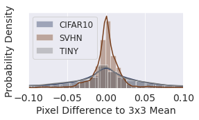
A

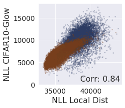
B

Conv Glow trained on:	Local Glow	Dense Glow	Conv Glow
CIFAR10	1.0	0.86	1.0
SVHN	0.96	0.90	0.97
TINY	1.0	0.86	1.0

C

Figure 1: Low-level features and model bias. A: Distributions over local pixel value differences have overlapping high-density regions for Tiny, SVHN, CIFAR10 . B: Likelihoods extracted from the local pixel-difference distributions correlate with CIFAR10-Glow likelihoods. C: Likelihood correlations for different types of Glow networks trained on CIFAR10 with regular convolutional Glow networks trained on CIFAR10, SVHN and Tiny. Correlations are almost the same for convolutional Glow networks and local Glow networks trained on $8\times 8$ patches. Correlations are smaller for fully-connected/dense Glow networks.

The following hypotheses synthesized from the findings of prior work motivate our methods to detect if an image is from a different object recognition dataset:

1. Distributions of low-level features form a domain prior valid for all natural images (see Fig. 1A).

2. These low-level features contribute the most to the overall likelihood assigned by a deep generative network to any image (see Fig. 1B and C).

3. How strongly which type of features contributes to the likelihood is influenced by the model bias (e.g., for convolutional networks, local features dominate) (see Fig. 1C).

For the first hypothesis, we start from defining low-level features. They are features that can be extracted in few computational steps (these will be local features for convolutional models like Glow). As an example, we use the difference of a pixel value to the mean of its $3\times 3$ neighbouring pixels. As natural images are smooth, the distributions over such per-pixel difference of SVHN, CIFAR10 and 80 Million Tiny Image (Tiny) depicted in Fig. 1A are all zero centered. Smoother images will produce smaller differences among neighbouring pixels, therefore the density of SVHN has the highest peak around zero. A significant overlapping high-density regions for SVHN, CIFAR10 and Tiny show that these low-level features are common to natural images, and thus not useful for anomaly detection.

Next, we examine the second hypothesis by showing that low-level per-image likelihoods highly correlate with Glow network likelihoods. On the pixel level, we compute the pixel difference and estimate its density using a histogram with $100$ equally distanced bins. Using the estimated density, we can get the conditional (on $3\times 3$ neighbours) per-pixel likelihoods of each image. Summing the per-pixel likelihoods over the entire image, we obtain pixel-level per-image pseudo-likelihood, which is not a correct likelihood of image, but a proxy measure of low-level feature contributions to the image-level likelihood. The low-level pseudo-likelihoods of SVHN and CIFAR10 images have Spearman correlations $>0.83$ with likelihoods of Glow networks trained on CIFAR10 (see Fig 1B), SVHN or Tiny. We also trained small modified Glow networks on $8\times 8$ patches cropped from the original image. These local Glow networks’ likelihoods correlate even more with the full Glow networks’ likelihoods ($>0.95$), further suggesting low-level local features dominate the total likelihood (see Fig 1C). To validate that the low-level features dominating the likelihoods are independent of the semantic content of the image, we mix two images in Fourier space by combining the amplitudes of one image’s Fourier transform with the phases of the other image’s Fourier transform, and then evaluate the likelihood of the resulting image using the same pretrained Glow model (see supp. material S3 for details). The mixed images are semantically much more coherent with the images that provide the phase information, yet their Glow likelihoods correlate more strongly with the Glow likelihoods of images sharing the same amplitudes ($>0.8$ vs. $<0.05$).

Lastly, we show that what features are extracted and how much each feature contributes to the likelihood depend on the type of model. When training a modified Glow network that uses fully connected instead of convolutional blocks (see supp. material S2.2) on Fashion-MNIST and MNIST, the image likelihoods among them do not correlate (Spearman correlation $-0.2$). The fully-connected Fashion-MNIST network achieves worse likelihoods ($4.8$ vs. $2.9$ bpd), but is much better at anomaly detection ($81\%$ AUROC for Fashion-MNIST vs. MNIST; $15\%$ AUROC for convolutional Glow).

Consistent with non-distribution-specific low-level features dominating the likelihoods, we find full Glow networks trained independently on CIFAR10, CIFAR100, SVHN or Tiny produce highly correlated image likelihoods (Spearman correlation $>0.96$ for all pairs of models, see Fig. 1 C). The same is true to a lesser degree for Fashion-MNIST and MNIST (Spearman correlation $0.85$).

Taken together, the evidence suggests convolutional generative networks have model biases that guide them to learn low-level feature distributions of natural images (domain prior) well, at the expense of anomaly detection performance. Based on this understanding, next we propose two methods to remove this influence of model bias and domain prior on likelihood-based anomaly detection.

3 Hierarchy of Distributions

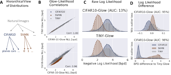
Figure 2: Overview of the hierarchy-of-distributions approach. A: Schematic hierarchical view of image distributions. To approximate the distribution of natural images, we use 80 Million Tiny images (Tiny). B,C,D: Results of Glow networks trained on CIFAR10, SVHN and Tiny. B: Likelihoods rank-correlate almost perfectly for the Glow networks trained on CIFAR10 and Tiny on all three datasets (top), while rank correlations remain very close to 1 for CIFAR10-Glow and SVHN-Glow (bottom), validating that the main likelihood contribution comes from the domain prior. C: Distribution plots show almost identical plots for CIFAR10 and Tiny-Glow and a low area under the receiver operating curve (AUC) for CIFAR10 vs. SVHN anomaly detection. D: In contrast, the log likelihood difference between CIFAR10-Glow and Tiny-Glow reaches substantially higher AUCs (top), further increased by using our outlier loss (bottom) (see Section 3.1).

The models trained on Tiny have the highest average likelihood across all evaluated datasets. This inspired us to use a hierarchy of distributions: CIFAR10 and SVHN are subdistributions of natural images, CIFAR10-planes are a subdistribution of CIFAR10, etc. (see Fig. 2).

We use this hierarchy of distributions to derive a log-likelihood-ratio-based anomaly detection method:

1. Train a generative network on a general image distribution like 80 Million Tiny Images

2. Train another generative network on images drawn from the in-distribution, e.g., CIFAR10

3. Use their likelihood ratio for anomaly detection

Formally, given the general-distribution-network likelihood $p_{g}$ and the specific-in-distribution-network likelihood $p_{in}$, our anomaly detection score (low scores indicate outliers) is:

$$\log\left(\frac{p_{\mathrm{in}}(x)}{p_{\mathrm{g}}(x)}\right)=\log\left(p_{\mathrm{in}}(x))-\log(p_{\mathrm{g}}(x)\right).$$ (1)

3.1 Outlier Loss

We also derive a novel outlier loss on samples $x_{\mathrm{g}}$ from the more general distribution based on the two networks likelihoods. Concretely, we use the log-likelihood ratio after temperature scaling by $T$ as the logit for binary classification:

$$L_{\mathrm{o}}=-\lambda\cdot\log\left(\sigma\left(\frac{\log(p_{\mathrm{g}}(x_{\mathrm{g}}))-\log(p_{\mathrm{in}}(x_{\mathrm{g}}))}{T}\right)\right)=-\lambda\cdot\log\left(\frac{\sqrt[T]{p_{\mathrm{g}}(x_{\mathrm{g}})}}{\sqrt[T]{p_{\mathrm{in}}(x_{\mathrm{g}})}+\sqrt[T]{p_{\mathrm{g}}(x_{\mathrm{g}})}}\right),$$ (2)

where $\sigma$ is the sigmoid function and $\lambda$ is a weighting factor.

3.2 Extension to the Supervised Setting

In all previous parts, our method is presented in an unsupervised setting, where the labels of the inliers are unavailable. We extend our method to the supervised setting with two main changes in our training. First, the Glow model $p_{\mathrm{in}}(x)$ uses a mixture of Gaussians for the latent $z$, i.e., each class corresponding to one mode. Second, the outlier loss is extended for each mode of $p_{\mathrm{in}}(x)$ by treating samples from the other classes as the negative samples, i.e., the same as $\{x_{\mathrm{g}}\}$ in Eq. 2.

4 Hierarchy of Features

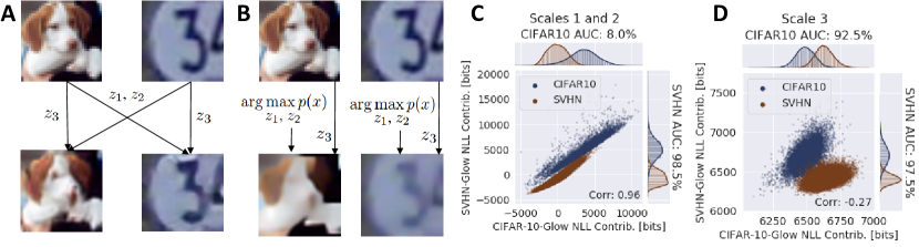
Figure 3: Overview of the hierarchy of features motivation. A,B: Showcasing features at different scales in the Glow-network. Top images are examples from CIFAR10 and SVHN. A: Bottom two images are obtained by mixing features in the Glow-network trained on CIFAR10 as follows. We compute the three scale outputs of the Glow-network $z_{1}$, $z_{2}$ and $z_{3}$, mix them between both images and invert again. For the bottom-left image, we take the earlier-scale features $z_{1}$ and $z_{2}$ from the SVHN image and the final-scale features $z_{3}$ from the CIFAR10 image and vice versa for the bottom-right image. Note the image class is completely determined by $z_{3}$. B: Images are optimized to maximize the CIFAR10-Glow-network likelihood $p(x)$ while keeping $z_{3}$ constant as follows. We keep $z_{3}$ from original Glow output fixed, and use the inverse pass of the network to optimize $z_{1}$ and $z_{2}$ via gradient ascent to maximize $\log(p(x))$. Only the global shape remains visible in the optimized images, while low-level structures have been blurred away. Such observation indicates that smoother local low-level features induce higher likelihood response of the model, once again confirming the strong influence of domain prior on the model likelhood. C,D: We use two Glow models trained on CIFAR10 and SVHN, respectively. The log likelihood they obtain on CIFAR10 and SVHN is split into log likelihood contributions of $z_{1}$, $z_{2}$ and $z_{3}$. The two plots show that (i) the summed contributions for $z_{1}$ and $z_{2}$ have very high rank correlation between both models (C); while the rank correlation drops for $z_{3}$ (D) and (ii) the range of the contributions is much larger for $z_{1}$ and $z_{2}$, showing that $z_{1}$ and $z_{2}$ dominate the total log likelihood.

The image likelihood correlations between models trained on different datasets reduce substantially when evaluating the likelihood contributions of the final scale of the Glow network (see Fig. 3). Here, the adopted Glow network has three scales. At the first two scales, i.e., $i=1$ and $2$, the layer output is split into two parts $h_{i}$ and $z_{i}$, where $h_{i}$ is passed onto the next scale and $z_{i}$ is output as one part of the latent code $z$. The output at the last scale is $z_{3}$, which together with $z_{1}$ and $z_{2}$ makes up the complete latent code $z$. In terms of $y_{1}=(h_{1},z_{1})$, $y_{2}=(h_{2},z_{2})$, $y_{3}=z_{3}$ and $h_{0}=x$, the logarithm of the learned density $p(x)$ can be decomposed into per-scale likelihood contributions $c_{i}(x)$ as

$$\log p(x)=\sum_{i}c_{i}(x)=\sum_{i}\log p_{\mathrm{z}}(z_{i})+\log\left|\mathrm{det}\left(\frac{\partial y_{i}}{\partial h_{i-1}}\right)\right|.$$ (3)

The log-likelihood contributions $c_{3}(x)$ of the final third scale of Glow networks correlate substantially less than the full likelihoods for Glow networks trained on the different datasets ($0.26$ mean correlation vs. $0.99$ mean correlation). This is consistent with the observation that last-scale dimensions encode more global object-specific features (see Fig. 3 and [4]). Therefore, we use $c_{3}(x)$ as our anomaly detection score (low scores indicate outliers).

Note that, here we do not condition $z_{1}$ on $z_{2}$ or $z_{2}$ on $z_{3}$, whereas other implementations often make $z_{1}$ dependent of $z_{2}$ such as $z_{1}\sim N(f(z_{2}),g(z_{2})^{2})$ with $f,g$ being small neural networks. Such dependency is removable by transforming to $z_{1}^{\prime}=\frac{(z_{1}-f(z_{2}))}{g(z_{2}))}$, with $z_{1}^{\prime}$ now independent of $z_{2}$ as $z_{1}^{\prime}\sim N(0,1)$, and this type of transformation can already be learned by an affine coupling layer applied to $z_{1}$ and $z_{2}$, hence the explicit conditioning of other implementations does not fundamentally change network expressiveness. We do not use it here and do not observe bits/dim differences between our implementation and those that use it (see supp. material S7.1 for details).

5 Experiments

For the main experiments, we use SVHN [24], CIFAR10 [14], CIFAR100 [15] as inlier datasets and use the same and LSUN [38] as outlier datasets. Results for further outlier datasets can be found in the supp. material S7.4. 80 Million Tiny Images [36] serve as our general distribution dataset in the log likelihood-ratio based anomaly detection experiments and is also used in the outlier loss as given in Eq. 2 when training two generative models, i.e., Glow and PixelCNN++ (PCNN) (see supp. material S4 for their training details). In-distribution Glow and PixelCNN++ models are finetuned from the models pre-trained on Tiny for more rapid training, see supp. material S7.2 for details and ablation studies. Our reported results are averaged over 3 random seeds.

5.1 Anomaly Detection based on Log-Likelihood Ratio

Table 1: Anomaly detection performance (AUCs in $\%$) of using the log-likelihood ratio of the in-distribution and general distribution model. For the general distribution models, we have three options, i.e., the general-purpose image compressor PNG [32] plus Tiny-Glow and Tiny-PCNN respectively trained on Tiny Images. Here, the Glow and PCNN trained on Tiny Images are also used as the starting point to train the in-distribution models. In the supp. material, we compare the results with training the two in-distribution models from scratch.

		Glow (in-dist.) diff to:				PCNN (in-dist.) diff to:
In-dist.	OOD	None	PNG	Tiny-Glow	Tiny-PCNN	None	PNG	Tiny-Glow	Tiny-PCNN
SVHN	CIFAR10	98.3	74.4	100.0	100.0	97.9	76.8	100.0	100.0
	CIFAR100	97.9	79.5	100.0	100.0	97.4	81.3	100.0	100.0
	LSUN	99.6	96.8	100.0	100.0	99.4	98.1	100.0	100.0
CIFAR10	SVHN	8.8	75.4	93.9	16.6	12.6	82.3	94.8	94.4
	CIFAR100	51.7	57.3	66.8	53.4	51.7	57.1	57.5	63.5
	LSUN	69.3	83.6	89.2	16.8	74.8	87.6	93.6	92.9
CIFAR100	SVHN	10.3	68.4	87.4	18.3	13.7	76.4	91.3	90.0
	CIFAR10	49.2	44.1	52.8	54.2	49.1	44.2	48.3	54.5
	LSUN	66.3	77.5	81.0	19.1	71.7	82.7	90.0	87.6
	Mean	61.3	73.0	85.7	53.2	63.2	76.3	86.2	87.0

In Tab. 1, we compare the raw log-likelihood based anomaly detection (i.e., diff to: None) with the log-likelihood ratio based ones (i.e., diff to: PNG, Tiny-Glow, Tiny-PCNN). The raw log-likelihood based scheme underperforms the log-likelihood ratio based ones that use Tiny-Glow and Tiny-PCNN. However, when using PNG to remove the domain prior as proposed in [32], it sometimes performs worse than the raw log-likelihood based scheme, e.g., SVHN as the in-distribution vs. the other three OODs. This relates to the remaining model bias, as Glow trained on the in-distribution encodes the domain prior differently to PNG. Also note that using PCNN as the general-distribution model for Glow does not work well for CIFAR10/100. This is because Tiny-PCNN has very large bpd gains over Glow for the CIFAR-datasets and less large gains for SVHN. On average across datasets, it works best to use matching general and in-distribution models (Glow for Glow, PCNN for PCNN), validating our idea of a model bias. Also note that our SVHN vs. CIFAR10 results already outperform the likelihood-ratio-based results of Ren et al. [27] slightly (93.9% vs. 93.1% AUROC), and we observe further improvements with outlier loss in Section 5.3. Ren et al. [27] used a noised version of the in-distribution as the general distribution and only tested it on SVHN vs. CIFAR10. Comparing to Tiny, it is less representative as a domain prior, and thus its performance on more complicated datasets requires further assessment.

Medical Dataset

To further validate our log-likelihood ratio approach on a different domain, we setup an experiment on the medical BRATS Magnetic Resonance Imaging (MRI) dataset. We use one MRI modality as in-distribution and the other three as OOD. The raw likelihood, the log-likelihood ratio to Tiny-Glow and to BRATS-Glow (trained on all modalities) yield AUROC $53.3\%$, $68.3\%$ and $78.3\%$, respectively. So, Tiny also serves as a general distribution for the very different medical images, and a distribution from the more specific domain further improves the performance.

The log-likelihood ratio approach can likely be applied to more than images. In the above, we have already shown the application to typical image datasets and, without adaptation, to medical MRI images. In the text/NLP domain, it may be used with Wikitext-2 as the general dataset, since Wikitext-2 already worked well as an outlier dataset in [8]. In the audio domain, the domain prior may come from strong dependencies of the signal values on short timescales, similar to the smoothness of natural images. If a suitable general dataset needs to be created, it does not require labels and may even profit from noisy/unclean data. Therefore there is no principal obstacle preventing collection of such data, including concatenating existing datasets.

5.2 Anomaly Detection based on Last-scale Log-likelihood Contribution

As an alternative to remove the domain prior by using, e.g., Tiny-Glow, our hierarchy-of-features view suggests to use the log-likelihood contributed by the high-level features attained at the last scale of the Glow model. It is orthogonal to the log-likelihood ratio based scheme, and can be used when the general distribution is unavailable. As shown in Tab. 3, using the raw log-likelihood on the last scale ($4\times 4$), consistently outperforms the conventional log-likelihood comparison on the full scale, but performs slightly worse than using the log-likelihood ratio in the full scale. Note that we don’t expect the log-likelihood ratio on the last scale to be the top performer, as the domain prior is mainly reflected by the earlier two scales, see Fig. 3.

Table 2: Raw log-likelihoods vs. log-likelihood ratios on different scales, where CIFAR10 is the in-distribution.

Out-dist	Scale	Raw	Diff
SVHN	Full	8.8	93.9
	16x16	7.0	84.6
	8x8	13.5	48.9
	4x4	92.9	83.6
CIFAR100	Full	51.7	66.8
	16x16	50.7	55.7
	8x8	53.5	56.3
	4x4	60.0	66.1
LSUN	Full	69.3	89.2
	16x16	70.3	63.6
	8x8	56.5	74.0
	4x4	82.8	75.1

Table 3: Different outlier losses, where CIFAR10 is the in-distribution.

Out-dist	Loss	Raw	4x4	Diff
SVHN	None	8.8	92.9	93.9
	Margin	84.2	84.2	96.5
	Ours	95.5	96.4	98.6
CIFAR100	None	51.7	60.0	66.8
	Margin	72.3	71.7	71.1
	Ours	84.9	85.4	84.5
LSUN	None	69.3	82.8	89.2
	Margin	82.0	82.0	75.7
	Ours	94.9	95.1	94.1

5.3 Outlier Losses

When training the in-distribution model, we can use the images from Tiny as the outliers to improve the training. Tab. 3 shows that our outlier loss as formulated in Eq. 2 consistently outperforms the margin loss [8] when combining with three different types of log-likelihood based schemes, i.e., raw log-likelihood, raw log-likelihood at the last scale $4\times 4$ and log-likelihood ratio. We note that as the margin loss leads to substantially less stable training than our loss, see the supp. material S7.5.

We also experiment on adding the outlier loss to the training loss of Tiny-Glow, i.e., using the in-distribution samples as outliers. This further improves the anomaly detection performance, see Diff† of Tab. 4, while Diff only uses the outlier loss for training the in-distribution Glow-network.

5.4 Unsupervised vs. Supervised Setting

From the unsupervised to the supervised setting, Tab. 4 further reports the numbers achieved by using the class-conditional in-distribution Glow-network and treating inputs from other classes as outliers. We observe further improved anomaly detection performance.

Table 4: Anomaly detection performance summary (AUC in $\%$). The new term Diff† means to use in-distribution samples as the outliers to train Tiny-Glow, see Sec. 5.4. OE, proposed by Hendrycks et al. [8], stands for margin-based outlier loss for PixelCNN++, MSP-OE from the same work stands for entropy of classifier predictions with entropy outlier loss.

	Setting	Unsupervised				Supervised
In-dist	Out-dist	4x4	Diff	Diff†	OE	4x4	Diff	Diff†	MSP-OE
CIFAR10	SVHN	96.4	98.6	99.0	75.8	96.1	98.6	99.1	98.4
	CIFAR100	85.4	84.5	86.8	68.5	88.3	87.4	88.5	93.3
	LSUN	95.1	94.1	95.8	90.9	95.3	94.1	96.2	97.6
	Mean	92.3	92.4	93.8	78.4	93.3	93.4	94.6	96.4
CIFAR100	SVHN	84.5	82.2	85.4	-	89.6	88.6	89.4	86.9
	CIFAR10	61.9	59.8	62.5	-	67.0	64.9	65.3	75.7
	LSUN	84.6	82.4	85.4	-	85.7	84.3	86.3	83.4
	Mean	77.0	74.8	77.8	-	80.8	79.3	80.3	82.0
	Mean	84.7	83.6	85.8	-	87.0	86.3	87.5	89.2

Overall, our approach only slightly underperforms the approach MSP-OE [8] with inlier class labels (Supervised), while being substantially better without inlier class labels (Unsupervised), see Tab. 4. In contrast to observations by Hendrycks et al. [8] for their unsupervised setup, we do not experience a severe degradation of the anomaly detection performance from the lack of class labels.

6 Related Work

We present an overview over anomaly detection approaches with a focus on recent work closely related to the ideas of a hierarchy of distributions and a hierarchy of features.

Classifier-based Methods Multi-class classifiers trained to discriminate in-distribution classes have been used for anomaly detection. Hendrycks and Gimpel [7] used maximum softmax response as the score of normality. Different data augmentation schemes [19, 17, 8, 9] further enforced its performance. Lee et al. [18] alternatively modeled the class-conditional features attained by the hidden layers of the classifier as multivariate Gaussians, and then used the Mahalanobis distance of Gaussians for anomaly detection. Another recent work [6] used the gradient norm of the log-sum-exp of the class logits over the input for anomaly detection. In the context of self-supervised learning, class becomes the type of transformations [2, 5]. Self-supervised contrastive training improved the anomaly detection performance of multi-class classifiers [37].

Instead of exploiting multi-class classifiers, a different approach is to train a one-class classifier to directly discriminate inliers and outliers. One-class support vector machines are trained to return positive values only in a small region containing the inliers and negative values elsewhere [31]. This approach has also been used in forming the latent space of deep autoencoders [28, 29, 30]. Ruff et al. [30] also used samples from a general distribution as outliers. Steinwart et al. [34] drawn outliers from uniform distribution. In the supp. material S9, we also report results using a in-distribution-vs-general-distribution classifier.

Reconstruction-based Methods Another line of work is to learn the features and generation of inliers by reconstructing the training samples either in their input space or latent space, e.g., [26, 25, 1, 11]. At test time, an outlier is then detected if reconstruction is poor. However, owing to large capacity of deep neural networks, reconstruction loss alone may not be a reliable metric for anomaly detection. Huang et al. [10] proposed to additionally use the joint likelihood of latent variables, which is obtained by using a neural rendering model to invert multi-class CNN-based classifier.

Input Likelihood-based Methods Generative modeling through maximum likelihood estimation tries to enforce high likelihoods on inliers. Under the normalization constraint, the likelihoods of outliers are expected to be low (ideally zero). However, their anomaly detection performance is often unsatisfactory [33, 22, 8]. Outliers may attain even higher likelihoods than inliers. Recent work [23] related the poor performance to sampling in a high-dimensional space, namely, inliers being mapped to the typical set of the latent code rather than the high likelihood area. They proposed to address this issue by batch-wise anomaly detection, whose application is more limited than instance-wise anomaly detection. A different approach [3] combined input likelihoods with inlier classifiers. Che et al. [3] trained a class-conditional generative model with an auxiliary adversarial loss to disentangle the class information from the rest latent representation. The achieved performance is better than ours in the supervised setting, while our methods mainly target and work in the unsupervised setting. It can be interesting to exploit their way of incorporating the label information into our model training.

Our work is also input likelihood-based. Our analysis in Section 2 showed that convolutional networks trained on one natural image dataset will learn low-level feature distribution that is common to the whole domain, and such domain prior dominates the likelihood. The concurrent work [13] found results consistent with ours. We further exploited hierarchies of distributions or hierarchies of features as explained in Section 3 and 4 to improve the anomaly detection performance.

Hierarchy of Distributions: Our hierarchy-of-distributions likelihood-ratio method relates to prior [27] and concurrent [32] methods as follows. Ren et al. [27] used a noised version of the in-distribution as the general distribution. Their method always requires training of two models for each in-distribution, our method has the option of only require one training of a general distribution model which we can reuse for any new in-distribution as long as it is as a subdistribution of the general distribution. In our method, the challenge is to find a suitable general distribution, while in their method the challenge is to find a suitable noise model. In the only rgb-image-setting they evaluated in [27], we show improved results over theirs, see Section 5.1. Serrà et al. [32] used a generic lossless compressor such as PNG as their general distribution model and unfortunately only reported results on the training set of the in-distribution, making their results incomparable with any other works. We show improved performance over a reimplementation (see code repository) in Section 5.1. Note that both [27] and [32] did not evaluate the cases where raw likelihoods work well, even though using the likelihood ratio may decrease performance in that case as seen in Section 5.1.

Outlier Loss: Hendrycks et al. [8] used a margin loss on images from a known outlier distribution (Tiny without CIFAR-images). We develop an outlier loss to improve the performance of likelihood models. It can be viewed as a combination of their idea of an outlier loss with our view of a hierarchy of distributions, and achieved an improved performance in the unsupervised setting in Section 5.3.

Hierarchy of Features: Regarding hierarchy of features, the closest related work investigated deep variational autoencoders that use a hierarchy of stochastic variables and found that later stochastic variables perform better at anomaly detection [21]. Furthermore, Krusinga et al. [16] developed a method to approximate probability densities from generative adversarial networks. The log densities are the sum of a change-of-volume determinant and a latent prior probability density. The latent log densities better reflected semantic similarity to the in-distribution than the full log density, however, no comparable anomaly detection results were reported. Nalisnick et al. [22] also found the same for latent vs. full log densities of Glow networks, but also did not report anomaly detection results and did not look at individual scales of Glow networks.

7 Discussion and Conclusion

In this work, we proposed two log-likelihood based metrics for anomaly detection, outperforming state of the art methods in the unsupervised setting and only slightly underperforming classifier-based methods in the supervised setting. For good anomaly detection performance from raw likelihoods, an additional loss (such as our outlier loss) that forces the model to assign low likelihoods for images with OOD-high-level features, e.g. wrong objects, is particularly beneficial according to empirical results. Our analysis points to a potential reason, namely that without an outlier loss, the likelihoods are almost fully determined by low-level features such as smoothness or the dominant color in an image. As such low level features are common to natural image datasets, they form a strong domain prior, presenting a difficult task to detect high-level differences between inliers and outliers, e.g., object classes.

An interesting future direction is how to best combine the hierarchy-of-distributions and hierarchy-of-features views into a single approach. Preliminary experiments freezing the first two scales of the Tiny-Glow model and only finetuning the last scale on the in-distribution have shown promise, awaiting further evaluation.

In summary, our approach shows strong anomaly detection performance particularly in the more challenging unsupervised setting and also allows a better understanding of generative-model-based anomaly detection by leveraging hierarchical views of distributions and features.

Broader Impact

A better understanding of deep generative networks with regards to anomaly detection can help the machine learning research community in multiple ways. It allows to estimate which tasks deep generative networks may be suitable or unsuitable for when trained via maximum likelihood. With regards to that, our work helps more precisely understand the outcomes of maximum likelihood training. This more precise understanding can also help guide the design of training regimes that combine maximum likelihood training with other objectives depending on the task, if the task is unlikely to be solved by maximum likelihood training alone.

Anomaly detection in general itself has positive uses. For example, detecting anomalies in medical data can detect existing and developing medical problems earlier. Safety of machine learning systems in healthcare, autonomous driving, etc., can be improved by detecting if they are processing data that is unlike their training distribution.

Negative uses and consequences of anomaly detection can be that it allows tighter control of people by those with access to large computer and data, as they can more easily find unusual patterns deviating from the norm. For example, it may also allow health insurance companies to detect unusual behavioral patterns and associate them with higher insurance costs. Similarly repressive governments may detect unusual behavioral patterns to target tighter surveillance.

These developments may be steered in a better direction by a better public understanding and regulation for what purpose anomaly-detection machine-learning systems are developed and used.

Supplementary outline

This document completes the presentation of the main paper with the following:

1. Details about Glow and PixelCNN++ architectures, and the likelihood decomposition equation Eq. (3) of Sec. 4 in the main paper;

2. Details about the modified (local/fully connected) Glow architectures for the analysis in Sec. 2 of the main paper;

3. Fourier-based analysis of influence of amplitude and phase on likelihoods;

4. Details about training and evaluation of Glow and PixelCNN++, including hyperparameter choices and computing infrastructure;

5. Details on the used datasets and dataset splits;

6. Reasons why the results of Serrà et al. [32] are not comparable as is, and details of our reimplementation;

7. Further quantitative results, including maximum-likelihood performance (S7.1), finetuning vs. from-scratch training (S7.2), variance over seeds (S7.3), further outlier datasets (S7.4) and different outlier losses (S7.5);

8. Qualitative analysis of the different anomaly detection metrics;

9. Generative vs. discriminative approach for anomaly detection.

Please also note the attached supplementary codes.

Appendix S1 Glow and PixelCNN++ architectures

S1.1 Glow Network architecture

Our implementation of the Glow network [12] is based on a publicly available Glow implementation with one modification explained in S1.3. The multi-scale Glow network consists of three sequential scales processing representations of size $12\times 16\times 16$, $24\times 8\times 8$ and $48\times 4\times 4$ (channel $\times$ width $\times$ height). Each scale consists of a repeating sequence of activation normalization, invertible $1\times 1$ convolution and affine coupling blocks, see the original paper [12] for details. Our Glow network, consistent with aforementioned public implementation, uses $32$ actnorm-$1$ conv-affine sequences per scale.

S1.2 PixelCNN++ architecture

We use a publicly available PixelCNN++ implementation with only a single change. We reduce the number of filters used across the model from $160$ to $120$ for fast single-GPU training.

S1.3 Independent $z_{1}$, $z_{2}$, $z_{3}$

For a multi-scale model like Glow, the overall likelihood consists of the contributions from different scales, see Eq. (3) in the main paper. In contrast to other implementations, we do not condition $z_{1}$ on $z_{2}$ or $z_{2}$ on $z_{3}$ in our Glow model as described in Sec. S1.1. Recall that Glow splits the complete latent code into per-scales latent codes $z_{1}$, $z_{2}$, $z_{3}$. Here, $z_{1}$ is the half of the output of the first scale that is not processed further. Many implementations make $z_{1}$ dependent of $z_{2}$ (and same for $z_{2}$ and $z_{3}$) as $z_{1}\sim N(f(z_{2}),g(z_{2})^{2})$ with $f,g$ being small neural networks. For ease of implementation, we do not do that, instead we directly evaluate $z_{1}$ under a standard-normal gaussian, so $z_{1}\sim N(0,1)$.

Note that this does not fundamentally alter network expressiveness. An affine coupling layer can already implement the same computation achieved by $z_{1}\sim N(f(z_{2}),g(z_{2})^{2})$. Imagine $z$ is split for the affine coupling layer into $z_{1}$ and $z_{2}$, with a coefficient network on $z_{2}$ used to compute the affine scale and translation coefficients $s,t$ to transform $z_{1}^{\prime}=z_{1}\odot s(z_{2})+t(z_{2})$. Then if $s(z_{2})=-f(z_{2})$ and $t(z_{2})=\frac{1}{g(z_{2})}$ and $z_{1}\sim N(f(z_{2}),g(z_{2})^{2})$, it follows that $z_{1}^{\prime}\sim N(0,1)$. In other words, computing the mean and standard deviation for $z_{1}$ from $z_{2}$ is the same as normalizing $z_{1}$ by subtracting the mean and dividing by the standard deviation computed from $z_{2}$, which a regular affine coupling block can already learn.

In practice, there could still be differences due to the additional parameters, different kind of blocks used to implement $f$ and $g$, and the difference of computing the (log)$std$ or its inverse. However, we observe no appreciable bits/dim differences between our implementation and those using the explicit conditioning step, see Section S7.1.

Appendix S2 Local and Fully Connected Architectures

S2.1 Local Patches

We designed our local patches experiment to train compact Glow-like models that can only process information from $8\times 8$ patches in the original datasets. Full-sized Glow networks process the full image using three scales as written in Section S1.1. Our local Glow network instead processes local $8\times 8$ patches using a single scale. The $32\times 32$ input image is first cropped into $16$ non-overlapping $8\times 8$ patches. These $8\times 8$ patches are then processed independently by a local Glow network corresponding to a single scale of the full Glow network. In other words, we treat the image as if it consists of independent $8\times 8$ patches. Evaluating the likelihoods of these patches, their sum is the likelihood of the image assigned by the local Glow model. Note that we aimed to create a network restricted to learn a general local domain prior and not one with the best maximum-likelihood performance.

S2.2 Fully Connected

We designed our fully-connected experiment to train fully-connected Glow networks that have a different model bias to regular convolutional Glow networks. We kept the three-scale architecture of Glow including the invertible subsampling steps at the beginning of each scale. Within each scale, the fully-connected Glow first flattens the representation, e.g. from a $12\times 16\times 16$ tensor per rgb-image to a $3072$-sized vector in the scale $1$. This vector is then processed by the usual sequence of actnorm-$1\times 1$-affine. We next detail the processing at the scale $1$, whereas the other scales follow the same design pattern. Activation normalization now processes $3072$ dimensions, so has substantially more parameters. The $1\times 1$ is now an invertible linear projection keeping the dimensionality, so a projection from $3072$ dimensions to $3072$ dimensions. To ensure training stability, we did not train the $1\times 1$-projections, but kept their parameters in the randomly initialized starting state. The fully-connected affine coupling block uses a sequence of linear layer ($1536\times 512$) - ReLU - linear layer ($512\times 512$) - ReLU - linear layer ($512\times 3072$) modules to compute the $1536$ translation and $1536$ scale coefficients. To allow fast single-GPU training, we reduced the number of actnorm-$1\times 1$-affine sequences from $32$ to $8$ per scale. Similar to Section S2.1, the fully-connected network was designed to highlight the influence different model biases and not to reach the best maximum-likelihood performance.

Appendix S3 Fourier-based Amplitude/Phase Analysis

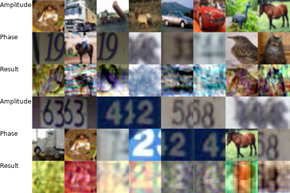
Figure S1: Image Mixup in frequency domain via Fourier transform. Fourier amplitudes taken from one image, phases from another and then inverted back to input space (Result). Note semantic content is more similar to phase image than to amplitude image.

To validate that low-level features dominate the likelihoods independent of the semantic content of the image, we create mixed images in Fourier space. Concretely, we:

1. Compute the amplitudes and phases of a batch Fourier transformed images;

2. Mix up images in their frequency domain by using one image’ amplitudes and phases of the other image

3. Apply the inverse Fourier transformation to invert these mixed images to the input domain

We show examples in Figure S1. Note that the mixed images are semantically much more similar to the image the phases were extracted from. We then compare the CIFAR10-Glow likelihoods on the original images and the mixed images for SVHN and CIFAR10 images. The likelihoods of the mixed images correlate much more with the amplitude-image likelihoods (Spearman correlation $>0.8$) than with the phase-image likelihoods (Spearman correlation $<0.05$).

Appendix S4 Training and Evaluation

S4.1 Glow Training

We stayed close to the training setting of a publicly available Glow repository. Namely, we use Adamax as the optimizer (learning rate $5\cdot 10^{-4}$, weight decay $5\cdot 10^{-5}$) and $250$ training epochs. The training setting also includes data augmentation (translations and horizontal flipping for CIFAR10/100, only translations for SVHN, Fashion-MNIST and MNIST). These settings are the same for all experiments (from-scratch training, finetuning, with and without outlier loss, unsupervised/supervised). On 80 Million Tiny Images, we use substantially less training epochs, so that the number of batch updates is identical between Tiny and the other experiments. All datasets were preprocessed to be in the range $[-0.5,0.5-\frac{1}{256}]$ as is standard practice for Glow-network training, see also supplementary code.

S4.2 PixelCNN++ Training

We stayed close to the training setting of the public PixelCNN++ repository. Namely, we use Adam as the optimizer (learning rate $2\cdot 10^{-4}$, no weight decay, negligible learning rate decay $5\cdot 10^{-6}$ every epoch). We substantially reduced the number of epochs from $5000$ to $120$ to save GPU resources, and since our aim here was to show general applicability of our methods to another type of model and not to reach maximum possible performance. Consistent with the public implementation, no data augmentation is performed.

S4.3 Numerical stabilization of the training

When training networks with outlier loss, negative infinities can appear for numerical reasons. This is actually expected as true outliers should ideally have likelihood zero and therefore log likelihood equal to negative infinity. These do not contribute to the loss in theory, but cause numerical issues. To ensure numerical stability during training, we remove examples that get assigned negative infinite likelihoods from the current minibatch. In case this would remove more than $75\%$ of the minibatch, we skip the entire minibatch. These methods are only meant to ensure numerical stability, no specific training stability methods like gradient norm clipping are used.

S4.4 Outlier Loss Hyperparameters

As described in the main manuscript, our outlier loss is:

$$L_{\mathrm{o}}=-\lambda\cdot\log\left(\sigma\left(\frac{\log(p_{\mathrm{g}}(x_{\mathrm{g}}))-\log(p_{\mathrm{in}}(x_{\mathrm{g}}))}{T}\right)\right)=-\lambda\cdot\log\left(\frac{\sqrt[T]{p_{\mathrm{g}}(x_{\mathrm{g}})}}{\sqrt[T]{p_{\mathrm{in}}(x_{\mathrm{g}})}+\sqrt[T]{p_{\mathrm{g}}(x_{\mathrm{g}})}}\right),$$ (S1)

where $\sigma$ is the sigmoid function, $T$ a temperature and $\lambda$ is a weighting factor. Based on a brief manual search on CIFAR10, we use $T=1000$ $\lambda=6000$ as they had the highest train set anomaly detection performance while retaining stable training. PixelCNN++ training works well with the same exact values, validating the choice.

S4.5 Evaluation Details

We use the likelihoods computed on noise-free inputs for anomaly detection with Glow networks. In practice, this means not adding dequantization noise and instead adding a constant, namely half of the dequantization interval. We found this to yield slightly better anomaly detection performance in preliminary experiments. Noise-free inputs are only used during evaluation for the anomaly detection performance. Training is done adding the standard dequantization noise introduced as in [35]. The BPD numbers reported in Section S7.1 and Table S1 also are obtained using single samples with the standard dequantization noise.

We clip log likelihoods from below by a very small number. When computing the log likelihoods from networks trained with outlier loss, negative infinities are to be expected, see Section S4.3. To include these inputs in the AUC computation, we set non-finite log-likelihoods to a very small constant ($-3000000$) before computing any log-likelihood difference.

S4.6 Computing Infrastructure

All experiments were computed on single GPUs. Runtimes vary between $2$ to $8$ days on Nvidia Geforce RTX 2080 depending on the experiment setting (outlier loss or not, supervised/unsupervised).

Appendix S5 Datasets

S5.1 Dataset Splits

We use the pre-defined train/test folds on CIFAR10, CIFAR100, SVHN, Fashion-MNIST and MNIST and only train on the training fold. All results are reported on the test folds. For CelebA, we only use the first $60000$ images for faster computations. We use a $1$ million random subset of 80 Million Tiny Images in all of our experiments. For the Fashion-MNIST/MNIST experiments, we create a greyscaled Tiny dataset from the rgb data as $x=r\cdot 0.2989+g\cdot 0.5870+b\cdot 0.1140$.

S5.2 MRI Dataset

For the MRI BRATS dataset, we also use the official train/test split. The dataset was introduced to verify the log likelihood difference on a data from a slightly different domain (medical imaging). Since our outliers defined as different modalities are not defined by the object type, we did not expect last-scale likelihood contributions $c_{3}(x)$ to perform as good as on the object recognition datasets. However, they still outperform raw likelihoods, by 59.2% to 53.3%.

Appendix S6 Replication of [32]

The anomaly detection results from [32] were obtained using the training folds of the in-distribution datasets, preventing a fair comparison to our results. In written communication with Serrà et al. [32], they explained to us that the AUROC-results reported in their paper compare in-distribution training-fold examples with out-of-distribution test-fold examples. This makes a fair comparison to our results and other works impossible. In contrast and in line with standard practice, our results were obtained using the test folds of the in-distribution datasets. Unfortunately, Serrà et al. [32] are unable to provide their training code and models at the current time, so we cannot recompute their anomaly detection performance for the test fold of the in-distribution datasets. We also confirmed that depending on the training setting, the anomaly-detection AUROC values can differ substantially between the training and test fold of the in-distribution dataset.

In any case, we provide supplementary code to reproduce the method of[32] to the best of our understanding. Using a publicly available pretrained Glow-model, we find anomaly detection performance results similar to the ones we report for PNG as a general-distribution model.

Appendix S7 Further Quantitative Results

S7.1 Maximum Likelihood Performance

The maximum-likelihood-performance of our finetuned Glow networks are similar to the performance reported for from-scratch training in the original Glow paper [12]. We show the bits-per-dimension values obtained using single dequantization samples in Table S1. Note that the Glow model trained on 80 Million Tiny Images already reaches bits per dimensions on CIFAR10 and CIFAR100 close to the Glow models trained on the actual dataset (CIFAR10/CIFAR100), in line with our view that the bits per dimension are dominated by the domain prior (results also do not substantially change when including or excluding CIFAR-images from Tiny).

Our Glow-model architecture was chosen from a reimplementation of Nalisnick et al. [22] (see Section S1.1), in order to facilitate comparison of our results to other anomaly detection works. In future work, evaluating anomaly detection performance of our method with newer types of normalizing flows could be interesting.

Table S1: Maximum likelihood performance in bits per dimension. Results obtained using single samples of uniform dequantization noise. Tiny is the Glow network trained on 80 Million Tiny Images. Retr refers to from-scratch training on the in-distribution dataset, Finet refers to finetuning aforementeioned Glow network trained on 80 Million Tiny Images. Note the original Glow paper [12] reached 3.35 bpd on CIFAR-10 with multi-GPU training. The Glow network and training setup we use is optimized for single-GPU training and not for maximum performance. The public implementation we originally based our implementation on (and uses the explicit conditioning step discussed in S1.3) reaches $3.39$ bpd on CIFAR10.

In-dist	Tiny	Retr	Finet
SVHN	2.34	2.07	2.06
CIFAR10	3.41	3.40	3.36
CIFAR100	3.43	3.43	3.39

S7.2 Finetuning

Training Glow networks on an in-distribution dataset by finetuning a Glow network trained on Tiny substantially speeds up the training progress over training from scratch. As can be seen in Figures S3 and S2, the Glow networks reach better results after less training epochs for both maximum-likelihood performance and anomaly-detection performance. The improvements are strongest for CIFAR100 and weakest for SVHN, in line with CIFAR100 being the most diverse dataset and most similar to 80 Million Tiny Images.

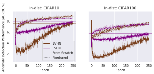
Figure S2: Training Curves Anomaly Detection From Scratch vs. Finetuned. Conventions as in Fig. S3. Glow networks are trained without any outlier loss. AUROC refers to AUROC computed from our log-likelihood ratio metric using another Glow-network trained on 80 Million Tiny Images. Note that the finetuned Glow networks outperform the final from-scratch trained Glow networks after less than $20\%$ of the training epochs. Note that due to different evaluation (not noise-free) and different subsets used for intermediate results, results in this figures vary from final results in result tables.

CIFAR10/100

SVHN

Figure S3: Training Curves CIFAR10/100 and SVHN From Scratch vs. Finetuned. Transparent, thin lines indicate single-seed runs, solid, think lines indicate means over these runs. Solid horizontal lines indicate final mean performance of from-scratch trained models. Note that (i) finetuned Glow networks are better in each epoch; (ii) for CIFAR10/100 the finetuned Glow networks outperform the final from-scratch trained Glow networks after less than $20\%$ of the training epochs and (iii) for SVHN, the finetuned Glow network outperforms the final from-scratch-trained Glow network after about 50% of the training epochs.

Figure S4: Training Curves Anomaly Detection Finetuned from Own model vs Finetuned from Tiny. Conventions as in Fig. S2. Finetuned from own model is the same as simply training twice as long on the in-distribution. At the end of training for CIFAR100, the model finetuned from Tiny still performs ~6% better on anomaly detection.

There are are still gains on log-likelihood ratio based anomaly detection for CIFAR100 when comparing finetuning a Glow a Glow network trained on Tiny to finetuning a Glow network already trained on CIFAR100 (or in other words, training the Glow Network from scratch on CIFAR100 for twice the number of epochs), see Figure S4. This is likely because the exact Tiny-model be used as the general distribution model later on, validating more similar models better cancel the model bias.

S7.3 Result Variance across Seeds

We present the original results including standard deviation in Table S2 and provide a graphical overview over our per-seed anomaly detection results in Figure S5. Results are relatively stable across seeds.

S7.4 Additional OOD Datasets

We report results on CelebA [20] and Tiny Imagenet as additional out-of-distribution (OOD) datasets in Table S3.

Table S2: Anomaly detection performance summary (AUC in $\%$). Values in parentheses are standard deviation across 3 seeds. The new term Diff† means to use in-distribution samples as the outliers to train Tiny-Glow, see Sec. 5.4 in main paper.

	Setting	Unsupervised			Supervised
In-dist	Out-dist	4x4	Diff	Diff†	4x4	Diff	Diff†
CIFAR10	SVHN	96.4 (1.4)	98.6 (0.1)	99.0 (0.1)	96.1 (1.7)	98.6 (0.1)	99.1 (0.1)
	CIFAR100	85.4 (0.7)	84.5 (0.6)	86.8 (0.5)	88.3 (0.7)	87.4 (0.5)	88.5 (0.3)
	LSUN	95.1 (1.2)	94.1 (1.5)	95.8 (0.8)	95.3 (1.1)	94.1 (1.7)	96.2 (0.9)
	Mean	92.3 (1.0)	92.4 (0.6)	93.8 (0.4)	93.3 (1.2)	93.4 (0.8)	94.6 (0.4)
CIFAR100	SVHN	84.5 (2.1)	82.2 (3.1)	85.4 (2.1)	89.6 (1.0)	88.6 (0.8)	89.4 (0.7)
	CIFAR10	61.9 (0.5)	59.8 (0.5)	62.5 (0.3)	67.0 (0.6)	64.9 (0.8)	65.3 (0.7)
	LSUN	84.6 (0.1)	82.4 (0.3)	85.4 (0.1)	85.7 (0.4)	84.3 (0.3)	86.3 (0.2)
	Mean	77.0 (0.7)	74.8 (1.1)	77.8 (0.6)	80.8 (0.7)	79.3 (0.6)	80.3 (0.5)
	Mean	84.7 (0.3)	83.6 (0.3)	85.8 (0.2)	87.0 (0.9)	86.3 (0.7)	87.5 (0.4)

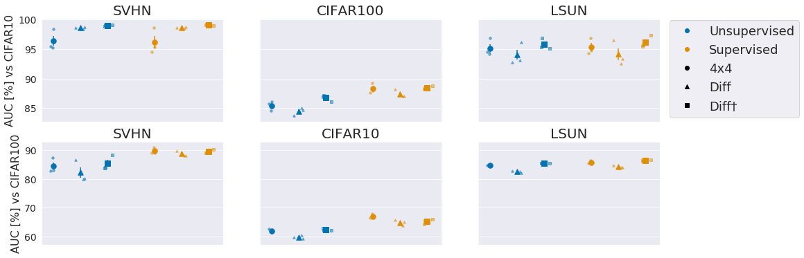
Figure S5: Graphical Overview over Anomaly Detection Results. Markers indicate mean result over three seeds, error bars indicate standard error of that mean. Type of marker indicates type of anomaly metric (defined as before and as in Table S2). Color indicates supervised or unsupervised setting. Rows are in-distribution dataset and columns are OOD datasets. Supervised setting outperforms unsupervised setting, especially on CIFAR10 vs. CIFAR100 and vice versa. Using a general-distribution model trained with outlier loss on the in-distribution (Diff†) always outperforms general-distribution model trained without outlier loss (Diff). Relative performance of final-scale method ($4\times 4$) compared with log-likelihood-difference methods (Diff and Diff†) varies between dataset pairs.

Table S3: Anomaly detection performance for additional OOD datasets CelebA and Tiny-Imagenet. Conventions as in Table main manuscript.

	Setting	Unsupervised			Supervised
In-dist	Out-dist	Raw [4x4]	Diff	Diff†	Raw [4x4]	Diff	Diff†
CIFAR10	CelebA	96.6 (1.2)	96.1 (1.2)	97.6 (0.5)	96.6 (1.9)	96.2 (2.1)	97.8 (1.0)
	Tiny-Imagenet	90.7 (0.9)	90.6 (0.7)	92.1 (0.4)	91.1 (0.8)	91.3 (0.9)	92.7 (0.4)
CIFAR100	CelebA	80.9 (1.3)	76.4 (2.4)	80.4 (1.1)	81.9 (5.4)	79.1 (7.2)	81.7 (4.7)
	Tiny-Imagenet	77.3 (0.5)	77.5 (0.5)	79.7 (0.3)	79.5 (0.4)	79.7 (0.5)	80.6 (0.5)

S7.5 Margin Loss vs. Outlier Loss

In our experiments, the margin-based loss introduced in [8] is less stable than our outlier loss for longer training runs, see Figure S6. Note that our results for the margin-based loss already substantially outperform the results reported for PixelCNN with a margin-based loss in [8].

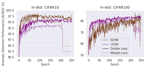
Figure S6: Training Curves Anomaly Detection Margin Loss vs Outlier Loss. AUROC refers to AUROC computed from our log-likelihood-difference metric using another Glow-network trained on 80 Million Tiny Images. Note Glow networks trained with margin loss experience substantial drops in anomaly detection performance in later stages of the training.

Appendix S8 Qualitative Analyses

Our different metrics (raw likelihoods, log-likelihood ratios and last-scale likelihood contributions) result in qualitatively different highest-scoring images on 80 Million Tiny Images (see Fig. S7 and S8). We take a random 120000-images subset of 80 Million Tiny Images and use our Glow network trained on CIFAR10 either with or without outlier loss to compute the metrics. Looking at the top 12 images per metric shows that using the log-likelihood ratio results in more reasonable images (closer to the inliers) than the raw likelihood, albeit mostly still simple images (see Fig. S7) and that using the Glow network trained with outlier loss results in more fitting images for all metrics (see Fig. S8).

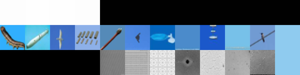
Figure S7: Most likely images from 80 Million Tiny Images for CIFAR10-Glow. 12 highest-scoring images selected according to different metrics. First row: raw likelihood, second row: log-likelihood ratio to Tiny-Glow, third row: raw last-scale $z_{3}$ likelihood contribution. Note that constant images attain the highest raw likelihood, showing the effect of the natural-images domain prior on the raw likelihoods. The highest-scoring log-likelihood-ratio images show a bias towards blue images and some contain actual CIFAR10 objects, namely birds and planes. Overall, the difference selects some correct images, but is still sensitive to surface features such as the global color. The last-scale results are harder to interpret, the more diverse images suggest it is slightly less affected by the domain prior of smoothness.

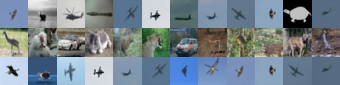
Figure S8: Most likely images from 80 Million Tiny Images for CIFAR10-Glow with the outlier loss. Conventions as in Figure S8. Now any of the three metrics lead to selecting mostly CIFAR10-like images, with the log-likelihood difference metric selecting more diverse images with less of a bias towards blueish images.

Appendix S9 Pure Discriminative Approach

As an additional baseline, we also evaluated using a purely discriminative approach. We trained a Wide-ResNet classifier to distinguish between the in-distribution and 80 Million Tiny-Images, without using any in-distribution labels. Concretely, we trained the classifier using samples of the in-distribution as the positive class and samples from 80 Million Tiny Images as the negative class in a normal supervised training setting. We use the training settings and architecture from a publicly available Wide-ResNet repository . After training, we use the prediction $p_{ResNet}(y_{indist}|x)$ as our anomaly metric.

For CIFAR10/100 in-distribution, results show this baseline performs better for OOD dataset CIFAR100/10 (89% and 70% vs. 87% and 63% AUROC), similar for OOD dataset LSUN (93% and 89% vs. 96% and 86%) and worse for OOD dataset SVHN (93% and 73% vs. 99% and 85%) compared to our unsupervised generative methods (compare Table S4 to unsupervised in S2). Future work may further show what properties, advantages and disadvantages these different approaches have.

Table S4: Binary Classifier Anomaly Detection Results. Wide-ResNet classifier trained on 80 Million Tiny Images vs in-distribution as binary classification. We use $p_{ResNet}(y_{indist}|x)$ as our anomaly metric after training for the AUC computations.

In-dist	OOD	AUC
CIFAR-10	SVHN	93
	CIFAR-100	89
	LSUN	93
CIFAR-100	SVHN	73
	CIFAR-10	70
	LSUN	89
SVHN	CIFAR-10	100
	CIFAR-100	100
	LSUN	100

References

- Abati et al. [2019] Davide Abati, Angelo Porrello, Simone Calderara, and Rita Cucchiara. Latent Space Autoregression for Novelty Detection. In Proc. of the IEEE/CVF Int. Conf. on Computer Vision and Pattern Recognition (CVPR), 2019.
- Bergman and Hoshen [2020] Liron Bergman and Yedid Hoshen. Classification-based anomaly detection for general data. arXiv preprint arXiv:2005.02359, 2020.
- Che et al. [2019] Tong Che, Xiaofeng Liu, Site Li, Yubin Ge, Ruixiang Zhang, Caiming Xiong, and Yoshua Bengio. Deep verifier networks: Verification of deep discriminative models with deep generative models. arXiv preprint arXiv:1911.07421, 2019.
- Dinh et al. [2016] Laurent Dinh, Jascha Sohl-Dickstein, and Samy Bengio. Density estimation using real nvp. arXiv preprint arXiv:1605.08803, 2016.
- Golan and El-Yaniv [2018] Izhak Golan and Ran El-Yaniv. Deep anomaly detection using geometric transformations. In Advances in Neural Information Processing Systems, pages 9758–9769, 2018.
- Grathwohl et al. [2020] Will Grathwohl, Kuan-Chieh Wang, Joern-Henrik Jacobsen, David Duvenaud, Mohammad Norouzi, and Kevin Swersky. Your classifier is secretly an energy based model and you should treat it like one. In International Conference on Learning Representations (ICLR), 2020.
- Hendrycks and Gimpel [2017] Dan Hendrycks and Kevin Gimpel. A baseline for detecting misclassified and out-of-distribution examples in neural networks. In International Conference on Learning Representations (ICLR), 2017.
- Hendrycks et al. [2019a] Dan Hendrycks, Mantas Mazeika, and Thomas Dietterich. Deep anomaly detection with outlier exposure. In International Conference on Learning Representations (ICLR), 2019a.
- Hendrycks et al. [2019b] Dan Hendrycks, Mantas Mazeika, Saurav Kadavath, and Dawn Song. Using self-supervised learning can improve model robustness and uncertainty. In Advances in Neural Information Processing Systems (NeurIPS), 2019b.
- Huang et al. [2019] Yujia Huang, Sihui Dai, Tan Nguyen, Richard G Baraniuk, and Anima Anandkumar. Out-of-distribution detection using neural rendering generative models. arXiv preprint arXiv:1907.04572, 2019.
- Kim et al. [2019] Ki Hyun Kim, Sangwoo Shim, Yongsub Lim, Jongseob Jeon, Jeongwoo Choi, Byungchan Kim, and Andre S Yoon. Rapp: Novelty detection with reconstruction along projection pathway. In International Conference on Learning Representations, 2019.
- Kingma and Dhariwal [2018] Durk P Kingma and Prafulla Dhariwal. Glow: Generative flow with invertible 1x1 convolutions. In S. Bengio, H. Wallach, H. Larochelle, K. Grauman, N. Cesa-Bianchi, and R. Garnett, editors, Advances in Neural Information Processing Systems (NeuRIPs), pages 10215–10224, 2018.
- Kirichenko et al. [2020] Polina Kirichenko, Pavel Izmailov, and Andrew Gordon Wilson. Why normalizing flows fail to detect out-of-distribution data. In Advances in neural information processing systems, 2020.
- Krizhevsky [2009] Alex Krizhevsky. Learning multiple layers of features from tiny images. Technical report, 2009.
- Krizhevsky et al. [2009] Alex Krizhevsky, Vinod Nair, and Geoffrey Hinton. Cifar-100 (canadian institute for advanced research). 2009.
- Krusinga et al. [2019] Ryen Krusinga, Sohil Shah, Matthias Zwicker, Tom Goldstein, and David Jacobs. Understanding the (un) interpretability of natural image distributions using generative models. arXiv preprint arXiv:1901.01499, 2019.
- Lee et al. [2018a] Kimin Lee, Honglak Lee, Kibok Lee, and Jinwoo Shin. Training confidence-calibrated classifiers for detecting out-of-distribution samples. In International Conference on Learning Representations (ICLR), 2018a.
- Lee et al. [2018b] Kimin Lee, Kibok Lee, Honglak Lee, and Jinwoo Shin. A simple unified framework for detecting out-of-distribution samples and adversarial attacks. In Advances in Neural Information Processing Systems (NeurIPS), pages 7167–7177, 2018b.
- Liang et al. [2018] Shiyu Liang, Yixuan Li, and R. Srikant. Enhancing the reliability of out-of-distribution image detection in neural networks. In International Conference on Learning Representations (ICLR), 2018.
- Liu et al. [2015] Ziwei Liu, Ping Luo, Xiaogang Wang, and Xiaoou Tang. Deep learning face attributes in the wild. In International Conference on Computer Vision (ICCV), 2015.
- Maaløe et al. [2019] Lars Maaløe, Marco Fraccaro, Valentin Liévin, and Ole Winther. Biva: A very deep hierarchy of latent variables for generative modeling. In Advances in neural information processing systems, pages 6551–6562, 2019.
- Nalisnick et al. [2019a] Eric Nalisnick, Akihiro Matsukawa, Yee Whye Teh, Dilan Gorur, and Balaji Lakshminarayanan. Do deep generative models know what they don’t know? In International Conference on Learning Representations (ICLR), 2019a.
- Nalisnick et al. [2019b] Eric T. Nalisnick, Akihiro Matsukawa, Yee Whye Teh, and Balaji Lakshminarayanan. Detecting out-of-distribution inputs to deep generative models using a test for typicality. ArXiv, abs/1906.02994, 2019b.
- Netzer et al. [2011] Yuval Netzer, Tao Wang, Adam Coates, Alessandro Bissacco, Bo Wu, and Andrew Y. Ng. Reading digits in natural images with unsupervised feature learning. In NIPS Workshop on Deep Learning and Unsupervised Feature Learning, 2011.
- Perera et al. [2019] Pramuditha Perera, Ramesh Nallapati, and Bing Xiang. OCGAN: One-class novelty detection using gans with constrained latent representations. pages 2893–2901, 2019.
- Pidhorskyi et al. [2018] Stanislav Pidhorskyi, Ranya Almohsen, and Gianfranco Doretto. Generative probabilistic novelty detection with adversarial autoencoders. In Advances in Neural Information Processing Systems (NeuRIPs), 2018.
- Ren et al. [2019] Jie Ren, Peter J. Liu, Emily Fertig, Jasper Snoek, Ryan Poplin, Mark Depristo, Joshua Dillon, and Balaji Lakshminarayanan. Likelihood ratios for out-of-distribution detection. In H. Wallach, H. Larochelle, A. Beygelzimer, F. Alche-Buc, E. Fox, and R. Garnett, editors, Advances in Neural Information Processing Systems 32, pages 14707–14718. Curran Associates, Inc., 2019. URL http://papers.nips.cc/paper/9611-likelihood-ratios-for-out-of-distribution-detection.pdf.
- Ruff et al. [2018] Lukas Ruff, Robert Vandermeulen, Nico Goernitz, Lucas Deecke, Shoaib Ahmed Siddiqui, Alexander Binder, Emmanuel Müller, and Marius Kloft. Deep one-class classification. In International conference on machine learning, pages 4393–4402, 2018.
- Ruff et al. [2019] Lukas Ruff, Robert A Vandermeulen, Nico Görnitz, Alexander Binder, Emmanuel Müller, Klaus-Robert Müller, and Marius Kloft. Deep semi-supervised anomaly detection. arXiv preprint arXiv:1906.02694, 2019.
- Ruff et al. [2020] Lukas Ruff, Robert A Vandermeulen, Billy Joe Franks, Klaus-Robert Müller, and Marius Kloft. Rethinking assumptions in deep anomaly detection. arXiv preprint arXiv:2006.00339, 2020.
- Schölkopf et al. [2000] Bernhard Schölkopf, Robert C Williamson, Alex J Smola, John Shawe-Taylor, and John C Platt. Support vector method for novelty detection. In Advances in neural information processing systems, pages 582–588, 2000.
- Serrà et al. [2020] Joan Serrà, David Álvarez, Vicenç Gómez, Olga Slizovskaia, José F. Núñez, and Jordi Luque. Input complexity and out-of-distribution detection with likelihood-based generative models. In International Conference on Learning Representations, 2020.
- Shafaei et al. [2018] Alireza Shafaei, Mark Schmidt, and James J. Little. Does your model know the digit 6 is not a cat? A less biased evaluation of "outlier" detectors. arXiv, 2018. URL http://arxiv.org/abs/1809.04729.
- Steinwart et al. [2005] Ingo Steinwart, Don Hush, and Clint Scovel. A classification framework for anomaly detection. Journal of Machine Learning Research, 6(Feb):211–232, 2005.
- Theis et al. [2016] L. Theis, A. van den Oord, and M. Bethge. A note on the evaluation of generative models. In International Conference on Learning Representations (ICLR), 2016.
- Torralba et al. [2008] Antonio Torralba, Rob Fergus, and William T. Freeman. 80 million tiny images: A large data set for nonparametric object and scene recognition. IEEE Transactions on Pattern Analysis and Machine Intelligence, 30(11):1958–1970, 2008.
- Winkens et al. [2020] Jim Winkens, Rudy Bunel, Abhijit Guha Roy, Robert Stanforth, Vivek Natarajan, Joseph R Ledsam, Patricia MacWilliams, Pushmeet Kohli, Alan Karthikesalingam, Simon Kohl, et al. Contrastive training for improved out-of-distribution detection. arXiv preprint arXiv:2007.05566, 2020.
- Yu et al. [2015] Fisher Yu, Yinda Zhang, Shuran Song, Ari Seff, and Jianxiong Xiao. Lsun: Construction of a large-scale image dataset using deep learning with humans in the loop. arXiv preprint arXiv:1506.03365, 2015.