Moment method as a numerical solver: Challenge from shock structure problems

Abstract.

We survey a number of moment hierarchies and test their performances in computing one-dimensional shock structures. It is found that for high Mach numbers, the moment hierarchies are either computationally expensive or hard to converge, making these methods questionable for the simulation of highly nonequilibrium flows. By examining the convergence issue of Grad’s moment methods, we propose a new moment hierarchy to bridge the hydrodynamic models and the kinetic equation, allowing nonlinear moment methods to be used as a numerical tool to discretize the velocity space for high-speed flows. For the case of one-dimensional velocity, the method is formulated for odd number of moments, and it can be extended seamlessly to the three-dimensional case. Numerical tests show that the method is capable of predicting shock structures with high Mach numbers accurately, and the results converge to the solution of the Boltzmann equation as the number of moments increases. Some applications beyond the shock structure problem are also considered, indicating that the proposed method is suitable for computation of transitional flows.

1. Introduction

Rarefied gas dynamics is an important branch of fluid mechanics with wide applications in astronautics and microelectromechanical systems. The Boltzmann equation, devised nearly 150 years ago in [9], is one of the most basic models for rarefied gases. Due to its high dimensionality and complicated collision term, the numerical simulation of this equation is highly challenging. Despite the fast development of the computational infrastructure, solving the Boltzmann equation in the three-dimensional case is still rather resource-demanding [21], mainly due to its complicated collision term. While researchers are still improving the numerical solver [63, 29, 43, 30, 38], an alternative is to consider model reduction to reduce the numerical difficulty. One important technique for kinetic model reduction is the moment method first introduced by Grad [32]. This methodology is the main topic to be studied in this paper.

The basic idea of the moment method is to take all the moments of the Boltzmann equation, and then consider only a subset of these equations. To make the subsystem self-contained, moment closure needs to be applied. By including increasing numbers of moments to the systems, a sequence of models can be established, which bridges the hydrodynamic models (such as the Euler equations and the Navier-Stokes equations) and the Boltzmann equation. Due to the nested structure of these models, we call such a model sequence a moment hierarchy. Different moment closure can result in different moment hierarchies, while all of them are expected to converge to the Boltzmann equation as the number of moments tends to infinity. With such convergence, the moment methods can also be regarded as the discretization of the velocity space in the Boltzmann equation, as have been studied recently in multiple works [35, 50, 23].

While such convergence holds formally according to the derivation of the moment hierarchies, numerical experiments sometimes suggest otherwise. The convergence of Grad’s moment method has been demonstrated in [4] for a shock tube problem. In the linear regime, the convergence has been shown both numerically and theoretically for boundary value problems [60, 49]. Despite these positive results, some pessimistic observations have been reported in other references, especially when the moment method is nonlinear and the number of moments in the system is large. In [16], it is found that Grad’s moment method fails to work for the shock tube problem with a large density ratio due to loss of hyperbolicity [46]. Even if the hyperbolicity is fixed by the framework proposed in [12], the method still fails for the Fourier flow problem due to the convergence issue raised in [19]. Another moment hierarchy, called regularized moment equations [53], is unable to produce shock structure with large Mach numbers when the number of moments is large [16]. For the moment hierarchy based on the maximum-entropy closure [42], the equilibrium state turns out to be a singularity [37], making the numerical validation extremely difficult. It seems that these bridges from hydrodynamic to kinetic turn fragile when non-equilibrium effect gets strong. It is unpredictable when and where the nonequilibrium will cause them to collapse. Such a property makes it difficult to use the nonlinear moment methods as a numerical solver of the Boltzmann equation.

In this work, we will survey a number of moment hierarchies, and test their performances using the shock structure problem, which is a frequently-used benchmark problem involving obvious non-equilibrium effects. Observing the difficulty in computing high-speed flows, we introduce a novel moment hierarchy, named as “highest-moment-based moment method”, to realize an efficient and stable connection between the fluid models and the Boltzmann equation, whose properties are verified by shock structure problems with both one-dimensional and three-dimensional physics. The moment equations with odd number of moments are formulated for one-dimensional physics, and for the three-dimensional physics, based on spherical harmonics, the moments are chosen to preserve the rotational invariance. Experiments are also carried out for some applications beyond the shock structure problems.

The rest of the paper is organized as follows. The Boltzmann equation and some existing moment hierarchies are reviewed in Section 2. In Section 3, we pick some moment hierarchies with less computational difficulties to test their capabilities to simulate shock structures. Our novel moment hierarchy is introduced in Section 4 and 5 for one-dimensional and three-dimensional cases, respectively. Some numerical study beyond the shock structure problem is carried out in Section 6. Finally, we conclude the paper and present some discussion on the proposed method in Section 7.

2. Review of the Boltzmann equation and some moment hierarchies

The Boltzmann equation gives the time evolution of the distribution function $f(\boldsymbol{x},\boldsymbol{\xi},t)$, which is related to the macroscopic quantities such as the number density of molecules $\rho(\boldsymbol{x},t)$, velocity $\boldsymbol{v}(\boldsymbol{x},t)$ and the specific internal energy $e(\boldsymbol{x},t)$ by

$$\rho(\boldsymbol{x},t)=\langle f(\boldsymbol{x},\boldsymbol{\xi},t)\rangle,\qquad\boldsymbol{v}(\boldsymbol{x},t)=\frac{1}{\rho(\boldsymbol{x},t)}\langle\boldsymbol{\xi}f(\boldsymbol{x},\boldsymbol{\xi},t)\rangle,\qquad e(\boldsymbol{x},t)=\frac{1}{\rho(\boldsymbol{x},t)}\left\langle\frac{1}{2}|\boldsymbol{\xi}-\boldsymbol{v}(\boldsymbol{x},t)|^{2}f(\boldsymbol{x},\boldsymbol{\xi},t)\right\rangle,$$

where $\langle\cdot\rangle$ denotes the integral of $\cdot$ with respect to $\boldsymbol{\xi}$. Considering the $d$-dimensional space and assuming that $\boldsymbol{x}=(x_{1},\cdots x_{d})^{T}$ and $\boldsymbol{\xi}=(\xi_{1},\cdots,\xi_{d})^{T}$, we can write the $d$-dimensional Boltzmann equation as

(1) $$\frac{\partial f}{\partial t}+\sum_{k=1}^{d}\xi_{k}\frac{\partial f}{\partial x_{k}}=\mathcal{S}[f],$$

where the right-hand side $\mathcal{S}[f]$ is the collision term describing the interaction between gas molecules. Below we are going to consider two types of collision terms:

• Quadratic collision operator (only for $d\geqslant 2$):

  (2) $$\mathcal{S}[f](\boldsymbol{x},\boldsymbol{\xi},t)=\int_{\mathbb{R}^{d}}\int_{\mathbb{S}^{d-1}}B(\boldsymbol{\xi}-\boldsymbol{\xi}_{*},\boldsymbol{\omega})[f(\boldsymbol{x},\boldsymbol{\xi}^{\prime},t)f(\boldsymbol{x},\boldsymbol{\xi}_{*}^{\prime},t)-f(\boldsymbol{x},\boldsymbol{\xi},t)f(\boldsymbol{x},\boldsymbol{\xi}_{*},t)]\,\mathrm{d}\boldsymbol{\omega}\,\mathrm{d}\boldsymbol{\xi}_{*},$$

  where $B(\cdot,\cdot)$ is the collision kernel, and

  $$\boldsymbol{\xi}^{\prime}=\frac{\boldsymbol{\xi}+\boldsymbol{\xi}_{*}}{2}+\frac{|\boldsymbol{\xi}-\boldsymbol{\xi}_{*}|}{2}\boldsymbol{\omega},\qquad\boldsymbol{\xi}_{*}^{\prime}=\frac{\boldsymbol{\xi}+\boldsymbol{\xi}_{*}}{2}-\frac{|\boldsymbol{\xi}-\boldsymbol{\xi}_{*}|}{2}\boldsymbol{\omega}.$$

• Bhatnagar-Gross-Krook (BGK) operator:

  $$\mathcal{S}[f](\boldsymbol{x},\boldsymbol{\xi},t)=\frac{1}{\tau(\boldsymbol{x},t)}[\mathcal{M}(\boldsymbol{x},\boldsymbol{\xi},t)-f(\boldsymbol{x},\boldsymbol{\xi},t)],$$

  where $\tau(\boldsymbol{x},t)$ denotes the mean relaxation time, which depends usually on the density and the temperature, and $\mathcal{M}(\boldsymbol{x},\boldsymbol{\xi},t)$ is the local equilibrium defined by

  (3) $$\mathcal{M}(\boldsymbol{x},\boldsymbol{\xi},t)=\frac{\rho(\boldsymbol{x},t)}{(2\pi\theta(\boldsymbol{x},t))^{d/2}}\exp\left(-\frac{|\boldsymbol{\xi}-\boldsymbol{v}(\boldsymbol{x},t)|^{2}}{2\theta(\boldsymbol{x},t)}\right),\qquad\theta(\boldsymbol{x},t)=\frac{1}{d}e(\boldsymbol{x},t).$$

The BGK operator will be used when discussing one-dimensional model problems, while the quadratic operator will be used in the more realistic three-dimensional cases.

Below we are going to review some existing moment hierarchies in the literature. For simplicity, we will present these equations only based on the one-dimensional dynamics, for which the spatial and velocity variables will be written as $x$ and $\xi$.

2.1. Grad’s moment methods

Grad’s work [32] introduced the moment method to the kinetic theory, which is based on the following series expansion of the distribution function:

(4) $$f(x,\xi,t)=\sum_{\alpha=0}^{+\infty}f_{\alpha}(x,t)[\theta(x,t)]^{-\alpha/2}\mathit{He}_{\alpha}\left(\frac{\xi-v(x,t)}{\sqrt{\theta(x,t)}}\right)\mathcal{M}_{0}(x,\xi,t),$$

where $\mathcal{M}_{0}(x,\xi,t)=\mathcal{M}(x,\xi,t)/\rho(x,t)$, and $\mathit{He}_{\alpha}(\cdot)$ is the Hermite polynomial defined by

$$\mathit{He}_{\alpha}(\xi)=(-1)^{\alpha}\exp\left(\frac{\xi^{2}}{2}\right)\frac{\mathrm{d}^{k}}{\mathrm{d}\xi^{k}}\exp\left(-\frac{\xi^{2}}{2}\right),$$

which are orthogonal polynomials defined on $\mathbb{R}$ with weight function $\omega(\xi)=\exp(-\xi^{2}/2)$. Due to such orthogonality, each coefficient $f_{\alpha}$ can be viewed as a “moment” since it can be represented by the integral of the distribution function times a polynomial of $\xi$. Due to the nonlinearity incorporated into (4) by the parameters $v(x,t)$ and $\theta(x,t)$, the coefficients satisfies $f_{1}(x,t)=f_{2}(x,t)\equiv 0$, and any Maxwellian can be exactly expressed by this series, which actually has only one nonzero term with index $\alpha=0$, so that the resulting moment system can be considered as a natural generalization of Euler equations. To derive the moment system, we plug (4) into the Boltzmann equation with BGK collision term, and obtain

(5) $$\frac{\mathrm{d}f_{\alpha}}{\mathrm{d}t}+\frac{\mathrm{d}v}{\mathrm{d}t}f_{\alpha-1}+\frac{1}{2}\frac{\mathrm{d}\theta}{\mathrm{d}t}f_{\alpha-2}+\theta F_{\alpha-1}+(\alpha+1)F_{\alpha+1}=-\frac{1-\delta_{\alpha 0}}{\tau}f_{\alpha},\qquad\forall\alpha\in\mathbb{N},$$

where $F_{\alpha}=\partial_{x}f_{\alpha}+f_{\alpha-1}\partial_{x}v+\frac{1}{2}f_{\alpha-2}\partial_{x}\theta$, and $\dfrac{\mathrm{d}}{\mathrm{d}t}=\partial_{t}+v\partial_{x}$. In the above equations, whenever a negative subscript appears, the quantity is regarded as zero, e.g. $F_{-1}=0$, $F_{0}=\partial_{x}f_{0}$.

Clearly the equations (5) need to be closed if we aim at a finite system. Grad created the moment hierarchies by the simple closure

(6) $$f_{\alpha}=0,\qquad\forall\alpha\geqslant N,$$

where $N\geqslant 3$ is the number of equations (or the number of moments) in the finite system, which is usually called Grad’s $N$-moment system. By choosing different values of $N$, a moment hierarchy can be generated. In particular, when $N=3$, the system is identical to the Euler equations. The Navier-Stokes equations are not directly included in the hierarchy, but it can be derived from the moment system with $N=4$ by Chapman-Enskog expansion. In fact, Grad’s 4-moment system contains one more order than Navier-Stokes, meaning that the Burnett equations can also be derived by Chapman-Enskog expansion.

The three-dimensional case is more complicated. In general, the 13-moment equations include the Navier-Stokes limit, but it includes the Burnett limit only in some special cases such as Maxwell molecules. We refer the readers to [53] for more details. Nevertheless, the moment hierarchy generated by Grad’s moment system still formally connects the Euler equations and the Boltzmann equation.

However, when nonequilibrium is strong, the computation based on Grad’s moment equations often breaks down due to the loss of hyperbolicity of Grad’s system, which has been pointed out in a number existing works [46, 58, 15, 10], and its numerical effect has been observed [59] by a shock tube test. Such a drawback highly restricts the application of Grad’s moment equations. It is to be shown in Section 3 that Grad’s method does not work for shock structures with a high Mach number.

2.2. Linearized Grad’s moment equations

Despite the loss of hyperbolicity, Grad’s method is known to be linearly stable around the global Maxwellian. Therefore when Grad’s equations are linearized, one can expect that the hyperbolicity can be restored. The linearized moment equations are

$$\frac{\partial f_{0}}{\partial t}+\frac{\partial v}{\partial x}=0,$$

$$\frac{\partial v}{\partial t}+\frac{\partial f_{0}}{\partial x}+\frac{\partial\theta}{\partial x}=0,$$

$$\frac{\partial\theta}{\partial t}+\frac{\partial v}{\partial x}+3\frac{\partial f_{3}}{\partial x}=0,$$

$$\frac{\partial f_{3}}{\partial t}+\frac{1}{2}\frac{\partial\theta}{\partial x}+4\frac{\partial f_{4}}{\partial x}=-\frac{1}{\tau_{0}}f_{3},$$

$$\frac{\partial f_{\alpha}}{\partial t}+\frac{\partial f_{\alpha-1}}{\partial x}+(\alpha+1)\frac{\partial f_{\alpha+1}}{\partial x}=-\frac{1}{\tau_{0}}f_{\alpha},\qquad\alpha\geqslant 4.$$

The moment closure is again given by (6). By increasing $N$, we again obtain a moment hierarchy. The convergence of such systems as $N$ approaches infinity has been studied in [60], and it is seen that the limit equation is the linearized Boltzmann equation about the same global equilibrium state. Manifestly, such a system is applicable only when the fluid states are close to a global equilibrium state. It cannot be applied to shock structure computations for a large Mach number. Furthermore, it does not include the nonlinear Euler equations, let alone the higher-order Navier-Stokes or Burnett equations. Therefore we do not take these systems into account in this work.

2.3. Grad’s moment equations with linearized ansatz

A related method is to linearize Grad’s expansion (4) instead of the moment equations:

(7) $$f(x,\xi,t)=\sum_{\alpha=0}^{+\infty}f_{\alpha}(x,t)\overline{\theta}^{-\alpha/2}\mathit{He}_{\alpha}\left(\frac{\xi-\overline{v}}{\sqrt{\overline{\theta}}}\right)\cdot\frac{1}{\sqrt{2\pi\overline{\theta}}}\exp\left(-\frac{|\xi-\overline{v}|^{2}}{2\overline{\theta}}\right),$$

where $\overline{v}$ and $\overline{\theta}$ are preset constant parameters, which do not vary with $x$ and $t$. Such linearization essentially turns Grad’s method to the Hermite spectral method, and the coefficients $f_{1}(x,t)$ and $f_{2}(x,t)$ are no longer zero. The equations for the coefficients are

(8) $$\frac{\partial f_{\alpha}}{\partial t}+\overline{\theta}\frac{\partial f_{\alpha-1}}{\partial x}+\overline{v}\frac{\partial f_{\alpha}}{\partial x}+(\alpha+1)\frac{\partial f_{\alpha+1}}{\partial x}=\frac{1}{\tau}(\mathcal{M}_{\alpha}-f_{\alpha}),\qquad\alpha\geqslant 0,$$

where

$$\mathcal{M}_{\alpha}(x,t)=\frac{\bar{\theta}^{\alpha/2}}{\alpha!}\int_{\mathbb{R}}\mathit{He}_{\alpha}\left(\frac{\xi-\overline{v}}{\sqrt{\overline{\theta}}}\right)\mathcal{M}(x,\xi,t)\,\mathrm{d}\xi.$$

The moment closure is again given by (6). For such a method, the hyperbolicity can be guaranteed since all the characteristic speeds are constant. For this moment hierarchy, the 3-moment equations do not correspond to Euler equations; however, when $N\geq 4$, Euler equations can be derived by Hilbert expansion. More concretely, when $\tau$ is small in (8), the leading order term of $f_{\alpha}$ is the same as $\mathcal{M}_{\alpha}$, yielding Euler equations. The general order of accuracy is yet to be further studied.

This method is numerically studied in [49, 36, 35], and some computation for shock structures has been carried out in [35], which shows good agreement with the DSMC results. However, there are two parameters $\overline{u}$ and $\overline{\theta}$ in the ansatz (8), which have to be chosen appropriately to ensure the convergence of the sequence (7). These two parameters have to be chosen manually; they cannot be determined by the distribution function itself or physical experiments. Different choices of these parameters will lead to completely different models, as is undesired from the modelling point of view.

2.4. Hyperbolic moment equations

To gain hyperbolicity without changing the ansatz used by Grad (4), another moment hierarchy is introduced in [10, 11]. In these works, the closure (6) is supplemented by removing the term $F_{N}$ in the system, so that the resulting equations are

(9) $$\frac{\mathrm{d}f_{\alpha}}{\mathrm{d}t}+\frac{\mathrm{d}v}{\mathrm{d}t}f_{\alpha-1}+\frac{1}{2}\frac{\mathrm{d}\theta}{\mathrm{d}t}f_{\alpha-2}+\theta F_{\alpha-1}+(1-\delta_{N-1,\alpha})(\alpha+1)F_{\alpha+1}=-\frac{1-\delta_{\alpha 0}}{\tau}f_{\alpha},\quad\forall\alpha=0,1,\cdots,N-1.$$

The resulting system is hyperbolic if and only if $\theta>0$, and all the characteristic speeds are determined by $v$ and $\theta$. When $N=3$, the above system is again the same as Euler equations. The convergence test of such equations on benchmark microflow problems have been carried out in [15, 18]. Despite the hyperbolicity, for the one-dimensional five-moment system, it is shown to be linearly unstable at nonequilibrium states in [66]. Therefore these systems are never used in the simulation of high-Mach number flows.

In a recent work [19], it is found that the computation using hyperbolic moment equations may fail when the maximum temperature ratio is larger than two in the problem, due to the divergence of Grad’s series expansion (4). The convergence of (4) requires

(10) $$\int_{\mathbb{R}}\frac{[f(x,\xi,t)]^{2}}{\mathcal{M}_{0}(x,\xi,t)}\,\mathrm{d}\xi<+\infty,\qquad\forall x,t.$$

However, it is shown in [19] that for the BGK collision term, if there exists $x_{1}$ and $x_{2}$ such that $\theta(x_{1})>2\theta(x_{2})$ for the exact solution of a steady-state problem, then the convergence condition (10) will fail, leading to the divergence of (4). In this case, even if the solution of the moment equations exists, the convergence to the Boltzmann equation is questionable. Both shock structure and the Fourier flow computation are considered in [19], where it is observed that when the maximum temperature ratio is larger than $2$ in the exact solution, the computation using hyperbolic moment equations fails when $N$ is sufficiently large. Such a deficiency, which prohibits the simulation for high-speed flows using many moments, exists in Grad’s moment method, hyperbolic moment method and any other methods based on Grad’s ansatz such as [39].

2.5. Regularized moment equations

Another method to overcome the loss of hyperbolicity is to introduce stabilizing diffusive terms, which can be done by mimicking the derivation of Navier-Stokes equations as extensions of Euler equations. The most well-known model in this category is the regularized 13-moment equations (“13 moments” refers to the 3D case), which are derived in [54] for Maxwell molecules with the super-Burnett order. The regularized 26-moment equations are derived in [34]. For the BGK collision model with one-dimensional physics, the closure is

$$f_{N}=\tau\left(\frac{\theta}{\rho}f_{N-1}\frac{\partial\rho}{\partial x}-\theta\frac{\partial f_{N-1}}{\partial x}-\frac{1}{2}\theta f_{N-3}\frac{\partial\theta}{\partial x}-\frac{N-1}{2}f_{N-1}\frac{\partial\theta}{\partial x}\right).$$

When $N=3$, the system is identical to the Navier-Stokes equations. The numerical tests in [61, 16, 56, 57] show that a small number of moments (13 or 20 moments in the three-dimensional case) can well describe the shock structure for equilibrium variables (density, velocity and temperature) up to Mach number $9.0$. However, a significant underestimate of the heat flux can be observed in these numerical results for Mach number larger than $3.0$.

Despite the stabilization, this moment hierarchy still suffers from the instability of the system when the number of moments is large, as reported in [16]. As far as we know, the regularized 26-moment equations are applied only to microflow problems [34]. The numerical experiment will be redone in the one-dimensional case in Section 3. Moreover, the derivation of the equations in the three-dimensional case is extremely tedious for non-Maxwell molecules, even for the 13-moment case with locally linearized collision term [20]. The derivation of regularized moment equations may be impracticable for larger moment system.

2.6. Method of maximum entropy

This moment hierarchy takes a different ansatz

(11) $$f(x,\xi,t)=\exp\left(\sum_{\beta=0}^{N-1}k_{\beta}(x,t)\xi^{\beta}\right),$$

where we require that $N$ is odd and $k_{N-1}(x,t)\leqslant 0$ so that the distribution function is integrable. Using $M_{\alpha}(x,t)$ to denote the moment $\int_{\mathbb{R}}\xi^{\alpha}f(x,\xi,t)\,\mathrm{d}\xi$, we can write the moment system as

(12) $$\frac{\partial M_{\alpha}}{\partial t}+\frac{\partial M_{\alpha+1}}{\partial x}=\frac{1}{\tau}\left(\int_{\mathbb{R}}\xi^{\alpha}\mathcal{M}(x,\xi,t)\,\mathrm{d}\xi-M_{\alpha}\right),\qquad\alpha=0,1,\cdots,N-1,$$

where

(13) $$M_{N}(x,t)=\int_{\mathbb{R}}\xi^{N}\exp\left(\sum_{\beta=0}^{N-1}k_{\beta}(x,t)\xi^{\beta}\right)\,\mathrm{d}\xi,$$

and the coefficients $k_{\beta}$ can be determined from $M_{\alpha}$ by solving the moment inversion problem:

(14) $$M_{\alpha}(x,t)=\int_{\mathbb{R}}\xi^{\alpha}\exp\left(\sum_{\beta=0}^{N-1}k_{\beta}(x,t)\xi^{\beta}\right)\,\mathrm{d}\xi,\qquad\alpha=0,1,\cdots,N-1.$$

Such a method has been studied in [22, 42, 46]. Theoretically, the system is hyperbolic, entropic, and preserves positivity. It preserves at least the Navier-Stokes limit when the Knudsen number is small. However, the numerical computation of such a system is extremely difficult when $N>3$, due to the large characteristic speed and the lack of explicit formulas for the map between moments and the variables $k_{\beta}$. The first numerical results are reported in [55], where shock structures with Mach numbers $1.2$ and $2.0$ for the 3D 14-moment theory is computed. The density and temperature profiles well agree with the DSMC results. When the Mach number increases to $4.0$, the results in [52] shows the inadequacy of 14 moments, while the 35-moment theory can provide much better results [52, 51]. In these methods, the velocity domain is truncated to avoid infinite characteristic speed, so that CFL conditions can be imposed more easily.

We believe that such a moment hierarchy is suitable for shock structure computation with larger Mach numbers. However, current numerical methods seem insufficient to make the system competitive due to the significant difficulty in solving the moment inversion problem. Research works are still ongoing to improve the efficiency [48].

One relevant method is the moment closure based on $\varphi$-divergences proposed in [2]. It replaces the ansatz (11) by

(15) $$f(x,\xi,t)=\mathcal{M}(x,\xi,t)\left(1+\frac{1}{n}\sum_{\beta=0}^{N-1}k_{\beta}(x,t)\xi^{\beta}\right)_{+}^{n},$$

where $(\cdot)_{+}$ means $\max(\cdot,0)$. Such an ansatz can be viewed as an approximation of (11), due to the fact that

$$\exp(x)=\lim_{n\rightarrow\infty}\left(1+\frac{x}{n}\right)_{+}^{n}.$$

The moment inversion problem again needs to be solved for this ansatz, which has been implemented in [1, 3]. The shock structure problem with Mach number $1.4$ for one-dimensional physics is considered in [3], but the paper does not show the accuracy of the model by comparing with other methods.

More studies on both the numerical methods and the model verification are needed for these entropy stable models. Due to the complicated algorithm used for the moment inversion, these methods are not studied in this paper.

2.7. Quadrature-based moment methods

Another method requiring moment inversion is the quadrature-based moment methods [26, 27]. In the one-dimensional case, the ansatz of the distribution function for even $N$ is

(16) $$f(x,\xi,t)=\sum_{n=0}^{N/2}\varrho_{n}(x,t)\delta(\xi-\xi_{n}(x,t)).$$

The moment system can again be written as (12), and the last flux $M_{N}$ can be defined similarly to (13)(14), with the ansatz of $f$ correspondingly replaced. Since both $\varrho_{n}$ and $\xi_{n}$ need to be determined, the moment inversion problem is again highly nontrivial, especially in the high-dimensional case. For one-dimensional velocity, some efficient algorithms have been developed [62, 64], and in the multi-dimensional case, the conditional quadrature method of moments [64] is developed to generate quadrature points and weights by making use of the one-dimensional algorithm. We have not seen the discussion of the asymptotic limits of such systems to the best of our knowledge.

Problems with shocks with Mach number up to $2.05$ have been considered in [27] for three-dimensional physics. The simulation appears to be quite stable, whereas the accuracy of the shock structure is not carefully checked. Such a method will also be taken into account in our numerical experiments. Note that the hyperbolic version of the quadrature-based moment method has been studied in [28], where it is mentioned that such method currently works only for $N=3$ and $N=5$, and therefore it will not be considered in this work.

2.8. Other moment hierarchies

Besides the aforementioned moment hierarchies, some other moment hierarchies have also appeared in a relatively smaller amount of literature, which we do not study in this work. For example, in [24], the authors proposed a variation of the hyperbolic moment system by replacing the Maxwellian in Grad’s ansatz with an anisotropic Gaussian. The method is identical to the hyperbolic moment method in the one-dimensional case, while it makes some difference in the multi-dimensional case. The extended quadrature-based moment method [65] replaces the Dirac delta functions in (16) by Gaussians, but it is rarely applied to the gas kinetic theory. Some encouraging results are shown in [41] for one-dimensional shock structure computation with two Gaussians. However, the generalization to multiple Gaussians and higher-dimensional cases has intrinsic difficulties. More recently, the entropic quadrature closure is proposed in [8], which combines the idea of maximum entropy and quadrature-based moment methods. The numerical examples in [8] also shows its great potential in tackling high-speed flows. We expect further development of this method.

3. Numerical computation of shock structures for one-dimensional physics

Despite a variety of different moment methods proposed in the history, experiments showing the convergence of the moment hierarchies have hardly been done for high-speed flows. The review of the methods in the previous section shows three problems in such simulations: numerics, hyperbolicity, and convergence. In this section, we are going to consider the one-dimensional physics and use numerical tests to demonstrate such problems. For simplicity, we only pick the methods which are easier to implement in our experiements. The one-dimensional shock structure problem will be used as the benchmark. Below we first provide the definition of the problem.

For the Boltzmann equation (1), the steady shock structure of Mach number $\mathit{Ma}$ can be solved by setting the initial data to be

(17) $$f(x,\xi,0)=\frac{\rho_{0}(x)}{\sqrt{2\pi\theta_{0}(x)}}\exp\left(-\frac{|\xi-v_{0}(x)|^{2}}{2\theta_{0}(x)}\right),$$

where

$$\rho_{0}(x)=\left\{\begin{array}[]{@{}ll}1,&\text{if }x<0,\\ \dfrac{2\mathit{Ma}^{2}}{\mathit{Ma}^{2}+1},&\text{if }x>0,\end{array}\right.\qquad v_{0}(x)=\left\{\begin{array}[]{@{}ll}\sqrt{3}\mathit{Ma},&\text{if }x<0,\\ \dfrac{\sqrt{3}}{2}\dfrac{\mathit{Ma}^{2}+1}{\mathit{Ma}},&\text{if }x>0,\end{array}\right.$$

$$\theta_{0}(x)=\left\{\begin{array}[]{@{}ll}1,&\text{if }x<0,\\ \dfrac{(3\mathit{Ma}^{2}-1)(\mathit{Ma}^{2}+1)}{4\mathit{Ma}^{2}},&\text{if }x>0.\end{array}\right.$$

The steady state solution is the structure of the shock wave. For moment equations, the initial condition can be obtained by computing the moments from the initial distribution function. The five moment methods we are going to test in our work are Grad’s moment methods, Grad’s moment methods with linearized ansatz, hyperbolic moment methods, regularized moment methods and quadrature-based moment methods. Two Mach numbers $\mathit{Ma}=1.4$ and $\mathit{Ma}=2.0$ will be taken into account. In all the following numerical tests, the finite volume method with Lax-Friedrichs numerical flux and forward Euler method is used, which is known to be dissipative but numerically stable. The number of spatial grid cells is $10,000$ unless otherwise specified. We terminate the simulation at $t=50$. When showing the numerical results, we are mainly interested in the density, velocity and temperature, and their normalized values are to be plotted, which are defined by

$$\widehat{\rho}(x)=\frac{\rho(x)-\rho_{0}(-\infty)}{\rho_{0}(+\infty)-\rho_{0}(-\infty)},\qquad\widehat{v}(x)=\frac{v(x)-v_{0}(+\infty)}{v_{0}(-\infty)-v_{0}(+\infty)},\qquad\widehat{\theta}(x)=\frac{\theta(x)-\theta_{0}(-\infty)}{\theta_{0}(+\infty)-\theta_{0}(-\infty)}.$$

Below the results of the two Mach numbers are to be presented separately in the following subsections.

3.1. Mach number $1.4$

In this case, the density ratio is $1.32$ and the temperature ratio is $1.84$. We consider this case as the “small Mach number”, and we mainly use this example to show the convergence of the moment hierarchies and compare the qualities of these models. The computational domain is set to be $[-20,40]$. When we show the numerical results, only a region $[-10,10]$ is plotted, since the curves outside this region are nearly flat. The results of the five methods will be presented in the following subsections.

3.1.1. Grad’s moment method with linearized ansatz

Since this method is essentially the spectral method for the Boltzmann equation, the convergence as $N\rightarrow\infty$ can be guaranteed if the parameters $\overline{u}$ and $\overline{\theta}$ in (7) are chosen properly so that the series (7) converges for the exact solution of the Boltzmann equation. Here we choose $\overline{u}=\sqrt{3}\mathit{Ma}$ and $\overline{\theta}=1$, and the results for $N=5,7,9,21$ are shown in Figure 1.

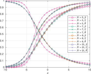
Figure 1. Numerical results for $\mathit{Ma}=1.4$ using Grad’s moment method with linearized ansatz

As a spectral method, its fast convergence can be clearly observed. Taking the results of $N=21$ as the reference solution, we find that the profiles computed by $N=7$ already have good agreement with the reference solution quantitatively. However, due to the lack of nonlinearity, the results of the five-moment system $N=5$ shows a significantly underestimated shock thickness. Below, in our experiments for the other four methods, the results of this method with $N=21$ will be used as the references solutions.

3.1.2. Grad’s moment method and hyperbolic moment method

For Mach number $1.4$, the temperature ratio is below $2.0$. Therefore convergence of both Grad’s moment method and the hyperbolic moment method can be expected. The numerical solutions for $N=5,7,9$ are provided in Figure 2. Two methods provide results with similar quality, due to the same ansatz (4) for the distribution function. Compared with Figure 1, the results for $N=5$ have been greatly improved, showing the superiority of a nonlinear ansatz for the distribution function. Comparing Figure 2a and Figure 2b, one can find that the hyperbolic moment method gives slightly better results than Grad’s moment method, as agrees with the observation in [13]. The underlying reason remains to be further studied. The simulation for the hyperbolic moment method is also faster than Grad’s moment method, since at each time step, we need to find the roots of a polynomial on each spatial grid to determine the time step according to the CFL condition.

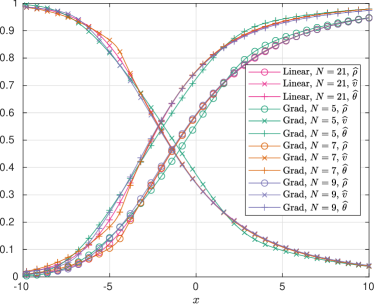
(a) Grad’s moment method

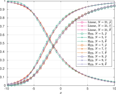
(b) Hyperbolic moment method

Figure 2. Numerical results for $\mathit{Ma}=1.4$ using Grad’s moment method and the hyperbolic moment method

3.1.3. Regularized moment method

The results of the regularized moment method with $N=5,7,9$ are shown in Figure 3, which also shows convergence as $N$ increases. Compared with Grad’s moment method and the hyperbolic moment method, the regularized moment method shows better results for $N=5$, since it essentially includes part of the information from the fifth moment. However, due to the second-order derivatives in the equations, much smaller time steps are required in the simulation, causing significantly longer computational time. Although this can be improved by using implicit treatment of these second-order derivatives, it can still be expected that longer computational time is needed than Grad’s moment method. The advantage of the regularized moment method is clearer in the high-dimensional case, where the number of moments is proportional to $N^{3}$, so that the regularized moment method can effectively reduce the degrees of freedom.

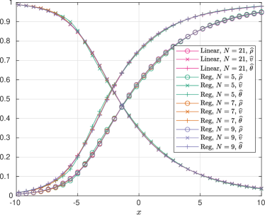
Figure 3. Numerical results for $\mathit{Ma}=1.4$ using regularized moment method

3.1.4. Quadrature-based moment method

For this method, we choose to use even number of moments in our tests as mentioned in Section 2.7. The cases tested in our simulation include $N=8$ and $12$, and we show the results in Figure 4. In general, QBMM can provide stable results, while the quality of approximation is not as good as previous methods. When $N=12$, we can still observe obvious difference between the QBMM result and the reference solution. The reason is likely to be the ansatz of QBMM, which consists of several Dirac delta functions that do not match the form of distribution functions in the shock structure.

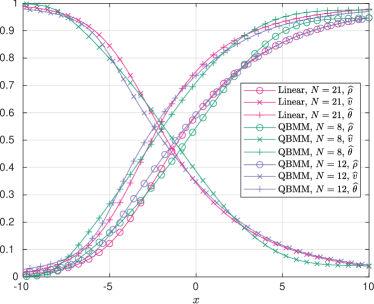
Figure 4. Numerical results for $\mathit{Ma}=1.4$ using quadrature-based moment method

3.2. Mach number $2.0$

The above numerical experiments show that the moment methods generally work well for Mach number $1.4$, despite the failure in some cases. However, when we increase the Mach number to $2.0$, the situation becomes much less optimistic. In this case, the density ratio is $1.6$ and temperature ratio is $3.44$. Since the temperature ratio exceeds $2$, the convergence issue of Grad-type methods (see [19]) will surface, resulting breakdown of the computation. The computational domain is set to be $[-30,30]$ for this much number. Our numerical results will be detailed in the following subsections.

3.2.1. Grad’s moment method with linearized ansatz

For Mach number $2.0$, choosing $\overline{\theta}=1$ quickly leads to breakdown of computation due to the divergence of (7) for fluid states behind the shock wave. This indicates that the manual selection of different parameters for different problems is essential in this method. By choosing $\overline{\theta}=2$ and $\overline{v}=\sqrt{3}\mathit{Ma}$, we can get convergent results, and the spectral method still shows its high efficiency (see Figure 5), and we will again use the result of $N=21$ as reference solution in the following numerical tests.

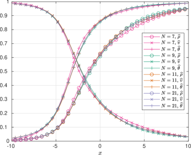
Figure 5. Numerical results for $\mathit{Ma}=2.0$ using Grad’s moment method with linearized ansatz

3.2.2. Grad’s moment method and hyperbolic moment method

Now Grad’s moment method faces problems coming from both hyperbolicity and convergence, and the instability of Grad’s moment method emerges. We tested $N=5,7,9,11$, and it turns out that only for $N=5$, we can achieve the steady state numerically from the discontinuous initial data. All other choices of $N$ end up with negative temperature in the computational process, which forces the simulation to terminate. In the numerical result for $N=5$ (Figure 6a), a discontinuity can be observed near $x=-7$, although it is smeared due to the dissipative numerical scheme, as is the notorious subshock phenomenon. Note that here we do not introduce any high-order schemes since these methods may introduce numerical instability. This discontinuity is known as an unphysical “subshock”, which is caused by the insufficient characteristic speed of the moment equations [33, 58]. Although using more moments can increase the characteristic speed, such a strategy is voided by the convergence problem, which will be detailed in Section 4.1.1.

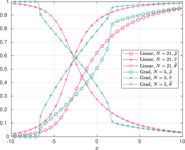
(a) Grad’s moment method

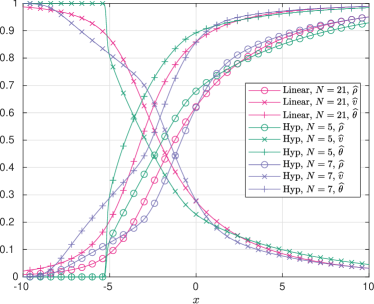
(b) Hyperbolic moment method

Figure 6. Numerical results for $\mathit{Ma}=2.0$ using Grad’s moment method and the hyperbolic moment method

As for the hyperbolic moment method, we can obtain stable numerical results for $N=5,7$, while for $N=9,11$, the computation breaks down due to the appearance of negative temperature, which agrees with the observation in [13]. This shows some advantages of the hyperbolic moment method due to the hyperbolicity fix. However, this does not overcome the convergence issue. The numerical results for $N=5,7$ are plotted in Figure 6b. Again, we can observe a subshock for $N=5$ near $x=-5$; when $N=7$, although the subshock no longer appears in the solution, the approximation of the shock structure is still unsatisfactory. In general, the performance of these moment methods is poorer than the case of $\mathit{Ma}=1.4$, owing to the stronger nonequilibrium inside the shock wave. Unfortunately, we are not able to further improve the result by increasing the number of moments with such an ansatz.

3.2.3. Regularized moment method

The regularized moment method suffers from the same issue as Grad’s moment method and the hyperbolic moment method. We tested $N=5,7,9,11$, and the only case that works is $N=5$, and we plot the results in Figure 7. Due to the regularization, the quality of approximation is better than Grad’s moment method, but the deviation is still obvious. Unfortunately, the regularization is not sufficient to stabilize the moment method when $N\geqslant 7$, and the simulation still fails by the ocurrence of negative temperature during the evolution.

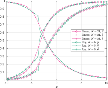
Figure 7. Numerical results for $\mathit{Ma}=2.0$ using regularized moment method

3.2.4. Quadrature-based moment method

The numerical results for the quadrature-based moment method are plotted in Figure 8, where the curves for $N=12$ and $14$ are provided. Figure 8 shows that the method shows the trend of convergence, but the efficiency is unsatisfactory, especially when compared with Figure 5. Even for $N=14$, the deviation from the reference solution is still obvious. Note that $N=14$ looks like a small number of degrees of freedom in the one-dimensional case, while in the three-dimensional case, the corresponding number of moments is $N(N+1)(N+2)/6=560$, and this number grows in the cubic manner as $N$ increases. Here we note that QBMM and related methods have achieved significant success in simulating disperse multiphase flows [28].

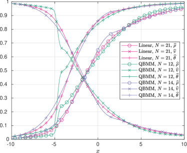
Figure 8. Numerical results for $\mathit{Ma}=2.0$ using quadrature-based moment method

4. Highest-moment-based moment method: One-dimensional case

The above numerical tests show intrinsic difficulties in computing shock structures using moment methods even for Mach number $2.0$ in the one-dimensional case, which does not look very high. The quadrature-based moment method looks like a possible solution, but its efficiency is lower than the Grad-type methods, and its generalization to three-dimensional case is nontrivial. Some untested methods such as the maximum entropy method may work better for high Mach numbers. Unfortunately, significant numerical difficulties exist in such computations. Is it possible to find alternative moment hierarchies as simple as Grad’s moment methods to deal with high-speed flows? We are going to explore such possibilities in this section. For simplicity, we will only address the one-dimensional case in this section. The more realistic three-dimensional case will be discussed later in Section 5.

4.1. Derivation of the moment equations

The derivation of the novel moment hierarchy in the one-dimensional case can be demonstrated in two steps. We will first propose an ansatz for the distribution function, and then apply the model-reduction technique in [12] to obtain moment systems.

4.1.1. Ansatz for the distribution function

Before writing down our ansatz of the distribution function, we would like to propose several principles that the ansatz must follow. In order to build reliable moment models to compute the shock structure for large Mach numbers, the ansatz must satisfy:

C1:

Any Maxwellian can be represented exactly by the ansatz.

C2:

The system does not require any parameters that cannot be determined by the moments in the system.

C3:

The ansatz converges to any linear combination of any Gaussians as the number of moments tends to infinity.

The first condition means that the Euler limit must be preserved. The second condition ensures that no additional parameters are introduced into the ansatz. The third condition takes into account the possible shapes of the distribution functions appearing in the shock structure. According to the Mott-Smith theory, [44], the distribution functions inside the shock wave can be well approximated by the linear combination of two Gaussians representing the fluid state in front of and behind the shock wave. Condition C3 is the one that Grad’s ansatz violates, especially when the temperature ratio exceeds $2$. We refer the readers to [19] for details on this convergence issue. Here we just briefly mention that given $\theta_{1}$ and $\theta_{2}$ satisfying $\theta_{1}>2\theta_{2}>0$, for any $v_{1},v_{2}\in\mathbb{R}$ and $\rho_{1},\rho_{2}\in\mathbb{R}_{+}$, we can always find a sufficiently small $\kappa>0$ such that Grad’s series (4) for the distribution function

(18) $$f(\xi)=(1-\kappa)\frac{\rho_{1}}{\sqrt{2\pi\theta_{1}}}\exp\left(-\frac{(\xi-v_{1})^{2}}{2\theta_{1}}\right)+\kappa\frac{\rho_{2}}{\sqrt{2\pi\theta_{2}}}\exp\left(-\frac{(\xi-v_{2})^{2}}{2\theta_{2}}\right)$$

diverges, since when $\kappa$ is small, the temperature $\theta$ of the above distribution function is close to $\theta_{2}$, so that $[f(\xi)]^{2}/\mathcal{M}_{0}(\xi)$ tends to infinity as $\xi\rightarrow\infty$, which violates the condition (10).

Despite the this drawback of Grad’s method, its simplicity and good approximability inspire us to use a similar form of the ansatz:

(19) $$f(x,\xi,t)=\sum_{\alpha=0}^{N-1}f_{\alpha}(x,t)\Theta(x,t)^{-\alpha/2}\mathit{He}_{\alpha}\left(\frac{\xi-V(x,t)}{\sqrt{\Theta(x,t)}}\right)\cdot\frac{1}{\sqrt{2\pi\Theta(x,t)}}\exp\left(-\frac{|\xi-V(x,t)|^{2}}{2\Theta(x,t)}\right).$$

The value of $V(x,t)$ will still be chosen as the velocity $v(x,t)$, which describes the center of the distribution function, so that $f_{1}\equiv 0$. However, to get convergence, we need to choose $\Theta(x,t)$ which can better reflect the decay rate in the tail of the distribution function, so that Condition C3 can be respected. By Condition C2, the quantity $\Theta(x,t)$ can only be constructed from the first $N$ moments. While Grad’s moment method only uses the second moment to find $\Theta$, we would like to consider using the highest moment to define $\Theta$, which better describes the behavior of the tail. Based on this idea, we can figure out the precise definition of $\Theta$ by Condition C1, meaning that $\Theta$ must equal $\theta$ for the equilibrium distribution function. For Maxwellians defined in (3), the highest moment ($(N-1)$th moment) is

$$\int_{\mathbb{R}}(\xi-v)^{N-1}\mathcal{M}(\xi)\,\mathrm{d}\xi=\left\{\begin{array}[]{ll}(N-2)!!\rho\theta^{(N-1)/2},&\text{if }N\text{ is odd},\\ 0,&\text{if }N\text{ is even}.\end{array}\right.$$

When $N$ is odd, we see that for Maxwellians,

$$\theta=\left(\frac{1}{(N-2)!!\rho}\int_{\mathbb{R}}(\xi-v)^{N-1}\mathcal{M}(\xi)\,\mathrm{d}\xi\right)^{2/(N-1)}.$$

Therefore, for any distribution function $f(\xi)$, we choose to define

(20) $$\Theta=\left(\frac{1}{(N-2)!!\rho}\int_{\mathbb{R}}(\xi-v)^{N-1}f(\xi)\,\mathrm{d}\xi\right)^{2/(N-1)},$$

so that when $f(\xi)$ happens to be a Maxwellian, the value of $\Theta$ coincides with $\theta$, and this Maxwellian can be exactly represented by the ansatz (19) with $f_{1}=f_{2}=\cdots=f_{N-1}=0$. When $N$ is even, the highest moment for Maxwellians equal zero, which does not provide any information for us to define $\Theta$. In this case, we can take the $(N-2)$th moment instead and define $\Theta$ by

$$\Theta=\left(\frac{1}{(N-3)!!\rho}\int_{\mathbb{R}}(\xi-v)^{N-2}f(\xi)\,\mathrm{d}\xi\right)^{2/(N-2)},$$

In this paper, we focus only on the case of odd $N$.

By choosing (20) in (4), we can get another constraint of the coefficients other than $f_{1}=0$. Taking the $(N-1)$th moment for (4), we have

$$\int_{\mathbb{R}}(\xi-v)^{N-1}f(\xi)\,\mathrm{d}\xi=\sum_{\begin{subarray}{c}\alpha=0\\ \alpha\text{ is even}\end{subarray}}^{N-1}\frac{(N-1)!}{(N-1-\alpha)!!}f_{\alpha}\Theta^{(N-1-\alpha)/2}.$$

Combining the above equation and (20), one finds that

(21) $$\sum_{\begin{subarray}{c}\alpha=2\\ \alpha\text{ is even}\end{subarray}}^{N-1}\frac{f_{\alpha}\Theta^{(N-1-\alpha)/2}}{(N-1-\alpha)!!}=0,$$

where we have used the fact that $\rho=f_{0}$. This also confirms that Condition C2 holds for this ansatz, since there are essentially only $N$ parameters in the ansatz (19), which can be fully determined by the $N$ moments.

The verification of Condition C3 is also straightforward. Given the sum of a number of Gaussians

$$f(\xi)=\sum_{k=1}^{K}\frac{\rho_{k}}{\sqrt{2\pi\theta_{k}}}\exp\left(-\frac{(\xi-v_{k})^{2}}{2\theta_{k}}\right),$$

we have

$$\int_{\mathbb{R}}(\xi-v)^{N-1}f(\xi)\,\mathrm{d}\xi=(N-2)!!\sum_{k=1}^{K}\rho_{k}Q_{k}(\theta_{k}),$$

where $Q_{k}(\cdot)$ are monic polynomials of degree $(N-1)/2$:

$$Q_{k}(x)=\sum_{\begin{subarray}{c}\alpha=0\\ \alpha\text{ is even}\end{subarray}}^{N-1}\begin{pmatrix}N-1\\ \alpha\end{pmatrix}(v_{k}-v)^{\alpha}\frac{(N-2-\alpha)!!}{(N-2)!!}x^{(N-1-\alpha)/2}.$$

Without loss of generality, we assume $\theta_{1}\leq\theta_{2}\leq\cdots\leq\theta_{K}$. Then it can be directly verified that

$$\lim_{N\rightarrow+\infty}\left(\sum_{k=1}^{K}\frac{\rho_{k}}{\rho}P_{k}(\theta_{k})\right)^{2/(N-1)}=\theta_{K}.$$

This means for sufficiently large $N$, the slowest decay of the Gaussian can be captured, as ensures the convergence of the ansatz.

It is worth mentioning that such a choice of $\Theta$ can capture the tail of a much wider range of distribution functions. It can be shown that if the slowest decay of the tail behaves like $\exp\big{(}{-}\xi^{2}/(2\vartheta)\big{)}$, then when $N$ tends to infinity, the value of $\Theta$ always tends to $\vartheta$. This indicates that such a method is not specially designed for the shock structure problem. Rigorous analysis of the convergence and wider applications of this expansion are included in our ongoing works.

Based on this ansatz, we will apply the methodology introduced in [12] to obtain a hyperbolic system. The details will be introduced in the following section.

4.1.2. System for the coefficients

The reference [12] provides a general framework to derive hyperbolic reduced models from the kinetic equations. Our ansatz of the distribution function (4) fits this framework perfectly, so that we can directly follow the steps therein the derive the equations. The details are listed below:

• Compute time and spatial derivatives:

  $$\frac{\partial f}{\partial t} =\sum_{\alpha=0}^{N+1}\left(\frac{\partial f_{\alpha}}{\partial t}+\frac{\partial u}{\partial t}f_{\alpha-1}+\frac{1}{2}\frac{\partial\Theta}{\partial t}f_{\alpha-2}\right)\mathcal{H}_{\alpha}^{[\Theta(x,t)]}\left(\frac{\xi-v(x,t)}{\sqrt{\Theta(x,t)}}\right),$$

  $$\frac{\partial f}{\partial x} =\sum_{\alpha=0}^{N+1}\left(\frac{\partial f_{\alpha}}{\partial x}+\frac{\partial u}{\partial x}f_{\alpha-1}+\frac{1}{2}\frac{\partial\Theta}{\partial x}f_{\alpha-2}\right)\mathcal{H}_{\alpha}^{[\Theta(x,t)]}\left(\frac{\xi-v(x,t)}{\sqrt{\Theta(x,t)}}\right),$$

  where $f_{\alpha}$ is regarded as zero if $\alpha<0$ or $\alpha\geqslant N$, and

  $$\mathcal{H}_{\alpha}^{[\Theta(x,t)]}(c)=\Theta(x,t)^{-\alpha/2}\mathit{He}_{\alpha}(c)\cdot\frac{1}{\sqrt{2\pi\Theta(x,t)}}\exp\left(-\frac{c^{2}}{2}\right).$$

• Truncate the series:

  (22) $$\frac{\partial f}{\partial t} \approx\sum_{\alpha=0}^{N-1}\left(\frac{\partial f_{\alpha}}{\partial t}+\frac{\partial v}{\partial t}f_{\alpha-1}+\frac{1}{2}\frac{\partial\Theta}{\partial t}f_{\alpha-2}\right)\mathcal{H}_{\alpha}^{[\Theta(x,t)]}\left(\frac{\xi-v(x,t)}{\sqrt{\Theta(x,t)}}\right),$$

  (23) $$\frac{\partial f}{\partial x} \approx\sum_{\alpha=0}^{N-1}\left(\frac{\partial f_{\alpha}}{\partial x}+\frac{\partial v}{\partial x}f_{\alpha-1}+\frac{1}{2}\frac{\partial\Theta}{\partial x}f_{\alpha-2}\right)\mathcal{H}_{\alpha}^{[\Theta(x,t)]}\left(\frac{\xi-v(x,t)}{\sqrt{\Theta(x,t)}}\right).$$

  Here the step (23) does not exist in Grad’s moment method, as is the reason for the loss of hyperbolicity.

• Approximate the advection term: Define

  $$\mathcal{F}_{\alpha}=\frac{\partial f_{\alpha}}{\partial x}+\frac{\partial v}{\partial x}f_{\alpha-1}+\frac{1}{2}\frac{\partial\Theta}{\partial x}f_{\alpha-2}.$$

  Then

  (24) $$\begin{split}\xi\frac{\partial f}{\partial x}&\approx\sum_{\alpha=0}^{N-1}\mathcal{F}_{\alpha}\xi\mathcal{H}_{\alpha}^{[\Theta(x,t)]}\left(\frac{\xi-v(x,t)}{\sqrt{\Theta(x,t)}}\right)\\ &=\sum_{\alpha=0}^{N}[\Theta\mathcal{F}_{\alpha-1}+v\mathcal{F}_{\alpha}+(\alpha+1)\mathcal{F}_{\alpha+1}]\mathcal{H}_{\alpha}^{[\Theta(x,t)]}\left(\frac{\xi-v(x,t)}{\sqrt{\Theta(x,t)}}\right)\quad[\mathcal{F}_{-1}=\mathcal{F}_{N}=\mathcal{F}_{N+1}=0]\\ &\approx\sum_{\alpha=0}^{N-1}[\Theta\mathcal{F}_{\alpha-1}+v\mathcal{F}_{\alpha}+(\alpha+1)\mathcal{F}_{\alpha+1}]\mathcal{H}_{\alpha}^{[\Theta(x,t)]}\left(\frac{\xi-v(x,t)}{\sqrt{\Theta(x,t)}}\right)\quad[\mathcal{F}_{-1}=\mathcal{F}_{N}=0]\end{split}$$

• Approximate the collision term:

  $$\begin{split}\frac{1}{\tau}(\mathcal{M}-f)&=\frac{1}{\tau}\sum_{\alpha=0}^{+\infty}\left[\frac{1+(-1)^{\alpha}}{2}\frac{\rho}{\alpha!!}(\theta-\Theta)^{\alpha/2}-f_{\alpha}\right]\mathcal{H}_{\alpha}^{[\Theta(x,t)]}\left(\frac{\xi-v(x,t)}{\sqrt{\Theta(x,t)}}\right)\\ &\approx\frac{1}{\tau}\sum_{\alpha=0}^{N-1}\left[\frac{1+(-1)^{\alpha}}{2}\frac{\rho}{\alpha!!}(\theta-\Theta)^{\alpha/2}-f_{\alpha}\right]\mathcal{H}_{\alpha}^{[\Theta(x,t)]}\left(\frac{\xi-v(x,t)}{\sqrt{\Theta(x,t)}}\right),\end{split}$$

  where the temperature $\theta$ can be computed by

  (25) $$\theta=\frac{1}{\rho}\int_{\mathbb{R}}|\xi-v|^{2}f(\xi)\,\mathrm{d}\xi=\Theta+\frac{2f_{2}}{\rho}.$$

• Assemble all the terms and formulate the equations:

  (26) $$\begin{split}\frac{\mathrm{d}f_{\alpha}}{\mathrm{d}t}+\frac{\mathrm{d}v}{\mathrm{d}t}f_{\alpha-1}+\frac{1}{2}\frac{\mathrm{d}\Theta}{\mathrm{d}t}f_{\alpha-2}+\Theta\mathcal{F}_{\alpha-1}+(1-\delta_{N-1,\alpha})(\alpha+1)\mathcal{F}_{\alpha+1}\\ =\frac{1}{\tau}\left[\frac{1+(-1)^{\alpha}}{2}\frac{\rho}{\alpha!!}(\theta-\Theta)^{\alpha/2}-f_{\alpha}\right],\quad\forall\alpha=0,1,\cdots,N-1.\end{split}$$

The final moment equations are given in (26), together with the relations $f_{0}=\rho$, $f_{1}=0$ and (21)(25). For simplicity, we will refer to this method as the highest-moment-based moment method (HMBMM). In the following section, several properties of the HMBMM will be discussed.

4.2. Properties of the moment systems

By the derivation of the moment system, it can be expected that this moment hierarchy is more promising to get convergence to the Boltzmann equation for a wider class of problems. Below we will focus on some other properties of the equations, including its hyperbolicity, asymptotic limit, and the balance laws of the moments.

4.2.1. Hyperbolicity of moment equations

The hyperbolicity of HMBMM can be observed by rewriting the equations using matrices and vectors. Let $\boldsymbol{w}=(f_{0},v,f_{2},\cdots,f_{N-2},\Theta)^{T}$ be the vector of unknowns, and

$$\boldsymbol{\mathcal{H}}(\xi)=\left(\mathcal{H}_{0}^{[\Theta]}\left(\frac{\xi-v}{\sqrt{\Theta}}\right),\mathcal{H}_{1}^{[\Theta]}\left(\frac{\xi-v}{\sqrt{\Theta}}\right),\cdots,\mathcal{H}_{N-1}^{[\Theta]}\left(\frac{\xi-v}{\sqrt{\Theta}}\right)\right)^{T}$$

be the vector of basis functions. Then (22)(23) can be rewritten as

$$\frac{\partial f}{\partial t}\approx\boldsymbol{\mathcal{H}}(\xi)^{T}\mathbf{D}\frac{\partial\boldsymbol{w}}{\partial t},\qquad\frac{\partial f}{\partial x}\approx\boldsymbol{\mathcal{H}}(\xi)^{T}\mathbf{D}\frac{\partial\boldsymbol{w}}{\partial x},$$

where $\mathbf{D}$ is a certain square matrix depending on $\boldsymbol{w}$. Here the vector $\mathbf{D}\partial_{x}\boldsymbol{w}$ equals $(\mathcal{F}_{0},\cdots,\mathcal{F}_{N-1})$. Therefore (24) can be rewritten as

$$\xi\frac{\partial f}{\partial x}\approx\boldsymbol{\mathcal{H}}(\xi)^{T}\mathbf{M}\mathbf{D}\frac{\partial\boldsymbol{w}}{\partial x},$$

where the matrix $\mathbf{M}$ is tridiagonal:

$$\mathbf{M}=\begin{pmatrix}v&1\\ \Theta&v&2\\ &\Theta&v&3\\ &&\ddots&\ddots&\ddots\\ &&&\Theta&v&N-1\\ &&&&\Theta&v\end{pmatrix}.$$

Such a derivation shows that the moment system can be written as

$$\mathbf{D}\frac{\partial\boldsymbol{w}}{\partial t}+\mathbf{M}\mathbf{D}\frac{\partial\boldsymbol{w}}{\partial x}=\boldsymbol{\mathcal{S}},$$

where the right-hand side $\boldsymbol{\mathcal{S}}$ represents the collision term, which does not affect the hyperbolicity. This formula shows that the system is hyperbolic if $\mathbf{M}$ is real diagonalizable, which can be easily observed since the characteristic polynomial of $\mathbf{M}$ is

$$\det(\lambda\mathbf{I}-\mathbf{M})=\mathit{He}_{N}\left(\frac{\lambda-v}{\sqrt{\Theta}}\right),$$

and all the roots of the Hermite polynomial are real and distinct if $\Theta$ is positive, as implies the hyperbolicity of the moment equations. Compared with the hyperbolic moment equations introduced in Section 2.4, HMBMM is more nonlinear since the characteristic speeds involve $\Theta$, which is expressed by the highest moment.

4.2.2. Asymptotic limits

We would now like to check whether the Euler and Navier-Stokes limits can be preserved by this moment hierarchy. When $N=3$, it is easy to see that the equations are identical to Euler equations of one-dimensional velocity. Below we only consider the case $N=5$. The equations with more moments can be analyzed using the same technique.

For $N=5$, the moment equations (26) can be reformulated as

(27) $$\frac{\mathrm{d}f_{0}}{\mathrm{d}t}+f_{0}\frac{\partial v}{\partial x} =0,$$

$$f_{0}\frac{\mathrm{d}v}{\mathrm{d}t}+\Theta\frac{\partial f_{0}}{\partial x}+f_{0}\frac{\partial\Theta}{\partial x}+2\frac{\partial f_{2}}{\partial x} =0,$$

$$\frac{\mathrm{d}f_{2}}{\mathrm{d}t}+\frac{1}{2}f_{0}\frac{\mathrm{d}\Theta}{\mathrm{d}t}+(3f_{2}+\Theta f_{0})\frac{\partial v}{\partial x}+3\frac{\partial f_{3}}{\partial x} =0,$$

$$\frac{\mathrm{d}f_{3}}{\mathrm{d}t}+f_{2}\frac{\mathrm{d}v}{\mathrm{d}t}+\frac{1}{2}\Theta f_{0}\frac{\partial\Theta}{\partial x}-\Theta\frac{\partial f_{2}}{\partial x}+4f_{3}\frac{\partial v}{\partial x} =-\frac{f_{3}}{\tau},$$

$$\frac{1}{2}\frac{\mathrm{d}f_{2}}{\mathrm{d}t}-\frac{f_{3}}{\Theta}\frac{\mathrm{d}v}{\mathrm{d}t}-f_{2}\frac{\partial v}{\partial x}-\frac{\partial f_{3}}{\partial x} =-\frac{f_{2}}{2\tau}\left(1+\frac{f_{2}}{\Theta f_{0}}\right).$$

Note that we have used the relation (21) to eliminate the variable $f_{4}$. We would like to first show that the system preserves Euler and Navier-Stokes limits when $\tau$ is small. For any quantity $\varphi\in\{f_{0},v,f_{2},f_{3},\Theta\}$, we expand it in terms of $\tau$ as

$$\varphi=\varphi^{(0)}+\tau\varphi^{(1)}+\tau^{2}\varphi^{(2)}+\cdots.$$

By the fourth equation of (27), it is clear that $f_{3}^{(0)}=0$; and it can be seen from the last equation of (27) that

$$f_{2}^{(0)}\left(1+\frac{f_{2}^{(0)}}{\Theta^{(0)}f_{0}^{(0)}}\right)=0.$$

If $f_{2}^{(0)}=-f_{0}^{(0)}\Theta^{(0)}$, the equation (25) shows that the leading order of temperature is negative, as is a non-physical state. Therefore $f_{2}^{(0)}=0$. Thus the zeroth-order approximation of the above system can be written from the first three equations of (27):

(28) $$\frac{\mathrm{d}f_{0}}{\mathrm{d}t}+f_{0}\frac{\partial v}{\partial x} =0,$$

$$f_{0}\frac{\mathrm{d}v}{\mathrm{d}t}+\Theta\frac{\partial f_{0}}{\partial x}+f_{0}\frac{\partial\Theta}{\partial x} =0,$$

$$\frac{\mathrm{d}\Theta}{\mathrm{d}t}+2\Theta\frac{\partial v}{\partial x} =0,$$

which is exactly the Euler equations for one-dimensional physics.

To get the first-order limit, we adopt Chapman-Enskog expansion, so that

$$f_{0}^{(k)}=0,\quad v^{(k)}=0,\quad\Theta^{(k)}=0,\qquad\text{for all }k\geqslant 1.$$

By the fourth equation of (27), we see that

$$f_{3}^{(1)}=-\frac{1}{2}\Theta f_{0}\frac{\partial\Theta}{\partial x},$$

which gives the Fourier law for heat conduction. The last equation in (27) shows that $f_{2}^{(1)}=0$. Therefore the first-order asymptotic limit can be obtained by changing the last equation of (28) to

(29) $$\frac{\mathrm{d}\Theta}{\mathrm{d}t}+2\Theta\frac{\partial v}{\partial x}=\frac{3}{f_{0}}\frac{\partial}{\partial x}\left(\tau f_{0}\Theta\frac{\partial\Theta}{\partial x}\right),$$

which corresponds to the Navier-Stokes equations for one-dimensional physics.

When we solve Euler equations or Navier-Stokes equations numerically, most of the time, we do not use the forms of equations like (28) or (29). Instead, we prefer writing the equations in the form of conservation laws so that one can easily apply conservative numerical schemes. Such a form for this moment hierarchy will be explored in the next section.

4.2.3. Balance laws of the moments

For the convenience of numerical computation, we would like to write the moment systems in the form similar to (12), which requires us to define the moments

(30) $$M_{k}=\langle\xi^{k}f\rangle,\qquad k=0,1,\cdots,N-1.$$

For simplicity, again we only write down the equations for $N=4$. By the ansatz (19), we can establish the relation between the moments (30) and the variables $f_{0},v,f_{2},f_{3},\Theta$:

$$M_{0}=f_{0},\qquad M_{1}=vf_{0},\qquad M_{2}=f_{0}(v^{2}+\Theta)+2f_{2},$$

$$M_{3}=vf_{0}(v^{2}+3\Theta)+6(vf_{2}+f_{3}),\qquad M_{4}=f_{0}(v^{4}+6v^{2}\Theta+3\Theta^{2})+12v(vf_{2}+2f_{3}).$$

Thus the moment system (27) can be written as

$$\frac{\partial M_{0}}{\partial t}+\frac{\partial M_{1}}{\partial x} =0,$$

$$\frac{\partial M_{1}}{\partial t}+\frac{\partial M_{2}}{\partial x} =0,$$

$$\frac{\partial M_{2}}{\partial t}+\frac{\partial M_{3}}{\partial x} =0,$$

$$\frac{\partial M_{3}}{\partial t}+\frac{\partial M_{4}}{\partial x} =-\frac{1}{\tau}\frac{2M_{1}^{3}-3M_{0}M_{1}M_{2}+M_{0}^{2}M_{3}}{M_{0}^{2}},$$

$$\frac{\partial M_{4}}{\partial t}+\frac{\partial M_{5}}{\partial x}+60\left(\Theta f_{2}\frac{\partial v}{\partial x}-f_{3}\frac{\partial\Theta}{\partial x}\right) =-\frac{1}{\tau}\frac{2M_{1}^{4}-3M_{0}^{2}M_{2}^{2}+M_{0}^{3}M_{4}}{M_{0}^{3}},$$

where

$$M_{5}=\langle\xi^{5}f\rangle=vf_{0}(v^{4}+10v^{2}\Theta+15\Theta^{2})+20v^{2}(vf_{2}+3f_{3})+60\Theta f_{3}.$$

It is straightforward to verify that this system is equivalent to (27). The first three equations are the conservation laws of mass, momentum and energy, and the fourth equation is a balance law for the third moment. These four equations can be considered as “exact” since they can be obtained directly by taking moments of the Boltzmann-BGK equation. The last equation contains 1) the moment closure given by the defintion of $M_{5}$; 2) a non-conservative product $\Theta f_{2}\partial_{x}v-f_{3}\partial_{x}\Theta$, which helps maintain the hyperbolicity of the system. The non-conservative product ruins the form of balance law in the last equation, as can be considered as the compromise to obtain a hyperbolic structure.

Such a formulation can be generalized to the case of a larger $N$. The resulting $N$-moment system always includes three conservation laws, $N-4$ balance laws, and one equation that involves the moment closure and the hyperbolicity fix. Due to the exactness of the first $N-1$ equations, it can also be expect that the asymptotic limit can be well preserved if the last equation does not spoil the order of magnitude. Also, such a form is more suitable for numerical simulation. In our numerical method, a standard finite volume method with Lax-Friedrichs numerical flux is applied, and the non-conservative product in the last equation is discretized by simple central differences. The results will be reported in the next subsection.

4.3. Numerical results

We are going to show some numerical results for shock structure computations using HMBMM. Again we consider the Boltzmann-BGK equation with initial condition (17). Numerical results for Mach numbers $1.4$ and $2.0$ are plotted in Figure 9. For $\mathit{Ma}=1.4$, the quality of the solution is equally good as the hyperbolic moment method shown in Figure 2b. For $\mathit{Ma}=2.0$, the simulations for all the three cases $N=5,7,9$ are stable, and the results of $N=9$ almost coincide with the reference solution. More importantly, the convergence of the numerical solution as $N$ gets larger can be clearly observed from the numerical results.

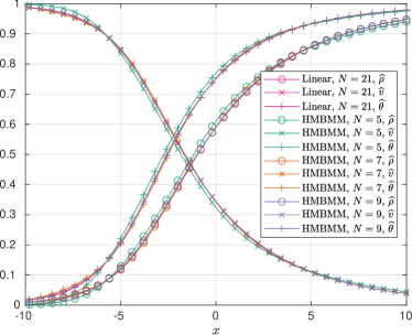
(a) $\mathit{Ma}=1.4$

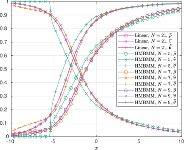
(b) $\mathit{Ma}=2.0$

Figure 9. Numerical results for $\mathit{Ma}=1.4$ and $\mathit{Ma}=2.0$

The numerical results show that HMBMM does not solve the subshock problem, since in front of the shock wave, when the distribution function is close to the Maxwellian, the value of $\Theta$ is close to the temperature $\theta$. Therefore the characteristic speeds of HMBMM are almost the same as those of Grad’s moment method or the hyperbolic moment method in this region. Nevertheless, for HMBMM, we can increase the number of moments to resolve the subshock issue.

To better understand the difference between the hyperbolic moment method and the highest-moment based moment method, we show the difference between $\theta$ and $\Theta$ in Figure 10, where $\widehat{\Theta}$ is defined by

$$\widehat{\Theta}(x)=\frac{\Theta(x)-\theta_{0}(-\infty)}{\theta_{0}(+\infty)-\theta_{0}(-\infty)}.$$

It can be observed that for most part of the shock wave, the value of $\Theta$ is greater than the temperature $\theta$, which better fits the tail of the distribution function. In fact, if the solution of the shock structure takes the form (18) everywhere, we should expect that $\Theta$ tends to $\theta_{0}(+\infty)$ everywhere as $N$ approaches infinity, which guarantees the convergence. Such a trend is validated by our numerical results, where $\Theta$ increases as $N$ increases. Figure 10b also explains why the temperature profile of $N=7$ shows significant deviation from the reference solution in the front part of the shock wave with $\mathit{Ma}=2$: when $N=7$, the parameter $\Theta$ is given by the sixth moment, using which one tends to underestimate the decay rate at the tail of the distribution function, leading to a relatively poor quality of approximation using (19).

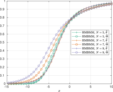
(a) $\mathit{Ma}=1.4$

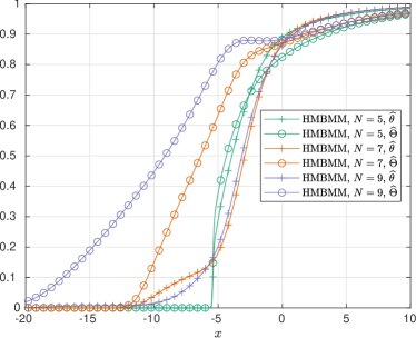
(b) $\mathit{Ma}=2.0$

Figure 10. Comparison between $\theta$ and $\Theta$ in one-dimensional HMBMM

5. Highest-moment-based moment method: Three-dimensional case

The methodology for the one-dimensional case can be generalized to the three-dimensional case without much difficulty, although the derivation is expected to be more tedious. Below we will only brief the idea of the generalization and provide the final moment equations, followed by some numerical tests to verify its capability in computing the high-speed shock structures.

5.1. Ansatz and the moment equations

In three-dimensional case, we can again adopt the ansatz of Grad’s moment method and only change the scaling parameter in the basis functions. Specifically, we assume

(31) $$\begin{split}f(\boldsymbol{x},\boldsymbol{\xi},t)&=\sum_{l=0}^{L-1}\sum_{m=-l}^{l}\sum_{n=0}^{N_{l}-1}f_{lmn}(\boldsymbol{x},t)[\Theta(\boldsymbol{x},t)]^{-(l+2n)/2}\times\\ &\quad p_{lmn}\left(\frac{\boldsymbol{\xi}-\boldsymbol{v}(\boldsymbol{x},t)}{\sqrt{\Theta(\boldsymbol{x},t)}}\right)\cdot\frac{1}{[2\pi\Theta(\boldsymbol{x},t)]^{3/2}}\exp\left(-\frac{|\boldsymbol{\xi}-\boldsymbol{v}(\boldsymbol{x},t)|^{2}}{2\Theta(\boldsymbol{x},t)}\right),\end{split}$$

where the parameters $L$ and $(N_{0},N_{1},\cdots,N_{L-1})$ specify the moments included in the moment system, and $p_{lmn}$ are orthogonal polynomials in the three-dimensional space. This choice of orthogonal polynomials follows [40, 17], which is based on the spherical coordinates in the three-dimensional space. The degree of the polynomial $p_{lmn}$ is $l+2n$, and the expressions are provided in Appendix A. Since $\boldsymbol{v}(\boldsymbol{x},t)$ is the velocity, the coefficients satisfy

$$f_{1m0}=0,\qquad m=-1,0,1.$$

In [18], the authors suggest choosing $N_{0}\geqslant N_{1}\geqslant\cdots\geqslant N_{L-1}$ so that the wall boundary conditions can be formulated appropriately. Some special choices of the parameters and the corresponding number of moments are given below:

• $L=2$, $N_{0}=2$, $N_{1}=1$: $5$ moments.

• $L=3$, $N_{0}=2$, $N_{1}=1$, $N_{2}=1$: $10$ moments.

• $L=3$, $N_{0}=N_{1}=2$, $N_{2}=1$: $13$ moments.

• $L=4$, $N_{0}=N_{1}=2$, $N_{2}=N_{3}=1$: $20$ moments.

• $L=4$, $N_{0}=3$, $N_{1}=N_{2}=2$, $N_{3}=1$: $26$ moments.

The key factor in this method is the choice of $\Theta$. The derivation is parallel to the one-dimensional case, which takes into account the conditions C1–C3. To fulfill Condition C3, we define $\Theta$ based on the following moment:

(32) $$\int_{\mathbb{R}^{3}}|\boldsymbol{\xi}-\boldsymbol{v}|^{2K}f(\boldsymbol{\xi})\,\mathrm{d}\boldsymbol{\xi},$$

where $K$ should be chosen as large as possible to best capture the decay of the tail. According to Condition C2, we need that the above quantity can be expressed by the moments included in the system. By the definition of $p_{lmn}$ given in (42), we can derive that

$$p_{00n}(\boldsymbol{c})=\sqrt{\frac{(2n)!!}{(2n+1)!!}}\sum_{i=0}^{n}(-1)^{i}\begin{pmatrix}n+1/2\\ n-i\end{pmatrix}\frac{|\boldsymbol{c}|^{2i}}{(2i)!!},\qquad n=0,1,\cdots,N_{0}-1.$$

Therefore using the variables $f_{lmn}$ appearing in (32), we can construct the moments (32) for all $K=0,1,\cdots,N_{0}-1$. Thus the greatest choice of $K$ is $N_{0}-1$. The expression of $\Theta$ should be formulated following Condition C1. For Maxwellians, the moment (32) is

(33) $$\int_{\mathbb{R}^{3}}|\boldsymbol{\xi}-\boldsymbol{v}|^{2(N_{0}-1)}\frac{\rho}{(2\pi\theta)^{3/2}}\exp\left(-\frac{|\boldsymbol{\xi}-\boldsymbol{v}|^{2}}{2\theta}\right)\,\mathrm{d}\boldsymbol{\xi}=(2N_{0}-1)!!\rho\theta^{2(N_{0}-1)}.$$

This inspires us to define $\Theta$ by

(34) $$\Theta=\left(\frac{1}{(2N_{0}-1)!!\rho}\int_{\mathbb{R}^{3}}|\boldsymbol{\xi}-\boldsymbol{v}|^{2(N_{0}-1)}f(\boldsymbol{\xi})\,\mathrm{d}\boldsymbol{\xi}\right)^{1/(2N_{0}-2)}.$$

By inserting (31) into (34), we obtain another constraint of the coefficients:

(35) $$\sum_{n=1}^{N_{0}-1}I_{n}\Theta^{N_{0}-1-n}f_{00n}=0,$$

where

$$I_{n}=\int_{\mathbb{R}^{3}}|\boldsymbol{v}|^{2(N_{0}-1)}p_{00n}(\boldsymbol{c})\cdot\frac{1}{(2\pi)^{3/2}}\exp\left(-\frac{|\boldsymbol{c}|^{2}}{2}\right)\,\mathrm{d}\boldsymbol{c},$$

which satisfies

$$I_{0}=(2N_{0}-1)!!,\qquad I_{n}=(n-N_{0})\sqrt{\frac{1}{(N_{0}-1)(N_{0}-1/2)}}I_{n-1},\quad\forall n>0.$$

Similar to the one-dimensional case, one can also prove that for the sum of any number of any Maxwellians, the ansatz (31) converges as $N\rightarrow\infty$. Here

$$N=\min\{l+2(N_{l}-1)\mid l=0,1,\cdots,L-1\},$$

which is the maximum degree of polynomials fully included in the ansatz. Thus Condition C3 is again fulfilled.

Based on this ansatz, the derivation of moment equations is similar to the 1D case. The general form of the final equations is

(36) $$\begin{split}&\frac{\mathrm{d}f_{lmn}}{\mathrm{d}t}+S_{lmn}+T_{lmn}=\\ &\qquad\frac{\Theta}{\mu}\sum_{l_{1}=0}^{L-1}\sum_{n_{1}=0}^{N_{l_{1}}-1}\sum_{l_{2}=0}^{L-1}\sum_{n_{2}=0}^{N_{l_{2}}-1}\sum_{\begin{subarray}{c}m_{1}=-l_{1},\cdots,l_{1}\\ m_{2}=-l_{2},\cdots,l_{2}\\ m_{1}+m_{2}=m\end{subarray}}A_{lmn}^{l_{1}m_{1}n_{1},l_{2}m_{2}n_{2}}\Theta^{(l+l_{1}-l_{2})/2+(n-n_{1}-n_{2})}f_{l_{1}m_{1}n_{1}}f_{l_{2}m_{2}n_{2}}.\end{split}$$

Here $S_{lmn}$ includes material derivatives of $\boldsymbol{v}$ and $\Theta$, and $T_{lmn}$ includes spatial derivatives of the coefficients. The form of the right-hand side comes from the quadratic form of the Boltzmann collision operator (2), and the coefficients $A_{lmn}^{l_{1}m_{1}n_{1},l_{2}m_{2}n_{2}}$ specifies the collision kernel. The precise form of the equations will be given in Appendix B.

The properties such as hyperbolicity and asymptotic limits can again be derived in the similar way to the one-dimensional case. Instead of carrying out the derivation with lengthy equations, here we just summarize the results briefly. The hyperbolicity of the equations can be observed by writing the equations in the following form:

$$\mathbf{D}\frac{\partial\boldsymbol{w}}{\partial t}+\sum_{j=1}^{3}\mathbf{M}_{j}\mathbf{D}\frac{\partial\boldsymbol{w}}{\partial x_{j}}=\boldsymbol{\mathcal{S}},$$

and it can be demonstrated that each $\mathbf{M}_{j}$ is symmetric, which implies the hyperbolicity. In fact, the system is symmetric hyperbolic, which can be observed by multiplying the above equation by $\mathbf{D}^{T}$. The asymptotic limits can be studied by Chapman-Enskog expansion. Actually, for systems with $5,10,13,20$ moments, since $N_{0}=2$, we can see from (34) that $\Theta=\theta$, and thus the ansatz (31) reduces to Grad’s ansatz, so that the corresponding moment system is identical to the hyperbolic moment equations with the same number of moments. This also indicates that the Euler limit and the Navier-Stokes limit can be preserved for sufficient number of moments. However, for the quadratic collision operators, preserving higher-order limits such as Burnett and super-Burnett is much more non-trivial just like in Grad’s moment methods. The balance-law form of the equations can also be derived by choosing moments $M_{lmn}=\langle\overline{p_{lmn}(\boldsymbol{\xi})}f(\boldsymbol{\xi})\rangle$, where we can find several equations including non-conservative terms to enforce the hyperbolicity.

5.2. Numerical method

To carry out the simulation of HMBMM, we take the idea of the approach proposed in [18] to carry out the simulation. For simplicity, we assume that a uniform grid with cell size $\Delta x$ is adopted, and at the $k$th time step, the distribution function on the $j$th grid is denoted by $F^{j,k}(\boldsymbol{\xi})$, which is defined as

$$F^{j,k}(\boldsymbol{\xi})=\sum_{l=0}^{L-1}\sum_{m=-l}^{l}\sum_{n=0}^{N_{l}-1}f_{lmn}^{j,k}\Psi^{j,k}(\boldsymbol{\xi}),$$

where

$$\Psi^{j,k}(\boldsymbol{\xi})=(\Theta^{j,k})^{-(l+2n)/2}\cdot p_{lmn}\left(\frac{\boldsymbol{\xi}-\boldsymbol{v}^{j,k}}{\sqrt{\Theta^{j,k}}}\right)\frac{1}{[2\pi\Theta^{j,k}]^{3/2}}\exp\left(-\frac{|\boldsymbol{\xi}-\boldsymbol{v}^{j,k}|^{2}}{2\Theta^{j,k}}\right).$$

Our discretization is based on the finite volume scheme:

(37) $$F_{*}^{j,k+1}(\boldsymbol{\xi})=F^{j,k}(\boldsymbol{\xi})-\frac{\Delta t}{\Delta x}\left[G_{+}^{j,k}(\boldsymbol{\xi})-G_{-}^{j,k}(\boldsymbol{\xi})\right]+\Delta t\sum_{l=0}^{L-1}\sum_{m=-l}^{l}\sum_{n=0}^{N_{l}-1}Q_{lmn}^{j,k}\Psi^{j,k}(\boldsymbol{\xi}),$$

where $Q_{lmn}^{j,k}$ is the right-hand side of (36) with $f_{l_{1}m_{1}n_{1}}$ and $f_{l_{2}m_{2}n_{2}}$ replaced by $f_{l_{1}m_{1}n_{1}}^{j,k}$ and $f_{l_{2}m_{2}n_{2}}^{j,k}$, respectively, and $G_{+}^{j,k}(\boldsymbol{\xi})$ and $G_{-}^{j,k}(\boldsymbol{\xi})$ are the numerical fluxes. To define the numerical fluxes, we introduce the projection operator $\mathcal{P}^{j,k}$, so that for any distribution function $g(\boldsymbol{\xi})$, the function $\mathcal{P}^{j,k}g$ has the form

(38) $$\mathcal{P}^{j,k}g(\boldsymbol{\xi})=\sum_{l=0}^{L-1}\sum_{m=-l}^{l}\sum_{n=0}^{N_{l}-1}\tilde{g}_{lmn}\Psi_{lmn}^{j,k}(\boldsymbol{\xi}),$$

which satisfies

$$\left\langle\overline{p_{lmn}\left(\frac{\boldsymbol{\xi}-\boldsymbol{v}^{j,k}}{\sqrt{\Theta^{j,k}}}\right)}g(\boldsymbol{\xi})\right\rangle=\left\langle\overline{p_{lmn}\left(\frac{\boldsymbol{\xi}-\boldsymbol{v}^{j,k}}{\sqrt{\Theta^{j,k}}}\right)}\mathcal{P}^{j,k}g(\boldsymbol{\xi})\right\rangle$$

for all $l=0,1,\cdots,L-1$, $m=-l,\cdots,l$ and $n=0,1,\cdots,N_{l}-1$. This operator can be regarded as “series truncation” for the expansion of $g$ using basis functions $\Psi_{lmn}^{j,k}$. With this operator, we can write down the numerical fluxes following the HLL scheme:

$$G_{+}^{j,k}(\boldsymbol{\xi}) =\mathcal{P}^{j,k}\left(\frac{\lambda_{R}^{j+1/2,k}\xi_{1}F^{j,k}(\boldsymbol{\xi})-\lambda_{L}^{j+1/2,k}\xi_{1}\mathcal{P}^{j,k}F^{j+1,k}(\boldsymbol{\xi})+\lambda_{R}^{j+1/2,k}\lambda_{L}^{j+1/2,k}[\mathcal{P}^{j,k}F^{j+1,k}(\boldsymbol{\xi})-F^{j,k}(\boldsymbol{\xi})]}{\lambda_{R}^{j+1/2,k}-\lambda_{L}^{j+1/2,k}}\right),$$

$$G_{-}^{j,k}(\boldsymbol{\xi}) =\mathcal{P}^{j,k}\left(\frac{\lambda_{R}^{j-1/2,k}\xi_{1}\mathcal{P}^{j,k}F^{j-1,k}(\boldsymbol{\xi})-\lambda_{L}^{j-1/2,k}\xi_{1}F^{j,k}(\boldsymbol{\xi})+\lambda_{R}^{j-1/2,k}\lambda_{L}^{j-1/2,k}[F^{j,k}(\boldsymbol{\xi})-\mathcal{P}^{j,k}F^{j-1,k}(\boldsymbol{\xi})]}{\lambda_{R}^{j-1/2,k}-\lambda_{L}^{j-1/2,k}}\right).$$

Here we apply the operator $\mathcal{P}^{j,k}$ to $F^{j\pm 1,k}$ before multiplying it by $\xi_{1}$, as follows the derivation of the equations detailed in Section 4.1.2. Note that $\mathcal{P}^{j,k}F^{j,k}=F^{j,k}$, which is why we omit this operator in front of $F^{j,k}$. Multiplying $\xi_{1}$ by a function with the form (38) can be implemented by the recursion relation of the basis functions:

$$\begin{split}&\xi_{1}\sum_{l=0}^{L-1}\sum_{m=-l}^{l}\sum_{n=0}^{N_{l}-1}\tilde{g}_{lmn}\Psi_{lmn}^{j,k}(\boldsymbol{\xi})\\ ={}&\sum_{l=0}^{L-1}\sum_{m=-l}^{l}\sum_{n=0}^{N_{l}-1}\Bigg{(}\sqrt{\frac{(l-m-1)(l-m)(n+l+1/2)}{2(2l-1)(2l+1)}}\Theta^{j,k}\tilde{g}_{l-1,m+1,n}-\sqrt{\frac{(l-m-1)(l-m)(n+1)}{2(2l-1)(2l+1)}}\tilde{g}_{l-1,m+1,n+1}\\ &\qquad-\sqrt{\frac{(l+m-1)(l+m)(n+l+1/2)}{2(2l-1)(2l+1)}}\Theta^{j,k}\tilde{g}_{l-1,m-1,n}+\sqrt{\frac{(l+m-1)(l+m)(n+1)}{2(2l-1)(2l+1)}}\tilde{g}_{l-1,m-1,n+1}\\ &\qquad-\sqrt{\frac{(l-m+1)(l-m+2)n}{2(2l+1)(2l+3)}}\Theta^{j,k}\tilde{g}_{l+1,m-1,n-1}+\sqrt{\frac{(l-m+1)(l-m+2)(n+l+3/2)}{2(2l+1)(2l+3)}}\tilde{g}_{l+1,m-1,n}\\ &\qquad+\sqrt{\frac{(l+m+1)(l+m+2)n}{2(2l+1)(2l+3)}}\Theta^{j,k}\tilde{g}_{l+1,m+1,n-1}-\sqrt{\frac{(l+m+1)(l+m+2)(n+l+3/2)}{2(2l+1)(2l+3)}}\tilde{g}_{l+1,m+1,n}\\ &\qquad+v_{1}^{j,k}\tilde{g}_{lmn}\Bigg{)}\Psi_{lmn}^{j,k}(\xi).\end{split}$$

The maximum characteristic speeds $\lambda_{L}^{j+1/2,k}$ and $\lambda_{R}^{j+1/2,k}$ are computed by

$$\lambda_{L}^{j+1/2,k}=\min\left\{0,\lambda_{\min}(\xi_{1}\mathcal{P}^{j,k}),\lambda_{\min}(\xi_{1}\mathcal{P}^{j+1,k})\right\},\quad\lambda_{R}^{j+1/2,k}=\max\left\{0,\lambda_{\max}(\xi_{1}\mathcal{P}^{j,k}),\lambda_{\max}(\xi_{1}\mathcal{P}^{j+1,k})\right\}.$$

Here $\lambda_{\min}$ and $\lambda_{\max}$ denote the minimum and maximum eigenvalues of the operators. Since the operator is invariant up to translation by $v_{1}^{j,k}$ and scaling by $\sqrt{\Theta^{j,k}}$, the eigenvalues have the form

$$\lambda_{\min}(\xi_{1}\mathcal{P}^{j,k})=v_{1}^{j,k}+C_{\min}\sqrt{\Theta^{j,k}},\quad\lambda_{\max}(\xi_{1}\mathcal{P}^{j,k})=v_{1}^{j,k}+C_{\max}\sqrt{\Theta^{j,k}},$$

and the constants $C_{\min}$ and $C_{\max}$ can be precomputed by the power method. Finally, note that the expansion of the function $F_{*}^{j,k+1}(\boldsymbol{\xi})$ given in (37) does not satisfy the constraint (35). We need to compute $\boldsymbol{v}^{j,k+1}$ and $\Theta^{j,k+1}$ by

$$\boldsymbol{v}^{j,k+1}=\frac{\langle\boldsymbol{\xi}F_{*}^{j,k+1}(\boldsymbol{\xi})\rangle}{\langle F_{*}^{j,k+1}(\boldsymbol{\xi})\rangle},\qquad\Theta^{j,k+1}=\left(\frac{1}{(2N_{0}-1)!!}\frac{\left\langle|\boldsymbol{\xi}-\boldsymbol{v}^{j,k+1}|^{2(N_{0}-1)}F_{*}^{j,k+1}(\boldsymbol{\xi})\right\rangle}{\langle F_{*}^{j,k+1}(\boldsymbol{\xi})\rangle}\right)^{1/(2N_{0}-2)},$$

with which we can at last evolve the solution by $F^{j,k+1}(\boldsymbol{\xi})=\mathcal{P}^{j,k+1}F_{*}^{j,k+1}(\boldsymbol{\xi})$.

The only component missing in this approach is the implementation of the operator $\mathcal{P}^{j,k}$ in (38). If the function $g$ is already expressed in the form of

$$g(\boldsymbol{\xi})=\sum_{l,m,n}g_{lmn}\Psi_{lmn}^{j,k}(\boldsymbol{\xi}),$$

then the operator $\mathcal{P}^{j,k}$ is simply a direct truncation. Otherwise, the implementation of this operator follows the method introduced in [18]. Below we will omit the derivation and just briefly state the result by taking $\mathcal{P}^{j,k}F^{j+1,k}(\boldsymbol{\xi})$ as an example. Suppose

(39) $$\mathcal{P}^{j,k}F^{j+1,k}(\boldsymbol{\xi})=\sum_{l=0}^{L-1}\sum_{m=-l}^{l}\sum_{n=0}^{N_{l}-1}\tilde{F}_{lmn}^{j+1,k}\Psi_{lmn}^{j,k}(\boldsymbol{\xi}).$$

Then by defining

(40) $$\begin{gathered}V_{-1}^{j,k}=\frac{1}{2}(v_{1}^{j,k}-\mathrm{i}v_{2}^{j,k}),\quad V_{0}^{j,k}=v_{3}^{j,k},\quad V_{1}^{j,k}=-\frac{1}{2}(v_{1}^{j,k}+\mathrm{i}v_{2}^{j,k}),\\ \gamma_{lm}^{\mu}=\sqrt{\frac{[l+(2\delta_{1,\mu}-1)m+\delta_{1,\mu}][l-(2\delta_{-1,\mu}-1)m+\delta_{-1,\mu}]}{(2l-1)(2l+1)}},\end{gathered}$$

we can compute the coefficients in (39) as follows:

$$\tilde{F}_{lmn}^{j+1,k}=\sum_{i=0}^{l+2n}\varpi_{lmn}^{(i)},$$

where

$$\varpi_{lmn}^{(0)} =F_{lmn}^{j+1,k},$$

$$\varpi_{lmn}^{(i)} =\frac{1}{i}\sqrt{n(n+l+1/2)}(\Theta^{j,k}-\Theta^{j+1,k})\varpi_{l,m,n-1}^{(i-1)}-\frac{\sqrt{2}}{i}\sum_{\mu=-1}^{1}(V_{\mu}^{j,k}-V_{\mu}^{j+1,k})\times$$

$$\quad\left[(-1)^{\mu}\sqrt{n+l+1/2}\gamma_{l,m+\mu}^{-\mu}\varpi_{l-1,m+\mu,n}^{(k-1)}+\sqrt{n}\gamma_{-l-1,m+\mu}^{-\mu}\varpi_{l+1,m+\mu,n-1}^{(k-1)}\right],\quad i>0.$$

Details of the derivation can be found in [18].

In applications, we supplement the above first-order method by Heun’s method and linear reconstruction with MC limiter to achieve second order of accuracy, which is relatively straightforward and will not be introduced. The numerical tests will be introduced in the next subsection.

5.3. Numerical tests

Again we use the problem of shock structure to test HMBMM. For three-dimensional physics, we set the initial condition to be

(41) $$f(x,\boldsymbol{\xi},0)=\frac{n_{0}(x)}{(2\pi\theta_{0}(x))^{3/2}}\exp\left(-\frac{|\boldsymbol{\xi}-\boldsymbol{v}_{0}(x)|^{2}}{2\theta_{0}(x)}\right),$$

where

$$n_{0}(x)=\left\{\begin{array}[]{@{}ll}1,&\text{if }x<0,\\ \dfrac{4\mathit{Ma}^{2}}{\mathit{Ma}^{2}+3},&\text{if }x>0,\end{array}\right.\qquad\boldsymbol{v}_{0}(x)=\left\{\begin{array}[]{@{}ll}(\sqrt{5/3}\mathit{Ma},0,0)^{T},&\text{if }x<0,\\ \left(\sqrt{\dfrac{5}{3}}\dfrac{\mathit{Ma}^{2}+3}{4\mathit{Ma}},0,0\right)^{T},&\text{if }x>0,\end{array}\right.$$

$$\theta_{0}(x)=\left\{\begin{array}[]{@{}ll}1,&\text{if }x<0,\\ \dfrac{(5\mathit{Ma}^{2}-1)(\mathit{Ma}^{2}+3)}{16\mathit{Ma}^{2}},&\text{if }x>0.\end{array}\right.$$

Note that here the spatial variable $x$ remains to be one-dimensional, so that the advection term in the Boltzmann equation (1) reduces to $\xi_{1}\partial_{x}f$. The collision term is given by the inverse-power-law intermolecular potential, and we choose the power so that the viscosity index is $\omega=0.72$, which is often used to simulate the argon gas. More details about the collision term can be found in Appendix B, from which one can see that one unit length in the problem setting equals the mean free path for the flow in front of the shock wave. Here we consider two Mach numbers $\mathit{Ma}=3.8$ and $\mathit{Ma}=6.5$, for which the temperature ratios are $5.375$ and $14.07$, respectively. Both are larger than $2$ so that methods based on Grad’s ansatz fail to converge.

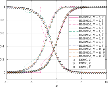
(a) Density, velocity and temperature

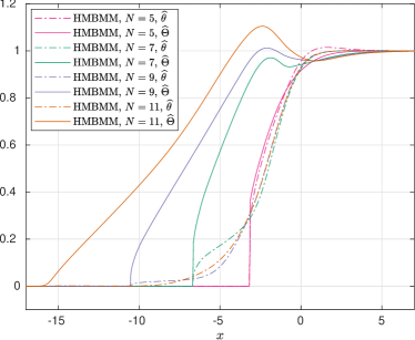
(b) Comparison between $\theta$ and $\Theta$

Figure 11. Numerical results for Mach number $3.8$

In our simulation, we adopt a second-order method implemented by linear reconstruction with the minmod limiter, so that the discontinuities (subshock) can be observed more clearly. A uniform grid with 2000 cells covering the range $[-30,30]$ is used. The DSMC solution, computed using Bird’s DSMC code [5, 6], is provided as a reference. In the ansatz (31), we choose $L$ and $N_{l}$ such that all polynomials $p_{lmn}$ of degree less than $N$ is included. Specifically, we set $L=N$ and $N_{l}=\lfloor(N+1-l)/2\rfloor$. For $\mathit{Ma}=3.8$, the results are shown in Figure 11. The left panel shows the curves for normalized density, velocity and temperature, where one can see that when $N=5,7$, the subshock still exists. When $N=9$, all the three curves for density, velocity, and temperature already have good agreement with the reference solution. However, by looking at Figure 11b, one can still observe the discontinuity around $x=-10$, while for $N=11$, the subshock is truly removed. In general, as the number of moments increases, the subshock moves in the direction of the front of the shock wave, and eventually disappears. Meanwhile, the discontinuity in the conservative quantities becomes smaller as $N$ increases. When the discontinuity is sufficiently small, we may consider the solution acceptable even if the unphysical subshock still exists.

Similar behavior can be observed for $\mathit{Ma}=6.5$, for which we plot the results in Figure 12. For $N=11$, although the subshock still exists, the location of the subshock is quite far from the center of the shock, so that the jumps in the first few moments are nearly negligible. Again the convergence is clearly seen as $N$ increases.

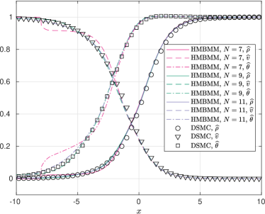
(a) Density, velocity and temperature

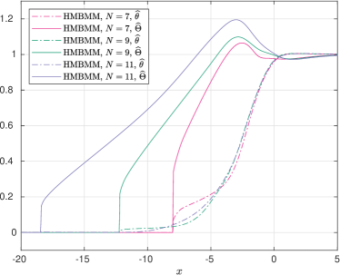
(b) Comparison between $\theta$ and $\Theta$

Figure 12. Numerical results for Mach number $6.5$

Some non-equilibrium variables, including the stress $\sigma_{xx}$ and the heat flux $q_{x}$, are plotted Figure 13, again with the DSMC results as references. These quantities are defined by

$$\sigma_{xx}=\int_{\mathbb{R}^{3}}(\xi_{1}-v_{1})^{2}f(\boldsymbol{\xi})\,\mathrm{d}\boldsymbol{\xi}-\rho\theta,\qquad q_{x}=\frac{1}{2}\int_{\mathbb{R}^{3}}|\boldsymbol{\xi}-\boldsymbol{v}|^{2}(\xi_{1}-v_{1})f(\boldsymbol{\xi})\,\mathrm{d}\boldsymbol{\xi}.$$

It can be observed that the values for these quantities are greater for larger Mach numbers, and the locations of the discontinuities in these quantities are the same as the locations of the subshocks in equilibrium quantities. In both cases, the graphs support the convergence to the smooth solutions.

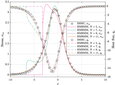
(a) Mach number $3.8$

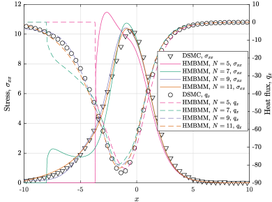
(b) Mach number $6.5$

Figure 13. Profiles of $\sigma_{xx}$ and $q_{x}$

We will now test the numerical efficiency of HMBMM. To this aim, we would like to reduce the number of grid cells while keeping the numerical solution acceptable. For both Mach numbers, we consider $N=11$ and run the codes for grids with $160$ cells and $1280$ cells. The numerical results are plotted in Figure 14. One can see that the two solutions are nearly identical, meaning that for $N=11$ and both Mach numbers, it is sufficient to use $160$ grid cells in our simulation. The machine for the computation has the CPU model “Intel^® Core™ i7-7600U” with clock frequency 2.8GHz. The code is run on a single thread with no parallelization. Some run-time data are given in Table 1. Note that our code is still to be optimized (it includes some duplicate computations of the numerical fluxes) and the efficiency is expected to be further improved by applying higher-order methods. We consider this computational cost as competitive since the quadratic collision operator is applied in the computation.

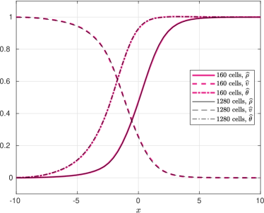
(a) $\mathit{Ma}=3.8$

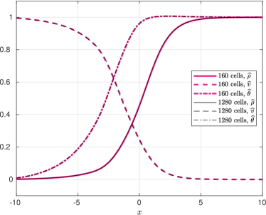
(b) $\mathit{Ma}=6.5$

Figure 14. Numerical results for different grid sizes

Table 1. Run-time data for shock structure computation with $160$ grid cells

	$\mathit{Ma}=3.8$		$\mathit{Ma}=6.5$
Number of time steps	4167		6796
Average time step	0.012		0.0074
Total computational time	1227.5s		2065.4s
Average computational time per time step	0.295s		0.304s

6. Applications beyond the plane shock structure problem

As mentioned previously, such an approach is not specially designed for the shock structure problem. We would therefore like to study the performance of the method in other problems. In this section, four more examples are presented. In the first two examples, we select problems where large temperature ratios do not exist in the initial condition, but emerge after the evolution of the flow. In the third example, the large temperature ratio is caused by the wall boundary conditions, and in the fourth example, a two-dimensional shock structure problem is studied to show the similar behavior as the one-dimensional case. As described in Appendix B, in all the simulations, the Knudsen number is $1.0$, meaning that the unit length equals the mean free path of the gas with unit density and temperature in equilibrium.

6.1. Colliding flows

We consider the one-dimensional flow whose initial condition is (41) with

$$\rho_{0}(x)=1,\qquad\boldsymbol{v}_{0}(x)=\left\{\begin{array}[]{ll}(1,0,0)^{T},&\text{if }x<0,\\ (-1,0,0)^{T},&\text{if }x>0,\end{array}\right.\qquad\theta_{0}(x)=1/3.$$

The two distribution functions in the initial data are plotted in Figure 15, which shows that the two Maxwellians have the same width, while there centers are separated. It can be expected that the fusion of these two Maxwellians can lead to a larger temperature that does not exist in the initial value.

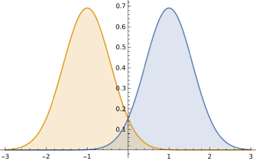
Figure 15. One-dimensional marginal distribution functions in the initial condition

In our computation, we set the domain to be $[-30,30]$, discretized by a uniform grid with $600$ cells. A second-order scheme is again applied in our numerical simulation. We present the numerical solutions for $N=5,7,9$, which are plotted in Figure 16. It is seen that a much higher temperature emerges in the middle of the flow such that the temperature ratio is well above $2.0$, which again fails the Grad-type methods. While for HMBMM, the simulations are stable, and the results look convergent as $M$ increases. Again, inside the shocks, the scaling factor $\Theta$ is mostly greater the temperature, so that the tail of the distribution function is better captured, as also stablizes the simulation. While $N=5$ (35-moment theory) cannot well capture the flow structure on both ends of the domain, we can safely increase $M$ to improve the quality of the solution. Note that for different $M$, the variable $\Theta$ stands for different moments, as explains why $\Theta$ does not look convergent in the figures. In the central part of the domain, the values of $\theta$ and $\Theta$ are relatively close to each other, since the higher density in this region causes higher collision rate, driving the distribution functions closer to Maxwellian, for which $\theta$ and $\Theta$ are equal.

The choice of $N$ in applications depends on the requirement of the accuracy. For this example, $N=6$ can already provide a good approximation. Note that it is important to keep $N$ small in simulations since the computational cost for the quadratic collision term usually increases quickly with respect to $N$. Being able to use a small $N$ can signficantly accelerate the simulation.

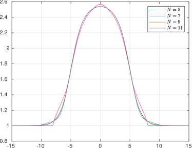
(a) $\rho$, $t=7.5$

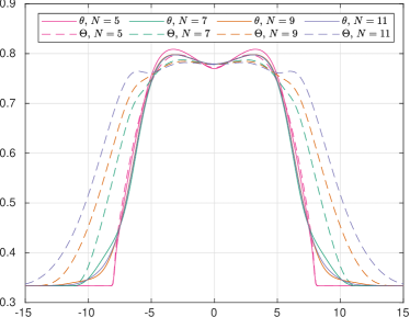
(b) $\theta$ and $\Theta$, $t=7.5$

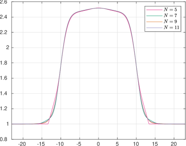
(c) $\rho$, $t=15$

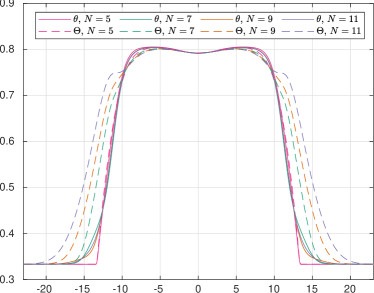
(d) $\theta$ and $\Theta$, $t=15$

Figure 16. Numerical results for the colliding flow

6.2. Cross-regime flows

Now we consider the shock tube problem with a large density ratio, for which the initial condition is (41) with

$$\rho_{0}(x)=\left\{\begin{array}[]{ll}65,&\text{if }|x|<6,\\ 1,&\text{if }|x|>6,\end{array}\right.\qquad\boldsymbol{v}_{0}(x)=0,\qquad\theta_{0}(x)=1.$$

In this example, while the Knusden number for $|x|>6$ is $1.0$, the central area $[-6,6]$ has the Knudsen number $1/65\approx 0.015$. Thus this problem can be considered as the interaction of the slip flow and the transitional flow. We again set the computationl domain to be $[-30,30]$ and divide it into $600$ uniform grid cells. The numerical results at $t=2.5$ and $t=5$ are presented in Figure 17.

For this problem, the high temperature ratio is generated by the high density ratio in the initial data. Therefore if we use the discrete velocity model to discretize the velocity space, we need to set a wide velocity domain to capture the high-temperature distribution functions and set a sufficiently small grid size to capture the low-temperature distribution functions. However, the nonlinearity in HMBMM can well adapt the ansatz to fit the above characters of the problem. The general feature of the numerical solution is similar to the previous example, such as the convergence with respect to $M$ and the relation between $\theta$ and $\Theta$, while this example better shows that HMBMM can simultaneously enjoy the advantages of the hydrodynamic equations and the spectral method at the same time: in the near-continuum regime, since the distribution function is close to Maxwellian, we need only a small number of moments even if the variation of the macroscopic quantities may be large; in the transitional regime, the method behaves like an adaptive spectral method which can efficiently capture the distribution function.

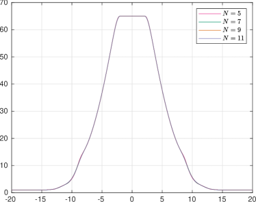
(a) $\rho$, $t=2.5$

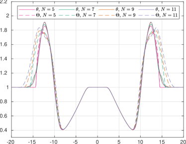
(b) $\theta$ and $\Theta$, $t=2.5$

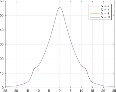
(c) $\rho$, $t=5$

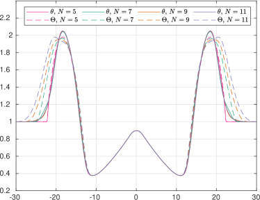
(d) $\theta$ and $\Theta$, $t=5$

Figure 17. Numerical results for the cross-regime flow

6.3. Fourier flow

In [19], the authors proposed another model problem that suffers from the loss of convergence for Grad’s moment method, which is the heat transfer between two parallel plates, known as the Fourier flow. Mathematically, this problem can be formulated by the Boltzmann equation

$$\frac{\partial f}{\partial t}+\xi_{1}\frac{\partial f}{\partial x}=\mathcal{S}[f],\qquad x\in(-L/2,L/2),\quad\boldsymbol{\xi}\in\mathbb{R}^{3}$$

with boundary conditions

$$f(-L/2,\boldsymbol{\xi},t)=\frac{\rho_{\mathrm{left}}(t)}{(2\pi\theta_{\mathrm{left}})^{3/2}}\exp\left(-\frac{|\boldsymbol{\xi}|^{2}}{2\theta_{\mathrm{left}}}\right)\text{ if }\xi_{1}>0,\quad f(L/2,\boldsymbol{\xi},t)=\frac{\rho_{\mathrm{right}}(t)}{(2\pi\theta_{\mathrm{right}})^{3/2}}\exp\left(-\frac{|\boldsymbol{\xi}|^{2}}{2\theta_{\mathrm{right}}}\right)\text{ if }\xi_{1}<0.$$

Here $\theta_{\mathrm{left}}$ and $\theta_{\mathrm{right}}$ are the temperatures of the left and right plates, respectively, and $\rho_{\mathrm{left}}(t)$ and $\rho_{\mathrm{right}}(t)$ are chosen such that

$$\int_{\mathbb{R}^{3}}\xi_{1}f(-L/2,\boldsymbol{\xi},t)\,\mathrm{d}\boldsymbol{\xi}=\int_{\mathbb{R}^{3}}\xi_{1}f(L/2,\boldsymbol{\xi},t)\,\mathrm{d}\boldsymbol{\xi}=0.$$

Such boundary conditions are known as diffuse reflection, where the distribution function of ingoing particles is given by a Maxwellian, whose center and variance are given by the velocity and temperature of the wall. For moment equations, the implementation of such boundary conditions follows the method introduced in [18], and its general idea is sketched in Appendix C.

In our test, we choose $L=5$ so that the effective Knudsen number is $0.2$ since we use the mean free path as the unit length. When $\theta_{\mathrm{left}}$ and $\theta_{\mathrm{right}}$ are close, the problem can be well approximated by linearizing the equations about a global Maxwellian. When linearized, the ansatz of HMBMM (19) becomes identical to Grad’s moment methods (4), and the results for Grad’s moment method in this linearized setting have been reported in some previous works (e.g. [60]). Therefore, here we choose a relatively large temperature ratio by setting

$$\theta_{\mathrm{left}}=1,\qquad\theta_{\mathrm{right}}=5.$$

According to [19], the steady state of this problem has a temperature ratio exceeding $2.0$, so that Grad’s moment method is expected to diverge. Our simulation starts with the initial condition

$$f(x,\boldsymbol{\xi},0)=\frac{1}{\sqrt{5\pi}}\exp\left(-\frac{|\boldsymbol{\xi}|^{2}}{5}\right),\qquad\forall x\in(-1,1),$$

and we evolve the solution until the steady state is reached. A uniform grid with $200$ cells is used for the spatial discretization.

Some numerical results with comparisons to the DSMC results are given in Figure 18. The temperature profiles confirm that the example involves temperature ratio greater than $2.0$, so that Grad’s moment method would fail to converge. In fact, as reported in [19], the steady-state solution of Grad’s moment method cannot be found in most cases. As for our method, due to the wall boundary conditions, the distribution functions on both ends of the domain are expected to be discontinuous, and thus we have used larger values of $N$ ($5$, $9$, $13$ and $17$) to show the convergence. It can be seen that under such a Knudsen number, the moment system with $N=9$ can already provide quite satisfactory results, and the curves for $N=13$ and $N=17$ are almost identical for equilibrium variables $\rho$ and $\theta$, while some tiny differences can still be observed in non-equilibrium quantities.

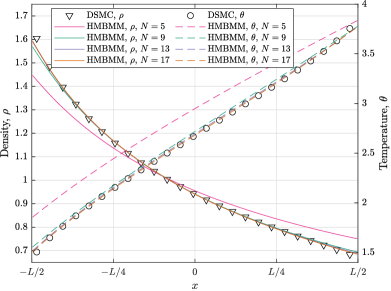
(a) $\rho$ and $\theta$

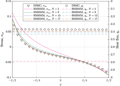
(b) $\sigma_{xx}$ and $q_{x}$

Figure 18. Numerical results for the Fourier flow

The values of $\Theta$ are shown in Figure 19. According to the boundary conditions, it is expected that when $N$ approaches infinity, the value of $\Theta$ should tend to $\max(\theta_{\mathrm{left}},\theta_{\mathrm{right}})=5.0$ everywhere. The reason is that the fat tail provided by the solid walls is expected to spread all over the domain, as is proven in [19] for the BGK collision model. Such a tendancy is observed in Figure 19, where we can see an obvious increase of $\Theta$ on all the points in the domain when $N$ increases. When the minimum value of $\Theta$ exceeds $2.5$, we can expect that the convergence of the expansion (31) can be achieved for all the distribution functions.

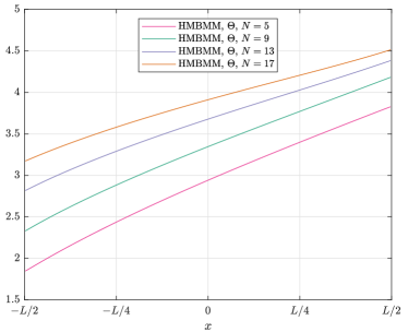
Figure 19. Parameter $\Theta$ for the Fourier flow

In most cases, for problems with wall boundary conditions, moment methods perform well mainly for the situation with relatively small Knudsen numbers due to the slow convergence rate of spectral expansions for discontinuous functions. We therefore suggest the use of this approach for effective Knudsen numbers below $0.5$, so that the region with strong discontinuity is restricted.

6.4. Hypersonic flow past a flat plate

In this example, we test the performance of HMBMM in a two-dimensional shock problem. We consider the case where the incoming flow with Mach number $5.0$ hits a flat plate, generating a bow shock in front of the plate. The setting of the problem is illustrated in Figure 20, where we assume that the incoming flow is parallel to the plate, so that we can impose the specular reflection boundary condition as illustrated in Figure 20, and thus only half of the domain needs to be simulated. In our simulation, we set the thickness of the plate to be $h=1$, and the size of the computational domain is given by $L=25$ and $H=20$. The length of the plate inside the computational domain is given by $\ell=10$. The incoming flow has density $1.0$ and temperature $1.0$, and inflow and outflow boundary conditions are imposed on the outer boundaries of the computational domain as indicated in Figure 20. The surface of the plate is assumed to be diffusive with temperature $\theta_{\mathrm{wall}}=1$. We refer the readers to Section 6.3 for the description of the diffuse reflection boundary conditions.

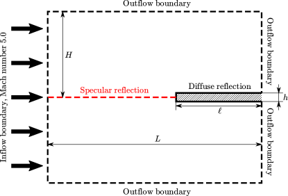
Figure 20. Settings of the two-dimensional shock problem

In our computation, a uniform grid with cell size $\Delta x=\Delta y=1/20$ is chosen for the spatial discretization. The numerical solutions for $\theta$ and $\Theta$ are shown in Figure 21 for $N=5,7,9,11$, where only part of the computation domain with interesting flow structure is plotted. In general, in spite of the large temperature ratio, the trend of convergence for the temperature plots can be observed, although we expect a larger $N$ to be used to get accurate flow states for such a large Knudsen number. Here we would like to draw the readers’ attention to the locations of the subshocks. When $N$ increases, the right panel of Figure 21 shows that the subshock gets farther away from the plate, which agrees with the one-dimensional case. For $N=5$ and $7$, the subshock can be clearly observed in the temperature plot, while for $N=7$, the temperature jump at the subshock is much weaker. For $N=9$ and $11$, although it is known that the subshocks exist, the jumps are already quite small and hardly observable in the temperature plots.

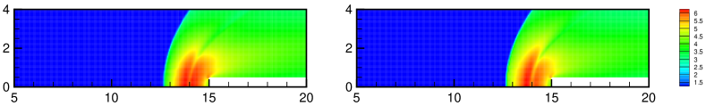
(a) $N=5$

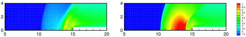
(b) $N=7$

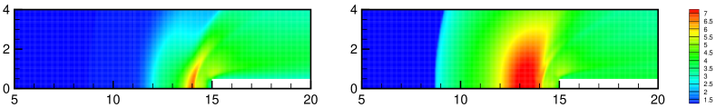
(c) $N=9$

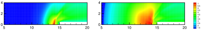
(d) $N=11$

Figure 21. Numerical solution for the two-dimensional shock problem. Left panel: $\theta$; Right panel: $\Theta$.

7. Discussion and conclusion

After witnessing that the shock structure problem disproves a number of moment hierarchies in the gas kinetic theory, we have built a variation of Grad’s moment method to face its challenge. The novel HMBMM takes into account the tail of the distribution function, as fixes the convergence issue of Grad’s moment method. Note that although HMBMM is not specially designed for the shock structure problem, our numerical tests show its capability in predicting the structures of high-speed shock waves. The HMBMM hierarchy constructs a more reliable bridge between hydrodynamic models and the kinetic equation, which may broaden the usage of the moment methods.

By the above numerical examples, we conclude that the HMBMM is mainly suitable for high-speed early transitional flows. In this flow regime, Grad’s method may fail due to its convergence problem, and the discrete velocity method (or Grad’s method with linearized ansatz) may require a large number of degrees of freedom to describe the distribution function. In this case, HMBMM has a chance to provide reasonable results using a relatively small number of moments. This is particularly useful when we need to use quadratic collision operator to capture the flow structure, since the computational cost of the quadratic collision operator usually increases at least quadratically with respect to the number of degrees of freedom. For highly nonequilibrium flows where a large number of degrees of freedom are needed to discretize the distribution function, the Fourier spectral method [47, 7, 31, 45, 25, 29] may be more efficient since the time complexity of such methods is significantly lower. This will happen when the gas is close to the regime of free molecules or when the shock is very strong.

Besides, for boundary value problems, due to the discontinuity in the distribution functions, the moment methods may not be able to well capture the structure of the boundary layers, which also restricts the use of HMBMM. Nevertheless, as a simple extension/stabilization of Grad’s moment method, it indicates that the nonlinear moment method without sophisticated closure still has a chance to work as a numerical solver of the Boltzmann equation, and we hope the idea of HMBMM can shed some light on the further development of the moment method. More works on the convergence theories of the moment methods, especially for boundary value problems, are currently going on.

Appendix A Definition of the polynomial $p_{lmn}$

In the ansatz of the three-dimensional distribution functions (31), the polynomials $p_{lmn}$ are three-dimensional orthogonal polynomials based on spherical coordinates. The definition is

(42) $$p_{lmn}(\boldsymbol{c})=\sqrt{\frac{2^{1-l}\pi^{3/2}n!}{\Gamma(n+l+3/2)}}L_{n}^{(l+1/2)}\left(\frac{|\boldsymbol{c}|^{2}}{2}\right)|\boldsymbol{c}|^{l}Y_{l}^{m}\left(\frac{\boldsymbol{c}}{|\boldsymbol{c}|}\right),\qquad l,n=0,1,\cdots,\quad m=-l,\cdots,l,$$

where $L_{n}^{(\alpha)}(\cdot)$ is the Laguerre polynomial

(43) $$L_{n}^{(\alpha)}(x)=\frac{x^{-\alpha}\exp(x)}{n!}\frac{\mathrm{d}^{n}}{\mathrm{d}x^{n}}[x^{n+\alpha}\exp(-x)],$$

and $Y_{l}^{m}(\cdot)$ is the spherical harmonics defined for $\boldsymbol{n}=(\sin\vartheta\cos\varphi,\sin\vartheta\sin\varphi,\cos\vartheta)^{T}$:

(44) $$Y_{l}^{m}(\boldsymbol{n})=\sqrt{\frac{2l+1}{4\pi}\frac{(l-m)!}{(l+m)!}}P_{l}^{m}(\cos\vartheta)\exp(\mathrm{i}m\varphi),$$

with $P_{l}^{m}(\cdot)$ being the associated Legendre functions:

$$P_{l}^{m}(x)=\frac{(-1)^{m}}{2^{l}l!}(1-x^{2})^{m/2}\frac{\mathrm{d}^{l+m}}{\mathrm{d}x^{l+m}}[(x^{2}-1)^{l}].$$

The polynomials $p_{lmn}(\cdot)$ satisfy the following orthogonality:

$$\int_{\mathbb{R}^{3}}p_{lmn}(\boldsymbol{c})p_{l^{\prime}m^{\prime}n^{\prime}}(\boldsymbol{c})\cdot\frac{1}{(2\pi)^{3/2}}\exp\left(-\frac{|\boldsymbol{c}|^{2}}{2}\right)\,\mathrm{d}\boldsymbol{c}=\delta_{ll^{\prime}}\delta_{mm^{\prime}}\delta_{nn^{\prime}}.$$

Note that $p_{lmn}(\cdot)$ is a complex-valued function satisfying

$$p_{lmn}(\boldsymbol{c})=(-1)^{m}\overline{p_{l,-m,n}(\boldsymbol{c})}.$$

Therefore in order that the distribution function (31) is real, the coefficients $f_{lmn}$ must satisfy

$$f_{lmn}=(-1)^{m}\overline{f_{l,-m,n}}.$$

This means that we only need to store about half of the coefficients appearing in (31) during the computation, but all the coefficients (except the ones with $m=0$) should be treated as complex numbers. One option to avoid complex numbers is to use real spherical harmonics defined using the real and imaginary parts of the complex spherical harmonics. However, such transformation will significantly complicate the calculation when deriving moment equations. Here we preserve the complex form as in some previous works of the author [17, 14], as is convenient for both derivation and numerical implementation.

Appendix B Definition of HMBMM equations

Here we provide supplementary clarifications of the three-dimensional equations (36). We will first define $S_{lmn}$ and $T_{lmn}$ on the left-hand side. The definition of $S_{lmn}$ is

(45) $$\begin{split}S_{lmn}&=-\sqrt{n(n+l+1/2)}\frac{\partial\Theta}{\partial t}f_{l,m,n-1}\\ &+\sqrt{2}\sum_{\mu=-1}^{1}\frac{\partial V_{\mu}}{\partial t}\left[(-1)^{\mu}\sqrt{n+l+1/2}\gamma_{l,m+\mu}^{-\mu}f_{l-1,m+\mu,n}-\sqrt{n}\gamma_{-l-1,m+\mu}^{-\mu}f_{l+1,m+\mu,n-1}\right],\end{split}$$

where $\gamma_{lm}^{\mu}$ and $V_{\mu}$ are defined in (40). The definition of $T_{lmn}$ requires to introduce the following complex differential operators:

$$\frac{\partial}{\partial X_{-1}}=\frac{\partial}{\partial x_{1}}+\mathrm{i}\frac{\partial}{\partial x_{2}},\qquad\frac{\partial}{\partial X_{0}}=\frac{\partial}{\partial x_{3}},\qquad\frac{\partial}{\partial X_{1}}=-\frac{\partial}{\partial x_{1}}+\mathrm{i}\frac{\partial}{\partial x_{2}},$$

which can be used to define

$$\begin{split}F_{lmn\mu}&=\frac{\partial f_{lmn}}{\partial X_{\mu}}+\sqrt{2}\sum_{\nu=-1}^{1}\frac{\partial V_{\nu}}{\partial X_{\mu}}\left[(-1)^{\nu}\sqrt{n+l+1/2}\gamma_{l,m+\nu}^{-\nu}f_{l-1,m+\nu,n}-\sqrt{n}\gamma_{-l-1,m+\nu}^{-\nu}f_{l+1,m+\nu,n-1}\right]\\ &-\sqrt{n(n+l+1/2)}\frac{\mathrm{d}\Theta}{\partial X_{\mu}}f_{l,m,n-1},\qquad l=0,1,\cdots,L-1,\quad m=-l,\cdots,l,\quad n=0,1,\cdots,N_{l}-1.\end{split}$$

If the indices of $F_{lmn\mu}$ are not in the range specified in the above equation, we regard its value as zero. Now we are ready to write down the formulas for $T_{lmn}$:

(46) $$T_{lmn}=\sum_{\mu=-1}^{1}\bigg{(}\frac{1}{2^{|\mu|}}\Big{[}\sqrt{2(n+l)+1}\gamma_{l,m-\mu}^{\mu}\Theta F_{l-1,m-\mu,n,\mu}-\sqrt{2(n+1)}\gamma_{l,m-\mu}^{\mu}F_{l-1,m-\mu,n+1,\mu}$$

$$\qquad+(-1)^{\mu}\gamma_{-l-1,m-\mu}^{\mu}(\sqrt{2(n+l)+3}F_{l+1,m-\mu,n,\mu}-\sqrt{2n}\Theta F_{l+1,m-\mu,n-1,\mu})\Big{]}\bigg{)}.$$

The derivation of the above equations can be found in [18].

The right-hand side of the equation (36) is determined by the collision kernel $B(\cdot,\cdot)$ in (2). For inverse-power-law intermolecular potentials, the coefficients $A_{lmn}^{l_{1}m_{1}n_{1},l_{2}m_{2}n_{2}}$ are all constants that can be precomputed, and $\mu=\mu_{0}\Theta^{\omega}$ with $\omega$ being a constant between $1/2$ and $1$. The computation of the coefficients $A_{lmn}^{l_{1}m_{1}n_{1},l_{2}m_{2}n_{2}}$ can be found in [14]. When simulating the shock structure, we choose to scale the coefficients such that

$$A_{200}^{200,000}+A_{200}^{000,200}=-1,$$

and we set

$$\mu_{0}=\sqrt{\frac{\pi}{2}}\frac{15}{(5-2\omega)(7-2\omega)},$$

so that the mean free path of the particles in the equilibrium state in front of the shock wave equals $1$.

Appendix C Diffuse reflection boundary condtions

In this appendix, we provide the sketch of the derivation of the diffuse reflection boundary conditions for the moment system. The details of the derivation is nearly identical to the procedure described in [18], except that the scaling factor $\theta$ (called $RT$ in [18]) needs to be replaced by $\Theta$ for HMBMM.

To ensure that the number of boundary conditions agrees with the number of characteristics pointing into the domain, we need that $N_{0}\geqslant N_{1}\geqslant\cdots\geqslant N_{l}$ in (31). Besides, for convenience, we assume that the solid wall has zero velocity. Under these assumptions, the derivation of the boundary conditions obeys the following rules:

• Let $\boldsymbol{n}$ be the outer unit normal vector on the boundary point $\boldsymbol{x}_{B}$. Then the boundary conditions have the form

  (47) $$\int_{\boldsymbol{\xi}\cdot\boldsymbol{n}<0}p(\boldsymbol{\xi})f(\boldsymbol{x}_{B},\boldsymbol{\xi},t)\,\mathrm{d}\boldsymbol{\xi}=\int_{\boldsymbol{\xi}\cdot\boldsymbol{n}<0}p(\boldsymbol{\xi})\frac{\rho_{\mathrm{wall}}(t)}{(2\pi\theta_{\mathrm{wall}})^{3/2}}\exp\left(-\frac{|\boldsymbol{\xi}|^{2}}{2\theta_{\mathrm{wall}}}\right)\,\mathrm{d}\boldsymbol{\xi},$$

  where $\theta_{\mathrm{wall}}$ denotes the temperature of the wall at point $x_{B}$, and $\rho_{\mathrm{wall}}(t)$ is given by

  (48) $$\rho_{\mathrm{wall}}(t)=\sqrt{\frac{2\pi}{\theta_{\mathrm{wall}}}}\int_{\boldsymbol{\xi}\cdot\boldsymbol{n}\geqslant 0}(\boldsymbol{\xi}\cdot\boldsymbol{n})f(\boldsymbol{x}_{B},\boldsymbol{\xi},t)\,\mathrm{d}\boldsymbol{\xi}.$$

  In both (47) and (48), the distribution function $f(\boldsymbol{x}_{B},\boldsymbol{\xi},t)$ is to be replaced by the truncated series (31), so that equations of the coefficients $f_{lmn}$ can be formed by (47).

• In (47), the function $p(\boldsymbol{\xi})$ must hold the form

  (49) $$p(\boldsymbol{\xi})=\sum_{l=0}^{L-1}\sum_{m=-l}^{l}\sum_{n=0}^{N_{l}-1}C_{lmn}p_{lmn}\left(\frac{\boldsymbol{\xi}-\boldsymbol{v}(\boldsymbol{x}_{B},t)}{\sqrt{\Theta(\boldsymbol{x}_{B},t)}}\right)$$

  for some constants $C_{lmn}$. Meanwhile, the polynomial $p(\boldsymbol{\xi})$ must satisfy

  (50) $$p(\boldsymbol{\xi})=-p(\boldsymbol{\xi}^{*}),\qquad\boldsymbol{\xi}^{*}=\boldsymbol{\xi}-2(\boldsymbol{\xi}\cdot\boldsymbol{n})\boldsymbol{n}.$$

  This condition means that the polynomial $p$ is symmetric about the wall.

• The functions satisfying both (49) and (50) form a finite dimensional linear space. The full set of boundary conditions at $\boldsymbol{x}_{B}$ is given by (47) with $p$ chosen as all the bases of this finite dimensional space.

Clearly $p(\boldsymbol{\xi})=\boldsymbol{\xi}\cdot\boldsymbol{n}$ is one of the polynomials satisfying both (49) and (50). For such a choice of $p$, the boundary condition (47) turns out to be

$$\boldsymbol{v}(\boldsymbol{x}_{B},t)\cdot\boldsymbol{n}=0,$$

meaning that the normal velocity of the gas is zero on the boundary.

References

- [1] M. R. A. Abdelmalik and E. H. van Brummelen, An entropy stable discontinuous Galerkin finite-element moment method for the Boltzmann equation, Comput. Math. Appl. 72 (2016), no. 8, 1988–1999.
- [2] by same author, Moment closure approximations of the Boltzmann equation based on -divergences, J. Stat. Phys. 164 (2016), no. 1, 77–104.
- [3] by same author, Error estimation and adaptive moment hierarchies for goal-oriented approximations of the Boltzmann equation, Comput. Methods Appl. Mech. Engrg. 325 (2017), 219–319.
- [4] J. D. Au, M. Torrilhon, and W. Weiss, The shock tube study in extended thermodynamics, Phys. Fluids 13 (2001), no. 8, 2423–2432.
- [5] G. A. Bird, Approach to translational equilibrium in a rigid sphere gas, Phys. Fluids 6 (1963), no. 10, 1518–1519.
- [6] by same author, Molecular gas dynamics and the direct simulation of gas flows, Oxford: Clarendon Press, 1994.
- [7] A. Bobylev and S. Rjasanow, Difference scheme for the Boltzmann equation based on the fast Fourier transform, Eur. J. Mech. B Fluids 16 (1997), no. 2, 293–306.
- [8] N. Böhmer and M. Torrilhon, Entropic quadrature for moment approximations of the Boltzmann-BGK equation, J. Comput. Phys. 401 (2020), 108992.
- [9] L. Boltzmann, Weitere studien über das wärmegleichgewicht unter gas-molekülen, Wiener Berichte 66 (1872), 275–370.
- [10] Z. Cai, Y. Fan, and R. Li, Globally hyperbolic regularization of Grad’s moment system in one dimensional space, Comm. Math. Sci. 11 (2013), no. 2, 547–571.
- [11] by same author, Globally hyperbolic regularization of Grad’s moment system, Comm. Pure Appl. Math. 67 (2014), no. 3, 464–518.
- [12] by same author, A framework on moment model reduction for kinetic equation, SIAM J. Appl. Math. 75 (2015), no. 5, 2001–2023.
- [13] by same author, Hyperbolic model reduction for kinetic equations, 2020, submitted.
- [14] Z. Cai, Y. Fan, and Y. Wang, Burnett spectral method for the spatially homogeneous Boltzmann equation, Computers & Fluids 200 (2020), 104456.
- [15] Z. Cai, R. Li, and Z. Qiao, Globally hyperbolic regularized moment method with applications to microflow simulation, Computers and Fluids 81 (2013), 95–109.
- [16] Z. Cai, R. Li, and Y. Wang, Numerical regularized moment method for high Mach number flow, Commun. Comput. Phys. 11 (2012), no. 5, 1415–1438.
- [17] Z. Cai and M. Torrilhon, Approximation of the linearized Boltzmann collision operator for hard-sphere and inverse-power-law models, J. Comput. Phys. 295 (2015), 617–643.
- [18] by same author, Numerical simulation of microflows using moment methods with linearized collision operator, J. Sci. Comput. 74 (2018), 336–374.
- [19] by same author, On the Holway-Weiss debate: Convergence of the Grad-moment-expansion in kinetic gas theory, Phys. Fluids 31 (2020), 126105.
- [20] Z. Cai and Y. Wang, Regularized 13-moment equations for inverse power law models, J. Fluid Mech. 894 (2020), A12.
- [21] G. Dimarco, R. Loubère, J. Narski, and T. Rey, An efficient numerical method for solving the Boltzmann equation in multidimensions, J. Comput. Phys. 353 (2018), 46–81.
- [22] W. Dreyer, Maximisation of the entropy in non-equilibrium, J. Phys. A: Math. Gen. 20 (1987), no. 18, 6505–6517.
- [23] Y. Fan and J. Koellermeier, Accelerating the convergence of the moment method for the Boltzmann equation using filters, J. Sci. Comput. 84 (2020), 1.
- [24] Y. Fan and R. Li, Globally hyperbolic moment system by generalized Hermite expansion, Scientia Sinica Mathematica 45 (2015), no. 10, 1635–1676.
- [25] F. Filbet, L. Pareschi, and T. Rey, On steady-state preserving spectral methods for homogeneous Boltzmann equations, Comptes Rendus Mathematique 353 (2015), no. 4, 309–314.
- [26] R. O. Fox, A quadrature-based third-order moment method for dilute gas-particle flows, J. Comput. Phys. 227 (2008), no. 12, 6313–6350.
- [27] by same author, Higher-order quadrature-based moment methods for kinetic equations, J. Comput. Phys. 228 (2009), no. 20, 7771–7791.
- [28] R. O. Fox, F. Laurent, and A. Vié, Conditional hyperbolic quadrature method of moments for kinetic equations, J. Comput. Phys. 365 (2018), 269–293.
- [29] I. M. Gamba, J. R. Haack, C. D. Hauck, and J. Hu, A fast spectral method for the Boltzmann collision operator with general collision kernels, SIAM J. Sci. Comput. 39 (2017), no. 14, B658–B674.
- [30] by same author, A fast spectral method for the Boltzmann collision operator with general collision kernels, SIAM J. Sci. Comput. 39 (2017), no. 14, B658–B674.
- [31] I. M. Gamba and S. H. Tharkabhushanam, Spectral-Lagrangian methods for collisional models of non-equilibrium statistical states, J. Comput. Phys. 228 (2009), no. 6, 2012–2036.
- [32] H. Grad, On the kinetic theory of rarefied gases, Comm. Pure Appl. Math. 2 (1949), no. 4, 331–407.
- [33] by same author, The profile of a steady plane shock wave, Comm. Pure Appl. Math. 5 (1952), no. 3, 257–300.
- [34] X. J. Gu and D. R. Emerson, A high-order moment approach for capturing non-equilibrium phenomena in the transition regime, J. Fluid Mech. 636 (2009), 177–216.
- [35] Z. Hu and Z. Cai, Burnett spectral method for high-speed rarefied gas flows, SIAM J. Sci. Comput. (2020), to appear.
- [36] Z. Hu, Z. Cai, and Y. Wang, Numerical simulation of microflows using Hermite spectral methods, SIAM J. Sci. Comput. 42 (2020), no. 1, B105–B134.
- [37] M. Junk, Domain of definition of Levermore’s five-moment system, J. Stat. Phys. 93 (1998), no. 5, 1143–1167.
- [38] G. Kitzler and J. Schröberl, A polynomial spectral method for the spatially homogeneous Boltzmann equation, SIAM J. Sci. Comput. 41 (2019), no. 1, B27–B49.
- [39] J. Koellermeier, R. P. Schaerer, and M. Torrilhon, A framework for hyperbolic approximation of kinetic equations using quadrature-based projection methods, Kin. Ret. Models 7 (2014), no. 3, 531–549.
- [40] K. Kumar, Polynomial expansions in kinetic theory of gases, Ann. Phys. 37 (1966), 113–141.
- [41] J. Laplante and C. P. T. Groth, Comparison of maximum entropy and quadrature-based moment closures for shock transitions prediction in one-dimensional gaskinetic theory, AIP Conference Proceedings 1786 (2016), 140010.
- [42] C. D. Levermore, Moment closure hierarchies for kinetic theories, J. Stat. Phys. 83 (1996), no. 5–6, 1021–1065.
- [43] C. Liu, K. Xu, Q. Sun, and Q. Cai, A unified gas-kinetic scheme for continuum and rarefied flows IV: Full Boltzmann and model equations, J. Comput. Phys. 314 (2016), 305–340.
- [44] H. M. Mott-Smith, The solution of the boltzmann equation for a shock wave, Phys. Rev. 82 (1951), 885–892.
- [45] C. Mouhot and L. Pareschi, Fast algorithms for computing the Boltzmann collision operator, Math. Comp. 75 (2006), no. 256, 1833–1852.
- [46] I. Müller and T. Ruggeri, Rational extended thermodynamics, second edition, Springer tracts in natural philosophy, vol. 37, Springer-Verlag, New York, 1998.
- [47] L. Pareschi and B. Perthame, A Fourier spectral method for homogeneous Boltzmann equations, Transport Theor. Stat. 25 (1996), no. 3–5, 369–382.
- [48] M. Sadr, M. Torrilhon, and M. H. Gorji, Gaussian process regression for maximum entropy distribution, 2019, submitted.
- [49] N. Sarna, J. Giesselmann, and M. Torrilhon, Convergence analysis of Grad’s Hermite expansion for linear kinetic equations, SIAM J. Numer. Anal. 58 (2020), no. 2, 1164–1194.
- [50] N. Sarna, H. Kapadia, and M. Torrilhon, Simultaneous-approximation-term based boundary discretization for moment equations of rarefied gas dynamics, J. Comput. Phys. 407 (2020), 109243.
- [51] R. P. Schaerer, P. Bansal, and M. Torrilhon, Efficient algorithms and implementations of entropy-based moment closures for rarefied gases, J. Comput. Phys. 340 (2017), 138–159.
- [52] R. P. Schaerer and M. Torrilhon, The 35-moment system with the maximum-entropy closure for rarefied gas flows, Eur. J. Mech. B - Fluids 64 (2017), 30–40.
- [53] H. Struchtrup, Derivation of 13 moment equations for rarefied gas flow to second order accuracy for arbitrary interaction potentials, Multiscale Model. Simul. 3 (2005), no. 1, 221–243.
- [54] H. Struchtrup and M. Torrilhon, Regularization of Grad’s 13 moment equations: Derivation and linear analysis, Phys. Fluids 15 (2003), no. 9, 2668–2680.
- [55] P. L. Tallec and J. P. Perlat, Numerical analysis of Levermore’s moment system, Rapport de recherche 3124, INRIA Rocquencourt, March 1997.
- [56] M. Yu. Timokhin, Ye. A. Bondar, A. A. Kokhanchik, M. S. Ivanov, I. E. Ivanov, and I. A. Kryukov, Study of the shock wave structure by regularized Grad’s set of equations, Phys. Fluids 27 (2015), no. 3, 037101.
- [57] M. Yu. Timokhin, H. Struchtrup, A. A. Kokhanchik, and Ye. A. Bondar, Different variants of R13 moment equations applied to the shock-wave structure, Phys. Fluids 29 (2017), 037105.
- [58] M. Torrilhon, Characteristic waves and dissipation in the 13-moment-case, Continuum Mech. Thermodyn. 12 (2000), no. 5, 289–301.
- [59] by same author, Hyperbolic moment equations in kinetic gas theory based on multi-variate Pearson-IV-distributions, Commun. Comput. Phys. 7 (2010), no. 4, 639–673.
- [60] by same author, Convergence study of moment approximations for boundary value problems of the Boltzmann-BGK equation, Commun. Comput. Phys. 18 (2015), no. 3, 529–557.
- [61] M. Torrilhon and H. Struchtrup, Regularized 13-moment equations: shock structure calculations and comparison to Burnett models, J. Fluid Mech. 513 (2004), 171–198.
- [62] J. C. Wheeler, Modified moments and Gaussian quadratures, Rocky Mountain J. Math. 4 (1974), no. 2, 287–296.
- [63] L. Wu, C. White, T. Scanlona, J. Reese, and Y. Zhang, Deterministic numerical solutions of the Boltzmann equation using the fast spectral method, J. Comput. Phys. 250 (2013), 27–52.
- [64] C. Yuan and R. O. Fox, Conditional quadrature method of moments for kinetic equations, J. Comput. Phys. 230 (2011), no. 22, 8126–8246.
- [65] C. Yuan, F. Laurent, and R. O. Fox, An extended quadrature method of moments for population balance equations, J. Aerosol Sci. 51 (2012), 1–23.
- [66] W. Zhao, W.-A. Yong, and L.-S. Luo, Stability analysis of a class of globally hyperbolic moment system, Commun. Math. Sci. 15 (2017), no. 3, 609–633.