Sound Event Localization and Detection Using
Activity-Coupled Cartesian DOA Vector and RD3net

Abstract

Our systems submitted to the DCASE2020 task 3: Sound Event Localization and Detection (SELD) are described in this report. We consider two systems: a single-stage system that solve sound event localization (SEL) and sound event detection (SED) simultaneously, and a two-stage system that first handles the SED and SEL tasks individually and later combines those results. As the single-stage system, we propose a unified training framework that uses an activity-coupled Cartesian DOA vector (ACCDOA) representation as a single target for both the SED and SEL tasks. To efficiently estimate sound event locations and activities, we further propose RD3Net, which incorporates recurrent and convolution layers with dense skip connections and dilation. To generalize the models, we apply three data augmentation techniques: equalized mixture data augmentation (EMDA), rotation of first-order Ambisonic (FOA) singals, and multichannel extension of SpecAugment. Our systems demonstrate a significant improvement over the baseline system.

Index Terms—  DCASE2020, Sound event localization and detection, ACCDOA, RD3Net

1 Introduction

Sound event localization and detection (SELD) is the task of identifying both the direction of arrival (DOA) and the type of sound. A number of methods have been tackling this challenging problem by decomposing tasks into several subtasks: the estimation of the number of sources, DOA estimation, and sound event detection (SED). Although this simplifies the SELD problem and therefore could improve the performance of each task, it also increases system complexity and computational cost. Here, we consider both the single- and two-stage systems. The single-stage system solve both SED and SEL task simultaneously using an activity-coupled Cartesian DOA vector (ACCDOA) representation. ACCDOA assigns an audio event activity to the length of a corresponding Cartesian DOA vector. On the other hand, the two-stage system first handles the SED as a frame wise classification problem and then combines with the DOA estimation.

2 System

In this section, we first give an overview of our two systems, namely, the ACCDOA (single-stage) system and the two-stage system. Then we explain the parts of our pipelines: the features, data augmentation, network architecture, and loss function.

2.1 System overview

A schematic flow of the ACCDOA system is shown in Fig. 1. Two data augmentation techniques are applied to input signals prior to the feature extraction while one data augmentation technique exploiting multichannel information in the feature domain is performed after the feature extraction. Finally, the network outputs frame-wise ACCDOA vectors for 14 sound events. The magnitude of the vectors corresponds to the probability of each sound event activity while the direction of the vectors points toward the location of each source. The model using the ACCDOA representation is trained to minimize the distance between the estimated and the target coordinates.

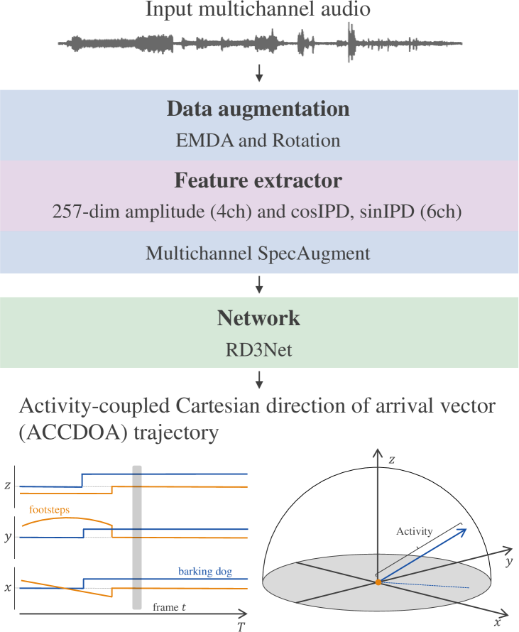
Figure 1: Illustration of our ACCDOA system.

The two-stage system is inspired by the work in [1]. This is characterized by three ideas: training only the SED branch, transferring a part of the network parameters from the SED branch to the DOA estimation branch, and training the DOA estimation branch. The data augmentation techniques, the features, and the network used in the system are exactly the same as the ones in the ACCDOA system.

2.2 Feature

Multichannel amplitude spectrograms and inter-channel phase differences (IPDs) are used as frame-wise features. Here, ${\rm IPD}_{t,f,p,q}=\angle{x}_{t,f,p}-\angle{x}_{t,f,q}$ is computed from the short-time Fourier transform (STFT) coefficients $x_{t,f,p}$ and $x_{t,f,q}$, where $t,f,p,$ and $q$ denote the time frame, the frequency bin, the microphone channel $p$, and the channel $q$, respectively. We fix $p=0$ to compute relative IPDs between all the other channels, $q$. Since the input consists of four channel signals, we can extract four amplitude spectrograms and three IPDs.

2.3 Data augmentation

To promote the generalization of the model, we exploit the following data augmentation techniques during the training.

• EMDA: As described in [2, 3], we apply the equalized mixture data augmentation (EMDA) method where up to two audio events are mixed with random amplitudes, delays, and the modulation of frequency characteristics, i.e. equalization.

• Rotation: We also adopt the spatial augmentation method in [4]. It rotates the training data represented in the first order Ambisonic (FOA) format and allows us to increase the numbers of DOA labels without losing the physical relationships between steering vectors and observations. We consider eight rotation patterns for azimuth $\phi$ and elevation $\theta$: $(\phi^{\prime},\theta^{\prime})=(\phi,\theta),(-\phi,\theta),(\phi+\pi,\theta),(-\phi+\pi,\theta),(\phi,-\theta),(-\phi,-\theta),(\phi+\pi,-\theta),(-\phi+\pi,-\theta)$.

• Multichannel SpecAugment: We propose a multichannel version of SpecAugment in [5, 6]. In addition to the time-frequency hard masking schemes applied on amplitude spectrograms, we also extend it to the channel dimension. The target channel for the channel masking, $c_{0}$, is chosen from $[0,C)$ where $C$ denotes the number of microphone channels. For the IPD features, instead of multiplying a mask value by the original value, the original values are replaced with random values, where the values are sampled from a uniform distribution ranging from 0 to $2\pi$.

2.4 Network architecture

As the network architecture, we adopt the D3Net architecture [7], which has shown the state-of-the-art performance in music source separation. The adaptation to the SELD problem includes three modifications. First, we omit dense blocks in the up-sampling path because high frame-rate prediction is not necessary for the SELD problem. Second, we replaced with GRU cells only in the bottleneck part. Third, the batch normalization is replaced with the network deconvolution [8]. We call this architecture RD3Net; the architecture is illustrated in Figure 2.

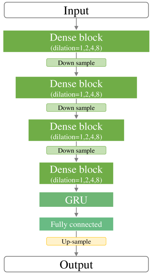
Figure 2: Illustration of RD3Net architecture.

2.5 Loss function

In the ACCDOA system, we solve the multi-output regression with a mean square error (MSE) loss. In the other system using the two-stage training scheme, we use a binary cross entropy (BCE) for the SED classification task and a masked MSE for the DOA regression task [1]. The latter is based on an MSE masked with the ground truth activations of each class, hence not contributing to the training when the corresponding sound event is not active.

2.6 Post-processing

During the inference, we split the 60 seconds inputs into shorter segments with overlap, process each segment, and average the results of overlapped frames. To further improve the performance, we conduct a post-processing with the following procedure: rotating the FOA data, estimating the ACCDOA vectors, rotating the vectors back, and averaging the vectors of different rotation patterns. Similar to section 2.3, we consider eight rotations.

2.7 Model ensemble

Table 1: Ensemble configuration.

Name	# of models	Base system
Ensemble 1	4	ACCDOA w/ RD3Net $\times$3
		Two-stage w/ RD3Net
Ensemble 2	5	ACCDOA w/ RD3Net $\times$3
		Two-stage w/ RD3Net, CRNN
Ensemble 3	5	ACCDOA w/ RD3Net $\times$3
		Two-stage w/ RD3Net $\times$2

Table 2: SELD performance of our systems evaluated using joint localization/detection metrics for the development set.

		Validation split				Testing split
Submission label	System	${LE}_{CD}$	${LR}_{CD}$	${ER}_{20^{\circ}}$	${F}_{20^{\circ}}$	${LE}_{CD}$	${LR}_{CD}$	${ER}_{20^{\circ}}$	${F}_{20^{\circ}}$
-	Baseline FOA	$23.5^{\circ}$	62.0	0.72	37.7	$22.8^{\circ}$	60.7	0.72	37.4
-	ACCDOA w/ CRNN	$7.8^{\circ}$	79.9	0.34	77.2	$8.9^{\circ}$	73.8	0.40	70.5
-	Two-stage w/ RD3Net	$8.6^{\circ}$	86.2	0.29	80.4	$9.7^{\circ}$	78.2	0.38	73.0
Shimada_SONY_task3_1	ACCDOA w/ RD3Net	$7.0^{\circ}$	87.0	0.24	84.4	$7.9^{\circ}$	80.5	0.32	76.8
Shimada_SONY_task3_2	Ensemble 1	$6.3^{\circ}$	90.0	0.20	87.6	$7.5^{\circ}$	82.9	0.29	79.4
Shimada_SONY_task3_3	Ensemble 2	$6.3^{\circ}$	90.6	0.18	88.0	$7.6^{\circ}$	83.7	0.28	79.9
Shimada_SONY_task3_4	Ensemble 3	$6.4^{\circ}$	90.6	0.18	88.0	$7.5^{\circ}$	83.5	0.29	80.0

It is well known that averaging outputs of several models trained with different conditions such as initial parameters, stopping iteration, input features and model architectures often provides an improvement over the individual models. Here, we perform the model ensemble by averaging the outputs with weights. The weights are assigned to each class and model, thus the dimension of weights is $N\times M$, where $N$ is the number of class and $M$ is the number of models. The weights are estimated by the stochastic gradient decent on the validation set using MSE criteria as the ACCDOA system.

The systems used for the ensemble is shown in Table 1. Here, CRNN means the convolutional recurrent neural network architecture used in [1]. Some of the models use PCEN [9] with and without mel filter, cosIPDs, and sinIPDs [10] as input features, instead of the amplitude spectrograms and IPDs.

3 Experimental evaluation

In this section, we show the experimental results of our systems on the development dataset.

Table 3: SELD performance without and with polyphony for the development set.

	Testing split
ACCDOA w/ RD3Net	${LE}_{CD}$	${LR}_{CD}$	${ER}_{20^{\circ}}$	${F}_{20^{\circ}}$
Without polyphony	$6.7^{\circ}$	83.1	0.25	81.3
With polyphony	$8.6^{\circ}$	79.0	0.36	74.3

3.1 Experimental settings

We evaluated our approach on the development set of TAU Spatial Sound Events 2020 - Ambisonic using the suggested setup [11]. In the setup, four metrics were used for the evaluation [12]. The first was the localization error ${LE}_{CD}$, which expresses the average angular distance between predictions and references of the same class. The second was a simple localization recall metric ${LR}_{CD}$ that expresses the true positive rate of how many of these localization estimates were detected in a class out of the total number of class instances. The next two metrics were the location-dependent error rate (${ER}_{20^{\circ}}$) and F-score (${F}_{20^{\circ}}$), where predictions were considered as true positives only when the distance from the reference is less than $20^{\circ}$.

The sampling frequency was set to 24 kHz. The STFT was applied with a configuration of 20 ms frame length and 10 ms frame hop. The frame length of input to the networks was 1,024 frames. During the inference time, the frame shift length was set to 20 frames. We used a batch size of 32. Each training sample was generated on-the-fly [13]. The learning rate was set to 0.001 and decayed 0.9 times every 20,000 iterations. We used Adam optimizer with a weight decay of $10^{-6}$.

All final submitted systems were trained on the fold 3, 4, 5 and 6 of the dataset except the ”Shimada_SONY_task3_4” where one of the two-stage model in the ensemble was trained on the fold 1, 3, 4, 5 and 6. The the fold 2 was used for the validation set all the time.

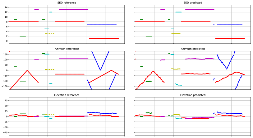
Figure 3: Visualization of SELD output for ACCDOA w/ RD3Net.

3.2 Experimental results

Table 2 shows the performance with the development set for our systems. As shown in the table, our systems outperformed the baseline for each metric by a large margin. We compared the performances of RD3Net and CRNN used in [1] with the ACCDOA system. The results show significant improvements over CRNN in all metrics, demonstrating the advantage of RD3Net. We also compared the performances of the ACCDOA system and two-stage system. The ACCDOA system showed 2.3 points higher ${LR}_{CD}$ than the two-stage in the testing split, while the ACCDOA system improved ${F}_{20^{\circ}}$ by 3.8 points. This suggests that the the ACCDOA system is more effective in the location-aware detection. Model ensemble improved ${F}_{20^{\circ}}$ by 3.2 points from the single model in the testing split. Table 3 shows the performances of the ACCDOA system ”Shimada_SONY_task3_1” on recordings without and with polyphony. We observed that the performance on recordings without polyphony is better than with polyphony.

An example of the proposed ACCDOA system output from the test split is visuarized in Fig. 3. Each event class is represented by a unique color. We can observe that our system performs joint detection, localization, and tracking of dynamic sources successfully in the recording.

4 Conclusion

We presented our approach to DCASE2020 task 3, Sound Event Localization and Detection. Our systems use the ACCDOA representation to solve both SED and SEL tasks in a unified manner. Moreover, we proposed an efficient network architecture called RD3Net. Our systems showed superior performance over the baselines with a single model. Furthermore, we observed further improvement with an ensemble of the ACCDOA and two-stage systems.

5 Acknowledgement

We would like to thank Yuichiro Koyama for the useful discussions on ACCDOA.

References

- [1] Y. Cao, Q. Kong, T. Iqbal, F. An, W. Wang, and M. D. Plumbley, “Polyphonic sound event detection and localization using a two-stage strategy,” arXiv preprint arXiv:1905.00268, 2019.
- [2] N. Takahashi, M. Gygli, B. Pfister, and L. V. Gool, “Deep convolutional neural networks and data augmentation for acoustic event detection,” in Proc. Interspeech, 2016.
- [3] N. Takahashi, M. Gygli, and L. Van Gool, “Aenet: Learning deep audio features for video analysis,” IEEE Trans. on Multimedia, vol. 20, pp. 513–524, 2017.
- [4] L. Mazzon, Y. Koizumi, M. Yasuda, and N. Harada, “First order ambisonics domain spatial augmentation for dnn-based direction of arrival estimation,” in Proc. of DCASE Workshop, 2019.
- [5] D. S. Park, W. Chan, Y. Zhang, C.-C. Chiu, B. Zoph, E. D. Cubuk, and Q. V. Le, “SpecAugment: A simple data augmentation method for automatic speech recognition,” Proc. of Interspeech, pp. 2613–2617, 2019.
- [6] J. Zhang, W. Ding, and L. He, “Data augmentation and prior knowledge-based regularization for sound event localization and detection,” in Tech. Report of DCASE Challenge, 2019.
- [7] N. Takahashi and Y. Mitsufuji, “D3Net: Densely connected multidilated DenseNet for music source separation,” arXiv preprint arXiv:2010.01733, 2020. [Online]. Available: https://arxiv.org/abs/2010.01733
- [8] C. Ye, M. Evanusa, H. He, A. Mitrokhin, T. Goldstein, J. A. Yorke, C. Fermuller, and Y. Aloimonos, “Network deconvolution,” in Proc. ICLR, 2020.
- [9] V. Lostanlen, J. Salamon, M. Cartwright, B. McFee, A. Farnsworth, S. Kelling, and J. P. Bello, “Per-channel energy normalization: Why and how,” IEEE Signal Processing Letters, vol. 26, no. 1, pp. 39–43, 2018.
- [10] Z.-Q. Wang, J. Le Roux, and J. R. Hershey, “Multi-channel deep clustering: Discriminative spectral and spatial embeddings for speaker-independent speech separation,” in Proc. of IEEE ICASSP, 2018, pp. 1–5.
- [11] A. Politis, S. Adavanne, and T. Virtanen, “A dataset of reverberant spatial sound scenes with moving sources for sound event localization and detection,” arXiv preprint arXiv:2006.01919, 2020.
- [12] A. Mesaros, S. Adavanne, A. Politis, T. Heittola, and T. Virtanen, “Joint measurement of localization and detection of sound events,” in Proc. of IEEE WASPAA, 2019.
- [13] H. Erdogan and T. Yoshioka, “Investigations on data augmentation and loss functions for deep learning based speech-background separation,” in Proc. of Interspeech, 2018, pp. 3499–3503.