A General Class of Transfer Learning Regression without Implementation Cost

Abstract

We propose a novel framework that unifies and extends existing methods of transfer learning (TL) for regression. To bridge a pretrained source model to the model on a target task, we introduce a density-ratio reweighting function, which is estimated through the Bayesian framework with a specific prior distribution. By changing two intrinsic hyperparameters and the choice of the density-ratio model, the proposed method can integrate three popular methods of TL: TL based on cross-domain similarity regularization, a probabilistic TL using the density-ratio estimation, and fine-tuning of pretrained neural networks. Moreover, the proposed method can benefit from its simple implementation without any additional cost; the regression model can be fully trained using off-the-shelf libraries for supervised learning in which the original output variable is simply transformed to a new output variable. We demonstrate its simplicity, generality, and applicability using various real data applications.

1 Introduction

Transfer learning (TL) (Pan and Yang 2009; Yang et al. 2020) is an increasingly popular machine learning framework that covers a broad range of techniques of repurposing a set of pretrained models on source tasks for another task of interest. It is proven that TL has the potential to improve the prediction performance on the target task significantly, in particular, given a limited supply of training data in which the learning from scratch is less effective. To date, the most outstanding successes of TL have been achieved by refining and reusing specific layers of deep neural networks (Yosinski et al. 2014). One or more layers in the pretrained neural networks are refined according to the new task using a limited target dataset. The remaining layers are either frozen (frozen featurizer) or almost unchanged (fine-tuning) during the cross-domain adaptation.

In this study, we aim to establish a new class of TL, which is applicable to any regression models. The proposed class unifies different classes of existing TL methods for regression. To model the transition from a pretrained model to a new model, we introduce a density-ratio reweighting function. The density-ratio function is estimated by conducting a Bayesian inference with a specific prior distribution while keeping the given source model unchanged. Two hyperparameters and the choice of the density-ratio model characterize the proposed class. It can integrate and extend three popular methods of TL within a unified framework, including TL based on the cross-domain similarity regularization (Jalem et al. 2018; Marx et al. 2005; Raina, Ng, and Koller 2006; Kuzborskij and Orabona 2013, 2017), probabilistic TL using the density-ratio estimation (Liu and Fukumizu 2016; Sugiyama, Suzuki, and Kanamori 2012), and the fine-tuning of pretrained neural networks (Hinton, Vinyals, and Dean 2015; Kirkpatrick et al. 2017; Yosinski et al. 2014).

In general, the model transfer operates through a regularization scheme to leverage the transferred knowledge between different tasks. A conventional regularization aims to retain similarity between the pretrained and transferred models. This natural idea is what we referred to as the cross-domain similarity regularization. On the other hand, the density-ratio method operates with an opposite learning objective that we call the cross-domain dissimilarity regularization; the discrepancy between two tasks is modeled and inferred, and the transferred model is a weighted sum of the pretrained source model and the newly trained model on the discrepancy. These totally different methods can be unified within the proposed framework.

To summarize, the features and contributions of our method are as follows:

• The method can operate with any kinds of regression models.

• The proposed class, which has two hyperparameters, can unify and hybridize three existing methods of TL, including the regularization based on cross-domain similarity and dissimilarity.

• The two hyperparameters and a model for the density-ratio function are selected through cross-validation. With this unified workflow, an ordinary supervised learning without transfer can also be chosen if the previous learning experience interferes with learning in the new task.

• The proposed method can be implemented with no extra cost. With a simple transformation of the output variable, the model can be trained using off-the-shelf libraries for regression that implement the $\ell_{2}$-loss minimization with any regularization scheme. In addition, the method is applicable in scenarios where only the source model is accessible but not the source data, for example, due to privacy reasons.

Practical benefits of bridging totally different methods in the unified workflow are tested on a wide range of prediction tasks in science and engineering applications.

2 Proposed method

We are given a pretrained model $y=f_{s}(x)$ on the source task, which defines the mapping between any input $x$ to a real-valued output $y\in\mathbb{R}$. The objective is to transform the given $f_{s}(x)$ into a target model $y=f_{t}(x)$ by using $n$ instances from the target domain, $\mathcal{D}=\{(x_{i},y_{i})\}_{i=1}^{n}$.

Inspired by (Liu and Fukumizu 2016), we apply the probabilistic modeling for the transition from $f_{s}(x)$ to $f_{t}(x)$. With the conditional distribution $p_{s}(y|x)$ of the source task, the one on the target can be written as

$$p_{t}(y|x)=w(y,x)p_{s}(y|x)$$

where $w(y,x)=p_{t}(y|x)/p_{s}(y|x)$. Consider that the source distribution is modelled by $p_{s}(y|x,f_{s})$ which involves the pretrained $f_{s}(x)$. In addition, the density-ratio function $w(y,x)$ is separately modeled as $w(y,x|\theta_{w})$ with an unknown parameter $\theta_{w}$, which will be associated with a regression model $f_{\theta_{w}}(x)$. The target model $p_{t}(y|x,\theta_{w})$ is then

$$p_{t}(y|x,\theta_{w})\!\!\!\! = \!\!\!\!w(y,x|\theta_{w})p_{s}(y|x,f_{s})$$ (1)

such that $$\forall \!\!\!\!\!\!x:\int w(y,x|\theta_{w})p_{s}(y|x,f_{s})\mathrm{d}y=1,$$

where the normalization constraint is due to the fact that the conditional probability needs to be normalized to 1 over its domain.

We employ Bayesian inference to estimate the unknown $\theta_{w}$ in the density-ratio model $w(y,x|\theta_{w})$. The target model $p_{t}(y|x,\theta_{w})$ is used as the likelihood for Bayesian inference, and a prior distribution $p(\theta_{w}|f_{s})$ is placed on $\theta_{w}$, which depends on the given $f_{s}$. The posterior distribution is then

$$p(\theta_{w}|\mathcal{D})\propto\prod_{i=1}^{n}p_{t}(y_{i}|x_{i},\theta_{w})p(\theta_{w}|f_{s}).$$ (2)

We adopt Gaussian models for the likelihood function as

$$w(y,x|\theta_{w})\!\!\!\! \propto \!\!\!\!{\rm exp}\left(-\frac{(y-f_{\theta_{w}}(x))^{2}}{\sigma}\right),$$ (3)

$$p_{s}(y|x,f_{s})\!\!\!\! \propto \!\!\!\!{\rm exp}\left(-\frac{(y-f_{s}(x))^{2}}{\eta}\right),$$ (4)

where $\sigma>0$ and $\eta>0$. The normalization constant for the product of the two expressions on the right-hand side of Eq. 3 and Eq. 4 is given as ${\rm exp}\left(-(\sigma+\eta)^{-1}(f_{s}(x)-f_{\theta_{w}}(x))^{2}\right)$, which depends on the proximity of $f_{\theta_{w}}(x)$ to $f_{s}(x)$. In addition, we regularize the training based on the discrepancy of the two models $f_{\theta_{w}}(x)$ and $f_{s}(x)$, which can belong to different classes of regression models. In order to do so, we introduce a prior distribution that implements a function-based regularization as

$$p(\theta_{w}|f_{s})\propto{\rm exp}\left(-\sum_{i=1}^{m}\frac{(f_{s}(u_{i})-f_{\theta_{w}}(u_{i}))^{2}}{\lambda}\right),$$ (5)

where $\lambda\in\mathbb{R}\backslash\{0\}$. The discrepancy is measured by the sum of their squared distances over $m$ input values $\mathcal{U}=\{u_{i}\}_{i=1}^{m}$. Hereafter, we use the $n$ observed inputs in $\mathcal{D}$ for $\mathcal{U}$. The posterior distribution involves three hyperparameters $(\sigma,\eta,\lambda)$. Note that $\lambda$ can be either positive or negative and controls the degree of discrepancy, positively or negatively. As described below, this Gaussian-type modeling leads to an analytic workflow that can benefit from less effort on the implementation.

We consider the Maximum a Posteriori (MAP) estimation of $\theta_{w}$ and a class of prediction functions $\hat{y}(x)$ that are characterized by two hyperparameters $\tau$ and $\rho$:

$$\hat{\theta}_{w} \!\!\!\!\!\!\!\!=\mathop{\rm arg~{}min}\limits_{\theta_{w}}\!\displaystyle\sum_{i=1}^{n}\!\big{\{}\!(y_{i}\!-\!f_{\theta_{w}}(x_{i}))^{2}\!-\!\tau(f_{s}(x_{i})\!-\!f_{\theta_{w}}(x_{i}))^{2}\!\big{\}},$$

$$\hat{y}(x) \!\!\!\!\!\!=\!\mathrm{argmax}_{y}\ p_{t}(y|x,\hat{\theta}_{w})\!=\!(1-\rho)f_{\hat{\theta}_{w}}(x)+\rho f_{s}(x),$$

$$\tau \!\!\!\!\!\!\!\!=\frac{\sigma}{\sigma+\eta}-\frac{\sigma}{\lambda}\in(-\infty,1),\ \ \rho=\frac{\sigma}{\sigma+\eta}\in(0,1).$$

In the training objective Eq. 2, the first term measures the goodness-of-fit with respect to $\mathcal{D}$. The second term is derived from the normalization term in Eq. 1 and the prior distribution Eq. 5. It regularizes the training through the discrepancy between $f_{\theta_{w}}(x)$ and the pretrained $f_{s}(x)$. The prediction function Eq. 2 corresponds to the mode of the plug-in predictive distribution Eq. 1. Note that the original three hyperparameters are reduced to $\tau\in(-\infty,1)$ and $\rho\in(0,1)$. By varying $(\tau,\rho)$ and different models on $f_{\theta_{w}}(x)$ coupled with the learning algorithms, the resulting method can bridge various methods of TL as described later.

3 Implementation cost

By completing the square of Eq. 2 with respect to $f_{\theta_{w}}(x)$, the objective function can be rewritten as a residual sum of squares on a transformed output variable $z$:

$$\hat{\theta}_{w}\!=\!\mathop{\rm arg~{}min}\limits_{\theta_{w}}\!\displaystyle\sum_{i=1}^{n}(z_{i}\!-\!f_{\theta_{w}}(x_{i}))^{2},\hskip 7.0ptz_{i}=\frac{y_{i}\!-\!\tau f_{s}(x_{i})}{1-\tau}.$$

Once the original output $y_{i}$ is simply converted to $z_{i}$ with a given $f_{s}(x)$ and $\tau$, the model can be trained by using a common $\ell_{2}$-loss minimization library for regression. Any regularization term, such as $\ell_{1}$- or $\ell_{2}$-regularization, can also be added. Therefore, the proposed method can be implemented at essentially no cost. In the applications shown later, we utilized ridge regression, random forest regression, and neural networks as $f_{\theta_{w}}(x)$. We simply used the standard libraries of the R language (glmnet, ranger, and MXNet) without any customization or additional coding.

Furthermore, as no source data appear in the objective function, the model is learnable by using only training instances in a target domain as long as a source model is callable. This separately learnable property will be a great advantage in cases, for example, where training the source model from scratch is time-consuming, or the source data can not be disclosed.

4 Relations to existing methods

By adjusting $(\tau,\rho)$ coupled with the choice of $f_{\theta_{w}}(x)$, our method can represent the different types of TL as described below. The relationship between different methods are visually overviewed in Figure 1.

Regularization based on cross-domain similarity

One of the most natural ideas for model refinement is to use the similarity to the pretrained $f_{s}(x)$ as a constraint condition. Many studies have been made so far to incorporate such cross-domain similarity regularization to TL or other related machine learning tasks such as avoiding catastrophic forgetting in continual lifelong learning (Kirkpatrick et al. 2017), knowledge distillation to compress pretrained complex neural networks efficiently to simpler models (Hinton, Vinyals, and Dean 2015).

Here, this type of regularization is described in a Bayesian fashion. We consider a posterior distribution in Eq. 2, but impose the Gaussian distribution on the likelihood $p_{t}(y|x,\theta_{w})=\mathcal{N}(y|f_{\theta_{w}}(x),\sigma)$ and the same prior to Eq. 5 is imposed to $p(\theta_{w}|f_{s})$. Then, the MAP estimator for $\theta_{w}$ and the mode of the plug-in predictive distribution are of the following form

$$\hat{\theta}_{w} \!\!\!\!\!\!\!\!=\mathop{\rm arg~{}min}\limits_{\theta_{w}}\!\sum_{i=1}^{n}\!\big{\{}\!(y_{i}\!-\!f_{\theta_{w}}(x_{i}))^{2}+\cfrac{\sigma}{\lambda}(f_{s}(x_{i})\!-\!f_{\theta_{w}}(x_{i}))^{2}\!\big{\}},$$ (9)

$$\hat{y}(x) \!\!\!\!\!=f_{\hat{\theta}_{w}}(x).$$

The objective function of our method Eq. 2 can represent the MAP estimation with the objective function in Eq. 9 by restricting the hyperparameter $\tau$ (or $\lambda$) to be negative, i.e., $\tau=-\sigma/\lambda<0$. The prediction function in Eq. 9 corresponds to $\rho=0$ in our method. With a negative $\tau$, the model $f_{\theta_{w}}(x)$ is estimated to be closer to the pretrained source model. Such a newly trained model $f_{\hat{\theta}_{w}}(x)$ is directly used as the prediction function without using the source model.

Transfer learning based on neural networks

To our best knowledge, the most powerful and widely used method of TL relies on deep neural networks (Yosinski et al. 2014). When neural networks are put on both $f_{\theta_{w}}(x)$ and $f_{s}(x)$ in the objective function Eq. 9, the pretrained $f_{s}(x)$ is fine-tuned to $f_{\theta_{w}}(x)$ by retaining the cross-domain similarity between their output layers.

Figure 1: Existing methods mapped onto the hyperparameter space $(\tau,\rho)$. The cross-domain similarity regularization corresponds to $\tau<0$ and $\rho=0$ (black line). If neural networks are put on both $f_{\theta_{w}}(x)$ and $f_{s}(x)$, this region corresponds to the fine-tuning of neural networks. If $\tau=\rho$ (blue line), the class represents the density-ratio TL. The region with $\tau=\rho=0$ (black dot) or $\rho=1$ (red line) represents an ordinal regression without transfer or the case where a source model is directly used as the target, respectively.

Transfer learning based on the density-ratio estimation

The density-ratio TL of (Liu and Fukumizu 2016) was designed to minimize the conditional Kullback-Leibler divergence $\mathbb{E}_{x\sim q(x)}[{\rm KL}(q(y|x)||p_{t}(y|x,\theta_{w}))]$ between the true density $q(y|x)$ and the transferred model $p_{t}(y|x,\theta_{w})$ based on the density-ratio reweighting as in Eq. 1. As detailed in Supplementary Note A, if the transfer model is paramterized in the same way as Eq. 3, the learning objective derived from an empirical risk on the training set $\mathcal{D}$ takes the form

$$\hat{\theta}_{w} \!\!\!\!\!\!=\mathop{\rm arg~{}min}\limits_{\theta_{w}}\!\sum_{i=1}^{n}\Big{\{}\!(y_{i}\!-\!f_{\theta_{w}}(x_{i}))^{2}-\rho(f_{s}(x_{i})\!-\!f_{\theta_{w}}(x_{i}))^{2}\!\Big{\}},$$

$$\rho \!\!\!\!\!\!=\frac{\sigma}{\sigma+\eta}\in(0,1).$$

The second term represents the discrepancy between the density-ratio model and the source model in which the degree of regularizaion is controlled by $\rho\in(0,1)$. For the prediction function, as with Eq. 2, we consider $\hat{y}(x)=(1-\rho)f_{\hat{\theta}_{w}}(x)+\rho f_{s}(x)$ that corresponds to the plug-in estimator $\mathrm{argmax}_{y}\ p_{t}(y|x,\hat{\theta}_{w})$.

In terms of the proposed class of TL, the method in (Liu and Fukumizu 2016) can be considered as a specific choice of $\tau=\rho\in(0,1)$ (the blue line in Figure 1). This corresponds to the case where $\lambda$ in Eq. 5 is sufficiently large, i.e., the prior distribution for the parameters of the density-ratio function is uniformly distributed and non-informative. It is noted that the objective function in Eq. 4 resembles Eq. 9 in the cross-domain similarity regularization. These two methods are regularized based on the discrepancy between $f_{\theta_{w}}(x)$ and $f_{s}(x)$, but their regularization mechanisms work in the opposite directions: the regularization parameter $\tau$ takes a positive value for the method in (Liu and Fukumizu 2016), which we call cross-domain dissimilarity regularization, while a negative value for cross-domain similarity regularization.

Learning without transfer

The proposed family of methods contains two learning schemes without transfer. If the hyperparameters are selected to be $\tau=0$ and $\rho=0$ (the black dot in Figure 1), the density-ratio model $\hat{f}_{\theta_{w}}(x)$ is estimated without using the source model, and the resulting prediction model becomes $\hat{y}(x)=f_{\hat{\theta}_{w}}(x)$. This corresponds to an ordinary regression procedure. When negative transfer occurs i.e., the previous learning experience interferes with learning in the new task, the desirable hyperparameters would be around $\tau=0$ and $\rho=0$ . In addition, setting $\rho=1$ (the red line in Figure 1), the source model alone gives the prediction model as $\hat{y}(x)=f_{s}(x)$ regardless of $f_{\theta_{w}}(s)$. By cross-validating the hyperparameters, the proposed framework will automatically determine when not to transfer without using a separate pipelines.

5 Selection of hyperparameters and preference to bias and variance

As described above, our method can hybridize various mechanisms of TL by adjusting $\tau$ and $\rho$. The values of the hyperparameters are adjusted through cross-validation. Clearly, the optimal combination of the hyperparameters will differ depending on between-task relationships and the choice for the target model.

Here, we show an expression of the mean squared error (MSE) based on the bias-variance decomposition. For simplicity, we restrict $f_{\hat{\theta}_{w}}(x)$ to be in the set of all linear predictions taking the form of $f_{\hat{\theta}_{w}}(x)=x^{\mathsf{T}}{\rm S}{\bf z}$. The $n\times n$ smoothing matrix $\rm S$ depends on $n$ samples of $p$ input feature $\mathbf{\phi}(x_{i})\in\mathbb{R}^{p}$ ($i=1,\ldots,n$) with a predefined basis set $\mathbf{\phi}$, and $\bf z$ is a vector of $n$ transformed outputs $z_{i}$ ($i=1,\ldots,n$). For example, this class of prediction includes the kernel ridge regression.

We assume that $y$ follows $y=f_{t}(x)+\epsilon$ where $f_{t}(x)$ denotes the true model and the observation noise $\epsilon$ has mean zero and variance $\sigma_{\epsilon}^{2}$. For the prediction function $\hat{y}(x)=(1-\rho)f_{\hat{\theta}_{w}}(x)+\rho f_{s}(x)$, ${\rm MSE}(\hat{y}(x))=\mathbb{E}_{y|x}[y-\hat{y}(x)]^{2}$ can be expressed as:

$${\rm MSE}(\hat{y}(x))\!\!\!\!\!\! = \!\!\!\!\!\left[\frac{\rho\!-\!\tau}{1\!-\!\tau}{\rm D}(x)+\frac{1\!-\!\rho}{1\!-\!\tau}{\rm B}_{1}(x)-\frac{\tau(1\!-\!\rho)}{1\!-\!\tau}{\rm B}_{2}(x)\right]^{2}$$ (11)

$$+ \!\!\!\!\left(\frac{1\!-\!\rho}{1\!-\!\tau}\right)^{2}{\rm V}(x)+\sigma_{\epsilon}^{2},$$

where

$${\rm D}(x)\!\!\!\! = \!\!\!\!f_{t}(x)-f_{s}(x),$$

$${\rm B}_{1}(x)\!\!\!\! = \!\!\!\!f_{t}(x)-x^{\mathsf{T}}{\rm S}{\bf f}_{t},$$

$${\rm B}_{2}(x)\!\!\!\! = \!\!\!\!f_{s}(x)-x^{\mathsf{T}}{\rm S}{\bf f}_{s},$$

$${\rm V}(x)\!\!\!\! = \!\!\!\!\sigma_{\epsilon}^{2}x^{\mathsf{T}}{\rm S}{\rm S}^{\mathsf{T}}x.$$

The first term is the squared bias, which consists of three building blocks. ${\rm D}(x)$ represents the discrepancy between $f_{t}(x)$ and $f_{s}(x)$. ${\rm B}_{1}(x)$ is a bias of the linear estimator $x^{\mathsf{T}}{\rm S}{\bf f_{t}}$ with respect to the true model $f_{t}(x)$, assuming that $n$ observations ${\bf f}_{t}=(f_{t}(x_{1}),\ldots,f_{t}(x_{n}))^{\mathsf{T}}$ for the unknown $f_{t}(x)$ are given. Likewise, ${\rm B}_{2}(x)$ is the bias of $x^{\mathsf{T}}{\rm S}{\bf f_{s}}$ with respect to $f_{s}(x)$. The second term corresponds to the variance of $\hat{y}(x)$. This is proportional to ${\rm V}(x)=\sigma_{\epsilon}^{2}x^{\mathsf{T}}{\rm S}{\rm S}^{\mathsf{T}}x$. The third term is the variance of the observation noise.

The relative magnitudes of $\mathbb{E}_{x}[{\rm D}(x)^{2}]$, $\mathbb{E}_{x}[{\rm B}_{1}(x)^{2}]$, $\mathbb{E}_{x}[{\rm B}_{2}(x)^{2}]$, and $\mathbb{E}_{x}[{\rm V}(x)]$ determine the optimal hyperparameters to the cross-domain similarity regularization, the density-ratio TL, and the learning without transfer. Let ${\rm D}={\rm D}(x)$, ${\rm B}_{1}={\rm B}_{1}(x)$, ${\rm B}_{2}={\rm B}_{2}(x)$, and ${\rm V}={\rm V}(x)$, respectively. Consider the expectation of the MSE in Eq. 11 with respect the marginal distribution of $x$: $\mathbb{E}_{x\sim q(x)}[{\rm MSE}(\hat{y}(x))]$. Because the expected MSE is quadratic with respect to $\rho$ for any $\tau$, the minimum under the inequality constraint $0\leq\rho\leq 1$ is achieved by

$$\rho(\tau)=\left\{\begin{array}[]{ll}0&\rho_{*}(\tau)\leq 0\\ \rho_{*}(\tau)&0<\rho_{*}(\tau)<1\\ 1&\rho_{*}(\tau)\geq 1\end{array}\right.$$ (15)

where $\rho_{*}(\tau)$ denotes the solution for the unconstrained minimization. Taking the derivative of the expected MSE with respect to $\rho$, we have an equation as

$$\frac{1}{(1-\tau)^{2}}\mathbb{E}[((\rho\!-\!\tau){\rm D}\!+\!(1\!-\!\rho){\rm B}_{1}-\!\!\!\!\!\!\! \tau \!\!\!\!\!\!\!(1\!-\!\rho){\rm B}_{2}))({\rm D}\!-\!{\rm B}_{1}\!+\!\tau{\rm B}_{2})]$$ (16)

$$- \!\!\!\!\!\!\frac{1-\rho}{(1-\tau)^{2}}\mathbb{E}[{\rm V}]=0.$$

Assuming that $\tau\neq 1$, this leads to an expression for the unconstrained solution as

$$\rho_{*}(\tau)=\frac{\mathbb{E}[(\tau{\rm D}-{\rm B}_{1}+\tau{\rm B}_{2})({\rm D}-{\rm B}_{1}+\tau{\rm B}_{2})]+\mathbb{E}[{\rm V}]}{\mathbb{E}[{\rm D}-{\rm B}_{1}+\tau{\rm B}_{2}]^{2}+\mathbb{E}[{\rm V}]}.$$ (17)

Likewise, taking the derivative of the expected MSE with respect to $\tau$, we have

$$\frac{1-\rho}{(1-\tau)^{3}}\mathbb{E}[((\rho\!-\!\tau){\rm D}\!+\!(1\!-\!\rho){\rm B}_{1}-\!\!\!\!\!\! \tau \!\!\!\!\!\!(1\!-\!\rho){\rm B}_{2}))({\rm D}\!-\!{\rm B}_{1}\!+\!{\rm B}_{2})]$$ (18)

$$- \!\!\!\!\!\!\frac{(1-\rho)^{2}}{(1-\tau)^{2}}\mathbb{E}[{\rm V}]=0.$$

Combining Eq. 16 and Eq. 18 where $\tau\neq 1$ and $\rho\neq 1$, we obtain an equation

$$(1-\tau)\mathbb{E}[\tau({\rm D}+(1-\rho){\rm B}_{2}){\rm B}_{2}-(1-\rho){\rm B}_{1}\!\!\!\!\!\! {\rm B}_{2} \!\!\!\!\!+\rho{\rm D}{\rm B}_{2}]$$

$$= \!\!\!\!\!\!0,$$

then yielding an expression for the solution

$$\tau(\rho)=\frac{(1-\rho)\mathbb{E}[{\rm B}_{1}{\rm B}_{2}]+\rho\mathbb{E}[{\rm D}{\rm B}_{2}]}{(1-\rho)\mathbb{E}[{\rm B}_{2}^{2}]+\mathbb{E}[{\rm D}{\rm B}_{2}]}.$$ (19)

According to the two expressions in Eq. 17 and Eq. 19, we can investigate the preference in the hyperparameter selection in regard to the bias and variance components in the data generation process.

Consider a case where the source and target models are significantly different by taking the limit $\mathbb{E}[{\rm D}^{2}]\rightarrow\infty$. For the expectation of $\mathbb{E}[{\rm D}{\rm X}]$ for the product of ${\rm D}$ and any ${\rm X}$, it holds that $\mathbb{E}[{\rm D}{\rm X}]/\mathbb{E}[{\rm D}^{2}]\rightarrow 0$ as $\mathbb{E}[{\rm D}^{2}]\rightarrow\infty$. This can be seen by considering the Cauchy-Schwarz inequality:

$$-\mathbb{E}[{\rm{D}^{2}}]^{\frac{1}{2}}\mathbb{E}[{\rm{X}^{2}}]^{\frac{1}{2}}\!\!\!\! \leq \!\!\!\!\mathbb{E}[{\rm{DX}}]\leq\mathbb{E}[{\rm{D}^{2}}]^{\frac{1}{2}}\mathbb{E}[{\rm{X}^{2}}]^{\frac{1}{2}}$$

$$\Leftrightarrow-\frac{\mathbb{E}[{\rm{X}^{2}}]^{\frac{1}{2}}}{\mathbb{E}[{\rm{D}^{2}}]^{\frac{1}{2}}}\!\!\!\! \leq \!\!\!\!\frac{\mathbb{E}[{\rm DX}]}{\mathbb{E}[{\rm D}^{2}]}\leq\frac{\mathbb{E}[{\rm X}^{2}]^{\frac{1}{2}}}{\mathbb{E}[{\rm{D}^{2}}]^{\frac{1}{2}}}.$$

In the second line, the upper- and the lower-bounds go to zero as $\mathbb{E}[{\rm D}^{2}]\rightarrow\infty$. Thus, in Eq. 17, all terms except those having $\mathbb{E}[{\rm D}^{2}]$, which appear in its numerator and denominator, approach asymptotically to zero, which results in

$$\rho_{*}(\tau)\rightarrow\frac{\tau\mathbb{E}[{\rm D}^{2}]}{\mathbb{E}[{\rm D}^{2}]}=\tau\ \ \mathrm{as}\ \ \mathbb{E}[{\rm D}^{2}]\rightarrow\infty.$$

Furthermore, noting that $\mathbb{E}[{\rm DX}]=O(\mathbb{E}[{\rm D}^{2}]^{\frac{1}{2}})$, it can been seen that $\tau(\rho)$ in Eq. 19 approaches asymptotically $\rho$:

$$\tau(\rho)\rightarrow\frac{\rho\mathbb{E}[{\rm DB}_{2}]}{\mathbb{E}[{\rm DB}_{2}]}=\rho\ \ \mathrm{as}\ \ \mathbb{E}[{\rm D}^{2}]\rightarrow\infty.$$

Therefore, when ${\mathbb{E}[{\rm D}^{2}]}$ dominates the other three quantities, the density-ratio TL ($\tau=\rho$) is preferred. This fact accounts for the experimental observations presented above.

Figure 2: Heatmap display of the MSE landscape on the hyperparameter space ($\tau$, $\rho$) that changes as a function of the bias ($\alpha$) and variance ($\sigma_{\epsilon}$). With given $\tau$ and $\rho$, the linear ridge regression was used to train $f_{\theta_{w}}(x)$ on the artificial data. The black dot denotes the lowest MSE.

On the other hand, if the source and target models are completely the same (${\mathbb{E}[{\rm D}^{2}]}=0$), it holds that $\rho_{*}(\tau)=1$. Alternatively, if ${\mathbb{E}[{\rm V}]}\rightarrow\infty$, $\rho_{*}(\tau)=1$. The direct use of the source model as a prediction function tends to be optimal as the source and target tasks get closer or the variance ${\mathbb{E}[{\rm V}]}$ becomes larger. It has not yet been clear when the cross-domain similarity regularization would be preferred, either theoretically or experimentally.

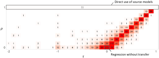
Figure 3: Distribution of $(\tau,\rho)$ that delivered the lowest MSE in 1,665 cases (185 task pairs and $3^{2}$ combinations of models for $f_{s}(x)$ and $f_{\theta_{w}}(x)$). The number in each pixel denotes the count of cases.

Table 1: Selected hyperparameters (the last three columns, representing hyperparameters $\tau$ and $\rho$) and their corresponding MSEs (the 4-6th columns) for the TL from one source task to five target tasks. Three different models (LN: linear, RF: random forests, and NN: neural networks) were applied to $f_{s}(x)$ and $f_{\theta_{w}}(x)$. Supplementary Note C provides full results for all the 1,665 cases.

Source task	Target task	$f_{s}(x)$	$f_{\theta_{w}}(x)$			Selected hyperparameters
			LN	RF	NN	LN	RF	NN
Monomer -  Dielectric constant	Monomer -  HOMO-LUMO gap	LN	0.8292	0.7435	0.8823	(-0.1, 0.1)	( 0.6, 0.4)	( 0.1, 0.3)
		RF	0.8302	0.7139	0.7421	(-0.1, 0.2)	( 0.5, 0.3)	( 0.8, 0.8)
		NN	0.8250	0.7372	0.7644	(-0.2, 0.2)	( 0.2, 0.3)	( 0.4, 0.4)
	Monomer -  Refractive index	LN	0.0436	0.0424	0.0439	( 0.8, 0.9)	( 0.8, 0.9)	( 0.8, 0.9)
		RF	0.0463	0.0415	0.0415	( 0.9, 0.9)	(  -  , 1.0)	(  -  , 1.0)
		NN	0.0365	0.0355	0.0505	( 0.8, 0.9)	( 0.8, 0.9)	( 0.4, 0.7)
	Polymer -  Band gap	LN	1.0881	0.7862	0.8936	( 0.3, 0.1)	( 0.0, 0.1)	( 0.6, 0.6)
		RF	0.8594	0.7477	0.7130	(-0.2, 0.4)	( 0.4, 0.3)	( 0.8, 0.8)
		NN	0.8654	0.8598	0.8908	(-0.5, 0.1)	( 0.3, 0.5)	( 0.6, 0.5)
	Polymer -  Dielectric constant	LN	0.6031	0.5358	0.6376	(-0.4, 0.2)	( 0.3, 0.2)	(-0.5, 0.0)
		RF	0.5988	0.5786	0.6678	(-0.2, 0.2)	( 0.3, 0.2)	( 0.0, 0.4)
		NN	0.6143	0.5478	0.7563	(-0.1, 0.2)	( 0.2, 0.3)	(-0.2, 0.1)
	Polymer -  Refractive index	LN	0.3269	0.3906	0.3442	( 0.0, 0.0)	(-0.4, 0.0)	( 0.2, 0.4)
		RF	0.3269	0.3574	0.3312	( 0.0, 0.0)	( 0.1, 0.1)	( 0.1, 0.2)
		NN	0.3269	0.3845	0.4254	( 0.0, 0.0)	(-0.1, 0.1)	(-1.7, 0.0)

6 Results

Illustrative example

Some intrinsic properties of the proposed method are illustrated by presenting numerical examples using artificial data. According to our experience, there is a link between the bias and variance magnitudes and the hyperparameters that minimize the MSE. This will be demonstrated.

We assumed the true functions on the source and target tasks to be linear as $f_{t}(x)=x^{\mathsf{T}}\theta_{t}$ and $f_{s}(x)=x^{\mathsf{T}}\theta_{s}$ where $x\in\mathbb{R}^{300}$. The true parameters were generated as $\theta_{t}=\alpha\theta_{s}+(1-\alpha)\theta_{w}$ where $\theta_{s}\sim\mathcal{N}(0,{\rm I})$ and $\theta_{w}\sim\mathcal{N}(0,{\rm I})$. The output variable was assumed to follow $y=f_{t}(x)+\epsilon$ where $x\sim\mathcal{N}(0,{\rm I})$ and $\epsilon\sim\mathcal{N}(0,{\rm\sigma_{\epsilon}^{2}})$. With the given $\theta_{w}$ and $\theta_{s}$, we generated $\{x_{i},y_{i}\}_{i=1}^{n}$ with the sample size set to $n=50$ by randomly sampling $x$ and $\epsilon$. The discrepancy between the source and target models is controlled by the mixing rate $\alpha\in[0,1]$ for any given $\theta_{w}$. In particular, if $\alpha$ is set to zero, the source and target models are the same ($\forall x$: ${\rm D}(x)=0$ in Eq. 11). The variance $\sigma_{\epsilon}^{2}$ of the observational noises affects the magnitude of the variance $\mathbb{E}[\rm{V}]$ in the model estimation.

We used the linear ridge regression to estimate $f_{\theta_{w}}$ with the hyperparameter on the $\ell_{2}$-regularization that was fixed at $\lambda=0.0001$. The true source model was used as $f_{s}(z)$. We then investigated the change of the MSE landscape as a function of the bias $\alpha$ and the variance $\sigma_{\epsilon}$, which are summarized in Figure 2. For any given values of $\tau$ and $\rho$, the MSE was approximately evaluated by averaging the $\ell_{2}$-loss over additionally generated 1,000 samples on $(x,y)$ and rescaled to the range in $[0,1]$. For $\alpha=0$ where the source and target models are the same, the MSE became small in the region along $\rho=1$ that corresponds to the use of the pretrained source model as the target model with no modification. As $\alpha$ increased while keeping $\sigma_{\epsilon}$ at smaller values, the region where the MSE becomes small was concentrated around $\tau=\rho$, indicating the dominant performance of the density-ratio TL. On the other hand, as both $\alpha$ and $\sigma_{\epsilon}$ became larger, the region with $\tau<0$ and $\rho=0$ tended to be more favored. This region corresponds to the TL with the cross-domain similarity regularization. It was confirmed that the pattern of the MSE landscape varies continuously with respect to the bias and variance components.

In many other applications, we have often observed the same trend on the preference of $\tau$ and $\rho$ with respect to the relative magnitude of the bias and variance. Another example assuming nonlinear models for $f_{s}(x)$ and $f_{t}(x)$, and random forests for $f_{\theta_{w}}(x)$ is shown in Supplementary Note B.

Real data applications

Task, data and analysis procedure

The proposed method was applied to five real data analyses in materials science and robotics applications: (i) multiple properties of organic polymers and inorganic compounds (Yamada et al. 2019), (ii) multiple properties of polymers (Kim et al. 2018) and low-molecular-weight compounds (monomers, unpublished data), (iii) properties of donor molecules in organic solar cells (Paul et al. 2019) obtained from experiments (Lopez et al. 2016) and quantum chemical calculations (Pyzer-Knapp, Li, and Aspuru-Guzik 2015), (iv) formation energies of various inorganic compounds and crystal polymorphisms of SiO₂ and CdI₂ (Jain et al. 2013), and (v) the feed-forward torques required to follow a desired trajectory at seven joints of a SARCOS anthropomorphic robot arm (Williams and Rasmussen 2006). The model transfers were conducted exhaustively between all task pairs within each application, which resulted in a total of 185 pairs of the source and target tasks with 9 different combinations of $f_{s}(x)$ and $f_{\theta_{w}}(x)$ (a total of 1,665 cases).

For each task pair, we used three machine learning algorithms; Ridge regression using a linear model (LN), random forests (RF), and neural networks (NN) to estimate $f_{s}(x)$ and $f_{\theta_{w}}(x)$. In the source task, the entire dataset was used to train $f_{s}(x)$ under default settings of software packages without adjusting hyperparameters. In all cases, 50 randomly selected samples were used to train $f_{\theta_{w}}(x)$. We choose the best model based on the 5-fold cross validation. The resulting model was used to predict all the remaining data, and the MSE was evaluated. Details of the datasets and analysis procedure are presented in Supplementary Note C.

Figure 4: The MSE landscapes of the hyperparameter space for four different cases that exhibited the best transferability in different hyperparameter sets. Sample estimates on three bias-related quantities ($\mathbb{E}_{x}[{\rm D}^{2}]$, $\mathbb{E}_{x}[{{\rm B}_{1}}^{2}]$, and $\mathbb{E}_{x}[{{\rm B}_{2}}^{2}]$) and the mean variance ($\mathbb{E}_{x}[{\rm V}]$) are shown on each plot.

Results

Throughout all the 1,665 cases, we investigated how the hyperparameters selected by the cross-validation are distributed (Figure 3). In many cases, the distribution of the selected hyperparameters was concentrated in the neighboring areas of the density-ratio TL ($\tau=\rho$) and the cross-domain similarity regularization ($\tau<0,\rho=0$). The density-ratio TL was selected for 609 cases (36.6%) and the cross-domain similarity regularization was selected for 176 cases (10.6%). In particular, there was a significant bias toward the neighbors of $\tau=\rho$.

The selected hyperparameters and the MSEs for the 1,665 cases are presented in Tables S1-S5 of the Supplementary Note. As an illustrative example, Table 1 shows the result of the TL from one source task (prediction of a dielectric property of small molecules) to five target tasks (prediction of two properties of small molecules and three properties of polymers). This result also indicates the presence of bias toward $\tau$ and $\rho$. It was also observed that in some cases the choice of the density-ratio model significantly affects the prediction performance and in other cases it does not.

We speculate that the four quantities $\mathbb{E}_{x}[{\rm D}^{2}]$, $\mathbb{E}_{x}[{\rm B}_{1}^{2}]$, $\mathbb{E}_{x}[{\rm B}_{2}^{2}]$ and $\mathbb{E}_{x}[{\rm V}]$ or their counterparts in general regression, determine the preference of $\tau$ and $\rho$. Figure 4 shows the MSE mapped on the hyperparameter space and the four quantities for four task pairs. They were selected as the typical cases where the four different learning schemes are preferred. The proposed method exhibited the preference to direct use of source models when the difference between the source and target domains ($\mathbb{E}_{x}[{\rm D}^{2}]$) was small. When $\mathbb{E}_{x}[{\rm D}^{2}]$ was large, the relative magnitude of $\mathbb{E}_{x}[{\rm D}^{2}]$ and the other three quantities $\mathbb{E}_{x}[{{\rm B}_{1}}^{2}]$, $\mathbb{E}_{x}[{{\rm B}_{2}}^{2}]$ and $\mathbb{E}_{x}[{\rm V}]$ would determine the choice; if $\mathbb{E}_{x}[{\rm V}]$ was small, the density-ratio TL was preferred, and if $\mathbb{E}_{x}[{\rm V}]$ was large, the cross-domain similarity regularization was preferred. Furthermore, when both $\mathbb{E}_{x}[{{\rm B}_{1}}^{2}]$ and $\mathbb{E}_{x}[{\rm V}]$ were small, training without transfer was preferred. Such relationships were often observed in other cases as well. However, these are only views derived from partial observations, and there would be more complex factors to work in the learning mechanism. Supplementary Note C shows the results of investigating the magnitudes of the bias and variance and the selected hyperparameters for all cases.

7 Concluding remarks

We proposed a new class of TL that is characterized by two hyperparameters which in turn control training and prediction procedure. This new class of TL unifies two different types of existing methods that are based on the cross-domain similarity regularization and the density-ratio estimation. If we use neural networks on the source and target models, the class represents the fine tuning of neural networks. In addition, some specific selection of hyperparameters offers the choice of ordinary regression without transfer or the direct use of a pretrained source model as the target. According to the choice of hyperparameters and models, we can derive various learning methods in which these two methods are hybridized.

The cross-domain similarity regularization and the density-ratio TL follow opposite learning objectives. In the former case, the target model is regularized as being closer to the source model. In the latter case, the difference between the source and target models is estimated to be far away from the source model. Most of the widely used techniques have adopted the former approach that leverages the proximity of the target model to the source model. Interestingly, in many cases, the cross-domain similarity regularization rarely exhibited the best transferability according to our empirical study, and often, the density-ratio estimation or its neighboring areas in the hyperparameter space showed better performances. Although the idea of the cross-domain similarity regularization is more widely adopted, our results indicate that we should further explore the direction based on the opposite idea, such as the density-ratio estimation.

This study focused on the regression setting. In addition, in the Bayesian framework, we assumed the specific type of the likelihood and prior distribution. The empirical risk derived from this assumption takes the sum of the squared loss. With this formulation, we could perform the model training simply by using an existing library for regression. This allows us to keep the implementation cost to practically zero. However, there are also limitations of using the squared loss. We should consider a wide range of loss functions and learning tasks. The treatment of more general loss functions and discriminant problems is one of the future issues.

Supplementary Note
A General Class of Transfer Learning Regression without Implementation Cost

Appendix A Transfer learning based on the density-ratio estimation

In (liu2016estimating), the density-ratio TL was designed to minimize the conditional Kullback-Leibler divergence $\mathbb{E}_{q(x)}[{\rm KL}(q(y|x)||p_{t}(y|x,\theta_{w}))]$ between the true density $q(y|x)$ and the target model $p_{t}(y|x,\theta_{w})\propto w(y,x|\theta_{w})p_{s}(y|x,f_{s})$ using the density-ratio reweighting as in Eq. 1 in the main text:

$$\mathbb{E}_{q(x)}\!\!\!\!\!\!\!\! \big{[} \!\!\!\!\!\!\!\!\mathrm{KL}(q(y|x)||p_{t}(y|x,\theta_{w}))\big{]}$$

$$=\!\!\!\! - \!\!\!\!\!\!\int\!q(x)\int\!q(y|x)\log w(y,x|\theta_{w})\mathrm{d}y\mathrm{d}x$$

$$+ \!\!\!\!\!\!\int\!q(x)\log\int\!w(u,x|\theta_{w})p_{s}(u|x,f_{s})\mathrm{d}u\mathrm{d}x+\mathrm{const}.$$

The right-hand side represents the cross-entropy with respect to $q(y|x)$ and $p_{t}(y|x,\theta_{w})$ in which the source density $p_{s}(y|x,\theta_{s})$ is omitted as a constant. The second term corresponds to the normalizing constant of the unnormalized target model in the right-hand side of $p_{t}(y|x,\theta_{w})\propto w(y,x|\theta_{w})p_{s}(y|x,f_{s})$.

While the original study was developed mainly on classification tasks, we focus on the regression task with the specific form of the target model shown in Eq. 3 and Eq. 4 in the main text. Substituting Eq. 3 and Eq. 4 into Eq. LABEL:eq:kl, we obtain the normalizing constant as

$$\int w(u,\!\!\!\!\!\! x \!\!\!\!\!\!|\theta_{w})p_{s}(u|x,f_{s})\mathrm{d}u$$

$$\propto \!\!\!\!\int\!{\rm exp}\left(-\frac{(u-f_{\theta_{w}}(x))^{2}}{\sigma}-\frac{(u-f_{s}(x))^{2}}{\eta}\right)\mathrm{d}u$$

$$= \!\!\!\!\int\!{\rm exp}\biggl{(}-\left(\frac{1}{\sigma}+\frac{1}{\eta}\right)\left(u-\frac{\eta f_{\theta_{w}}(x)+\sigma f_{s}(x)}{\sigma+\eta}\right)^{2}$$

$$\ \ \ \ \ \ -\frac{\left(f_{\theta_{w}}(x)-f_{s}(x)\right)^{2}}{\sigma+\eta}\biggr{)}\mathrm{d}u$$

$$\propto \!\!\!\!{\rm exp}\left(-\frac{\left(f_{\theta_{w}}(x)-f_{s}(x)\right)^{2}}{\sigma+\eta}\right).$$

With this expression, the empirical Kullback-Leibler divergence $\mathbb{E}_{\hat{q}(x)}[{\mathrm{KL}}(\hat{q}(y|x)||p_{t}(y|x,\theta_{w}))]$ for a training set $\mathcal{D}$ can be written as

$$\mathbb{E}_{\hat{q}(x)} \!\!\!\!\!\![{\mathrm{KL}}(\hat{q}(y|x)||p_{t}(y|x,\theta_{w}))]$$

$$= \!\!\!\!\!\!\!\!-\frac{1}{n}\sum_{i=1}^{n}\Bigl{[}\log w(y_{i},x_{i}|\theta_{w})$$

$$\ \ \ \ \ \ \ \ \ \ \ \ -\!\log\!\!\int\!\!w(u,x_{i}|\theta_{w})p_{s}(u|x_{i},f_{s})\mathrm{d}u\Bigl{]}$$

$$\propto \!\!\!\!\!\!\!\!\frac{1}{n}\sum_{i=1}^{n}\Bigl{[}(y_{i}-f_{\theta_{w}}(x_{i}))^{2}-\rho(f_{s}(x_{i})-f_{\theta_{w}}(x_{i}))^{2}\Bigl{]}+\mathrm{const},$$

where $\rho=\sigma/(\sigma+\eta)\in(0,1)$ and all the terms irrelevant to $\theta_{w}$ are omitted.

The parameter $\theta_{w}$ in the density-ratio model should be estimated by maximizing Eq. LABEL:eq:erisk_densityratio. Furthermore, we define the prediction function to be $\hat{y}(x)=(1-\rho)\hat{f}_{\theta_{w}}(x)+\rho f_{s}(x)$ that corresponds to the plug-in estimator $\mathrm{argmax}_{y}\ p_{t}(y|x,\hat{\theta}_{w})$. In terms of our framework, the density-ratio TL of (liu2016estimating) can be considered as a specific choice of $\tau=\rho$.

Appendix B Illustrative example

In Section 6.1 of the main text, we described the MSE landscape as a function of $\tau$ and $\rho$ in the case where a linear model was assumed for $f_{\theta_{w}}(x)$. In this section, we show the same analysis in cases where nonlinear models are assumed for $f_{\theta_{w}}(x)$, $f_{t}(x)$, and $f_{s}(x)$, respectively. To be specific, we considered three different cases as follows: (a) a random forest is given to $f_{\theta_{w}}(x)$ where the true models of $f_{t}(x)$ and $f_{s}(x)$ are assumed to be linear, (b) a linear model is given to $f_{\theta_{w}}(x)$ where the true models are assumed to be nonlinear, and (c) a random forest is given to $f_{\theta_{w}}(x)$ where the true models are assumed to be nonlinear.

To generate artificial data with nonlinearity, we assumed single hidden layer neural networks for the source and target models as

$$f_{s}(x)\!\!\!\! = \!\!\!\!{\rm B}_{s}\varphi({\rm A}_{s}x),$$

$$f_{t}(x)\!\!\!\! = \!\!\!\!{\rm B}_{t}\varphi({\rm A}_{t}x),$$

$$\varphi(x)\!\!\!\! = \!\!\!\!{\rm max}\{0,x\}.$$

The weight parameters were generated as ${\rm A}_{t}=\alpha{\rm A}_{w}+(1-\alpha){\rm A}_{s},\ {\rm B}_{t}=\alpha{\rm B}_{w}+(1-\alpha){\rm B}_{s}$, where ${\rm A}_{s},{\rm A}_{w}\in\mathbb{R}^{50\times 300}$ and ${\rm B}_{s},{\rm B}_{w}\in\mathbb{R}^{1\times 50}$, and each element of ${\rm A}_{s},{\rm A}_{w},{\rm B}_{s},{\rm B}_{w}$ was drawn from $\mathcal{N}(0,0.5)$ independently. As in Section 6.1, the output variable was assumed to follow $y=f_{t}(x)+\epsilon$ where $x\sim\mathcal{N}(0,{\rm I})$ and $\epsilon\sim\mathcal{N}(0,{\rm\sigma_{\epsilon}^{2}})$. We generated 50 samples for the training of $f_{\theta_{w}}(x)$ and 1,000 samples for the evaluation of the MSE.

We used the linear ridge regression and the random forest regression to train $f_{\theta_{w}}(x)$ with the fixed hyperparameters $\lambda=0.0001$, $n_{\rm tree}=200$ (the number of trees), and $n_{\rm variable}=100$ (the number of randomly selected variables at each split). Figure S5 shows the changes of the MSE landscape for varying $\alpha$ and $\sigma_{\epsilon}$ for each case.

(a) $f_{t}$ and $f_{s}$ are linear, $f_{\theta_{w}}$ is non-linear

When assuming the nonlinear model for $f_{\theta_{w}}(x)$, a similar trend was observed as in the case study shown in Section 6.1, regarding the relationship between hyperparameter preference and the magnitudes of the bias and variance components ($\alpha$ and $\sigma_{\epsilon}$). As $\alpha$ (i.e., ${\mathbb{E}_{x}[{\rm D}(x)^{2}]}$) was increased while keeping $\sigma_{\epsilon}$ (i.e., ${\mathbb{E}_{x}[{\rm V}(x)]})$ small, the regions with smaller MSEs were concentrated near $\tau=\rho$. On the other hand, as both $\alpha$ and $\sigma_{\epsilon}$ were increased, the regions with $\tau<0$ and $\rho=0$ became preferable.

(b) $f_{t}$ and $f_{s}$ are non-linear, $f_{\theta_{w}}$ is linear

In this case, the same argument as Section 5 holds because the analysis shown in Section 5 does not place any specific assumption on the mathematical forms of $f_{t}(x)$ and $f_{s}(x)$. However, in the lower left figure of Figure S5 (the case where $\alpha$ is large and $\sigma_{\epsilon}$ is small), the best hyperparameters are located slightly off the diagonal. This would be due to that the linear model $f_{\theta_{w}}(x)$ could not capture the nonlinearity of $f_{t}(x)$ and $f_{s}(x)$, thus ${\mathbb{E}_{x}[{\rm B_{1}}(x)^{2}]}$ and ${\mathbb{E}_{x}[{\rm B_{2}}(x)^{2}]}$ did not get smaller. Statistical mechanisms on the relationships between the relative magnitude of these two factors to ${\mathbb{E}_{x}[{\rm D}(x)^{2}]}$ and the preference of hyperparameters are discussed in Section C.

(c) $f_{t},f_{s}$, and $f_{\theta_{w}}$ are non-linear

As in (a), the pattern in the change of the MSE with respect to $\alpha$ and $\sigma_{\epsilon}$ was similar to the linear case. Assuming the nonlinear model for $f_{\theta_{w}}(x)$, we could reduce ${\mathbb{E}_{x}[{\rm B_{1}}(x)^{2}]}$ and ${\mathbb{E}_{x}[{\rm B_{2}}(x)^{2}]}$ more than in the case of assuming the linear model for $f_{\theta_{w}}(x)$. As a result, the region near the density-ratio TL became more favorable when $\alpha$ was larger and $\sigma_{\epsilon}$ was smaller.

Figure S5: Heatmap display of the MSE landscape on the hyperparameter space ($\tau$, $\rho$) in the three different settings where the different models were assumed for $f_{t}(x)$, $f_{s}(x)$, and $f_{\theta_{w}}(x)$, respectively. The black dot denotes the lowest MSE.

Appendix C Real data applications

Data and tasks

We performed the proposed method on the five applications using real data as detailed below. The model transfers were conducted exhaustively between all task pairs within each application, which resulted in the 185 pairs of the source and target tasks. For each task pair, we considered the use of three differnet models (LN, RF, NN) for $f_{\theta_{w}}(x)$ and $f_{s}(x)$, which resulted in the 1,665 cases.

Polymers and inorganic compounds

The task is to make the prediction of five properties (band gap, dielectric constant, refractive index, density, and volume) for inorganic compounds and six properties (band gap, dielectric constant, refractive index, density, volume, and atomization energy) for polymers. The number of the pairs for the source and target tasks to be transferred is $110=11\times 10$. The overall datasets represent the structure-property relationships for 1,056 inorganic compounds and 1,070 polymers, respectively. See (TL:2019) for more details on the datasets. For all the materials, any structural information was ignored, only the compositional features were encoded into the 290-dimensional input descriptors, using XenonPy, an open-source platform of materials informatics for Python (xenonpy).

Polymers and small molecules

The task is to predict three properties (band gap, dielectric constant, and refractive index) for polymers and three properties (HOMO-LUMO gap, dielectric constant, and refractive index) for small organic molecules. The number of the paired tasks is $30=6\times 5$. The polymeric data consist of 854 polymers. By performing the quantum chemistry calculation based on density functional theory using the Gaussian09 suite of program codes (frisch2016gaussian), we produced a dataset on the three properties of 854 small organic molecules that correspond the constitutional repeat units of the 854 polymers. In the DFT calculation, the molecular geometries were optimized at the B3LYP/6-31+G(d) level of theory. The chemical structure of each monomer was encoded into a descriptor vector of 1,905 binary digits using two molecular fingerprinting algorithms referred to as the PubChem and circular fingerprints that are implemented in the rcdk package on R (guha2007chemical).

CEP and HOPV

The task is to predict the highest occupied molecular orbital (HOMO) energy for donor molecules in an organic solar cell devise. We used two datasets on the HOMO energy levels of 2,322,649 and 351 molecules. The former dataset was obtained from high-throughput quantum chemistry calculations conducted by Harvard clean energy project (CEP) (pyzer2015learning) and the latter is a collation of experimental photovoltaic data from the literature, referred to as the Harvard Organic Photovoltaic Dataset (HOPV15)  (lopez2016harvard). We used the same fingerprints of the second task to represent input chemical structures.

Formation energy of SiO₂ and all other compounds

We used a dataset in Materials Project (Jain2013) that records DFT formation energies of 69,641 inorganic compounds. The input crystal structures were translated by the 441-dimensional descriptors that were obtained by concatenating the 290-dimensional compositional descriptors and the 151-dimensional radial distribution function descriptors in XenonPy. We first derive a pretrained source model using 80% of the 69,358 training instances after removing 283 instances corresponding to SiO₂. Such a global model originated from the large dataset was transferred to a localized target model on SiO₂ using the remaining small dataset.

SARCOS robot arm

The task is to predict the feed-forward torques required to follow a desired trajectory at seven joints of a SARCOS anthropomorphic robot arm (williams2006gaussian). The number of the paired tasks is $35$. The dataset contains a total of 44,484 and 4,449 instances for training and testing. The 21 input features describe the position, velocity, and acceleration at the seven joints.

Results

For the 1,665 cases, the selected hyperparameters and the resulting RMSEs on the test sets are presented in Tables S1-S5.

Remarks: preference of hyperparameters

Figure S6: The distribution of the selected hyperparameters in 555 cases where the linear model was assumed for $f_{\theta_{w}}(x)$. All the cases were divided according the four intervals of $\mathbb{E}[{\rm{D}^{2}}]$ or $\mathbb{E}[{\rm V}]$, respectively, that was approximately evaluated by taking the sample average on the test data. The intervals were determined based on the quantile values of the two quantities. The resulting 16 panels are separately shown. The colors refer to the relative frequency of each cell.

In the real data applications, we investigated the relationship between the selected hyperparameters and the bias and variance inherent in the data for the $555$ $(=3\times 185)$ cases, out of the total 1,665 cases, where the linear model was assumed for the density-ratio model. If we assume the linearity, as described in the main text, the MSE can be expressed as Eq.11 in the main text. Here, we focused on the relative magnitudes of $\mathbb{E}_{x}[{\rm D}(x)^{2}]$ and $\mathbb{E}_{x}[{\rm V}(x)]$. The expected value of $\mathbb{E}_{x}[{\rm D}(x)]^{2}$ was approximated by the mean of 500 samples randomly selected from the test data. For $\mathbb{E}_{x}[{\rm V}(x)]$, the variance of the linear predictor function was calculated using 100 bootstrap sets extracted from the training data. We divided the 555 cases into 16 ($=4\times 4$) groups according to the quartiles of $\mathbb{E}_{x}[{\rm D}(x)^{2}]$ and $\mathbb{E}_{x}[{\rm V}(x)^{2}]$ respectively. The thresholds for each interval and the distribution of the selected $\tau$ and $\rho$ for each group are shown in Figure S6. A striking trend was observed, in which the hyperparameters significantly concentrated in the domain of density-ratio TL as $\mathbb{E}_{x}[{\rm D}(x)^{2}]$ increased relative to $\mathbb{E}_{x}[{\rm V}(x)]$ ($\mathbb{E}_{x}[{\rm D}(x)^{2}]/\mathbb{E}_{x}[{\rm V}(x)]\rightarrow\infty$). On the other hand, as $\mathbb{E}_{x}[{\rm V}(x)]$ increased, some of the selected hyperparameters appeared in the domain of the cross-domain similarity regularization. However, many hyperparameters were still distributed in the region of the density-ratio TL. Compared to the case of $\mathbb{E}_{x}[{\rm D}(x)^{2}]/\mathbb{E}_{x}[{\rm V}(x)]\rightarrow\infty$, the trend was unclear.

Table S2: Transfer between various properties of organic polymers and inorganic solid-state materials

Source task	Target task	$f_{s}(x)$	Direct	Learning without transfer			$f_{\theta_{w}}(x)$			Hyperparameter
				LN	RF	NN	LN	RF	NN	LN	RF	NN
Inorganic -  Band gap	Inorganic -  Density	LN	8.3248				0.8502	0.9970	1.0827	( 0.0, 0.0)	( 0.1, 0.0)	( 0.7, 0.7)
		RF	8.5122	0.8502	1.0358	0.8048	0.8167	1.0142	0.9452	(-0.1, 0.0)	( 0.7, 0.5)	( 0.2, 0.3)
		NN	8.7239				0.8248	1.0358	1.6049	( 0.0, 0.1)	( 0.0, 0.0)	( 0.0, 0.3)
	Inorganic -  Dielectric constant	LN	29.2315				20.1473	19.6531	19.6041	( 0.3, 0.2)	( 0.6, 0.5)	( 0.1, 0.2)
		RF	39.1505	19.8347	19.7574	19.788	19.7176	19.7501	20.0451	(-0.7, 0.3)	(-1.9, 0.3)	(-0.9, 0.0)
		NN	41.2346				19.4657	19.8699	19.9731	( 0.1, 0.3)	(-1.0, 0.0)	( 0.1, 0.4)
	Inorganic -  Refractive index	LN	5.2043				1.1109	0.8972	0.7504	( 0.2, 0.2)	( 0.3, 0.4)	(-1.1, 0.0)
		RF	5.2723	1.1319	0.9526	1.2084	1.1189	0.9347	0.8061	( 0.2, 0.2)	( 0.5, 0.5)	( 0.6, 0.5)
		NN	5.5560				1.1324	0.8571	0.7091	( 0.2, 0.2)	( 0.3, 0.4)	( 0.2, 0.4)
	Inorganic -  Volume	LN	338.9054				40.292	45.3988	38.4877	( 0.0, 0.0)	( 0.3, 0.1)	( 0.1, 0.1)
		RF	333.5537	40.292	44.7381	37.0925	40.292	48.3426	44.4460	( 0.0, 0.0)	( 0.3, 0.1)	( 0.1, 0.0)
		NN	353.4228				40.292	44.7381	92.3290	( 0.0, 0.0)	( 0.0, 0.0)	( 0.1, 0.0)
	Organic -  Atomization energy	LN	0.7324				0.7324	0.1912	0.2171	(-2.0, 1.0)	( 0.1, 0.0)	( 0.1, 0.0)
		RF	0.4507	0.1250	0.1837	0.1363	0.4507	0.1872	0.1639	(-2.0, 1.0)	( 0.3, 0.2)	( 0.6, 0.6)
		NN	11.5813				0.1519	0.1901	0.2338	( 0.7, 0.7)	( 0.4, 0.3)	( 0.4, 0.5)
	Organic -  Band gap	LN	1.8591				0.9027	0.7999	0.9218	(-0.1, 0.0)	( 0.3, 0.3)	( 0.3, 0.4)
		RF	1.6421	0.8071	0.7708	0.9308	1.0192	0.7649	0.9449	( 0.8, 0.8)	( 0.2, 0.2)	( 0.7, 0.7)
		NN	1.4172				0.8882	0.9094	0.9335	( 0.2, 0.2)	( 0.7, 0.6)	( 0.4, 0.5)
	Organic -  Density	LN	0.5968				0.1201	0.1212	0.1318	( 0.0, 0.0)	( 0.0, 0.0)	( 0.5, 0.5)
		RF	0.2423	0.1201	0.1212	0.1240	0.1659	0.1060	0.1340	( 0.3, 0.3)	( 0.6, 0.5)	( 0.5, 0.4)
		NN	0.1990				0.1559	0.1075	0.1588	( 0.3, 0.3)	( 0.3, 0.1)	( 0.3, 0.1)
	Organic -  Dielectric constant	LN	10.5562				2.9637	3.0768	2.9597	( 0.4, 0.4)	( 0.1, 0.2)	(-0.2, 0.0)
		RF	13.1800	2.9359	2.9667	3.3149	3.0465	2.9949	2.9624	(-0.2, 0.1)	( 0.5, 0.6)	( 0.6, 0.5)
		NN	12.0098				3.0092	3.0176	3.0861	( 0.2, 0.2)	(-0.2, 0.0)	( 0.3, 0.4)
	Organic -  Refractive index	LN	3.5074				0.1562	0.1617	0.1728	( 0.9, 0.9)	( 0.0, 0.1)	( 0.1, 0.1)
		RF	3.7685	0.1783	0.1614	0.1626	0.1759	0.1761	0.1723	(-0.3, 0.0)	( 0.6, 0.7)	( 0.7, 0.7)
		NN	3.6524				0.1649	0.1654	0.2195	( 0.1, 0.1)	( 0.0, 0.2)	( 0.0, 0.3)
	Organic -  Volume	LN	524.0981				79.3299	84.7309	71.6098	( 0.0, 0.0)	( 0.0, 0.0)	( 0.5, 0.5)
		RF	165.6267	79.3299	84.7309	78.499	50.6680	84.7309	70.4401	( 0.4, 0.4)	( 0.0, 0.0)	( 0.7, 0.7)
		NN	592.0768				48.9811	84.7309	146.4638	( 0.1, 0.1)	( 0.0, 0.0)	( 0.1, 0.0)
Inorganic -  Density	Inorganic -  Band gap	LN	4.1057				1.3361	1.2897	1.2386	(-0.1, 0.1)	(-0.4, 0.0)	( 0.0, 0.0)
		RF	4.3261	1.3953	1.2503	1.2386	1.4270	1.2712	1.4680	( 0.9, 0.9)	(-0.1, 0.1)	( 0.6, 0.6)
		NN	4.3858				1.2149	1.2077	1.4934	(-0.2, 0.0)	( 0.7, 0.6)	( 0.0, 0.2)
	Inorganic -  Dielectric constant	LN	22.1911				19.7227	19.3058	20.0383	(-0.4, 0.1)	( 0.4, 0.3)	(-0.3, 0.2)
		RF	21.2934	21.8313	21.7312	21.9769	19.8611	19.6515	20.0582	(-1.4, 0.1)	(-0.1, 0.1)	( 0.0, 0.2)
		NN	21.4118				19.9323	19.2853	19.4203	(-0.6, 0.0)	(-0.5, 0.2)	( 0.5, 0.4)
	Inorganic -  Refractive index	LN	1.1543				0.9186	0.8816	0.9159	( 0.3, 0.3)	( 0.5, 0.4)	( 0.2, 0.3)
		RF	1.1465	0.9263	0.9573	0.9562	0.9313	0.9008	0.8904	(-0.1, 0.1)	( 0.5, 0.5)	( 0.5, 0.5)
		NN	1.1454				0.8952	0.8629	0.9264	( 0.2, 0.2)	( 0.6, 0.5)	( 0.1, 0.1)
	Inorganic -  Volume	LN	341.5280				34.4274	38.3624	40.3459	( 0.5, 0.5)	( 0.6, 0.5)	( 0.4, 0.4)
		RF	331.0445	41.4555	41.5915	35.3336	34.6462	36.7618	56.7208	( 0.3, 0.3)	( 0.5, 0.4)	( 0.3, 0.2)
		NN	336.0994				36.5000	35.3802	47.0810	( 0.1, 0.1)	( 0.4, 0.3)	( 0.2, 0.1)
	Organic -  Atomization energy	LN	11.7117				0.1557	0.2066	0.1697	( 0.8, 0.8)	( 0.2, 0.2)	( 0.1, 0.0)
		RF	11.6678	0.1226	0.2043	0.1364	0.2311	0.2043	0.1630	(-0.1, 0.0)	( 0.0, 0.0)	( 0.5, 0.5)
		NN	11.4813				0.1249	0.2032	0.2882	( 0.2, 0.2)	( 0.3, 0.2)	( 0.2, 0.2)
	Organic -  Band gap	LN	5.3678				0.8232	0.8119	0.9380	( 0.0, 0.1)	( 0.4, 0.4)	( 0.7, 0.8)
		RF	5.5888	0.7949	0.8134	0.9348	0.8012	0.8070	0.8992	(-0.1, 0.0)	( 0.1, 0.0)	( 0.4, 0.5)
		NN	5.6123				0.8500	0.8147	0.8755	(-0.1, 0.0)	( 0.3, 0.3)	( 0.4, 0.4)
	Organic -  Density	LN	0.2537				0.0724	0.0799	0.0871	( 0.4, 0.4)	( 0.1, 0.1)	( 0.7, 0.7)
		RF	0.2384	0.0807	0.1077	0.0861	0.0789	0.1087	0.0978	( 0.4, 0.4)	( 0.7, 0.6)	( 0.7, 0.7)
		NN	0.2548				0.0780	0.0900	0.0861	( 0.1, 0.0)	( 0.3, 0.2)	( 0.0, 0.0)
	Organic -  Dielectric constant	LN	3.6153				2.9672	2.9775	2.9401	( 0.1, 0.3)	(-0.3, 0.0)	( 0.6, 0.6)
		RF	3.3884	3.4843	3.0114	3.4526	2.9186	2.9675	2.9576	(-0.5, 0.0)	(-0.4, 0.0)	( 0.9, 0.9)
		NN	3.1747				2.8104	2.8984	3.0289	(-0.3, 0.0)	(-1.9, 0.0)	( 0.7, 0.5)
	Organic -  Refractive index	LN	0.2915				0.1592	0.1429	0.1607	(-0.1, 0.0)	( 0.8, 0.8)	( 0.2, 0.2)
		RF	0.2760	0.1372	0.1267	0.1273	0.1581	0.1325	0.1469	(-0.1, 0.0)	( 0.8, 0.8)	( 0.6, 0.5)
		NN	0.2383				0.1584	0.1419	0.1759	(-0.3, 0.0)	(-0.2, 0.0)	( 0.5, 0.5)
	Organic -  Volume	LN	503.2750				90.1019	31.9216	60.4470	( 0.0, 0.0)	( 0.1, 0.0)	( 0.5, 0.5)
		RF	515.8328	90.1019	34.337	23.8202	40.9502	32.0241	51.2754	( 0.8, 0.8)	( 0.2, 0.1)	( 0.4, 0.4)
		NN	233.8719				26.7953	34.1709	86.8750	( 0.3, 0.3)	( 0.1, 0.1)	( 0.1, 0.1)
Inorganic -  Dielectric constant	Inorganic -  Band gap	LN	4.3650				1.3808	1.2426	1.2490	( 0.8, 0.8)	( 0.0, 0.1)	( 0.2, 0.2)
		RF	4.6827	1.1939	1.2648	1.1813	1.2466	1.2092	1.2163	( 0.3, 0.5)	( 0.9, 0.9)	( 0.3, 0.4)
		NN	4.5770				1.3438	1.3265	1.3236	( 0.5, 0.6)	( 0.5, 0.4)	( 0.6, 0.6)
	Inorganic -  Density	LN	1.4903				0.8297	0.8183	0.8568	( 0.4, 0.4)	( 0.7, 0.6)	( 0.5, 0.6)
		RF	1.4070	0.8372	0.9838	0.8387	0.9654	0.8339	1.1390	(-0.5, 0.0)	( 0.7, 0.6)	( 0.8, 0.8)
		NN	1.7254				0.9368	0.9836	1.0594	(-0.4, 0.0)	( 0.6, 0.4)	( 0.4, 0.5)
	Inorganic -  Refractive index	LN	1.1117				1.1117	1.0731	1.0155	(-2.0, 1.0)	( 0.4, 0.4)	( 0.6, 0.7)
		RF	1.0244	1.0631	1.1264	1.0667	0.9892	1.0409	1.0480	( 0.6, 0.7)	( 0.5, 0.4)	( 0.6, 0.6)
		NN	0.9051				0.9051	0.7884	0.9845	(-2.0, 1.0)	( 0.8, 0.8)	( 0.2, 0.2)
	Inorganic -  Volume	LN	347.9021				70.6305	31.7758	41.1168	(-1.4, 0.0)	( 0.2, 0.0)	( 0.6, 0.6)
		RF	383.6335	36.8553	35.494	38.4926	40.0470	33.4685	62.3273	( 0.4, 0.4)	( 0.2, 0.1)	( 0.7, 0.6)
		NN	368.0522				37.1534	47.9474	89.9738	(-0.1, 0.0)	( 0.5, 0.4)	(-0.1, 0.0)
	Organic -  Atomization energy	LN	11.6433				0.1379	0.1748	0.1559	( 0.3, 0.3)	( 0.1, 0.1)	( 0.7, 0.7)
		RF	11.3799	0.1507	0.1757	0.1541	0.1359	0.1918	0.1671	( 0.1, 0.1)	( 0.7, 0.7)	( 0.5, 0.5)
		NN	0.4436				0.1472	0.1824	0.3845	( 0.1, 0.0)	( 0.7, 0.7)	( 0.1, 0.1)
	Organic -  Band gap	LN	5.5536				0.8597	0.8235	1.0263	( 0.4, 0.5)	( 0.9, 0.9)	( 0.7, 0.7)
		RF	6.2796	1.0116	0.8305	1.0162	0.8949	0.8596	1.1001	(-0.2, 0.0)	( 0.5, 0.4)	( 0.1, 0.0)
		NN	1.4527				0.9588	0.8485	1.0897	( 0.6, 0.7)	( 0.7, 0.6)	( 0.0, 0.2)
	Organic -  Density	LN	3.4577				0.1250	0.1316	0.1179	( 0.0, 0.0)	( 0.2, 0.1)	( 0.3, 0.2)
		RF	0.3574	0.1250	0.1379	0.1125	0.1250	0.1394	0.1288	( 0.0, 0.0)	( 0.1, 0.0)	( 0.6, 0.6)
		NN	3.4316				0.1250	0.1416	0.1508	( 0.0, 0.0)	( 0.7, 0.7)	( 0.3, 0.3)
	Organic -  Dielectric constant	LN	3.3257				2.9222	2.8424	2.7925	( 0.3, 0.6)	( 0.7, 0.8)	( 0.8, 0.8)
		RF	3.1719	2.9218	2.7007	2.7689	2.7644	2.7255	2.8668	( 0.5, 0.6)	( 0.9, 0.9)	( 0.8, 0.9)
		NN	3.2899				2.8067	2.8131	3.1630	( 0.6, 0.7)	( 0.3, 0.5)	( 0.4, 0.6)
	Organic -  Refractive index	LN	0.2068				0.1465	0.1255	0.1457	( 0.1, 0.1)	( 0.7, 0.7)	(-0.1, 0.0)
		RF	0.1986	0.1575	0.1284	0.1482	0.1575	0.1263	0.1458	( 0.0, 0.0)	( 0.7, 0.7)	( 0.2, 0.3)
		NN	0.2164				0.1500	0.1270	0.1982	(-0.2, 0.0)	( 0.6, 0.5)	( 0.1, 0.2)
	Organic -  Volume	LN	163.5935				35.2985	37.7310	86.4402	( 0.1, 0.1)	( 0.4, 0.4)	( 0.8, 0.8)
		RF	142.7930	46.8784	35.5770	22.9643	34.0989	35.3355	46.9399	( 0.6, 0.6)	( 0.2, 0.2)	(-0.1, 0.1)
		NN	573.0292				46.8784	36.4149	55.3258	( 0.0, 0.0)	( 0.1, 0.1)	( 0.1, 0.2)
Inorganic -  Refractive index	Inorganic -  Band gap	LN	3.6632				1.2554	1.1748	1.2987	( 0.1, 0.4)	( 0.9, 0.9)	( 0.9, 0.9)
		RF	4.6929	1.2790	1.2445	1.1716	1.1459	1.1862	1.2803	( 0.2, 0.4)	( 0.2, 0.5)	( 0.6, 0.4)
		NN	4.3252				1.2255	1.2344	1.4055	(-0.7, 0.4)	( 0.3, 0.5)	( 0.3, 0.5)
	Inorganic -  Density	LN	1.6106				0.8502	0.8713	0.9576	( 0.0, 0.0)	( 0.4, 0.3)	( 0.4, 0.3)
		RF	1.6957	0.8502	1.0216	0.8716	0.7596	1.0490	0.9408	(-0.1, 0.0)	( 0.3, 0.0)	( 0.2, 0.1)
		NN	1.9426				0.8502	1.0001	1.6358	( 0.0, 0.0)	( 0.1, 0.0)	( 0.3, 0.3)
	Inorganic -  Dielectric constant	LN	20.1115				19.4964	19.0310	19.4271	(-0.5, 0.4)	( 0.3, 0.5)	( 0.6, 0.6)
		RF	19.4174	19.9541	19.7055	22.5833	18.7022	18.1843	19.0652	( 0.5, 0.6)	( 0.9, 0.9)	( 0.7, 0.7)
		NN	18.9044				17.9844	17.8379	18.1182	( 0.6, 0.7)	( 0.9, 0.9)	(-1.4, 0.6)
	Inorganic -  Volume	LN	127.2113				36.7848	46.0041	42.0380	( 0.1, 0.0)	( 0.4, 0.3)	( 0.1, 0.0)
		RF	122.1695	42.1724	42.0894	53.2378	42.1724	41.3024	40.5058	( 0.0, 0.0)	( 0.2, 0.0)	( 0.1, 0.1)
		NN	136.8073				40.9691	41.6813	96.4219	(-0.1, 0.0)	( 0.1, 0.0)	( 0.1, 0.1)
	Organic -  Atomization energy	LN	11.8494				0.1224	0.1653	0.1516	( 0.0, 0.0)	( 0.0, 0.0)	( 0.6, 0.6)
		RF	11.3736	0.1224	0.1653	0.1231	0.1325	0.1708	0.1831	( 0.2, 0.1)	( 0.6, 0.5)	( 0.7, 0.7)
		NN	11.2709				0.1319	0.1872	0.4072	( 0.2, 0.2)	( 0.3, 0.1)	( 0.0, 0.1)
	Organic -  Band gap	LN	5.4320				0.7972	0.7615	0.8358	( 0.2, 0.3)	( 0.9, 0.9)	( 0.1, 0.4)
		RF	6.6960	0.7621	0.7922	0.8777	0.8060	0.7849	0.9059	(-0.1, 0.0)	( 0.2, 0.2)	( 0.1, 0.1)
		NN	7.0476				0.8810	0.7922	1.0677	(-0.3, 0.0)	( 0.0, 0.0)	( 0.5, 0.5)
	Organic -  Density	LN	0.2462				0.0778	0.0930	0.1253	( 0.1, 0.1)	( 0.2, 0.0)	( 0.4, 0.4)
		RF	3.5491	0.0828	0.0897	0.0855	0.0828	0.0926	0.1002	( 0.0, 0.0)	( 0.1, 0.1)	( 0.7, 0.7)
		NN	3.4506				0.0759	0.0952	0.2158	( 0.1, 0.1)	( 0.5, 0.4)	( 0.3, 0.2)
	Organic -  Dielectric constant	LN	4.8174				3.8983	3.3400	3.5859	( 0.5, 0.6)	( 0.9, 0.9)	( 0.2, 0.3)
		RF	13.1831	3.7526	3.1639	3.9243	3.7526	2.9391	3.9545	( 0.0, 0.0)	(-0.3, 0.0)	( 0.6, 0.4)
		NN	14.4241				3.9125	2.9799	3.2049	(-0.1, 0.0)	(-0.2, 0.0)	(-0.1, 0.0)
	Organic -  Refractive index	LN	0.1721				0.1469	0.1376	0.1612	( 0.5, 0.6)	( 0.8, 0.8)	( 0.8, 0.8)
		RF	0.2163	0.1511	0.1487	0.1509	0.1490	0.1420	0.1428	( 0.1, 0.2)	( 0.6, 0.6)	( 0.7, 0.7)
		NN	0.2152				0.1500	0.1466	0.1832	( 0.2, 0.2)	( 0.1, 0.1)	( 0.6, 0.5)
	Organic -  Volume	LN	181.5128				43.9842	71.0149	86.6729	( 0.5, 0.5)	( 0.3, 0.3)	( 0.5, 0.6)
		RF	150.6477	76.2862	77.0331	65.4699	76.2862	66.6849	71.3818	( 0.0, 0.0)	( 0.5, 0.5)	( 0.3, 0.3)
		NN	152.4214				76.2862	66.3073	165.6133	( 0.0, 0.0)	( 0.2, 0.1)	( 0.1, 0.0)
Inorganic -  Volume	Inorganic -  Band gap	LN	2.9424				1.3327	1.1465	1.3580	( 0.1, 0.2)	( 0.0, 0.0)	(-0.2, 0.0)
		RF	4.1691	1.1848	1.1465	1.2318	1.3116	1.2382	1.3712	(-0.1, 0.0)	( 0.4, 0.3)	( 0.0, 0.2)
		NN	2.4963				1.4462	1.3972	1.7492	( 0.4, 0.5)	( 0.0, 0.2)	( 0.2, 0.4)
	Inorganic -  Density	LN	9.1403				0.8091	0.9130	1.0477	( 0.3, 0.3)	( 0.5, 0.4)	( 0.4, 0.3)
		RF	8.5855	0.7424	0.9233	0.8950	2.2622	0.9960	0.8983	(-2.0, 1.0)	( 0.6, 0.5)	( 0.4, 0.3)
		NN	8.8716				2.3083	0.8758	1.1343	(-2.0, 1.0)	( 0.5, 0.4)	( 0.4, 0.3)
	Inorganic -  Dielectric constant	LN	29.3191				18.5998	16.1081	18.5181	( 0.0, 0.0)	( 0.2, 0.2)	( 0.6, 0.5)
		RF	20.0348	18.5998	18.7099	18.9905	18.5998	16.5782	16.3408	( 0.0, 0.0)	( 0.9, 0.9)	( 0.5, 0.6)
		NN	22.0991				17.7790	15.5996	15.7704	(-0.1, 0.0)	(-0.1, 0.1)	( 0.4, 0.4)
	Inorganic -  Refractive index	LN	1.9887				0.8636	0.9130	1.0828	( 0.0, 0.0)	( 0.0, 0.0)	( 0.1, 0.0)
		RF	1.6396	0.8636	0.9130	1.3798	1.0460	1.0360	1.0880	(-0.1, 0.0)	(-0.1, 0.0)	(-0.3, 0.0)
		NN	1.7546				0.8636	1.0476	1.1245	( 0.0, 0.0)	(-0.2, 0.0)	(-0.1, 0.0)
	Organic -  Atomization energy	LN	11.8292				0.1539	0.1903	0.1722	( 0.1, 0.1)	( 0.4, 0.4)	( 0.7, 0.7)
		RF	11.7929	0.1288	0.2192	0.1412	0.1469	0.2192	0.2325	( 0.6, 0.6)	( 0.0, 0.0)	( 0.7, 0.7)
		NN	11.6036				0.1269	0.2192	0.2459	( 0.5, 0.5)	( 0.0, 0.0)	( 0.5, 0.5)
	Organic -  Band gap	LN	1.4364				0.8450	0.8453	1.0204	( 0.3, 0.3)	( 0.4, 0.4)	( 0.1, 0.1)
		RF	1.7842	0.9339	0.9268	0.8712	0.9064	0.8897	0.8712	( 0.6, 0.6)	( 0.1, 0.1)	( 0.0, 0.0)
		NN	1.7793				0.8950	0.9146	1.1818	( 0.3, 0.3)	( 0.4, 0.4)	(-0.3, 0.0)
	Organic -  Density	LN	3.5156				0.0836	0.0957	0.1478	( 0.1, 0.1)	( 0.0, 0.0)	( 0.4, 0.2)
		RF	3.3951	0.0938	0.0957	0.0897	0.0938	0.0957	0.1144	( 0.0, 0.0)	( 0.0, 0.0)	( 0.4, 0.3)
		NN	3.4398				0.0938	0.1159	0.1945	( 0.0, 0.0)	( 0.2, 0.1)	(-0.1, 0.1)
	Organic -  Dielectric constant	LN	11.4081				2.9277	2.8334	2.8161	(-0.7, 0.3)	(-1.0, 0.1)	(-1.9, 0.1)
		RF	9.2448	2.8321	2.9153	3.1623	2.9977	2.8176	2.8510	(-0.1, 0.0)	( 0.5, 0.5)	(-0.3, 0.0)
		NN	9.6526				2.9591	2.7632	3.1282	( 0.2, 0.0)	( 0.2, 0.1)	(-1.0, 0.0)
	Organic -  Refractive index	LN	3.6732				0.1546	0.1505	0.1567	(-0.1, 0.0)	( 0.3, 0.2)	( 0.0, 0.1)
		RF	0.2757	0.1507	0.1407	0.1433	0.1575	0.1407	0.1433	( 0.4, 0.4)	( 0.0, 0.0)	( 0.0, 0.0)
		NN	0.2686				0.1580	0.1530	0.1716	( 0.9, 0.9)	( 0.1, 0.1)	( 0.1, 0.1)
	Organic -  Volume	LN	139.0114				29.1443	49.6727	53.7153	( 0.7, 0.7)	( 0.1, 0.0)	( 0.6, 0.6)
		RF	111.4204	54.9273	46.3835	46.8442	32.8741	36.0432	32.3178	( 0.7, 0.7)	( 0.9, 0.9)	( 0.8, 0.8)
		NN	125.2075				35.9744	47.0725	49.0530	( 0.8, 0.8)	( 0.9, 0.9)	( 0.6, 0.6)
Organic -  Atomization energy	Inorganic -  Band gap	LN	6.7618				1.1939	1.2420	1.2875	( 0.0, 0.0)	( 0.0, 0.0)	( 0.0, 0.0)
		RF	2.0048	1.1939	1.2420	1.2875	8.6841	1.2415	1.2875	(-0.3, 0.0)	(-0.1, 0.0)	( 0.0, 0.0)
		NN	2.4251				2.4251	1.2420	1.5938	(-2.0, 1.0)	( 0.0, 0.0)	( 0.1, 0.1)
	Inorganic -  Density	LN	12.5215				0.8502	1.0194	1.1242	( 0.0, 0.0)	( 0.1, 0.1)	( 0.2, 0.1)
		RF	7.9684	0.8502	1.0216	0.7935	1.1871	0.9960	1.2816	(-0.2, 0.0)	( 0.4, 0.4)	( 0.3, 0.1)
		NN	7.0652				1.1301	1.0323	1.6520	(-0.1, 0.0)	( 0.4, 0.3)	( 0.4, 0.4)
	Inorganic -  Dielectric constant	LN	57.2453				18.7991	17.0726	18.3023	(-0.1, 0.0)	(-0.1, 0.0)	( 0.0, 0.0)
		RF	31.0288	18.3758	16.8075	18.3023	18.1313	16.7010	17.7502	(-0.4, 0.4)	( 0.6, 0.6)	(-0.4, 0.1)
		NN	28.6823				18.1296	16.7870	18.1288	( 0.1, 0.2)	( 0.2, 0.3)	(-0.3, 0.2)
	Inorganic -  Refractive index	LN	6.4829				3.1219	0.8008	0.7889	( 0.1, 0.1)	( 0.1, 0.1)	(-0.1, 0.0)
		RF	4.4666	0.7157	0.7580	0.7018	4.9126	0.7449	0.7155	(-1.6, 0.0)	( 0.3, 0.2)	( 0.2, 0.3)
		NN	4.1711				5.3363	0.7559	0.8211	(-0.2, 0.0)	( 0.1, 0.1)	( 0.5, 0.5)
	Inorganic -  Volume	LN	362.6684				55.3176	70.9819	58.8229	( 0.1, 0.1)	( 0.1, 0.1)	( 0.0, 0.0)
		RF	111.0220	54.3771	58.3551	58.8229	63.6384	57.8758	49.6017	( 0.1, 0.0)	( 0.5, 0.5)	( 0.7, 0.7)
		NN	130.6437				54.3771	55.2097	100.9147	( 0.0, 0.0)	( 0.3, 0.2)	( 0.1, 0.2)
	Organic -  Band gap	LN	1.9234				0.9024	0.8359	1.0104	(-0.4, 0.0)	( 0.0, 0.0)	( 0.3, 0.1)
		RF	1.3037	0.8835	0.8359	1.0136	0.9084	0.8207	0.8893	(-1.0, 0.0)	(-0.2, 0.0)	(-0.4, 0.0)
		NN	1.4896				0.8928	0.8359	1.2863	(-0.4, 0.0)	( 0.0, 0.0)	(-0.2, 0.1)
	Organic -  Density	LN	2.9398				0.1331	0.1420	0.1830	( 0.0, 0.0)	( 0.1, 0.1)	( 0.7, 0.7)
		RF	3.3638	0.1331	0.1359	0.1356	0.1820	0.1545	0.1496	( 0.9, 0.9)	( 0.5, 0.5)	( 0.5, 0.5)
		NN	3.3331				0.1331	0.1683	0.2405	( 0.0, 0.0)	( 0.5, 0.5)	( 0.4, 0.5)
	Organic -  Dielectric constant	LN	4.1201				2.1667	2.1462	2.2037	( 0.0, 0.0)	( 0.0, 0.1)	( 0.2, 0.0)
		RF	3.3522	2.1667	2.0903	2.2804	2.2590	2.1377	2.2022	( 0.5, 0.4)	( 0.1, 0.2)	( 0.0, 0.1)
		NN	3.6396				2.6567	2.1436	2.6324	(-0.7, 0.0)	(-0.2, 0.0)	(-0.1, 0.0)
	Organic -  Refractive index	LN	3.6209				0.1358	0.1291	0.1324	(-0.1, 0.0)	( 0.0, 0.0)	( 0.0, 0.0)
		RF	3.7070	0.1411	0.1291	0.1324	0.1526	0.1308	0.1906	( 0.3, 0.5)	(-0.1, 0.0)	( 0.5, 0.5)
		NN	3.7288				0.1445	0.1291	0.1901	( 0.4, 0.4)	( 0.0, 0.0)	( 0.3, 0.4)
	Organic -  Volume	LN	568.1656				71.7697	52.8113	121.1668	( 0.3, 0.3)	( 0.2, 0.2)	(-0.2, 0.0)
		RF	615.4604	50.2788	42.8737	34.0347	62.1807	42.9842	73.9654	( 0.0, 0.1)	( 0.1, 0.1)	( 0.1, 0.2)
		NN	633.4821				63.2865	42.8737	156.4083	( 0.0, 0.1)	( 0.0, 0.0)	( 0.0, 0.1)
Organic -  Band gap	Inorganic -  Band gap	LN	3.2840				1.2759	1.2365	1.4975	( 0.0, 0.0)	( 0.1, 0.0)	(-0.2, 0.1)
		RF	1.5222	1.2759	1.2446	1.1864	1.4018	1.2530	1.3354	( 0.1, 0.6)	( 0.9, 0.9)	(-0.3, 0.0)
		NN	2.5763				1.4035	1.2247	1.4142	( 0.5, 0.5)	( 0.3, 0.4)	( 0.5, 0.6)
	Inorganic -  Density	LN	9.0583				1.2600	1.0271	1.6038	( 0.1, 0.2)	(-0.1, 0.0)	( 0.3, 0.3)
		RF	7.7621	0.8107	1.0313	0.7387	0.8107	0.9507	0.9055	( 0.0, 0.0)	( 0.5, 0.3)	( 0.4, 0.4)
		NN	6.1267				1.0126	1.0133	1.5513	(-0.2, 0.0)	( 0.2, 0.2)	( 0.1, 0.3)
	Inorganic -  Dielectric constant	LN	59.8500				13.6250	12.6773	16.4276	(-0.6, 0.1)	(-1.0, 0.0)	(-1.4, 0.1)
		RF	26.0598	12.5147	12.5708	14.5908	12.7879	12.2533	13.0230	(-0.2, 0.3)	( 0.7, 0.8)	( 0.8, 0.6)
		NN	20.8108				12.6698	12.5708	12.7627	( 0.2, 0.2)	( 0.0, 0.0)	( 0.3, 0.3)
	Inorganic -  Refractive index	LN	1.9629				2.6326	0.9505	0.9413	( 0.0, 0.1)	( 0.1, 0.0)	( 0.1, 0.1)
		RF	4.6086	0.9519	0.9521	0.9149	1.2439	0.9543	0.9565	( 0.6, 0.6)	( 0.6, 0.5)	( 0.3, 0.3)
		NN	3.9389				0.9720	0.9382	0.9745	( 0.3, 0.3)	( 0.4, 0.4)	( 0.1, 0.2)
	Inorganic -  Volume	LN	265.8471				45.7783	49.9397	68.7418	( 0.0, 0.0)	( 0.1, 0.0)	( 0.2, 0.2)
		RF	311.8425	45.7783	52.2646	35.6658	57.9366	49.0805	58.2921	( 0.0, 0.2)	( 0.1, 0.0)	( 0.1, 0.2)
		NN	234.1839				45.7783	52.2646	96.6478	( 0.0, 0.0)	( 0.0, 0.0)	(-0.1, 0.1)
	Organic -  Atomization energy	LN	0.6294				0.1398	0.1892	0.2064	( 0.1, 0.1)	( 0.3, 0.3)	( 0.5, 0.5)
		RF	0.3871	0.1224	0.1652	0.1278	0.1279	0.1774	0.1590	( 0.1, 0.1)	(-0.1, 0.1)	( 0.2, 0.1)
		NN	0.4638				0.1334	0.2521	0.2788	(-0.1, 0.0)	(-1.4, 0.0)	(-0.7, 0.0)
	Organic -  Density	LN	0.5035				0.0911	0.0905	0.0910	( 0.5, 0.5)	( 0.1, 0.1)	( 0.0, 0.0)
		RF	3.3451	0.0828	0.0921	0.0910	0.0828	0.0913	0.0935	( 0.0, 0.0)	( 0.2, 0.1)	( 0.3, 0.2)
		NN	3.2977				0.0828	0.0929	0.0910	( 0.0, 0.0)	( 0.1, 0.0)	( 0.0, 0.0)
	Organic -  Dielectric constant	LN	5.0594				3.0899	3.0213	3.0405	( 0.1, 0.0)	( 0.2, 0.2)	(-0.2, 0.0)
		RF	11.9898	3.0568	2.9362	3.0647	3.1742	2.9820	3.1827	(-0.2, 0.1)	( 0.0, 0.2)	( 0.2, 0.4)
		NN	10.7901				3.0596	2.9949	3.1632	( 0.2, 0.3)	(-0.3, 0.0)	( 0.4, 0.4)
	Organic -  Refractive index	LN	3.8879				0.1486	0.1219	0.1544	(-0.1, 0.0)	( 0.3, 0.4)	( 0.0, 0.1)
		RF	3.7425	0.1575	0.1302	0.1549	0.1477	0.1226	0.1419	(-0.3, 0.1)	( 0.5, 0.5)	(-1.8, 0.5)
		NN	3.7237				0.1424	0.1212	0.1704	(-0.6, 0.2)	( 0.2, 0.3)	(-1.8, 0.3)
	Organic -  Volume	LN	765.8390				46.8784	33.6603	57.9079	( 0.0, 0.0)	( 0.1, 0.1)	(-0.2, 0.0)
		RF	635.0630	46.8784	36.6309	23.3203	60.8741	31.6817	59.5051	(-0.1, 0.0)	( 0.2, 0.2)	( 0.7, 0.7)
		NN	627.9848				46.8784	35.7645	69.5504	( 0.0, 0.0)	( 0.1, 0.1)	( 0.1, 0.1)
Organic -  Density	Inorganic -  Band gap	LN	7.1286				1.3926	1.2412	1.3545	( 0.2, 0.2)	(-0.1, 0.0)	( 0.1, 0.0)
		RF	4.2054	1.2759	1.2530	1.2383	1.3812	1.1932	1.2383	( 0.1, 0.1)	( 0.4, 0.4)	( 0.0, 0.0)
		NN	5.0290				1.3386	1.2481	1.5174	( 0.2, 0.2)	( 0.3, 0.3)	( 0.2, 0.2)
	Inorganic -  Density	LN	3.6720				0.8119	1.0359	0.9342	( 0.0, 0.0)	( 0.3, 0.3)	( 0.2, 0.2)
		RF	4.8314	0.8119	1.0462	0.8490	0.8190	1.0810	0.9240	( 0.1, 0.1)	( 0.8, 0.8)	( 0.7, 0.7)
		NN	5.5866				0.8269	1.0462	1.1842	( 0.1, 0.1)	( 0.0, 0.0)	( 0.4, 0.4)
	Inorganic -  Dielectric constant	LN	26.5206				14.9834	14.8942	14.6026	( 0.2, 0.1)	( 0.1, 0.0)	( 0.3, 0.4)
		RF	56.2063	12.5147	12.9761	14.6243	12.5147	14.8685	15.3146	( 0.0, 0.0)	( 0.0, 0.1)	( 0.8, 0.8)
		NN	38.4862				14.9711	14.9001	14.6243	( 0.2, 0.2)	( 0.3, 0.3)	( 0.0, 0.0)
	Inorganic -  Refractive index	LN	2.0198				24.8515	1.1179	1.0693	( 0.6, 0.6)	( 0.2, 0.1)	( 0.2, 0.1)
		RF	7.1881	1.0844	1.1136	1.0864	1.0844	1.1136	1.0864	( 0.0, 0.0)	( 0.0, 0.0)	( 0.0, 0.0)
		NN	7.6493				1.0844	1.1051	1.2385	( 0.0, 0.0)	( 0.3, 0.3)	( 0.3, 0.2)
	Inorganic -  Volume	LN	183.3062				45.8936	48.5924	42.9493	( 0.0, 0.0)	( 0.2, 0.2)	( 0.0, 0.0)
		RF	559.2701	45.8936	46.3379	42.9493	51.0095	52.3725	44.0897	( 0.1, 0.1)	( 0.1, 0.1)	( 0.6, 0.6)
		NN	593.2866				50.2059	46.3379	76.7744	( 0.1, 0.1)	( 0.0, 0.0)	( 0.4, 0.4)
	Organic -  Atomization energy	LN	11.4251				0.1225	0.1887	0.1667	( 0.0, 0.0)	( 0.6, 0.6)	( 0.6, 0.6)
		RF	11.1939	0.1225	0.1950	0.1184	0.2544	0.1950	0.1883	(-0.4, 0.0)	( 0.0, 0.0)	( 0.7, 0.7)
		NN	11.0382				0.3227	0.1853	0.1184	(-0.5, 0.0)	( 0.3, 0.3)	( 0.0, 0.0)
	Organic -  Band gap	LN	5.6434				1.1492	0.7749	0.8873	(-0.3, 0.0)	( 0.0, 0.0)	( 0.1, 0.1)
		RF	6.9589	0.8120	0.7749	0.7745	0.8120	0.8431	0.9148	( 0.0, 0.0)	( 0.1, 0.0)	( 0.1, 0.1)
		NN	7.3460				1.0153	0.8244	1.3501	( 0.2, 0.2)	( 0.1, 0.1)	( 0.4, 0.4)
	Organic -  Dielectric constant	LN	3.9072				2.9771	2.8895	3.0364	(-0.1, 0.0)	( 0.1, 0.0)	( 0.4, 0.3)
		RF	3.8985	3.0538	2.8343	3.0895	3.1880	2.8822	3.0437	(-0.1, 0.0)	( 0.1, 0.0)	( 0.2, 0.1)
		NN	4.5906				3.0538	2.9265	3.0895	( 0.0, 0.0)	( 0.1, 0.0)	( 0.0, 0.0)
	Organic -  Refractive index	LN	0.3063				0.1803	0.1592	0.2235	(-0.1, 0.0)	( 0.0, 0.0)	( 0.1, 0.1)
		RF	0.2572	0.1634	0.1592	0.1463	0.1997	0.1562	0.2335	(-0.2, 0.0)	( 0.1, 0.0)	( 0.1, 0.2)
		NN	0.2781				0.2018	0.1568	0.2223	(-0.9, 0.0)	( 0.2, 0.1)	( 0.1, 0.1)
	Organic -  Volume	LN	614.9902				47.6037	40.0011	93.6506	( 0.3, 0.3)	( 0.2, 0.1)	( 0.3, 0.2)
		RF	705.4746	59.2883	52.755	44.4093	59.2883	52.7550	62.8471	( 0.0, 0.0)	( 0.0, 0.0)	( 0.3, 0.0)
		NN	761.2213				38.208	42.2101	128.9882	( 0.1, 0.1)	( 0.1, 0.1)	( 0.2, 0.2)
Organic -  Dielectric constant	Inorganic -  Band gap	LN	5.1508				1.2983	1.1747	1.1375	(-0.5, 0.2)	( 0.4, 0.3)	(-0.1, 0.1)
		RF	6.6419	1.1483	1.1050	1.1131	1.3186	1.0989	1.2309	( 0.3, 0.3)	( 0.9, 0.9)	( 0.1, 0.0)
		NN	8.7843				1.3605	1.1404	1.5927	(-0.2, 0.0)	( 0.5, 0.5)	( 0.2, 0.2)
	Inorganic -  Density	LN	1.8508				0.7288	0.9350	1.0492	( 0.0, 0.0)	( 0.1, 0.0)	(-0.1, 0.0)
		RF	2.3837	0.7288	0.9141	0.8300	2.3837	0.9460	1.0010	(-2.0, 1.0)	( 0.9, 0.9)	( 0.7, 0.7)
		NN	12.9579				0.9526	1.0487	0.8300	(-0.1, 0.0)	( 0.9, 0.9)	( 0.0, 0.0)
	Inorganic -  Dielectric constant	LN	95.8310				18.2690	16.5195	38.0583	(-2.0, 0.1)	(-1.7, 0.0)	( 0.3, 0.4)
		RF	28.0255	15.3917	17.6348	24.9405	15.3917	16.6785	15.6916	( 0.0, 0.0)	( 0.2, 0.2)	( 0.2, 0.2)
		NN	53.0942				15.9667	17.2676	16.6247	( 0.1, 0.0)	( 0.2, 0.2)	( 0.6, 0.6)
	Inorganic -  Refractive index	LN	2.2892				1.1526	1.0048	1.3551	( 0.0, 0.3)	( 0.1, 0.2)	( 0.5, 0.3)
		RF	1.5945	0.8862	0.9110	0.8301	1.0292	0.9202	0.9601	( 0.7, 0.7)	( 0.2, 0.1)	( 0.3, 0.3)
		NN	2.8136				0.9963	0.9110	1.0973	( 0.2, 0.3)	( 0.0, 0.0)	( 0.0, 0.1)
	Inorganic -  Volume	LN	360.7518				51.6332	50.2108	47.4510	(-0.1, 0.0)	( 0.0, 0.0)	( 0.0, 0.0)
		RF	441.5927	38.7508	50.2108	47.451	144.0797	52.1309	53.3079	(-2.0, 1.0)	( 0.2, 0.2)	( 0.3, 0.2)
		NN	225.0226				38.7508	49.9905	93.4896	( 0.0, 0.0)	( 0.1, 0.1)	( 0.2, 0.2)
	Organic -  Atomization energy	LN	0.5885				0.1183	0.1953	0.1779	( 0.1, 0.1)	( 0.2, 0.1)	( 0.3, 0.3)
		RF	0.4501	0.1312	0.1821	0.1348	0.1338	0.1819	0.1618	( 0.1, 0.0)	( 0.1, 0.0)	( 0.7, 0.7)
		NN	0.5070				0.1329	0.1889	0.4287	( 0.1, 0.0)	( 0.1, 0.0)	( 0.1, 0.0)
	Organic -  Band gap	LN	1.8875				0.7845	0.8821	0.9141	( 0.2, 0.2)	( 0.0, 0.0)	(-0.2, 0.0)
		RF	6.5413	0.7723	0.8821	0.8162	0.7928	0.9062	0.9051	( 0.0, 0.2)	( 0.0, 0.2)	( 0.8, 0.8)
		NN	6.4852				0.7734	0.9110	1.2327	( 0.3, 0.4)	( 0.0, 0.1)	( 0.4, 0.4)
	Organic -  Density	LN	0.2138				0.1085	0.0984	0.0858	( 0.2, 0.2)	( 0.4, 0.3)	( 0.5, 0.5)
		RF	3.6059	0.0797	0.0993	0.0758	0.0703	0.0996	0.0815	( 0.1, 0.0)	( 0.1, 0.0)	( 0.2, 0.2)
		NN	0.2284				0.0797	0.1246	0.1449	( 0.0, 0.0)	( 0.3, 0.0)	( 0.4, 0.2)
	Organic -  Refractive index	LN	3.5631				0.1451	0.1495	0.1442	(-0.1, 0.0)	( 0.0, 0.0)	( 0.0, 0.0)
		RF	0.2072	0.1418	0.1495	0.1442	0.1382	0.1458	0.1426	( 0.7, 0.7)	( 0.3, 0.3)	( 0.7, 0.6)
		NN	0.2100				0.1322	0.1307	0.1524	( 0.3, 0.4)	( 0.8, 0.8)	( 0.5, 0.5)
	Organic -  Volume	LN	509.9534				63.4836	54.8127	74.9539	( 0.1, 0.0)	( 0.1, 0.0)	(-0.1, 0.0)
		RF	629.4022	68.7765	56.094	45.3029	55.3764	52.5968	65.1766	( 0.1, 0.1)	( 0.1, 0.0)	( 0.3, 0.2)
		NN	620.5116				68.7765	49.8665	156.4831	( 0.0, 0.0)	( 0.2, 0.0)	( 0.2, 0.0)
Organic -  Refractive index	Inorganic -  Band gap	LN	5.7446				1.6684	1.3252	1.2241	( 0.3, 0.3)	( 0.1, 0.1)	( 0.0, 0.1)
		RF	7.4585	1.2495	1.2779	1.4768	1.3032	1.3005	54.9561	( 0.1, 0.2)	( 0.2, 0.2)	( 0.3, 0.4)
		NN	135.3329				1.2495	1.2779	13.5054	( 0.0, 0.0)	( 0.0, 0.0)	(-0.1, 0.1)
	Inorganic -  Density	LN	4.1329				0.8784	1.2517	1.3034	( 0.0, 0.0)	(-0.1, 0.0)	(-0.1, 0.0)
		RF	3.9346	0.8784	1.2265	1.1409	0.8784	1.2265	1.2652	( 0.0, 0.0)	( 0.0, 0.0)	( 0.2, 0.1)
		NN	4.4810				0.8784	1.2265	1.7821	( 0.0, 0.0)	( 0.0, 0.0)	(-0.1, 0.1)
	Inorganic -  Dielectric constant	LN	68.8329				22.8981	25.5512	24.2963	( 0.0, 0.1)	( 0.2, 0.2)	( 0.2, 0.1)
		RF	29.7257	22.3194	21.9908	21.706	22.3194	21.7199	22.3623	( 0.0, 0.0)	( 0.6, 0.6)	(-0.1, 0.0)
		NN	35.5461				21.9499	21.7897	22.5455	( 0.1, 0.1)	( 0.3, 0.2)	( 0.4, 0.3)
	Inorganic -  Refractive index	LN	2.7019				1.7636	1.0674	0.9632	( 0.0, 0.1)	( 0.2, 0.2)	( 0.0, 0.1)
		RF	1.8395	0.9519	0.9546	1.0119	1.5027	0.9823	0.9651	( 0.6, 0.6)	( 0.6, 0.6)	( 0.3, 0.3)
		NN	1.9231				1.0733	0.9487	1.0793	( 0.1, 0.1)	( 0.1, 0.1)	( 0.1, 0.2)
	Inorganic -  Volume	LN	215.8081				45.7783	52.3133	48.5966	( 0.0, 0.0)	( 0.0, 0.0)	( 0.2, 0.1)
		RF	200.0686	45.7783	52.3133	51.5236	45.7783	51.6726	58.7672	( 0.0, 0.0)	( 0.1, 0.1)	( 0.3, 0.4)
		NN	250.3513				84.2957	55.3328	51.5236	( 0.4, 0.4)	( 0.1, 0.0)	( 0.0, 0.0)
	Organic -  Atomization energy	LN	12.6832				0.1284	0.1840	0.1994	( 0.0, 0.0)	( 0.2, 0.2)	( 0.1, 0.1)
		RF	11.3184	0.1284	0.1610	0.1699	0.1284	0.1637	0.1710	( 0.0, 0.0)	( 0.2, 0.1)	( 0.3, 0.3)
		NN	11.5324				0.1284	0.1863	0.4062	( 0.0, 0.0)	( 0.2, 0.1)	(-0.2, 0.0)
	Organic -  Band gap	LN	4.9112				0.7513	0.7974	0.8941	( 0.2, 0.2)	( 0.4, 0.4)	( 0.7, 0.7)
		RF	6.6374	0.7723	0.8889	0.7957	0.7413	0.8632	0.8244	(-0.4, 0.0)	(-0.2, 0.1)	(-0.1, 0.2)
		NN	6.5410				0.7353	0.8721	1.2487	(-0.1, 0.0)	(-0.1, 0.1)	( 0.2, 0.1)
	Organic -  Density	LN	0.5035				0.1054	0.1278	0.1205	( 0.1, 0.0)	( 0.2, 0.2)	( 0.2, 0.1)
		RF	3.7041	0.0840	0.1248	0.0816	0.0840	0.1165	0.0946	( 0.0, 0.0)	( 0.1, 0.1)	( 0.4, 0.3)
		NN	0.4102				0.0784	0.1205	0.2202	(-0.1, 0.0)	( 0.1, 0.0)	( 0.1, 0.0)
	Organic -  Dielectric constant	LN	12.5665				2.7939	2.9176	2.8350	( 0.0, 0.0)	( 0.0, 0.1)	( 0.2, 0.2)
		RF	6.9307	2.7939	2.9305	2.6879	2.9687	3.3352	2.8176	(-0.1, 0.0)	(-0.3, 0.0)	(-0.1, 0.0)
		NN	6.2910				3.4599	3.2881	3.2870	(-0.6, 0.0)	(-0.3, 0.0)	(-0.2, 0.0)
	Organic -  Volume	LN	225.1316				61.1672	67.4030	60.8003	( 0.0, 0.0)	( 0.0, 0.0)	( 0.1, 0.1)
		RF	194.1770	61.1672	67.4030	47.6749	61.1672	57.1853	47.6749	( 0.0, 0.0)	( 0.1, 0.1)	( 0.0, 0.0)
		NN	228.7282				60.4089	67.4030	143.9603	(-0.1, 0.0)	( 0.0, 0.0)	( 0.2, 0.1)
Organic -  Volume	Inorganic -  Band gap	LN	9.5499				1.5874	1.4348	1.2324	( 0.2, 0.1)	( 0.1, 0.1)	( 0.0, 0.0)
		RF	4.2297	1.1649	1.1857	1.2324	1.7560	1.2277	2.3249	( 0.4, 0.4)	( 0.6, 0.5)	(-0.1, 0.2)
		NN	2.4348				1.3455	1.2160	1.5677	(-0.1, 0.0)	( 0.0, 0.1)	(-0.1, 0.1)
	Inorganic -  Density	LN	7.4853				1.0201	1.3843	1.1315	(-0.1, 0.0)	( 0.2, 0.2)	( 0.0, 0.0)
		RF	2.0599	0.6683	1.0300	1.1315	0.9371	1.0300	1.1362	( 0.1, 0.0)	( 0.5, 0.3)	( 0.1, 0.2)
		NN	2.4071				0.6683	1.0084	1.5625	( 0.0, 0.0)	( 0.3, 0.0)	( 0.1, 0.0)
	Inorganic -  Dielectric constant	LN	44.5907				20.8123	20.9754	21.1843	( 0.0, 0.0)	( 0.0, 0.0)	( 0.0, 0.0)
		RF	33.9121	20.8123	20.9754	21.1843	53.5124	21.3943	22.0687	( 0.1, 0.1)	( 0.0, 0.1)	( 0.7, 0.7)
		NN	36.9467				59.6354	21.4615	22.9216	( 0.1, 0.2)	( 0.5, 0.3)	( 0.4, 0.2)
	Inorganic -  Refractive index	LN	5.4910				0.9169	1.0842	0.9290	( 0.1, 0.0)	( 0.0, 0.0)	(-0.1, 0.0)
		RF	4.8106	1.0460	1.0842	1.0509	1.3083	1.0842	0.8951	( 0.0, 0.1)	( 0.0, 0.0)	( 0.2, 0.0)
		NN	5.5073				1.0460	1.0842	0.9586	( 0.0, 0.0)	( 0.0, 0.0)	( 0.1, 0.1)
	Inorganic -  Volume	LN	419.0662				50.5716	45.5493	51.6926	(-0.1, 0.0)	( 0.0, 0.0)	( 0.1, 0.1)
		RF	58.5194	43.6981	45.5493	52.6707	40.2486	41.4555	91.1113	( 0.5, 0.6)	( 0.7, 0.6)	( 0.9, 0.9)
		NN	106.2649				46.9360	34.1469	69.0090	( 0.1, 0.2)	( 0.3, 0.2)	(-0.1, 0.0)
	Organic -  Atomization energy	LN	11.3895				0.1444	0.2151	0.1800	( 0.0, 0.0)	( 0.1, 0.0)	( 0.0, 0.0)
		RF	11.7049	0.1444	0.2235	0.1800	0.3113	0.2235	0.1777	(-0.2, 0.0)	( 0.0, 0.0)	(-0.1, 0.0)
		NN	11.2121				0.1444	0.2037	0.2217	( 0.0, 0.0)	( 0.1, 0.0)	( 0.1, 0.0)
	Organic -  Band gap	LN	6.9645				0.9716	0.8740	1.0811	( 0.3, 0.2)	( 0.2, 0.1)	( 0.2, 0.4)
		RF	5.6516	0.9547	0.9685	0.9625	0.9547	0.8997	1.3958	( 0.0, 0.0)	( 0.2, 0.2)	(-0.1, 0.0)
		NN	6.1992				0.9221	0.8921	1.3816	(-0.1, 0.0)	( 0.2, 0.2)	( 0.6, 0.4)
	Organic -  Density	LN	3.1746				0.0923	0.1436	0.0896	( 0.9, 0.9)	( 0.0, 0.0)	( 0.3, 0.2)
		RF	3.2909	0.1442	0.1436	0.1397	0.1442	0.0917	0.0978	( 0.0, 0.0)	( 0.2, 0.0)	( 0.2, 0.2)
		NN	3.3894				0.0733	0.0863	0.1323	(-0.1, 0.0)	( 0.2, 0.1)	( 0.4, 0.3)
	Organic -  Dielectric constant	LN	12.5501				1.9382	2.3842	2.4527	( 0.0, 0.0)	(-0.1, 0.1)	( 0.3, 0.3)
		RF	10.4751	1.9382	1.9473	2.2704	2.3103	1.9473	2.3716	( 0.1, 0.0)	( 0.0, 0.0)	(-0.1, 0.0)
		NN	11.2851				1.9382	2.3736	2.5188	( 0.0, 0.0)	(-0.1, 0.0)	(-0.1, 0.1)
	Organic -  Refractive index	LN	0.3394				0.1459	0.1415	0.1608	( 0.0, 0.0)	( 0.0, 0.0)	( 0.2, 0.2)
		RF	0.2843	0.1459	0.1415	0.1412	0.2547	0.1589	0.1581	( 0.3, 0.3)	( 0.1, 0.0)	( 0.1, 0.1)
		NN	0.3586				0.2351	0.1579	0.2070	( 0.0, 0.1)	( 0.1, 0.0)	(-0.2, 0.1)

Table S3: Transfer between monomeric and polymeric properties

Source task	Target task	$f_{s}(x)$	Direct	Learning without transfer			$f_{\theta_{w}}(x)$			Hyperparameter
				LN	RF	NN	LN	RF	NN	LN	RF	NN
Monomer -  Dielectric constant	Monomer -  HOMO-LUMO gap	LN	11.1837				0.8292	0.7435	0.8823	(-0.1, 0.1)	( 0.6, 0.4)	( 0.1, 0.3)
		RF	11.1503	0.8724	0.7956	0.9173	0.8302	0.7139	0.7421	(-0.1, 0.2)	( 0.5, 0.3)	( 0.8, 0.8)
		NN	11.1456				0.8250	0.7372	0.7644	(-0.2, 0.2)	( 0.2, 0.3)	( 0.4, 0.4)
	Monomer -  Refractive index	LN	0.0429				0.0436	0.0424	0.0439	( 0.8, 0.9)	( 0.8, 0.9)	( 0.8, 0.9)
		RF	0.0415	0.0912	0.0894	0.0947	0.0463	0.0415	0.0415	( 0.9, 0.9)	(-2.0, 1.0)	(-2.0, 1.0)
		NN	0.0373				0.0365	0.0355	0.0505	( 0.8, 0.9)	( 0.8, 0.9)	( 0.4, 0.7)
	Polymer -  Band gap	LN	8.5656				1.0881	0.7862	0.8936	( 0.3, 0.1)	( 0.0, 0.1)	( 0.6, 0.6)
		RF	8.5395	0.8190	0.8131	0.9768	0.8594	0.7477	0.7130	(-0.2, 0.4)	( 0.4, 0.3)	( 0.8, 0.8)
		NN	8.6998				0.8654	0.8598	0.8908	(-0.5, 0.1)	( 0.3, 0.5)	( 0.6, 0.5)
	Polymer -  Dielectric constant	LN	0.7157				0.6031	0.5358	0.6376	(-0.4, 0.2)	( 0.3, 0.2)	(-0.5, 0.0)
		RF	0.7018	0.5421	0.5884	0.6059	0.5988	0.5786	0.6678	(-0.2, 0.2)	( 0.3, 0.2)	( 0.0, 0.4)
		NN	0.7418				0.6143	0.5478	0.7563	(-0.1, 0.2)	( 0.2, 0.3)	(-0.2, 0.1)
	Polymer -  Refractive index	LN	1.5434				0.3269	0.3906	0.3442	( 0.0, 0.0)	(-0.4, 0.0)	( 0.2, 0.4)
		RF	1.5523	0.3269	0.3609	0.3199	0.3269	0.3574	0.3312	( 0.0, 0.0)	( 0.1, 0.1)	( 0.1, 0.2)
		NN	1.5956				0.3269	0.3845	0.4254	( 0.0, 0.0)	(-0.1, 0.1)	(-1.7, 0.0)
Monomer -  HOMO-LUMO gap	Monomer -  Dielectric constant	LN	5.3697				0.2978	0.2906	0.3225	( 0.9, 0.9)	( 0.6, 0.5)	( 0.0, 0.6)
		RF	5.3768	0.2688	0.3198	0.3197	0.2672	0.2889	0.3189	(-0.3, 0.0)	( 0.4, 0.4)	(-0.3, 0.1)
		NN	5.3148				0.2713	0.2936	0.3518	(-0.2, 0.0)	( 0.4, 0.3)	( 0.6, 0.6)
	Monomer -  Refractive index	LN	3.2709				0.0726	0.0724	0.0774	( 0.6, 0.5)	( 0.4, 0.4)	( 0.5, 0.4)
		RF	3.2716	0.0760	0.0873	0.0999	0.0822	0.0794	0.0912	(-0.1, 0.1)	( 0.2, 0.3)	( 0.4, 0.2)
		NN	3.2502				0.0825	0.0820	0.0858	( 0.0, 0.1)	( 0.1, 0.3)	( 0.6, 0.6)
	Polymer -  Band gap	LN	0.8929				0.7679	0.7431	0.7771	( 0.8, 0.9)	( 0.9, 0.9)	( 0.7, 0.6)
		RF	0.7728	0.9659	0.8653	1.0593	0.6330	0.6593	0.6366	( 0.9, 0.9)	( 0.8, 0.8)	( 0.9, 0.9)
		NN	0.7933				0.7416	0.8077	0.7816	( 0.3, 0.5)	( 0.8, 0.7)	( 0.8, 0.7)
	Polymer -  Dielectric constant	LN	7.8515				0.5053	0.4960	0.4746	( 0.1, 0.0)	( 0.6, 0.5)	( 0.5, 0.6)
		RF	7.8494	0.4411	0.5601	0.4746	0.4981	0.4972	0.4982	( 0.1, 0.1)	( 0.8, 0.7)	( 0.6, 0.5)
		NN	7.6928				0.4900	0.5233	0.5251	( 0.2, 0.3)	( 0.9, 0.9)	( 0.7, 0.8)
	Polymer -  Refractive index	LN	0.5480				0.3093	0.3320	0.3943	( 0.0, 0.0)	( 0.2, 0.0)	(-1.0, 0.0)
		RF	0.5736	0.3093	0.3425	0.2990	0.3212	0.3305	0.4305	( 0.3, 0.3)	( 0.1, 0.0)	( 0.5, 0.4)
		NN	0.6225				0.3200	0.3308	0.3393	(-0.1, 0.0)	( 0.1, 0.0)	( 0.6, 0.6)
Monomer -  Refractive index	Monomer -  Dielectric constant	LN	0.2477				0.1986	0.1793	0.1951	( 0.7, 0.8)	( 0.9, 0.9)	( 0.9, 0.9)
		RF	0.2475	0.2636	0.3548	0.3787	0.1970	0.1739	0.1449	( 0.3, 0.6)	( 0.7, 0.8)	( 0.9, 0.9)
		NN	0.3363				0.1482	0.1208	0.1588	( 0.6, 0.7)	( 0.7, 0.7)	( 0.5, 0.6)
	Monomer -  HOMO-LUMO gap	LN	11.2381				0.7613	0.6881	0.7807	( 0.1, 0.3)	( 0.7, 0.6)	( 0.1, 0.4)
		RF	11.2907	0.7675	0.8207	0.8733	0.7645	0.6574	0.8061	( 0.0, 0.3)	( 0.6, 0.4)	( 0.3, 0.4)
		NN	11.4734				0.7470	0.6939	0.9362	( 0.1, 0.2)	( 0.5, 0.4)	( 0.8, 0.8)
	Polymer -  Band gap	LN	8.9156				1.0144	0.8676	0.8260	( 0.3, 0.1)	( 0.4, 0.3)	( 0.8, 0.8)
		RF	8.9567	0.8212	0.9035	0.9738	0.9307	0.7581	1.3794	(-0.2, 0.1)	( 0.7, 0.5)	( 0.9, 0.8)
		NN	9.3052				0.8978	0.8347	0.9124	(-0.1, 0.2)	( 0.6, 0.5)	( 0.8, 0.8)
	Polymer -  Dielectric constant	LN	0.7611				0.5930	0.5395	0.6011	( 0.8, 0.8)	( 0.4, 0.4)	( 0.5, 0.7)
		RF	0.7697	0.5588	0.5989	0.6408	0.5814	0.5816	0.5457	( 0.2, 0.2)	( 0.7, 0.6)	( 0.8, 0.8)
		NN	0.8533				0.5767	0.5405	0.5841	( 0.3, 0.3)	( 0.5, 0.4)	( 0.2, 0.2)
	Polymer -  Refractive index	LN	1.6566				0.3552	0.3368	0.5089	( 0.8, 0.8)	( 0.5, 0.3)	( 0.5, 0.3)
		RF	1.6948	0.3363	0.3407	0.3452	0.3363	0.3475	0.3542	( 0.0, 0.0)	( 0.5, 0.2)	( 0.6, 0.5)
		NN	1.7986				0.3452	0.3363	0.3745	( 0.4, 0.4)	( 0.4, 0.2)	( 0.4, 0.2)
Polymer -  BandGap	Monomer -  Dielectric constant	LN	5.3747				0.3016	0.3284	0.3677	( 0.3, 0.4)	( 0.6, 0.6)	( 0.8, 0.7)
		RF	5.3067	0.3469	0.3797	0.3572	0.2971	0.3578	0.3016	( 0.1, 0.2)	( 0.3, 0.3)	( 0.1, 0.3)
		NN	5.3711				0.3059	0.3282	0.3276	( 0.1, 0.2)	( 0.6, 0.6)	( 0.6, 0.5)
	Monomer -  HOMO-LUMO gap	LN	0.9625				0.7779	0.7101	0.7579	( 0.6, 0.7)	( 0.8, 0.8)	( 0.9, 0.9)
		RF	0.7377	0.7985	0.7576	0.8616	0.6711	0.6118	0.6255	( 0.8, 0.9)	( 0.9, 0.9)	( 0.7, 0.8)
		NN	0.9139				0.7652	0.6664	0.7692	( 0.9, 0.9)	( 0.8, 0.8)	( 0.4, 0.4)
	Monomer -  Refractive index	LN	3.2637				0.0768	0.0833	0.0871	( 0.0, 0.2)	( 0.6, 0.6)	( 0.6, 0.7)
		RF	3.2461	0.0766	0.0931	0.0879	0.0784	0.0815	0.0817	( 0.0, 0.1)	( 0.5, 0.3)	(-0.2, 0.2)
		NN	3.2656				0.0768	0.0761	0.1053	( 0.0, 0.3)	( 0.6, 0.4)	( 0.6, 0.7)
	Polymer -  Dielectric constant	LN	7.9660				0.4789	0.4898	0.5220	( 0.6, 0.6)	( 0.6, 0.5)	( 0.6, 0.6)
		RF	7.9748	0.5855	0.5891	0.6108	0.5349	0.5018	0.7531	( 0.2, 0.4)	( 0.6, 0.6)	( 0.6, 0.5)
		NN	7.9956				0.4988	0.5053	0.5082	( 0.2, 0.4)	( 0.6, 0.4)	( 0.8, 0.8)
	Polymer -  Refractive index	LN	0.6564				0.4311	0.4263	0.4248	(-0.9, 0.0)	(-0.8, 0.0)	(-0.5, 0.0)
		RF	0.6502	0.3497	0.3598	0.3423	0.3735	0.3935	0.3720	(-0.1, 0.1)	(-0.3, 0.0)	( 0.1, 0.3)
		NN	0.6748				0.3789	0.4322	0.3916	( 0.6, 0.6)	(-0.9, 0.0)	( 0.1, 0.0)
Polymer -  Dielectric constant	Monomer -  Dielectric constant	LN	0.4840				0.2924	0.3133	0.3245	( 0.5, 0.5)	( 0.9, 0.9)	( 0.7, 0.7)
		RF	0.4474	0.3099	0.3591	0.3292	0.3005	0.3179	0.2706	( 0.6, 0.6)	( 0.9, 0.9)	( 0.7, 0.6)
		NN	0.5387				0.2853	0.3113	0.3136	( 0.2, 0.1)	( 0.5, 0.4)	( 0.3, 0.2)
	Monomer -  HOMO-LUMO gap	LN	10.8008				0.9456	0.8603	0.9252	( 0.2, 0.2)	( 0.8, 0.8)	( 0.5, 0.5)
		RF	11.0308	0.9321	1.0368	1.0293	0.8252	0.8266	1.0141	( 0.9, 0.9)	( 0.9, 0.9)	( 0.7, 0.7)
		NN	10.6479				0.8960	0.9528	0.9730	( 0.1, 0.1)	( 0.5, 0.5)	( 0.4, 0.3)
	Monomer -  Refractive index	LN	0.1199				0.0912	0.0859	0.0842	(-0.3, 0.0)	( 0.5, 0.4)	( 0.2, 0.2)
		RF	0.1090	0.0878	0.0980	0.0923	0.0879	0.0869	0.0846	( 0.0, 0.1)	( 0.4, 0.4)	( 0.1, 0.4)
		NN	0.1379				0.0843	0.0874	0.0890	( 0.5, 0.5)	( 0.6, 0.6)	( 0.4, 0.4)
	Polymer -  BandGap	LN	9.1635				0.7835	0.7310	0.7243	( 0.3, 0.5)	( 0.8, 0.7)	( 0.5, 0.5)
		RF	9.1746	0.8382	0.8423	0.8265	0.8140	0.7811	0.7150	( 0.6, 0.7)	( 0.8, 0.7)	( 0.8, 0.7)
		NN	9.1379				0.8146	0.7304	1.4287	( 0.7, 0.7)	( 0.7, 0.6)	( 0.8, 0.6)
	Polymer -  Refractive index	LN	0.6268				0.3037	0.3035	0.3295	( 0.3, 0.3)	( 0.5, 0.5)	( 0.2, 0.2)
		RF	0.6242	0.3080	0.3213	0.3094	0.3051	0.3091	0.3160	( 0.8, 0.8)	( 0.2, 0.3)	( 0.4, 0.5)
		NN	0.6232				0.3289	0.3021	0.3094	( 0.0, 0.2)	( 0.2, 0.2)	( 0.0, 0.0)
Polymer -  Refractive index	Monomer -  Dielectric constant	LN	5.1312				0.2649	0.2996	0.2831	( 0.4, 0.3)	( 0.1, 0.0)	( 0.1, 0.2)
		RF	5.1764	0.2561	0.3263	0.3140	0.2745	0.3235	0.2972	( 0.2, 0.2)	( 0.1, 0.0)	( 0.1, 0.0)
		NN	5.0972				0.2621	0.3071	0.4090	( 0.1, 0.0)	( 0.1, 0.1)	( 0.1, 0.0)
	Monomer -  HOMO-LUMO gap	LN	10.9818				0.8649	0.8294	0.9158	( 0.3, 0.3)	( 0.5, 0.4)	( 0.7, 0.7)
		RF	11.1228	0.8501	0.7822	0.9278	1.0292	0.8434	0.9853	( 0.5, 0.4)	( 0.6, 0.5)	( 0.7, 0.7)
		NN	10.9098				0.9574	0.8242	0.9232	( 0.2, 0.1)	( 0.4, 0.4)	( 0.5, 0.5)
	Monomer -  Refractive index	LN	3.1793				0.0745	0.0836	0.0992	( 0.3, 0.3)	( 0.1, 0.1)	( 0.1, 0.2)
		RF	3.1934	0.0722	0.0829	0.0862	0.0795	0.0810	0.1097	( 0.0, 0.1)	( 0.2, 0.1)	( 0.8, 0.7)
		NN	3.1711				0.0758	0.0822	0.1628	( 0.3, 0.3)	( 0.2, 0.1)	( 0.6, 0.5)
	Polymer -  BandGap	LN	8.9800				0.9409	1.0573	0.9767	( 0.1, 0.2)	( 0.2, 0.2)	( 0.1, 0.1)
		RF	9.0337	0.8795	1.0560	0.9561	0.9511	1.0695	2.7043	( 0.3, 0.3)	( 0.4, 0.4)	( 0.8, 0.7)
		NN	8.9310				1.0031	1.0513	1.3597	(-0.1, 0.1)	( 0.2, 0.2)	( 0.5, 0.5)
	Polymer -  Dielectric constant	LN	0.9368				0.5058	0.4930	0.7578	( 0.8, 0.8)	( 0.7, 0.7)	( 0.4, 0.2)
		RF	0.9468	0.4857	0.5632	0.5538	0.4338	0.4669	0.5758	( 0.3, 0.3)	( 0.6, 0.5)	( 0.6, 0.4)
		NN	1.0179				0.4782	0.5008	0.5538	( 0.3, 0.2)	( 0.5, 0.4)	( 0.0, 0.0)

Table S4: Transfer between theoretical and experimental energy levels of HOMO for the OPV molecules (CEP and HOPV15)

Source task	Target task	$f_{s}(x)$	Direct	Learning without transfer			$f_{\theta_{w}}(x)$			Hyperparameter
				LN	RF	NN	LN	RF	NN	LN	RF	NN
CEP	HOPV	LN	10.4675				0.2158	0.2236	0.2362	( 0.1, 0.1)	( 0.2, 0.0)	(-0.7, 0.0)
		RF	10.5259	0.2186	0.2232	0.2196	0.2220	0.2249	0.2548	(-0.8, 0.0)	( 0.1, 0.0)	( 0.0, 0.4)
		NN	0.2936				0.2255	0.2262	0.2220	(-0.4, 0.1)	( 0.0, 0.1)	( 0.1, 0.3)

Table S5: Formation energy of SiO₂/CdI2 and all other inorganic compounds in the Materials Project database

Source task	Target task	$f_{s}(x)$	Direct	Learning without transfer			$f_{\theta_{w}}(x)$			Hyperparameter
				LN	RF	NN	LN	RF	NN	LN	RF	NN
All (without SiO2)	SiO2	LN	0.4892				0.2086	0.1825	0.1938	( 0.0, 0.0)	( 0.3, 0.3)	( 0.3, 0.3)
		RF	0.4764	0.2086	0.1928	0.2120	0.2055	0.1831	0.2181	( 0.1, 0.0)	( 0.7, 0.7)	( 0.3, 0.3)
		NN	0.3438				0.2006	0.1951	0.2986	( 0.8, 0.8)	( 0.4, 0.4)	( 0.2, 0.1)
All (without CdI2)	CdI2	LN	0.0198				0.0183	0.0026	0.0020	(-1.7, 0.8)	( 0.3, 0.3)	( 0.6, 0.5)
		RF	0.0214	0.0013	0.0020	0.0024	0.0012	0.0016	0.0023	( 0.2, 0.2)	( 0.6, 0.6)	( 0.6, 0.5)
		NN	0.0213				0.0013	0.0021	0.0013	( 0.5, 0.5)	( 0.4, 0.4)	( 0.4, 0.3)

Table S6: Transfer on the predictoin of torques at the seven joints in a SARCOS robot arm

Source task	Target task	$f_{s}(x)$	Direct	Learning without transfer			$f_{\theta_{w}}(x)$			Hyperparameter
				LN	RF	NN	LN	RF	NN	LN	RF	NN
1st - torque	2nd - torque	LN	71.5928				5.8283	9.3593	13.2922	( 0.0, 0.0)	( 0.1, 0.1)	( 0.1, 0.0)
		RF	76.8984	5.8283	9.3569	11.489	5.8283	10.5782	10.5534	( 0.0, 0.0)	(-0.1, 0.0)	( 0.9, 0.9)
		NN	75.2280				5.7442	9.3569	16.4064	( 0.2, 0.2)	( 0.0, 0.0)	( 0.4, 0.4)
	3rd - torque	LN	13.5088				3.9237	6.3168	8.4576	(-0.1, 0.0)	(-0.2, 0.0)	( 0.3, 0.2)
		RF	15.5849	4.7085	6.1707	7.5097	3.8288	6.3713	8.5799	( 0.2, 0.2)	( 0.1, 0.1)	( 0.2, 0.2)
		NN	14.1086				3.8624	6.4329	7.5097	( 0.4, 0.4)	( 0.1, 0.1)	( 0.0, 0.0)
	4th - torque	LN	35.8539				4.4868	5.3282	10.4277	( 0.2, 0.2)	( 0.2, 0.2)	( 0.5, 0.5)
		RF	30.2013	5.7022	6.9906	8.0802	5.7353	6.1729	6.3311	( 0.1, 0.1)	( 0.1, 0.1)	( 0.8, 0.8)
		NN	36.2782				3.9939	4.9606	8.0802	( 0.3, 0.3)	( 0.2, 0.2)	( 0.0, 0.0)
	5th - torque	LN	4.7382				0.4675	0.5851	0.6641	( 0.4, 0.4)	( 0.2, 0.2)	( 0.6, 0.6)
		RF	2.5995	0.4914	0.6161	0.7309	0.5052	0.6554	0.8211	( 0.1, 0.1)	(-0.1, 0.0)	(-0.1, 0.0)
		NN	4.5034				0.5200	0.6164	1.0487	( 0.7, 0.7)	( 0.4, 0.4)	( 0.1, 0.2)
	6th - torque	LN	4.0872				1.0296	1.1813	1.6859	( 0.0, 0.0)	( 0.2, 0.2)	( 0.2, 0.2)
		RF	3.5763	1.0296	1.0269	1.4113	1.0296	1.0476	1.5204	( 0.0, 0.0)	( 0.1, 0.1)	( 0.7, 0.7)
		NN	3.9801				1.0296	1.0672	1.7652	( 0.0, 0.0)	( 0.1, 0.1)	( 0.2, 0.2)
	7th - torque	LN	7.3774				0.8669	0.9591	1.9543	( 0.7, 0.7)	( 0.2, 0.2)	( 0.9, 0.9)
		RF	6.2008	0.9841	1.3202	1.8180	1.1220	1.1436	1.8786	( 0.6, 0.6)	( 0.3, 0.3)	( 0.9, 0.9)
		NN	7.4243				0.7752	1.1278	1.8180	( 0.2, 0.2)	( 0.1, 0.1)	( 0.0, 0.0)
2nd - torque	1st - torque	LN	41.5468				9.3064	16.2701	16.8397	(-0.1, 0.0)	( 0.2, 0.3)	( 0.6, 0.5)
		RF	49.6228	9.0900	14.9963	18.247	8.3061	15.3679	20.9052	( 0.2, 0.2)	( 0.0, 0.1)	(-0.1, 0.1)
		NN	46.7523				7.8290	16.2357	24.5267	( 0.1, 0.1)	( 0.1, 0.1)	( 0.4, 0.4)
	3rd - torque	LN	18.9478				4.1746	3.9728	4.2545	( 0.3, 0.3)	( 0.5, 0.5)	( 0.7, 0.7)
		RF	25.9562	5.0582	5.6266	7.4251	3.8081	4.7614	4.6055	(-0.2, 0.0)	( 0.6, 0.7)	( 0.7, 0.6)
		NN	23.3294				3.3664	4.0497	5.4699	( 0.4, 0.4)	( 0.6, 0.6)	( 0.7, 0.7)
	4th - torque	LN	33.9689				4.9299	6.8884	10.7021	( 0.1, 0.1)	( 0.1, 0.1)	( 0.5, 0.5)
		RF	50.8812	5.0732	7.2780	6.8826	6.2204	8.1020	9.0565	( 0.2, 0.2)	(-0.2, 0.2)	( 0.6, 0.6)
		NN	44.0185				4.7459	7.1065	12.8886	( 0.1, 0.1)	( 0.1, 0.1)	( 0.0, 0.1)
	5th - torque	LN	3.4367				0.4847	0.6474	1.0074	( 0.0, 0.0)	( 0.3, 0.3)	( 0.6, 0.5)
		RF	2.3409	0.4847	0.7342	0.7805	0.4847	0.6952	0.8257	( 0.0, 0.0)	( 0.1, 0.1)	(-0.2, 0.1)
		NN	2.9967				0.4847	0.6568	1.0325	( 0.0, 0.0)	(-0.1, 0.0)	( 0.3, 0.4)
	6th - torque	LN	3.5789				1.1858	1.1562	1.5120	( 0.1, 0.2)	( 0.2, 0.2)	( 0.5, 0.5)
		RF	2.4966	1.1441	1.1173	1.4337	1.1903	1.2049	1.4965	(-0.1, 0.0)	( 0.1, 0.0)	( 0.3, 0.1)
		NN	3.2119				1.0033	1.2771	2.1275	( 0.6, 0.6)	( 0.3, 0.3)	( 0.5, 0.5)
	7th - torque	LN	7.5389				0.9432	1.3111	1.5989	( 0.0, 0.0)	(-0.3, 0.2)	(-1.9, 0.3)
		RF	8.8288	0.9432	1.3170	1.9618	1.0461	1.3100	1.5960	( 0.4, 0.3)	( 0.3, 0.4)	( 0.6, 0.7)
		NN	8.8907				0.7609	1.3276	1.9390	( 0.1, 0.1)	(-0.3, 0.1)	(-0.1, 0.3)
3rd - torque	1st - torque	LN	36.9880				7.2746	15.5467	21.0889	( 0.7, 0.7)	(-0.1, 0.0)	(-1.9, 0.0)
		RF	32.5157	9.2101	14.0481	19.0287	8.8891	13.3262	14.9954	( 0.4, 0.4)	( 0.2, 0.1)	( 0.9, 0.9)
		NN	37.4099				7.4104	14.0481	20.7171	( 0.2, 0.2)	( 0.0, 0.0)	(-0.2, 0.0)
	2nd - torque	LN	52.2074				5.9891	6.4451	7.8072	( 0.0, 0.1)	( 0.9, 0.9)	( 0.9, 0.9)
		RF	59.2989	7.1514	9.6002	12.544	6.8353	8.8055	9.9978	( 0.1, 0.2)	( 0.9, 0.9)	( 0.8, 0.8)
		NN	53.1016				5.6217	7.0240	8.8396	( 0.2, 0.3)	( 0.9, 0.9)	( 0.5, 0.6)
	4th - torque	LN	14.2936				5.7022	6.6110	8.5316	( 0.0, 0.0)	( 0.2, 0.1)	( 0.6, 0.6)
		RF	12.2491	5.7022	6.3006	8.2317	5.7022	6.9619	9.9118	( 0.0, 0.0)	( 0.0, 0.1)	( 0.9, 0.9)
		NN	18.3896				4.8195	6.5787	11.0696	( 0.1, 0.1)	( 0.1, 0.2)	( 0.2, 0.2)
	5th - torque	LN	1.3317				0.4851	0.7878	0.7354	( 0.2, 0.2)	( 0.8, 0.7)	( 0.8, 0.8)
		RF	1.3493	0.4914	0.6113	0.7600	0.5023	0.6150	0.7001	( 0.1, 0.1)	( 0.8, 0.8)	( 0.9, 0.9)
		NN	1.2180				0.4758	0.7211	0.9044	(-0.1, 0.0)	( 0.7, 0.7)	( 0.2, 0.1)
	6th - torque	LN	3.2589				1.1177	1.0614	1.0588	( 0.2, 0.2)	( 0.3, 0.3)	( 0.7, 0.7)
		RF	2.2578	1.0296	1.0342	1.4117	1.1677	1.0440	1.3502	(-0.1, 0.0)	( 0.3, 0.2)	( 0.7, 0.7)
		NN	3.3803				1.0026	0.9700	1.7429	( 0.2, 0.3)	( 0.3, 0.3)	( 0.2, 0.2)
	7th - torque	LN	2.8752				0.8945	1.2976	1.6259	( 0.1, 0.1)	( 0.2, 0.3)	( 0.5, 0.5)
		RF	2.6090	0.9841	1.2593	1.7290	1.0918	1.2990	1.4541	( 0.4, 0.5)	( 0.5, 0.6)	( 0.8, 0.8)
		NN	3.3272				0.8828	1.3315	2.5987	( 0.2, 0.2)	( 0.3, 0.4)	(-0.3, 0.0)
4th - torque	1st - torque	LN	34.4023				8.0995	12.9936	19.9786	(-0.1, 0.0)	( 0.4, 0.4)	( 0.9, 0.9)
		RF	29.7653	9.0900	14.9821	17.6851	8.5322	13.1431	14.5646	( 0.1, 0.1)	( 0.3, 0.3)	( 0.9, 0.9)
		NN	29.3330				6.5680	11.8912	19.9880	( 0.4, 0.4)	( 0.4, 0.4)	( 0.2, 0.1)
	2nd - torque	LN	61.6112				5.6931	9.2281	10.4496	(-0.1, 0.0)	( 0.4, 0.4)	( 0.6, 0.5)
		RF	53.2669	5.9021	8.9564	11.2634	5.7954	9.1785	9.9473	( 0.1, 0.2)	(-0.1, 0.2)	( 0.7, 0.6)
		NN	60.5081				5.9021	8.9926	15.0512	( 0.0, 0.0)	( 0.2, 0.3)	( 0.1, 0.0)
	3rd - torque	LN	9.5071				3.7396	6.8087	7.3903	( 0.2, 0.2)	(-0.1, 0.1)	( 0.3, 0.5)
		RF	7.0593	4.8041	6.8103	7.3951	3.9574	6.5700	6.7297	( 0.4, 0.4)	( 0.0, 0.1)	( 0.7, 0.6)
		NN	9.2799				4.1697	6.9722	9.6155	( 0.6, 0.6)	( 0.5, 0.5)	(-0.2, 0.1)
	5th - torque	LN	1.6568				0.4847	0.7286	0.8032	( 0.0, 0.0)	(-0.4, 0.0)	( 0.6, 0.5)
		RF	1.3709	0.4847	0.6529	0.7575	0.4847	0.6988	0.8216	( 0.0, 0.0)	( 0.4, 0.3)	(-0.7, 0.0)
		NN	1.5629				0.5083	0.7514	0.9661	( 0.2, 0.2)	( 0.3, 0.3)	( 0.1, 0.1)
	6th - torque	LN	3.7349				1.3766	1.1738	1.3505	( 0.1, 0.1)	( 0.0, 0.0)	( 0.6, 0.5)
		RF	3.0673	1.1902	1.1738	1.4646	1.2000	1.1021	1.3935	( 0.0, 0.1)	(-0.1, 0.0)	( 0.6, 0.4)
		NN	3.4658				1.2626	1.1738	1.7482	( 0.9, 0.9)	( 0.0, 0.0)	(-0.3, 0.1)
	7th - torque	LN	1.9605				0.8748	0.7716	0.7966	( 0.7, 0.7)	( 0.8, 0.8)	( 0.8, 0.8)
		RF	1.2223	1.1503	1.4696	1.6791	0.8717	0.9576	0.9453	( 0.7, 0.8)	( 0.8, 0.9)	( 0.7, 0.8)
		NN	1.1993				0.6443	0.6389	0.7314	( 0.7, 0.7)	( 0.9, 0.9)	( 0.8, 0.8)
5th - torque	1st - torque	LN	31.5277				7.7211	13.9029	16.2014	( 0.3, 0.3)	( 0.4, 0.4)	( 0.8, 0.8)
		RF	22.2098	9.2101	14.0866	18.1637	8.9821	13.7433	13.9902	( 0.1, 0.1)	( 0.4, 0.3)	( 0.9, 0.9)
		NN	36.9024				6.8177	15.6776	22.3460	( 0.1, 0.1)	( 0.3, 0.2)	( 0.2, 0.4)
	2nd - torque	LN	57.1984				7.1514	10.5736	11.4729	( 0.0, 0.0)	( 0.5, 0.3)	( 0.5, 0.2)
		RF	20.8640	7.1514	9.9036	12.4656	7.2125	10.3424	14.0582	( 0.3, 0.3)	(-0.1, 0.0)	( 0.9, 0.9)
		NN	50.6720				7.1514	11.3694	14.3235	( 0.0, 0.0)	(-0.3, 0.1)	( 0.0, 0.2)
	3rd - torque	LN	13.1073				3.5957	5.7964	6.7290	( 0.4, 0.4)	( 0.6, 0.6)	( 0.5, 0.5)
		RF	12.0133	4.0836	5.8472	7.6634	4.0692	5.4758	5.5414	(-0.1, 0.0)	( 0.2, 0.2)	( 0.8, 0.8)
		NN	10.1603				3.8504	5.6525	9.9498	(-0.1, 0.0)	( 0.2, 0.3)	(-0.1, 0.0)
	4th - torque	LN	18.5145				4.9658	7.2390	12.0601	( 0.1, 0.0)	( 0.1, 0.0)	( 0.5, 0.1)
		RF	51.1187	4.9229	7.3865	9.3259	5.6206	7.0200	7.8489	( 0.2, 0.2)	( 0.4, 0.3)	( 0.6, 0.5)
		NN	20.4569				4.9229	7.2771	9.3259	( 0.0, 0.0)	( 0.1, 0.0)	( 0.0, 0.0)
	6th - torque	LN	3.3549				1.1063	1.1505	1.7214	( 0.1, 0.2)	( 0.1, 0.1)	( 0.8, 0.8)
		RF	3.3608	1.0296	1.0305	1.4273	1.1890	1.0305	1.5606	( 0.2, 0.2)	( 0.0, 0.0)	( 0.0, 0.1)
		NN	2.6057				1.1182	1.0052	1.6663	( 0.0, 0.1)	(-0.1, 0.0)	(-0.1, 0.1)
	7th - torque	LN	3.5702				0.9841	1.7796	2.1937	( 0.0, 0.0)	( 0.4, 0.1)	( 0.6, 0.2)
		RF	6.2471	0.9841	1.1762	1.8464	1.1093	1.4049	1.7934	( 0.3, 0.3)	( 0.3, 0.2)	( 0.9, 0.9)
		NN	3.5524				0.9841	1.2099	1.8464	( 0.0, 0.0)	( 0.3, 0.1)	( 0.0, 0.0)
6th - torque	1st - torque	LN	44.5223				9.2817	16.4639	20.4946	(-0.1, 0.0)	( 0.8, 0.7)	( 0.7, 0.6)
		RF	23.4212	9.0900	17.1192	18.0173	9.0900	16.4584	19.4356	( 0.0, 0.0)	( 0.7, 0.6)	( 0.8, 0.9)
		NN	35.5639				9.0900	16.7334	20.8783	( 0.0, 0.0)	( 0.2, 0.2)	(-0.1, 0.0)
	2nd - torque	LN	55.8246				5.5422	8.5438	6.9889	( 0.3, 0.3)	( 0.4, 0.3)	( 0.8, 0.8)
		RF	57.9289	5.9021	8.8853	10.6535	5.9021	9.5813	8.9513	( 0.0, 0.0)	( 0.1, 0.1)	( 0.7, 0.5)
		NN	65.0809				4.8473	8.2101	15.0102	( 0.2, 0.2)	( 0.4, 0.3)	( 0.5, 0.4)
	3rd - torque	LN	11.8226				4.8041	6.5447	4.7942	( 0.0, 0.0)	( 0.3, 0.3)	( 0.9, 0.9)
		RF	9.9701	4.8041	7.0090	7.5097	4.1922	7.1206	6.1710	(-0.1, 0.0)	( 0.9, 0.9)	( 0.8, 0.8)
		NN	11.7579				3.1749	5.7504	9.4471	( 0.3, 0.3)	( 0.4, 0.3)	( 0.4, 0.4)
	4th - torque	LN	18.6317				6.6960	6.7851	14.4824	( 0.0, 0.0)	( 0.0, 0.0)	( 0.6, 0.2)
		RF	14.1091	6.6960	6.7851	8.0746	7.8263	6.4084	7.0956	( 0.2, 0.2)	( 0.5, 0.5)	( 0.9, 0.9)
		NN	20.9403				5.5404	6.6138	8.0746	(-0.1, 0.0)	( 0.1, 0.1)	( 0.0, 0.0)
	5th - torque	LN	2.4805				0.4767	0.7044	0.7184	( 0.5, 0.5)	( 0.3, 0.2)	( 0.3, 0.2)
		RF	2.1727	0.5290	0.7253	0.6816	0.5290	0.6808	0.6977	( 0.0, 0.0)	( 0.1, 0.0)	( 0.3, 0.3)
		NN	3.1706				0.5290	0.7253	0.6816	( 0.0, 0.0)	( 0.0, 0.0)	( 0.0, 0.0)
	7th - torque	LN	4.1357				0.9432	1.3832	3.6334	( 0.0, 0.0)	( 0.0, 0.0)	( 0.9, 0.9)
		RF	2.7571	0.9432	1.3832	1.8069	1.1371	1.2501	1.2843	( 0.9, 0.9)	( 0.3, 0.2)	( 0.9, 0.9)
		NN	5.0599				0.9432	1.3832	2.6140	( 0.0, 0.0)	( 0.0, 0.0)	( 0.2, 0.0)
7th - torque	1st - torque	LN	26.1455				8.2293	13.3603	17.8432	( 0.5, 0.5)	( 0.5, 0.4)	( 0.4, 0.4)
		RF	23.1883	9.7971	15.2251	17.863	8.6954	14.7708	15.3444	( 0.2, 0.2)	( 0.4, 0.5)	( 0.9, 0.9)
		NN	25.5984				6.9347	13.6454	17.8630	( 0.6, 0.6)	( 0.6, 0.6)	( 0.0, 0.0)
	2nd - torque	LN	60.4728				6.3065	9.7745	9.9898	( 0.3, 0.3)	( 0.4, 0.4)	( 0.8, 0.8)
		RF	51.9486	7.1587	9.8779	12.4959	6.4229	9.5041	10.7557	( 0.2, 0.1)	( 0.3, 0.2)	( 0.8, 0.7)
		NN	59.2143				6.6774	10.3166	11.9388	( 0.1, 0.1)	( 0.1, 0.0)	( 0.4, 0.5)
	3rd - torque	LN	10.2416				4.1459	5.7212	5.8396	( 0.1, 0.1)	( 0.5, 0.5)	( 0.5, 0.5)
		RF	7.3155	5.2217	6.7050	7.3494	3.9404	6.6709	6.2541	( 0.2, 0.2)	( 0.5, 0.4)	( 0.7, 0.5)
		NN	8.7142				5.2217	6.3961	9.9788	( 0.0, 0.0)	( 0.3, 0.3)	(-0.1, 0.0)
	4th - torque	LN	12.8400				3.8986	3.7911	4.1658	( 0.3, 0.3)	( 0.8, 0.8)	( 0.9, 0.9)
		RF	7.7968	4.8628	7.9861	8.4601	5.1348	5.6002	5.8848	( 0.3, 0.5)	( 0.8, 0.8)	( 0.9, 0.9)
		NN	10.5561				3.7655	3.9798	10.0019	( 0.1, 0.1)	( 0.7, 0.7)	( 0.2, 0.3)
	5th - torque	LN	1.8687				0.5287	0.6895	0.8496	( 0.0, 0.0)	( 0.2, 0.2)	( 0.3, 0.3)
		RF	1.3216	0.5287	0.6874	0.7900	0.5350	0.7038	0.8149	( 0.2, 0.2)	( 0.3, 0.3)	( 0.7, 0.6)
		NN	1.6022				0.5170	0.7280	1.0479	(-0.1, 0.0)	(-0.1, 0.0)	(-0.2, 0.0)
	6th - torque	LN	4.3088				1.1733	1.1762	2.1451	( 0.0, 0.0)	( 0.0, 0.0)	( 0.9, 0.9)
		RF	2.7986	1.1733	1.1762	1.3857	1.1798	1.2039	1.5165	(-0.1, 0.0)	( 0.4, 0.2)	( 0.6, 0.3)
		NN	3.8235				1.1419	1.1762	1.6955	( 0.1, 0.2)	( 0.0, 0.0)	( 0.4, 0.4)

References

- Hinton, Vinyals, and Dean (2015) Hinton, G.; Vinyals, O.; and Dean, J. 2015. Distilling the knowledge in a neural network. arXiv preprint arXiv:1503.02531 .
- Jain et al. (2013) Jain, A.; Ong, S. P.; Hautier, G.; Chen, W.; Richards, W. D.; Dacek, S.; Cholia, S.; Gunter, D.; Skinner, D.; Ceder, G.; and Persson, K. A. 2013. The Materials Project: A materials genome approach to accelerating materials innovation. APL Materials 1(1): 011002. ISSN 2166532X. doi:10.1063/1.4812323. URL http://link.aip.org/link/AMPADS/v1/i1/p011002/s1“&Agg=doi.
- Jalem et al. (2018) Jalem, R.; Kanamori, K.; Takeuchi, I.; Nakayama, M.; Yamasaki, H.; and Saito, T. 2018. Bayesian-driven first-principles calculations for accelerating exploration of fast ion conductors for rechargeable battery application. Scientific Reports 8(1): 1–10.
- Kim et al. (2018) Kim, C.; Chandrasekaran, A.; Huan, T. D.; Das, D.; and Ramprasad, R. 2018. Polymer Genome: A data-powered polymer informatics platform for property predictions. The Journal of Physical Chemistry C 122(31): 17575–17585.
- Kirkpatrick et al. (2017) Kirkpatrick, J.; Pascanu, R.; Rabinowitz, N.; Veness, J.; Desjardins, G.; Rusu, A. A.; Milan, K.; Quan, J.; Ramalho, T.; Grabska-Barwinska, A.; Demis, H.; Claudia, C.; Dharshan, K.; and Raia, H. 2017. Overcoming catastrophic forgetting in neural networks. Proceedings of the National Academy of Sciences 114(13): 3521–3526.
- Kuzborskij and Orabona (2013) Kuzborskij, I.; and Orabona, F. 2013. Stability and hypothesis transfer learning. In International Conference on Machine Learning, 942–950.
- Kuzborskij and Orabona (2017) Kuzborskij, I.; and Orabona, F. 2017. Fast rates by transferring from auxiliary hypotheses. Machine Learning 106(2): 171–195.
- Liu and Fukumizu (2016) Liu, S.; and Fukumizu, K. 2016. Estimating Posterior Ratio for Classification: transfer Learning from Probabilistic Perspective. In Proceedings of the 2016 SIAM International Conference on Data Mining, 747–755.
- Lopez et al. (2016) Lopez, S. A.; Pyzer-Knapp, E. O.; Simm, G. N.; Lutzow, T.; Li, K.; Seress, L. R.; Hachmann, J.; and Aspuru-Guzik, A. 2016. The Harvard organic photovoltaic dataset. Scientific Data 3(1): 1–7.
- Marx et al. (2005) Marx, Z.; Rosenstein, M. T.; Kaelbling, L. P.; and Dietterich, T. G. 2005. Transfer learning with an ensemble of background tasks. In NIPS Workshop on Inductive Transfer.
- Pan and Yang (2009) Pan, S. J.; and Yang, Q. 2009. A survey on transfer learning. IEEE Transactions on Knowledge and Data Engineering 22(10): 1345–1359.
- Paul et al. (2019) Paul, A.; Jha, D.; Al-Bahrani, R.; Liao, W.-k.; Choudhary, A.; and Agrawal, A. 2019. Transfer learning using ensemble neural networks for organic solar cell screening. In 2019 International Joint Conference on Neural Networks, 1–8.
- Pyzer-Knapp, Li, and Aspuru-Guzik (2015) Pyzer-Knapp, E. O.; Li, K.; and Aspuru-Guzik, A. 2015. Learning from the Harvard clean energy project: the use of neural networks to accelerate materials discovery. Advanced Functional Materials 25(41): 6495–6502.
- Raina, Ng, and Koller (2006) Raina, R.; Ng, A. Y.; and Koller, D. 2006. Constructing informative priors using transfer learning. In Proceedings of the 23rd International Conference on Machine Learning, 713–720.
- Sugiyama, Suzuki, and Kanamori (2012) Sugiyama, M.; Suzuki, T.; and Kanamori, T. 2012. Density Ratio Estimation in Machine Learning. Cambridge University Press.
- Williams and Rasmussen (2006) Williams, C. K.; and Rasmussen, C. E. 2006. Gaussian Processes for Machine Learning. MIT Press.
- Yamada et al. (2019) Yamada, H.; Liu, C.; Wu, S.; Koyama, Y.; Ju, S.; Shiomi, J.; Morikawa, J.; and Yoshida, R. 2019. Predicting materials properties with little data using shotgun transfer learning. ACS Central Science 5(10): 1717–1730.
- Yang et al. (2020) Yang, Q.; Zhang, Y.; Dai, W.; and Pan, S. J. 2020. Transfer Learning. Cambridge University Press.
- Yosinski et al. (2014) Yosinski, J.; Clune, J.; Bengio, Y.; and Lipson, H. 2014. How transferable are features in deep neural networks? In Advances in Neural Information Processing Systems, 3320–3328.

References

- Hinton, Vinyals, and Dean (2015) Hinton, G.; Vinyals, O.; and Dean, J. 2015. Distilling the knowledge in a neural network. arXiv preprint arXiv:1503.02531 .
- Jain et al. (2013) Jain, A.; Ong, S. P.; Hautier, G.; Chen, W.; Richards, W. D.; Dacek, S.; Cholia, S.; Gunter, D.; Skinner, D.; Ceder, G.; and Persson, K. A. 2013. The Materials Project: A materials genome approach to accelerating materials innovation. APL Materials 1(1): 011002. ISSN 2166532X. doi:10.1063/1.4812323. URL http://link.aip.org/link/AMPADS/v1/i1/p011002/s1“&Agg=doi.
- Jalem et al. (2018) Jalem, R.; Kanamori, K.; Takeuchi, I.; Nakayama, M.; Yamasaki, H.; and Saito, T. 2018. Bayesian-driven first-principles calculations for accelerating exploration of fast ion conductors for rechargeable battery application. Scientific Reports 8(1): 1–10.
- Kim et al. (2018) Kim, C.; Chandrasekaran, A.; Huan, T. D.; Das, D.; and Ramprasad, R. 2018. Polymer Genome: A data-powered polymer informatics platform for property predictions. The Journal of Physical Chemistry C 122(31): 17575–17585.
- Kirkpatrick et al. (2017) Kirkpatrick, J.; Pascanu, R.; Rabinowitz, N.; Veness, J.; Desjardins, G.; Rusu, A. A.; Milan, K.; Quan, J.; Ramalho, T.; Grabska-Barwinska, A.; Demis, H.; Claudia, C.; Dharshan, K.; and Raia, H. 2017. Overcoming catastrophic forgetting in neural networks. Proceedings of the National Academy of Sciences 114(13): 3521–3526.
- Kuzborskij and Orabona (2013) Kuzborskij, I.; and Orabona, F. 2013. Stability and hypothesis transfer learning. In International Conference on Machine Learning, 942–950.
- Kuzborskij and Orabona (2017) Kuzborskij, I.; and Orabona, F. 2017. Fast rates by transferring from auxiliary hypotheses. Machine Learning 106(2): 171–195.
- Liu and Fukumizu (2016) Liu, S.; and Fukumizu, K. 2016. Estimating Posterior Ratio for Classification: transfer Learning from Probabilistic Perspective. In Proceedings of the 2016 SIAM International Conference on Data Mining, 747–755.
- Lopez et al. (2016) Lopez, S. A.; Pyzer-Knapp, E. O.; Simm, G. N.; Lutzow, T.; Li, K.; Seress, L. R.; Hachmann, J.; and Aspuru-Guzik, A. 2016. The Harvard organic photovoltaic dataset. Scientific Data 3(1): 1–7.
- Marx et al. (2005) Marx, Z.; Rosenstein, M. T.; Kaelbling, L. P.; and Dietterich, T. G. 2005. Transfer learning with an ensemble of background tasks. In NIPS Workshop on Inductive Transfer.
- Pan and Yang (2009) Pan, S. J.; and Yang, Q. 2009. A survey on transfer learning. IEEE Transactions on Knowledge and Data Engineering 22(10): 1345–1359.
- Paul et al. (2019) Paul, A.; Jha, D.; Al-Bahrani, R.; Liao, W.-k.; Choudhary, A.; and Agrawal, A. 2019. Transfer learning using ensemble neural networks for organic solar cell screening. In 2019 International Joint Conference on Neural Networks, 1–8.
- Pyzer-Knapp, Li, and Aspuru-Guzik (2015) Pyzer-Knapp, E. O.; Li, K.; and Aspuru-Guzik, A. 2015. Learning from the Harvard clean energy project: the use of neural networks to accelerate materials discovery. Advanced Functional Materials 25(41): 6495–6502.
- Raina, Ng, and Koller (2006) Raina, R.; Ng, A. Y.; and Koller, D. 2006. Constructing informative priors using transfer learning. In Proceedings of the 23rd International Conference on Machine Learning, 713–720.
- Sugiyama, Suzuki, and Kanamori (2012) Sugiyama, M.; Suzuki, T.; and Kanamori, T. 2012. Density Ratio Estimation in Machine Learning. Cambridge University Press.
- Williams and Rasmussen (2006) Williams, C. K.; and Rasmussen, C. E. 2006. Gaussian Processes for Machine Learning. MIT Press.
- Yamada et al. (2019) Yamada, H.; Liu, C.; Wu, S.; Koyama, Y.; Ju, S.; Shiomi, J.; Morikawa, J.; and Yoshida, R. 2019. Predicting materials properties with little data using shotgun transfer learning. ACS Central Science 5(10): 1717–1730.
- Yang et al. (2020) Yang, Q.; Zhang, Y.; Dai, W.; and Pan, S. J. 2020. Transfer Learning. Cambridge University Press.
- Yosinski et al. (2014) Yosinski, J.; Clune, J.; Bengio, Y.; and Lipson, H. 2014. How transferable are features in deep neural networks? In Advances in Neural Information Processing Systems, 3320–3328.