Far-infrared laboratory spectroscopy of aminoacetonitrile and first interstellar detection of its vibrationally excited transitions

Abstract

Context. Aminoacetonitrile, a molecule detected in the interstellar medium only towards the star-forming region Sagittarius B2 (Sgr B2) thus far, is considered an important prebiotic species; in particular it is a possible precursor of the simplest amino acid glycine. To date, observations were limited to ground state emission lines, whereas transitions from within vibrationally excited states remained undetected.

Aims. We wanted to accurately determine the energies of the low-lying vibrational states of aminoacetonitrile, which are expected to be populated in Sgr B2(N1), the main hot core of Sgr B2(N). This step is fundamental in order to properly evaluate the vibration-rotation partition function of aminoacetonitrile as well as the line strengths of the rotational transitions of its vibrationally excited states. This is necessary to derive accurate column densities and secure the identification of these transitions in astronomical spectra.

Methods. The far-infrared ro-vibrational spectrum of aminoacetonitrile has been recorded in absorption against a synchrotron source of continuum emission. Three bands, corresponding to the lowest vibrational modes of aminoacetonitrile, were observed in the frequency region below 500  cm^-1. The combined analysis of ro-vibrational and pure rotational data allowed us to prepare new spectral line catalogs for all the states under investigation. We used the imaging spectral line survey ReMoCA performed with ALMA to search for vibrationally excited aminoacetonitrile toward Sgr B2(N1). The astronomical spectra were analyzed under the local thermodynamic equilibrium (LTE) approximation.

Results. Almost 11 000 lines have been assigned during the analysis of the laboratory spectrum of aminoacetonitrile, thanks to which the vibrational energies of the $\varv_{11}=1$, $\varv_{18}=1$, and $\varv_{17}=1$ states have been determined. The whole dataset, which includes high $J$ and $K_{a}$ transitions, is well reproduced within the experimental accuracy. Reliable spectral predictions of pure rotational lines can now be produced up to the THz region. On the basis of these spectroscopic predictions, we report the interstellar detection of aminoacetonitrile in its $\varv_{11}=1$ and $\varv_{18}=1$ vibrational states toward Sgr B2(N1) in addition to emission in its vibrational ground state. The intensities of the identified $\varv_{11}=1$ and $\varv_{18}=1$ lines are consistent with the detected $\varv=0$ lines under LTE at a temperature of 200 K for an aminoacetonitrile column density of $1.1\times 10^{17}$ cm^-2.

Conclusions. This work shows the strong interplay between laboratory spectroscopy exploiting (sub)millimeter and synchrotron far-infrared techniques, and observational spectral surveys to detect complex organic molecules in space and quantify their abundances.

1 Introduction

Sagittarius B2 (Sgr B2) is one of the most prominent star forming regions in our Galaxy. This large molecular cloud complex is located at a projected distance of $\sim$100 pc from the center of our Galaxy, at a distance of 8.2 kpc from the Sun (Reid et al., 2019). This complex harbors two main protoclusters, Sgr B2(N) and Sgr B2(M), which are both forming high mass stars. Sgr B2 in general, and Sgr B2(N) in particular, are well known for their rich chemistry, revealed by the detection of numerous complex organic molecules reported over the past five decades (see, e.g., Menten 2004 for a summary and a list of early detections, and McGuire 2018 for a complete census of interstellar molecules). Because of their large number of degrees of freedom leading to large partition functions, complex organic molecules (COMs), i.e. carbon-bearing molecules with at least six atoms (Herbst & van Dishoeck, 2009), emit numerous rotational lines in the radio, millimeter, and submillimeter wavelength ranges. These spectral lines are generally weak and the presence of many COMs in sources with a rich chemistry leads to spectra that contain forests of lines, sometimes even reaching the spectral confusion limit. In this context, unbiased spectral line surveys that cover large frequency ranges are the best tools to identify COMs in the interstellar medium and have indeed led to many of the first interstellar detections mentioned above. In particular, Sgr B2 has been the target of several spectral line surveys carried out with single-dish radio and millimeter wavelength telescopes (e.g., Cummins et al., 1986; Nummelin et al., 1998; Belloche et al., 2013; Remijan et al., 2013). More recently, some of us started a sensitive imaging spectral line survey of Sgr B2(N) at high angular resolution and sensitivity with the Atacama Large Millimeter/submillimeter Array (ALMA). The first incarnation of this survey was performed during the first two observation cycles of ALMA and was called EMoCA, which stands for exploring molecular complexity with ALMA (Belloche et al., 2016). Among other results, this survey led to the first interstellar detection of a branched alkyl molecule, iso-propyl cyanide (i-C3H7CN, Belloche et al., 2014), and a tentative detection of N-methylformamide (CH3NHCHO, Belloche et al., 2017). The second, more recent incarnation of the survey was performed at even higher angular resolution with ALMA during its Cycle 4 and was called ReMoCA, which simply stands for re-exploring molecular complexity with ALMA. This survey is currently being analyzed and has already led to the first unambiguous interstellar detection of urea and the confirmation of the interstellar detection of N-methylformamide (Belloche et al., 2019). In this work, we take advantage of the ReMoCA survey to explore further the spectral signatures of aminoacetonitrile (NH2CH2CN) in the interstellar medium. The first interstellar detection of this COM in its vibrational ground state was reported toward Sgr B2(N) by Belloche et al. (2008) on the basis of a spectral line survey (Belloche et al., 2013) performed with the 30 m telescope of the Institut de Radioastronomie Millimétrique (IRAM). In the same study, the single-dish identification of aminoacetonitrile was confirmed by the detection of a few transitions at higher angular resolution with the IRAM Plateau de Bure interferometer (PdBI) and the Australia Telescope Compact Array (ATCA). The beam of the 30 m telescope, $\sim$25$\arcsec$ at 100 GHz, enclosed several hot molecular cores of Sgr B2(N), including the main ones Sgr B2(N1) and Sgr B2(N2), but the identified emission of aminoacetonitrile was dominated by the main hot core Sgr B2(N1) at a velocity of 64 km s^-1. The PdBI and ATCA interferometric maps revealed emission of aminoacetonitrile toward Sgr B2(N1) only. Later, Richard et al. (2018) reported the detection of aminoacetonitrile in its vibrational ground state also toward the secondary hot core Sgr B2(N2) on the basis of the EMoCA survey. In hot cores, many COMs were detected not only through rotational transitions in their vibrational ground state but also through rotational transitions that belong to some of their vibrationally excited states (see, e.g., Belloche et al., 2013, 2019; Daly et al., 2013; Müller et al., 2016; Bizzocchi et al., 2017). Rotational emission of vibrationally excited aminoacetonitrile was searched for toward Sgr B2(N2) with EMoCA, but was not detected, as quoted in Degli Esposti et al. (2017). Given that the secure identification of new, low-abundance COMs in line-rich interstellar spectra relies on carefully taking account of blends with other species, it is critical to characterize in the laboratory the rotational spectrum of COMs not only in their vibrational ground state but also in their vibrationally excited states.

Moreover, an accurate evaluation of molecular column densities from astronomical observations depends, among other quantities, on the value of the partition function $Q$. Because the value of $Q$ can be greatly affected by low-lying vibrational excited states, it is fundamental to have an accurate knowledge of the energy of ro-vibrational levels. Despite the large number of spectroscopic studies focused on the rotational spectra of aminoacetonitrile in the ground state (Macdonald & Tyler, 1972; Pickett, 1973; Brown et al., 1977; Bogey et al., 1990; Motoki et al., 2013) and low-lying excited states (Kolesniková et al., 2017; Degli Esposti et al., 2017), very little is known about its vibrational spectrum. The infrared spectrum of aminoacetonitrile has been investigated only at low resolution, either in the gas phase (Bak et al., 1975) or in argon matrix (Bernstein et al., 2004). In the latter work, theoretical calculations using the density functional theory (DFT) were also carried out. However, even combining the available information, the energy and assignment of all vibrational states remain doubtful. In order to shed light on the ro-vibrational manifold of aminoacetonitrile and to solve the residual discrepancies among previous studies, we have explored the far-infrared (FIR) spectrum of aminoacetonitrile using a synchrotron-based experiment. Our ultimate goal was to determine the vibrational energies of the low-lying excited states of aminoacetonitrile, which are likely to be observable in the hot core Sgr B2(N1).

In this work, we present (i) the first analysis of the high-resolution ro-vibrational spectrum of aminoacetonitrile, where the three lowest excited states are observed and (ii) the search for vibrationally excited aminoacetonitrile with ALMA using the ReMoCA survey.

This paper is structured as follows. Section 2 contains details about the experimental setup used to record the FIR spectrum. In Sect. 3, we give an account of the spectroscopic properties of aminoacetonitrile, describe the spectral analysis and its results, and explain how new catalog entries were prepared. Section 4 reports our new astronomical observations of aminoacetonitrile. Finally, the results are discussed in Sect. 5 and conclusions are drawn in Sect. 6.

Figure 1: (Bottom panel): overview of the $\nu_{17}$ band, centered around 368  cm^-1, recorded at 3 µbar pressure. Residual water lines were blanked out from the spectrum. The molecular geometry of aminoacetonitrile is also shown with carbon in black, nitrogen in blue, and hydrogen in white. (Top left panel): detail of the ${}^{R}Q_{9}$ branch. The black trace is the experimental spectrum, blue sticks represent the position and the intensity of the ${}^{R}Q_{9}$ components, while red sticks represent other ${}^{R}R$ transitions. (Top right panel): Loomis-Wood diagram of the ${}^{R}Q_{9}$ branch using the same color legend. The wavenumber axis of the spectra ($x$) is plotted against consecutive $J$ transitions across the $y$-axis; each row of the plot is 0.02  cm^-1-wide. The height of triangles is proportional to the spectral line intensity.

2 Experimental details

The FIR spectrum of aminoacetonitrile was recorded between 100 and 500  cm^-1 on the AILES beamline of the SOLEIL synchrotron facility. The bright synchrotron radiation was extracted and focused onto the entrance iris (2 mm) of a Bruker IFS 125 Fourier transform (FT) interferometer equipped with a 6 µm Mylar-silicon composite beamsplitter and a liquid helium-cooled silicon bolometer (Brubach et al., 2010). The interferometer was continuously evacuated to about 0.1 µbar to limit the absorption of atmospheric water. Spectra were recorded in a White-type multipass cell whose optics were adjusted to attain a 150 m optical path length (Pirali et al., 2012) and isolated from the interferometer by 50 µm-thick polypropylene windows. The sample of aminoacetonitrile ($\geq 98$ % purity) was purchased from Sigma Aldrich and used without further purification. Two spectra were recorded with aminoacetonitrile at different pressures (1 and 3 µbar) and exploiting the highest resolution of the Bruker spectrometer (0.00102  cm^-1). About 300 scans were co-added in order to improve the signal-to-noise ratio (S/N) of the spectra.

The wavenumber-axis of the spectra has been calibrated using residual water absorption lines, whose reference wavenumbers were taken from Matsushima et al. (1995) and Horneman et al. (2005). Based on the dispersion after calibration, line frequencies are expected to be as accurate as 0.0001  cm^-1.

3 Spectral analysis and results

3.1 Spectroscopic properties

Aminoacetonitrile is an asymmetric-top rotor close to the prolate limit ($\kappa=-0.965$). Its ro-vibrational energy levels can be modeled using a $S$-reduced Watson-type (Watson, 1977) Hamiltonian:

$$\mathscr{H}=\mathscr{H}_{\mathrm{rv}}+\mathscr{H}_{\mathrm{cd}}+\mathscr{H}_{\mathrm{Cor}}\,,$$ (1)

where $\mathscr{H}_{\mathrm{rv}}$ is the ro-vibrational Hamiltonian containing the vibrational energy $E$ and the rotational constants $A$, $B$, and $C$ of a given vibrational state, while the $\mathscr{H}_{\mathrm{cd}}$ term describes the centrifugal distortion effect during the molecular rotation. These two terms constitute the classic Hamiltonian for a semi-rigid rotor. The third term of the right side is the Coriolis Hamiltonian ($\mathscr{H}_{\mathrm{Cor}}$) and accounts for the ro-vibrational interaction between states that are close in energy. The latter term has been introduced solely for the $\varv_{11}=1$ and $\varv_{18}=1$ states, which were found to perturb each other (see Degli Esposti et al., 2017). Conversely, the ro-vibrational energy levels of the ground and $\varv_{17}=1$ states could be reproduced at the experimental accuracy by using the standard semi-rigid Hamiltonian.

Table 1: Summary of the vibrational modes studied in this work.

Vibration	Description	Energy	Symmetry	Envelope	Intensity	No. of lines	rms $\times 10^{4}$
		( cm-1)					( cm-1)
$\nu_{11}$	CCN bending	210.575841(5)	$A^{\prime}$	$a/b$	w	1110	1.3
$\nu_{18}$	NH2 torsion	244.891525(3)	$A^{\prime\prime}$	$c$	m/s	6122	1.0
$\nu_{17}$	CH2-NH2 torsion	368.104656(3)	$A^{\prime\prime}$	$c$	m	3704	1.0

The most stable conformer of aminoacetonitrile is the trans form, i.e. with the NH2 group pointing towards the CCN chain (as shown in the molecular structure of Fig. 1). This conformation has a $C_{\mathrm{s}}$ symmetry; therefore, the vibrational modes of aminoacetonitrile are either symmetric ($A^{\prime}$) or antisymmetric ($A^{\prime\prime}$) with respect to the reflection in the molecular plane $ab$ formed by the four heavy atoms. Since the selection rules for ro-vibrational transitions are governed by the change of dipole moment components with the vibration, the appearance of the spectrum reflects the symmetry of vibrational modes. In particular, $A^{\prime}$ vibrations give rise to $a/b$-type hybrid bands, while $A^{\prime\prime}$ vibrational bands possess a $c$-type envelope.

For a given vibrational state $\varv$, each rotational energy level is labeled as $J_{K_{a},\,K_{c}}$. The selection rules for each type of ro-vibrational transition are:

$$a\text{-type}\quad \Delta K_{a}=0,\,\pm 2,\,\ldots\,\, \Delta K_{c}=\pm 1,\,\pm 3,\,\ldots\,,$$ (2a)

$$b\text{-type}\quad \Delta K_{a}=\pm 1,\,\pm 3,\,\ldots\,\, \Delta K_{c}=\pm 1,\,\pm 3,\,\ldots\,,$$ (2b)

$$c\text{-type}\quad \Delta K_{a}=\pm 1,\,\pm 3,\,\ldots\,\, \Delta K_{c}=0,\,\pm 2,\,\ldots\,.$$ (2c)

The allowed changes for the other quantum numbers are $\Delta\varv=1$ and $\Delta J=0$ ($Q$), $-1$ ($P$), or $+1$ ($R$).

3.2 Assignment procedure

Initially, an input set of parameters constituted by the spectroscopic constants derived from rotational measurements (Degli Esposti et al., 2017) and vibrational energies from Bak et al. (1975) was used to predict the FIR spectrum. On the ground that the $\varv_{17}=1$ state is isolated and unperturbed, the $\nu_{17}$ band was analyzed first. The bottom panel of Fig. 1 shows an overview of the $\nu_{17}$ band as observed in the 3 µbar spectrum. As expected from its $A^{\prime\prime}$ symmetry, this band has a $c$-type contour characterized by a prominent $Q$ branch near its center. The assignment of some transitions belonging to the strong ${}^{R}Q_{0}$ branch allowed a first adjustment of the vibrational energy of the $\varv_{17}=1$ state, previously known with an uncertainty of a few wavenumbers. Once the vibrational energy had been refined, the spectral analysis was extended towards higher $J$ and $K_{a}$ transitions. The assignment procedure was performed with the Loomis-Wood for Windows (LWW) program package (Łodyga et al., 2007), a useful tool designed for the graphical analysis of ro-vibrational spectra. The main feature of the LWW package is the symbolic representation of sequences of transitions with Loomis-Wood diagrams; such plots provide a graphical representation of the spectrum where recognizable patterns belonging to the same branch appear in rows of a given width (Winnewisser et al., 1989). This procedure guarantees an easy and fast analysis, while internally checking the assignments by means of lower state combination differences (LSCD). With this method, several $P$, $Q$, and $R$ branches of the $\nu_{17}$ band have been assigned in the range 325–415  cm^-1 for a total number of $\sim$ 3700 distinct lines. An excerpt of this band is shown in the upper panels of Fig. 1, together with its LW plot.

Subsequently, we proceeded with the analysis of the $\nu_{18}$ band. This mode is of $A^{\prime\prime}$ symmetry too, thus producing a $c$-type contour analogous to that of the $\nu_{17}$ band. To avoid saturation issues, the strongest absorption features of this band were analyzed in the 1 µbar spectrum, while the 3 µbar spectrum was used to detect weaker transitions. Being the most intense band of the FIR region, more than 6 000 ro-vibrational transitions could be assigned and added to our dataset.

The analysis of the $\nu_{11}$ band, the lowest energetic mode around 210  cm^-1, was more challenging under many aspects. Being of $A^{\prime}$ symmetry, this band must have an $a$-type and/or a $b$-type contour. While an a priori evaluation is not always possible, both envelopes are less prominent than a $c$-type band in any case. Moreover, the $\nu_{11}$ band is expected to be 4-5 times weaker than the neighbour $\nu_{18}$ (Bernstein et al., 2004), whose spectral extent covers a huge range (195–305  cm^-1). Nevertheless, the existence of a Coriolis resonance between these two states represents a great advantage, since it allows a determination of their vibrational energy difference. In their work, Degli Esposti et al. (2017) derived a value of 34.3173(3)  cm^-1. Combining it with the newly determined vibrational energy of the $\varv_{18}=1$ state, the $\nu_{11}$ band center could be estimated with sufficient accuracy, a mandatory requirement for the assignment of weak transitions in a crowded spectrum. About 35 $b$-type branches of transitions were identified in the 3 µbar spectrum, with a systematic blue shift from predictions of just 0.001  cm^-1. Sequences of $a$-type transitions were searched for too, but no unequivocal evidence was found for any. Therefore, given the weaker nature of this band, only the strongest $b$-type transitions could be confidently assigned. In total, 1110 distinct lines of the $\nu_{11}$ band were included in the analysis. The main features of the three ro-vibrational bands are summarized in Table 1.

3.3 Results from the analysis

Table 2: Spectroscopic constants of aminoacetonitrile determined for the ground, $\varv_{11}=1$, $\varv_{18}=1$, and $\varv_{17}=1$ states.

Constant	Unit	GS	$\varv_{11}=1$	$\varv_{18}=1$	$\varv_{17}=1$
$E$	cm-1	0.0	210.575842(5)	244.891525(3)	368.104657(3)
$A$	MHz	30246.4909(9)	30301.42(8)	30344.49(8)	30143.688(2)
$B$	MHz	4761.0626(1)	4776.4958(1)	4769.4229(1)	4764.2372(1)
$C$	MHz	4310.7486(1)	4316.6461(1)	4314.4987(1)	4316.4332(1)
$D_{J}$	kHz	3.0669(1)	3.04639(10)	3.07205(5)	3.0721(1)
$D_{JK}$	kHz	-55.295(1)	-52.42(2)	-55.81(2)	-55.045(2)
$D_{K}$	kHz	714.092(7)	714.092	713.5(1)	695.58(2)
$d_{1}$	kHz	-0.67355(4)	-0.67477(5)	-0.67567(6)	-0.67216(6)
$d_{2}$	kHz	-0.02993(1)	-0.034743(6)	-0.02897(1)	-0.02667(2)
$H_{J}$	mHz	9.56(3)	8.91(3)	9.31(1)	9.42(3)
$H_{JK}$	Hz	-0.1249(4)	-0.1249	-0.1087(2)	-0.1227(7)
$H_{KJ}$	Hz	-2.714(4)	-2.714	-2.714	-2.74(1)
$H_{K}$	Hz	53.27(2)	53.27	53.27	47.65(4)
$h_{1}$	mHz	3.88(1)	3.66(1)	3.60(2)	3.78(2)
$h_{2}$	mHz	0.476(6)	0.476	0.476	0.436(9)
$h_{3}$	mHz	0.0503(8)	0.0503	0.0503	0.0503
$L_{J}$	µHz	-0.037(3)	…	…	…
$L_{JJK}$	µHz	0.47(6)	…	…	…
$L_{KKJ}$	mHz	0.167(8)	…	…	…
$L_{K}$	mHz	-4.43(2)	…	…	…
$l_{1}$	µHz	-0.021(1)	…	…	…
$l_{2}$	µHz	-0.0054(9)	…	…	…
$G_{a}$	MHz	…	17070.(2)		…
$G_{a}^{J}$	kHz	…	25.9(5)		…
$G_{a}^{JK}$	Hz	…	-31.2(3)		…
$G_{a}^{K}$	MHz	…	-1.916(3)		…
$G_{a}^{KK}$	kHz	…	0.214(3)		…
$G_{a}^{JKK}$	Hz	…	0.0466(4)		…
$G_{a}^{KKK}$	Hz	…	-0.195(2)		…

The newly observed ro-vibrational transitions were analyzed in a weighted least-squares procedure performed with the SPFIT subprogram of the CALPGM suite (Pickett, 1991). Pure rotational transitions of the ground state (Macdonald & Tyler, 1972; Pickett, 1973; Brown et al., 1977; Bogey et al., 1990; Motoki et al., 2013) and excited states of aminoacetonitrile (Degli Esposti et al., 2017) were also included in the analysis. In the least-squares procedure, each datum was weighted proportionally to the inverse square of its uncertainty. Literature data were used with the errors quoted in the original papers, while our new data were mostly given uncertainties of $1\times 10^{-4}$  cm^-1. A conservative uncertainty of $1.5\times 10^{-4}$  cm^-1 was given to the transition frequencies of the weaker $\nu_{11}$ band, to account for frequent overlaps with other lines.

The dataset includes more than 2 000 pure rotational transitions and about 11 000 ro-vibrational lines, probing energy levels with $J$ values up to 80 and $K_{a}$ up to 25. The overall standard deviation of the fit ($\sigma$) is 0.99, meaning that our model satisfactorily reproduces the observed transition frequencies at their experimental accuracy. The root-mean-square (rms) error of FIR lines is $1.1\times 10^{-4}$  cm^-1, whereas rotational data show an rms error of 40 kHz. The set of spectroscopic parameters derived in the present analysis is collected in Table 2.

3.4 Partition function

The parameters of Table 2 have been input in the SPCAT subroutine (Pickett, 1991) to compute the ro-vibrational partition function of aminoacetonitrile analytically. The temperature-dependence of the partition function $Q$ has been calculated for three different energy level manifolds, one including the rotational levels of the ground state only and the other two accounting for the energy levels of all vibrational states below 400 and 1600  cm^-1, respectively. As expected, the values obtained for the ground state of aminoacetonitrile are almost identical to those reported by Motoki et al. (2013) and in the Cologne database for molecular spectroscopy (CDMS, Endres et al. 2016).

On the other hand, the manifold containing all states below 400  cm^-1 (referred to as “Manifold 1” in Table 3) gives quite different results from Table 4 of Degli Esposti et al. (2017). However, the discrepancy is most likely due to the fact that Degli Esposti et al. (2017) evaluated the contribution of the $\varv_{11}=1$ and $\varv_{18}=1$ states considering only their energy difference, but omitting their absolute vibrational energies . We regard our calculations to be robust, as they are obtained without any assumptions.

To compute the ro-vibrational partition function of the manifold containing all states up to 1600  cm^-1 (referred to as “Manifold 2” in Table 3), we have applied a vibrational correction to our new ground state partition function values. The correction factor was calculated at each temperature summing up the contribution of all the vibrational states below 1600  cm^-1. Since we have no direct information about the vibrational energies of the states between 400 and 1600  cm^-1, they were either estimated under the harmonic approximation or taken from low resolution measurements (Bak et al., 1975). Higher-energy levels were not considered in the calculation because they do not contribute significantly to $Q$ even at 300 K. The vibration-rotation partition functions of the three manifolds of aminoacetonitrile, computed at temperatures between 2.725 and 300 K, are listed in Table 3.

Based on our results, we have prepared new catalog entries for aminoacetonitrile in the ground and excited states. The line intensity of each transition was calculated using the partition function values from Col. 4 of Table 3, while the permanent dipole moment values $\mu_{a}=2.577(7)$ D and $\mu_{b}=0.575(1)$ D were taken from Pickett (1973) and assumed to not change upon the vibrational states.

Table 3: Ro-vibrational partition function values computed at different temperatures.

Temperature (K)	GS only	Manifold 1	Manifold 2
300.000	35201.5484	64864.3838	107688.6464
225.000	22898.2410	35787.1778	45029.6653
150.000	12460.9459	15662.3573	16455.8252
75.000	4403.3095	4524.5423	4527.3991
37.500	1557.4422	1558.0551	1558.0551
18.750	551.5089	551.5090	551.5090
9.375	195.6798	195.6798	195.6798
5.000	76.7031	76.7031	76.7031
2.725	31.2184	31.2184	31.2184

4 Astronomical observations

4.1 Observations

We used the ReMoCA imaging spectral line survey carried out toward the protostellar cluster Sgr B2(N) with ALMA. Details about the observational setup and data reduction of this survey were reported in Belloche et al. (2019). In short, the observations covered the frequency range from 84.1 GHz to 114.4 GHz with five tunings, with a spectral resolution of 488 kHz (1.7 to 1.3 km s^-1). The angular resolution (HPBW) varied between $\sim$0.3$\arcsec$ and $\sim$0.8$\arcsec$, with a median value of 0.6$\arcsec$, which corresponds to $\sim$4900 au at the distance of Sgr B2. The rms sensitivity ranged from 0.35 mJy beam^-1 to 1.1 mJy beam^-1, with a median value of 0.8 mJy beam^-1. The field was centered at ($\alpha,\delta$)_J2000= ($17^{\rm h}47^{\rm m}19{\aas@@fstack{s}}87,-28^{\circ}22^{\prime}16{\aas@@fstack{\prime\prime}}0$), a position that is half-way between the two main hot molecular cores, Sgr B2(N1) and Sgr B2(N2) which are separated by 4.9$\arcsec$ or $\sim$0.2 pc. Here we analyze the spectrum at the offset position Sgr B2(N1S) defined by Belloche et al. (2019) to reduce the optical depth of the continuum emission, which is partially optically thick toward the peak position of the main hot core Sgr B2(N1). Sgr B2(N1S) is located at ($\alpha,\delta$)_J2000= ($17^{\rm h}47^{\rm m}19{\aas@@fstack{s}}870$, $-28^{\circ}22\arcmin 19{\aas@@fstack{\prime\prime}}48$), about 1$\arcsec$ to the south of Sgr B2(N1).

In Belloche et al. (2019), the continuum and line emission of the ReMoCA survey was separated in the image plane because the hot cores detected in the field of view have different systemic velocities and some of the spectra are close to the confusion limit, the combination of both properties implying that splitting the continuum and line emission in the uv plane is fundamentally impossible because in basically every spectral channel there is somewhere in the field of view some line emission. The continuum and line emission separation performed in Belloche et al. (2019) was still preliminary. We made some progress with our algorithm that performs this splitting across the whole field of view and we use the newly obtained spectra for the present analysis. There are still some limitations due to the quality of the spectral baselines which we hope to improve in the future.

We modeled the spectrum of Sgr B2(N1S) with the software Weeds (Maret et al., 2011) under the assumption of local thermodynamic equilibrium (LTE), which is appropriate given the high densities that characterize the regions where hot-core emission is detected in Sgr B2(N) ($>1\times 10^{7}$ cm^-3, see Bonfand et al., 2019). We derived a best-fit synthetic spectrum of each molecule separately, and then added the contributions of all identified molecules together. Each species is modeled with a set of five parameters: size of the emitting region ($\theta_{\rm s}$), column density ($N$), temperature ($T_{\rm rot}$), linewidth ($\Delta V$), and velocity offset ($V_{\rm off}$) with respect to the assumed systemic velocity of the source ($V_{\rm sys}=62$ km s^-1).

4.2 Detection of vibrationally excited aminoacetonitrile

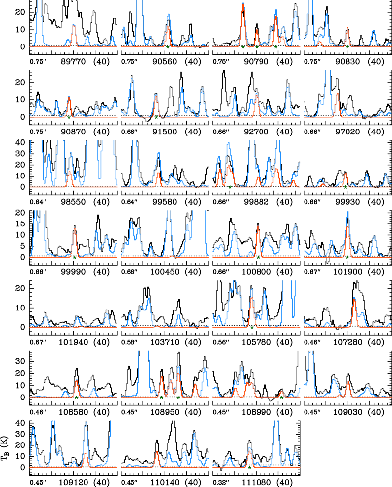
Figure 2: Transitions of NH2CH2CN, $\varv=0$ covered by our ALMA survey. The best-fit LTE synthetic spectrum of NH2CH2CN, $\varv=0$ is displayed in red and overlaid on the observed spectrum of Sgr B2(N1S) shown in black. The blue synthetic spectrum contains the contributions of all molecules identified in our survey so far, including the species shown in red. The central frequency and width are indicated in MHz below each panel. The angular resolution (HPBW) is also indicated. The $y$-axis is labeled in brightness temperature units (K). The dotted line indicates the $3\sigma$ noise level. The green stars mark the aminoacetonitrile lines that we consider as unambiguously detected because they suffer from little contamination by emission from other species.

Table 4: Spectroscopic parameters and integrated intensities of aminoacetonitrile transitions detected toward Sgr B2(N1S) in the ReMoCA survey.

State	Transition	Frequency	$\Delta f$	$A_{\rm ul}$	$E_{\rm u}$	$g_{\rm u}$	$I_{\rm obs}$	$I_{\rm mod}$	$I_{\rm all}$
	$J_{K_{a},K_{c}}$	(MHz)	(kHz)	(10-5 s-1)	(K)		(K km s-1)	(K km s-1)
$\varv=0$	102,9 – 92,8	90561.326	2	2.62	28.9	21	127.9(12)	67.2	137.9
$\varv=0$	106,4 – 96,3	90783.532	2	1.76	68.3	21	169.7(13)	161.3	186.4
$\varv=0$	106,5 – 96,4	90783.532	2	1.76	68.3	21	–	–	–
$\varv=0$	105,6 – 95,5	90784.276	2	2.07	54.8	21	–	–	–
$\varv=0$	105,5 – 95,4	90784.280	2	2.07	54.8	21	–	–	–
$\varv=0$	107,3 – 97,2	90790.252	2	1.41	84.3	21	81.3(12)	54.6	56.0
$\varv=0$	107,4 – 97,3	90790.252	2	1.41	84.3	21	–	–	–
$\varv=0$	104,7 – 94,6	90798.680	2	2.31	43.7	21	159.0(12)	105.6	163.5
$\varv=0$	104,6 – 94,5	90799.244	2	2.31	43.7	21	–	–	–
$\varv=0$	103,8 – 93,7	90829.941	2	2.51	35.1	21	76.2(12)	62.1	63.5
$\varv=0$	103,7 – 93,6	90868.035	2	2.51	35.1	21	73.6(12)	62.1	75.3
$\varv=0$	102,8 – 92,7	91496.111	2	2.71	29.0	21	79.4(12)	65.5	87.1
$\varv=0$	115,7 – 105,6	99869.300	2	2.92	59.6	23	253.4(11)	177.1	349.7
$\varv=0$	115,6 – 105,5	99869.310	2	2.92	59.6	23	–	–	–
$\varv=0$	117,4 – 107,3	99871.145	2	2.19	89.1	23	–	–	–
$\varv=0$	117,5 – 107,4	99871.145	2	2.19	89.1	23	–	–	–
$\varv=0$	113,9 – 103,8	99928.882	2	3.41	39.9	23	88.1(9)	70.5	76.3
$\varv=0$	113,8 – 103,7	99990.564	2	3.42	39.9	23	82.1(9)	70.7	74.1
$\varv=0$	112,9 – 102,8	100800.880	2	3.66	33.8	23	91.6(9)	76.5	79.9
$\varv=0$	111,10 – 101,9	101899.798	2	3.88	30.6	23	117.7(8)	79.0	139.0
$\varv=0$	121,12 – 111,11	105777.967	3	4.36	34.3	25	133.3(12)	87.4	116.8
$\varv=0$	122,11 – 112,10	108581.403	2	4.62	38.9	25	156.5(8)	78.5	86.7
$\varv=0$	126,7 – 116,6	108948.518	3	3.60	78.4	25	135.7(9)	100.3	105.0
$\varv=0$	126,6 – 116,5	108948.518	3	3.60	78.4	25	–	–	–
$\varv=0$	125,8 – 115,7	108956.201	2	3.97	64.8	25	204.4(8)	112.0	148.0
$\varv=0$	125,7 – 115,6	108956.224	2	3.97	64.8	25	–	–	–
$\varv=0$	1210,2 – 1110,1	109001.594	3	1.47	157.1	25	49.7(8)	28.2	29.1
$\varv=0$	1210,3 – 1110,2	109001.594	3	1.47	157.1	25	–	–	–
$\varv=0$	121,11 – 111,10	111076.902	2	5.05	36.0	25	154.7(30)	81.1	111.4
$\varv_{11}=1$	107,3 – 97,2	91000.390	2	1.38	386.8	21	13.5(9)	10.4	13.1
$\varv_{11}=1$	107,4 – 97,3	91000.390	2	1.38	386.8	21	–	–	–
$\varv_{11}=1$	117,4 – 107,3	100102.529	2	2.15	391.6	23	60.7(11)	39.9	48.3
$\varv_{11}=1$	117,5 – 107,4	100102.529	2	2.15	391.6	23	–	–	–
$\varv_{11}=1$	115,7 – 105,6	100104.591	2	2.90	362.3	23	–	–	–
$\varv_{11}=1$	115,6 – 105,5	100104.602	2	2.90	362.3	23	–	–	–
$\varv_{11}=1$	111,10 – 101,9	102166.422	2	3.91	333.7	23	37.1(7)	17.7	26.5
$\varv_{11}=1$	125,8 – 115,7	109213.457	2	3.94	367.6	25	43.5(8)	38.8	51.1
$\varv_{11}=1$	125,7 – 115,6	109213.483	2	3.94	367.6	25	–	–	–
$\varv_{11}=1$	128,4 – 118,3	109214.554	2	2.60	415.2	25	–	–	–
$\varv_{11}=1$	128,5 – 118,4	109214.554	2	2.60	415.2	25	–	–	–
$\varv_{18}=1$	106,5 – 96,4	90906.708	2	1.74	421.4	21	48.4(11)	28.0	32.6
$\varv_{18}=1$	106,4 – 96,3	90906.708	2	1.74	421.4	21	–	–	–
$\varv_{18}=1$	105,6 – 95,5	90906.982	1	2.05	407.6	21	–	–	–
$\varv_{18}=1$	105,5 – 95,4	90906.986	1	2.05	407.6	21	–	–	–

We used the spectroscopic information derived in Sect. 3 to search for rotational transitions from within vibrationally excited states of aminoacetonitrile in the ReMoCA spectrum of Sgr B2(N1S). As a first step, we identified a dozen of transitions of aminoacetonitrile in its vibrational ground state that suffer from little contamination by emission of other species. These detected transitions are marked with a star in Fig. 2 and are listed in Table 4. The best-fit LTE synthetic spectrum that we obtained for aminoacetonitrile is shown in red in Fig. 2 and its parameters are reported in Table 5. Using the same parameters, we could identify four and one rotational transitions from within the vibrationally excited states $\varv_{11}=1$ and $\varv_{18}=1$, respectively. These transitions are marked with a star in Figs. 3 and 4, respectively, and are listed in Table 4.

Table 5: Parameters of our best-fit LTE model of aminoacetonitrile toward Sgr B2(N1S).

Vib.	Status	$N_{\rm det}$	$\theta_{\rm s}$	$T_{\mathrm{rot}}$	$N$	$F_{\rm vib}$	$\Delta V$	$V_{\mathrm{off}}$
state			(′′)	(K)	(cm-2)		(km s-1)	(km s-1)
$\varv=0$	d	18	2.0	200	1.1 (17)	1.00	5.0	0.0
$\varv_{11}=1$	d	4	2.0	200	1.1 (17)	1.00	5.0	0.0
$\varv_{18}=1$	d	1	2.0	200	1.1 (17)	1.00	5.0	0.0
$\varv_{17}=1$	n	0	2.0	200	1.1 (17)	1.00	5.0	0.0
$\varv_{11}=2$	n	0	2.0	200	1.1 (17)	1.00	5.0	0.0

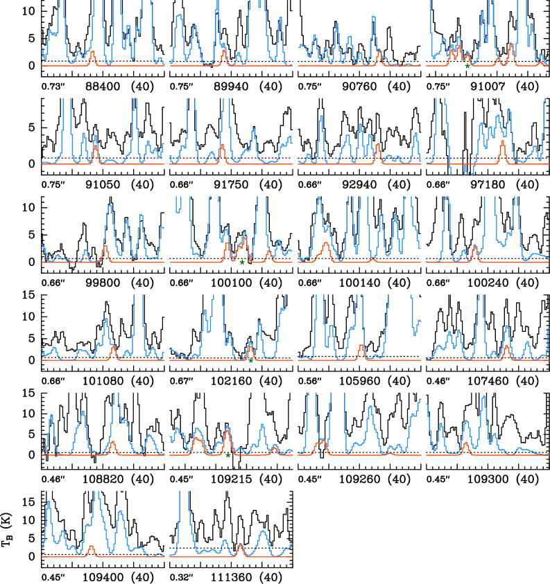
Figure 3: Same as Fig. 2 but for NH2CH2CN, $\varv_{11}=1$.

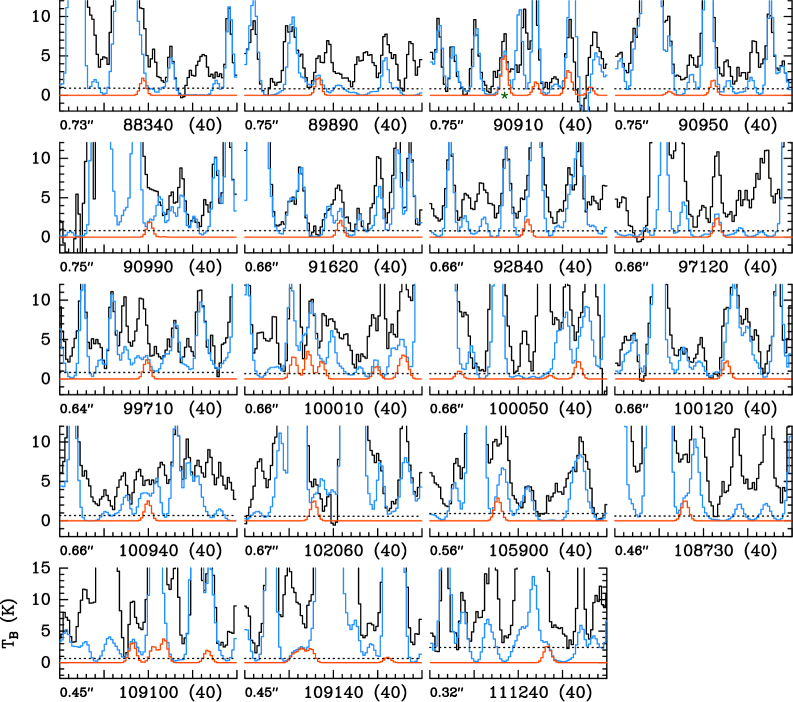
Figure 4: Same as Fig. 2 but for NH2CH2CN, $\varv_{18}=1$.

The model assumes a diameter (FWHM) of 2$\arcsec$ for the emission of aminoacetonitrile, as was done for other species reported by Belloche et al. (2019) toward Sgr B2(N1S). This size is approximately three times bigger than the angular resolution of the ReMoCA survey and thus its exact value does not matter much for the derivation of the column density. A two-dimensional Gaussian fit to the integrated intensity maps of the six least contaminated transitions of aminoacetonitrile yields a mean size of $\sim$1.9$\arcsec$ with an rms dispersion of $\sim$0.15$\arcsec$, consistent with our size assumption.

Using the transitions that are not too much contaminated by emission from other species, we constructed a population diagram for aminoacetonitrile following the same method as Belloche et al. (2016). Figures 5a and b show this diagram before and after correction for optical depth and contamination by emission of other species, respectively. The fit to the population diagram of Fig. 5b yields a rotational temperature of $245\pm 47$ K. As discussed in Sect. 4.4 of Belloche et al. (2019), there are several limitations to this population diagram, in particular because of the non-negligible level of background continuum emission that varies with frequency and angular resolution, and because of the residual contamination of the selected aminoacetonitrile transitions by emission from still unidentified species. These are the reasons why the fitted rotational temperature is uncertain, and its (purely) statistical uncertainty may be underestimated. For the model, we assumed a temperature of 200 K, which yields a good fit to the observed spectrum for both the vibrational ground state and the first two vibrationally excited states (see Figs. 2–4).

There is an inconsistency for one transition of $\varv_{11}=1$ at 109 248 MHz where the synthetic spectrum largely overestimates the observed spectrum (see third panel of fifth row of Fig. 3). This may be due to a blend with absorption lines of ¹³CN produced by translucent or diffuse clouds along the line of sight to Sgr B2 against the strong continuum background of Sgr B2(N1). The $F_{1}$=1-0 multiplet of the $N$=1-0, $J$=1.5-0.5 component of ¹³CN has a rest frequency of $\sim$109 218 MHz and is detected in absorption in the spectrum of Sgr B2(N1S) at the velocity of Sgr B2(N)’s envelope (see the absorption feature in the second panel of the fifth row of Fig. 3, as well as Thiel, 2019). The frequency 109 248 MHz corresponds to a velocity shift of $-82$ km s^-1 with respect to the velocity of Sgr B2(N1S), i.e. a systemic velocity of $-20$ km s^-1 that corresponds to known absorbing clouds in the 4 kpc arm of the Galaxy (Thiel et al., 2019). Therefore, the inconsistency at 109 248 MHz does not invalidate our identification of $\varv_{11}=1$ emission toward Sgr B2(N1S).

We also searched for rotational transitions of aminoacetonitrile from within higher vibrational states, whose spectral predictions were prepared using the newly determined spectroscopic parameters for the $\varv_{17}=1$ state and the constants from Kolesniková et al. (2017) for the $\varv_{11}=2$, $\varv_{11}=\varv_{18}=1$, and $\varv_{18}=2$ states. No transitions of $\varv_{17}=1$ and $\varv_{11}=2$ are unambiguously detected, but some of them contribute significantly to the signal detected with ALMA (see Figs 6 and 7, respectively). While this is not sufficient to claim a detection of these states, we included them in our full model to account for their contribution.

The next two vibrational states, $\varv_{11}=\varv_{18}=1$ and $\varv_{18}=2$, have a few rotational transitions with expected peak intensities at the level of 3–4$\sigma$ according to our LTE model, but they are unfortunately all fully blended with much stronger emission of other species. Therefore, we did not include these states in our full model.

5 Discussion

5.1 Discussion of the spectroscopic results

The analysis carried out in the present paper represents a significant improvement in the spectroscopic knowledge of aminoacetonitrile. Prior to this work, the centrifugal analysis of the aminoacetonitrile spectrum was fairly extensive for the ground state only (Motoki et al., 2013) and more limited for the excited states (Kolesniková et al., 2017; Degli Esposti et al., 2017). Here, this difference has been levelled off for two of the three lowest excited states, the exception being the $\varv_{11}=1$ states whose band is much weaker than the others. Probing energy levels with $J$ up to 80 and $K_{a}$ up to 25, we were able to remarkably extend the centrifugal analysis of aminoacetonitrile; the set of spectroscopic parameters now includes more reliable centrifugal distortion constants as well as additional centrifugal dependencies of the Coriolis term $G_{a}$. Furthermore, in this work we adopted a different choice of fitting parameters with respect to Degli Esposti et al. (2017). This results in a different determination of some spectroscopic constants, which is more pronounced for the purely $K_{a}$-dependent parameters (e.g. $A$, $D_{K}$, and so on).

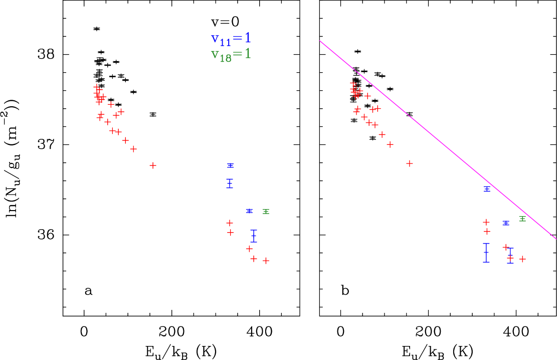
Figure 5: Population diagram of NH2CH2CN toward Sgr B2(N1S). The observed data points are shown in various colors (but not red) as indicated in the upper right corner of panel a while the synthetic populations are shown in red. No correction is applied in panel a. In panel b, the optical depth correction has been applied to both the observed and synthetic populations and the contamination by all other species included in the full model has been removed from the observed data points. The purple line is a linear fit to the observed populations (in linear-logarithmic space).

However, the most important result attained in our analysis is the determination of the vibrational energies of all the three excited states of aminoacetonitrile with relative uncertainties as low as $2\times 10^{-8}$. It has to be noticed that our derived values differs by 2–6  cm^-1 from the energies reported in Bak et al. (1975), where the claimed accuracy was $\pm 1$  cm^-1. Larger discrepancies are found in comparison with low-level theoretical calculations (Bernstein et al., 2004), thus requiring improved levels of theory and approximations to achieve reliable results, as shown e.g. in Melli et al. (2018) for ethanimine. Last, we confidently confirm that the resonance effects between the $\varv_{11}=1$ and $\varv_{18}=1$ states are adequately accounted for and the inclusion of Coriolis interaction parameters is crucial to reproduce the spectrum of aminoacetonitrile. Although the treatment of resonances can be overcome by fitting “effective” spectroscopic parameters (Kolesniková et al., 2017), this approach is not appropriate when spectral prediction must rely on frequency extrapolations of higher $J$ and $K_{a}$ transitions, which might be the case for COMs detected in hot cores.

Our new spectral predictions should be reliable for astronomical identification of aminoacetonitrile from the microwave to the terahertz domain, for both the ground and vibrationally excited states.

5.2 Discussion of the astronomical results

As reported in Sect. 4.2, only four and one spectral lines of $\varv_{11}=1$ and $\varv_{18}=1$, respectively, are found to be little contaminated by emission of other species. While this would not be sufficient to claim the secure detection of a new molecule, the fact that these lines are well reproduced by our LTE model that uses the same consistent set of parameters as the vibrational ground state shows that LTE is a good assumption to describe the level populations of aminoacetonitrile in its vibrational states as well. This gives us strong confidence in the detection of both vibrational states toward Sgr B2(N1S), also because our modelling procedure takes into account the contribution of all identified molecules and thus reduces the risks of misassignments.

The column density of aminoacetonitrile derived from our LTE modelling of the ReMoCA spectrum toward Sgr B2(N1S), $1.1\times 10^{17}$ cm^-2, is 3.9 times higher than the column density reported in Belloche et al. (2008) for Sgr B2(N) from observations with the IRAM 30 m telescope, although in both cases we assumed the same emission size. There are several reasons for this difference. First of all, Belloche et al. (2008) did not account for the contribution of the vibrational partition function. At the temperature they assumed, 100 K, this contribution amounts to a factor 1.09 and, accounting for this, the column density derived from the IRAM 30 m data becomes $3.0\times 10^{16}$ cm^-2. Second, the column density of Belloche et al. (2008) was computed at 100 K while here we used a temperature of 200 K. Assuming a temperature of 100 K like Belloche et al. (2008) would underestimate the intensities of the higher-energy transitions detected in the ReMoCA spectrum but we would obtain a column density of $\sim$$4.3\times 10^{16}$ cm^-2 on the basis of the lower-energy ones. Finally, the column density derived here characterizes the position Sgr B2(N1S) only, as probed with an angular resolution of 0.6$\arcsec$. At this scale, the velocity dispersion of the aminoacetonitrile emission is 5 km s^-1, somewhat smaller than the velocity dispersion probed with the 30 m telescope (7 km s^-1). Spatial variations across the hot core Sgr B2(N1), completely covered by the single-dish beam, and calibration uncertainties could explain the remaining $\sim$30% discrepancy.

5.3 Formation of aminoacetonitrile

The interstellar chemistry of aminoacetonitrile was first simulated by Belloche et al. (2009), who incorporated it into their gas-grain chemical network along with new chemistry for n-propyl cyanide, ethyl formate, and other species related to all three. The network they developed for aminoacetonitrile, as with other complex organics, relied on grain-surface/ice chemistry to produce the molecule from simpler, more abundant building blocks at low to intermediate temperatures, with the aminoacetonitrile produced on the grains ultimately being released into the gas phase at typical hot-core temperatures greater than $\sim$100 K. A selection of ion-molecule destruction routes for gas-phase aminoacetonitrile were also included.

Building on this network to include glycine-related chemistry, Garrod (2013) employed a three-phase model of hot-core chemistry, in which the ice-surface and bulk were treated independently. This model included a selection of other updates and improvements to the treatment of surface/bulk chemistry; we therefore discuss the later results in preference, although in fact the general behavior of the aminoacetonitrile chemistry is not too dissimilar between the two models.

The current understanding of aminoacetonitrile production, based on astrochemical kinetic models, therefore assumes production on grains. Garrod (2013) finds that it is predominantly formed through the addition of the radicals NH2 and CH2CN within and upon the ice mantles, although another radical-addition process, between NH2CH2 and CN, is also present in the network and makes a modest contribution. The radicals themselves are produced by direct photodissociation of stable, solid-phase species such as ammonia and methyl cyanide, or through the abstraction of hydrogen from those species by reactive and abundant radicals like OH, which itself is formed through the photodissociation of water. This photodissociation is caused by the weak, secondary UV field induced by cosmic-ray collisions with gas-phase H2. Garrod (2013) also discerned an increase in aminoacetonitrile production associated with the thermal desorption of methyl cyanide, whose gas-phase destruction routes included production of the CH2CN radical; the latter species could produce aminoacetonitrile by re-accreting onto the grain/ice surface and there reacting with NH2.

Both chemical models produced fractional abundances with respect to H2 on the order of $10^{-8}$. Comparing the peak aminoacetonitrile abundance with that of methanol obtained in the medium warm-up timescale model of Garrod (2013) provides a ratio $\sim$$1.3\times 10^{-3}$. Based on the column density data obtained in the present work, and using an observational methanol column density of $2.0\times 10^{19}$ cm^-2 for Sgr B2(N1S) (Motiyenko & et al., 2020), an observational ratio of $5.5\times 10^{-3}$ is found. The models therefore appear roughly consistent with the observations, suggesting that photochemistry within the ices remains a plausible formation route for aminoacetonitrile.

6 Conclusions

We presented a combined spectroscopic and observational study of vibrationally excited aminoacetonitrile, a species considered closely related to amino acids. The high-resolution far-infrared spectrum of aminoacetonitrile has been recorded for the first time using a synchrotron-based FT spectrometer. Three bands were observed in the frequency region between 100 and 500  cm^-1, corresponding to the CCN bending ($\nu_{11}$), NH2 torsion ($\nu_{18}$), and CH2-NH2 torsion ($\nu_{17}$) modes. Then, rotational signatures from aminoacetonitrile in the ground and vibrationally excited states was searched for in the ReMoCA imaging spectral line survey of Sgr B2(N). A number of 23 lines with lower energy levels ranging from 29 to 422 K were detected in emission around 3 mm toward the main hot core. The main results of this work can be summarized as follows:

1. The energies of the $\varv_{11}=1$, $\varv_{18}=1$, and $\varv_{17}=1$ vibrationally excited states of aminoacetonitrile have been accurately determined from the analysis of almost 11 000 ro-vibrational lines and around 2 000 rotational data.

2. Updated catalog entries of aminoacetonitrile in its ground and vibrationally excited states have been produced using the newly evaluated values of the vibration-rotation partition function together with the new set of spectroscopic constants.

3. We report the interstellar detection of aminoacetonitrile in its vibrational states $\varv_{11}=1$ and $\varv_{18}=1$ toward the main hot core of Sgr B2(N), with intensities consistent with expectations from an LTE model that fits well the emission of aminoacetonitrile in its vibrational ground state.

4. The next two vibrational states, $\varv_{17}=1$ and $\varv_{11}=2$ contribute significantly to the observed spectrum, but cannot be identified securely due to blends with emission from other species. The next two states, $\varv_{11}=\varv_{18}=1$ and $\varv_{18}=2$ are not detected.

This work demonstrates that a strong interplay between laboratory spectroscopy exploiting (sub)millimeter and synchrotron far-infrared techniques, and observational spectral surveys can lead to the detection of COMs in space and quantify their abundances. Future projects concerning the recording and analysis of infrared bands of aminoacetonitrile at frequencies higher than 500 cm^-1 are planned.

Appendix A Complementary figures: Spectra

Figures 6 and 7 show rotational transitions of aminoacetonitrile from within its vibrationally excited states $\varv_{17}=1$ and $\varv_{11}=2$, respectively, that are covered by the ReMoCA survey. Some of them significantly contribute to the signal detected toward Sgr B2(N1S).

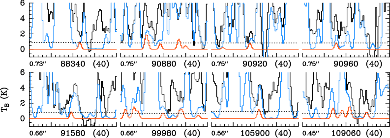
Figure 6: Same as Fig. 2 but for NH2CH2CN, $\varv_{17}=1$.

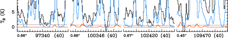
Figure 7: Same as Fig. 2 but for NH2CH2CN, $\varv_{11}=2$.