Dynamically Mitigating Data Discrepancy with Balanced Focal Loss for Replay Attack Detection

Abstract

It becomes urgent to design effective anti-spoofing algorithms for vulnerable automatic speaker verification systems due to the advancement of high-quality playback devices. Current studies mainly treat anti-spoofing as a binary classification problem between bonafide and spoofed utterances, while lack of indistinguishable samples makes it difficult to train a robust spoofing detector. In this paper, we argue that for anti-spoofing, it needs more attention for indistinguishable samples over easily-classified ones in the modeling process, to make correct discrimination a top priority. Therefore, to mitigate the data discrepancy between training and inference, we propose D3M, to leverage a balanced focal loss function as the training objective to dynamically scale the loss based on the traits of the sample itself. Besides, in the experiments, we select three kinds of features that contain both magnitude-based and phase-based information to form complementary and informative features. Experimental results on the ASVspoof2019 dataset demonstrate the superiority of the proposed methods by comparison between our systems and top-performing ones. Systems trained with the balanced focal loss perform significantly better than conventional cross-entropy loss. With complementary features, our fusion system with only three kinds of features outperforms other systems containing five or more complex single models by 22.5% for min-tDCF and 7% for EER, achieving a min-tDCF and an EER of 0.0124 and 0.55% respectively. Furthermore, we present and discuss the evaluation results on real replay data apart from the simulated ASVspoof2019 data, indicating that research for anti-spoofing still has a long way to go. Source code, analysis data, and other details are publicly available at https://github.com/asvspoof/D3M.

I Introduction

Figure 1: An example for comparison between a bonafide utterance and its corresponding spoofed utterances with different attack types, illustrates that high-quality attack AA has only subtle differences from the bonafide one, yet taking up a small portion of the data. We term this phenomenon as data discrepancy in anti-spoofing, and propose a method to replace the conventional balanced cross-entropy loss (BCE) with the novel balanced focal loss (BFL) as the training objective. It is worth noting that hard and easy samples do not have strict boundaries, nor will there be a certain attack method as the dividing line, which demonstrates the necessity of making dynamic adjustments with BFL. The MGD-gram feature is used for visualization, see Fig.4 for high-resolution visualization. Description of different attack types (AA, AB, AC) and analysis are elaborated in Section V-B and Fig. 4, respectively. Best viewed in color.

Automatic Speaker Verification (ASV), intended for authenticating a claimed speaker identity by characteristics of the voice, has shown promising results recently. With rapid advancement of ASV and its wide applications such as smart assistants and banking systems, vulnerability of ASV systems has been gradually exposed. More specifically, current ASV systems have almost no defense against spoofing attacks (also known as presentation attacks). According to possible attack locations in a typical ASV system (ISO/IEC 30107), spoofing attacks can be categorized into four major classes: (i) impersonation, (ii) speech synthesis, (iii) voice conversion and (iv) replay. The first three classes rely on professional knowledge heavily, while replay attack does not require any kind of expertise. Besides, easy access to high-quality playback devices makes it even more urgent to develop robust anti-spoofing systems against replay attack, which is also the goal we strive for in this work.

Thanks to the impetus injected by the 2015, 2017 and 2019 ASVspoof Challenges, great achievements have been made by numerous researchers in the past few years. In 2017, replay attack detection was first introduced to the challenge with the aim of measuring limits and developing countermeasures. Simultaneously, deep learning-based approaches came to the fore [1]. The ASVspoof2019 Challenge extended the previous challenge with improved, controlled simulation and start-of-the-art spoofing methods for generating replay data, as well as new primary evaluation metric t-DCF [2]. Such anti-spoofing systems as [3] and [4] ranked among the best systems, leading to two lines of work for deep learning-based architectures. One is based on LightCNN, and the other is based on ResNet [5].

Current state-of-the-art anti-spoofing systems mainly suffer from two challenges. On the one hand, there exists discrepancy in data distribution among training, testing, evaluation and real data, which has a great impact on the model performance. Similar to image classification, previous studies like [6, 7] regard the data discrepancy as a class-imbalance problem. Widely-adopted strategies to solve the class-imbalance problem can be divided into re-sampling and re-weighting [8]. Re-sampling strategies, including over-sampling and under-sampling, are complicated and have drawbacks such as incurring risks from removing important samples. Compared with re-sampling, re-weighting strategies are relatively simple and based on the statistics of data, for example, use the inverse of class frequency as the weighting factor [6]. For replay attack detection, we argue that, the main challenge lies in the data discrepancy and it cannot only be viewed as class-imbalance problems of binary classification[6] or multi-class classification [4] in a narrow sense. Strategies for the imbalance of different classes place more emphasis on the inter-class fairness, while for data discrepancy, more emphases are needed for easily-misclassified indistinguishable samples, which only take up a small portion in the training data, but are the overriding factors as the attack sources come from increasingly accessible quality devices[9, 8]. Therefore, a dynamically re-weighting training objective becomes a crucial driving force to bridge the gap. On the other hand, the need to select informative feature representations arises when building a system with a growing number of features. As a consequence, choosing fewer but sufficient, complementary features is of supreme importance [10]. In this paper, we focus on resolving the two challenges mentioned above, especially the first one. Our main contributions can be summarized as follows:

1. Inspired by [9], we propose a Dynamic Data Discrepancy Mitigation method (D3M) that leverages balanced focal loss as a novel training objective for anti-spoofing, which enables the model to attend more to indistinguishable samples with dynamically scaled loss value. Through detailed analysis, we find that balanced focal loss outperforms other baselines to a large extent. To our knowledge, we are the first to introduce focal loss to anti-spoofing, mitigating the data discrepancy between training and inference.

2. Based on our survey of the ASVspoof2019 Challenge, only group delay (GD) was used by researchers as phased-based features. We extend the ideas from [11] to first investigate the performance of the modified group delay function [12], dubbed MGD-gram, on the improved ASVspoof2019 dataset which uses start-of-the-art spoofing methods for generating replay data. Also, we demonstrate the superiority of fusion of three kinds of complementary features, namely modified group delay (MGD) gram, short-time Fourier transform (STFT) gram and constant Q transform (CQT) gram.

3. We show that the performance of current top-performing systems on real data are not as good as on the simulated ASVspoof2019 data [13], which is unexpected and considered very worthy of discussion. This may be due to the fact that simulated data cannot be applied to real cases, or the distinctions between GMM and ConvNets. Deep learning-based methods for anti-spoofing still have a long way to go, as the conventional GMM model has the best performance, although it is not good enough, with an EER of 12.4%.

II Cost-Sensitive Training — the Balanced Focal Loss

Almost all the anti-spoofing systems have poor performance for samples made by replay devices with higher quality and a shorter attacker-to-talker distance. These indistinguishable samples can be easily misclassified, thus posing a severe threat to anti-spoofing systems. Moreover, indistinguishable samples only take up a small portion of the training data, making the recognition extremely harder because the training procedure is dominated by the majority. Specifically, for gradient-based methods like neural networks, the gradients are dominated by easy samples.

We term the above phenomenon as the data discrepancy between training and inference in anti-spoofing. Unlike image classification or object detection suffering from class-imbalance, data discrepancy faced in anti-spoofing is a more severe challenge, which emphasizes more on the correctness of discrimination and the security of the biometric system than just on the fairness between different classes of attacks.

To mitigate this problem, on the basis of the common strategy to solve class imbalance, i.e. simple re-weighting (balancing by class frequency), we further propose to leverage BFL as the training objective instead of BCE. Focal loss was first used in the field of object detection, and its validity has been tested on many tasks [9].

We use the example shown in Fig. 1 to illustrate our idea. As shown in Fig. 1, only subtle differences exist with red marks for the sample of attack type AA, compared with other two samples of “easier” attack types such as AB and AC.

Intuitively, to increase the accuracy for harder samples of attack type AA, we need to make the system pay more attention to them during training. Therefore, simply by assigning bigger loss values to harder samples and smaller values to easier examples, we can achieve our goal.

Formally, the balanced focal loss, a weighted variant of the standard focal loss, can be calculated as:

$$\mathrm{BFL}\left(p_{\mathrm{t}}\right)=-\alpha_{\mathrm{t}}\left(1-p_{\mathrm{t}}\right)^{\gamma}\log\left(p_{\mathrm{t}}\right),$$ (1)

where subscript $\mathrm{t}$ refers to the true class label, and $\alpha$ denotes the weight for the corresponding class to mitigate the class-imbalance problem, and $\gamma$ is tunable as a focusing parameter to control the relative scaling. We find $\gamma=2$ best in the experiments (the red curve in the Fig. 1).

Both BFL and BCE use $\alpha_{t}$ (the inverse of class frequency) to statically re-weight the loss. The main difference between BFL and BCE is that BFL uses an additional weighting factor $\left(1-p_{\mathrm{t}}\right)^{\gamma}$ to dynamically scale the value of the contribution of each sample to the final loss, based on the probability of target label $p_{\mathrm{t}}$ and a focusing factor $\gamma$, so as to focus more on indistinguishable samples and reduce the relative loss for easily-classified samples, as illustrated in Fig. 1. It is worth noting that since $p_{\mathrm{t}}$ is the probability of the target label predicted by the weight, using $\left(1-p_{\mathrm{t}}\right)^{\gamma}$ to scale the loss is like performing a soft attention.

III The Model Architecture — End-to-end Residual Network

TABLE I: The network structure used in this paper. The input feature size is (1, 513, 500). Any two convolutional layers have batch normalization followed by the ReLU activation function in between. Global average pooling is used between the last convolutional layer and the fully-connected layer.

Layer	Filter	Output shape	# Params.
Conv2d	3x3,1	(16, 513, 500)	144
Max Pooling	–	(16, 513, 500)	–
ResBlock1 x 3	3x3,16	(16, 513, 500)	4.6k x 3
ResBlock2 x 4	3x3, 32	(32, 257, 250)	18.4k x 4
ResBlock3 x 6	3x3, 64	(64, 129, 125)	73.7k x 6
ResBlock4 x 3	3x3, 128	(128, 65, 63)	295.0k x 3
GAP	–	(128, )	–
FC	32	(32, )	4.1k
Output	2	(2, )	66

Recently, with great progress made by researchers participating in the 2015, 2017 and 2019 ASVspoof challenges, LightCNN-based and ResNet-based deep neural networks have become the mainstream as high-level feature extractors [1, 3, 4]. As mentioned earlier, instead of proposing a novel network architecture, this work mainly aims to present informative feature representations and the effective training objective. Hence, we select the ResNet-based end-to-end model as the backbone, making use of its superior extracting and modeling capabilities.

As illustrated with detailed configurations in Table I, our model is similar to [7]. The main differences are: (i) fixed-length feature representations are used, and features are either padded or truncated to n_frames = 500 along the time axis according to statistics derived from data, whereas in [7], the model takes fixed-length input utterances for training and variable-length utterances for test. The purpose of our modification behind is to facilitate the training process while maintaining consistency during training and inference; (ii) all the models are trained from scratch with no modification of data, that is, we use neither data augmentation nor pre-trained techniques.

The final countermeasure score, representing the genuineness judgement for each utterance provided by the system, is calculated as the log-likelihood ratio using Eq. (2),

$$s_{cm}(utt)=\log(p(\text{bonafide}|utt;\theta))-\log(p(\text{spoof}|utt;\theta))$$ (2)

where $utt$ refers to a test utterance, and $\theta$ denotes model parameters. This is also a recommended method for score computation by the ASVspoof2019 Commmittee. The probabilities of bonafide and spoofed speech utterances are given by the final softmax layer of the model.

IV Integration of Complementary Features

Magnitude-based information included in short-time Fourier transform gram has been widely used in top-performing anti-spoofing systems such as [4] and [6], while features containing phased-based information used in [11] and [7] also yield superior performance. However, in the ASVSpoof2019 Challenge, we find that only GD-gram was used by researches as phased-based time-frequency representation, although Modified GD feature has been proved effective in the previous work [14, 15]. To further investigate their performance on the improved ASVSpoof2019 dataset, we compare MGD-gram with GD-gram in out experiments. Both of them are low-level time-frequency representations, which can better utilize the modeling capabilities of the ResNet neural network. Besides, to integrate complementary features, in this paper, we carefully explore three different kinds of features, namely MGD-gram, STFT-gram and CQT-gram. We employ the MGD-gram and STFT-gram to integrate both magnitude and phase information. Also, the CQT-gram, shown in [16] to yield a superior performance to general forms of spoofing attack with higher frequency resolution in the lower frequency(?), is added to them to form complementary informative feature representations.

IV-A Modified Group Delay Gram (MGD-gram)

In [11, 7], the group delay function, defined as the negative derivative of phase, was used to characterize speech signals to distinguish bonafide utterances from spoofed ones on the ASVspoof2019 dataset.

As clearly illustrated in [17], the vanilla group delay function suffers from its spiky nature and requires the signal be a minimum phase. However, speech segments can be non-minimum due to zeroes from windowing and noise. The MGD function is thus proposed as a parameterized and improved version of the GD function, which is formulated using [12]:

$$\tau_{m}(\omega,t)=\left(\frac{\tau(\omega,t)^{\prime}}{|\tau(\omega,t)^{\prime}|}\right)(|\tau(\omega,t)^{\prime}|)^{\rho},$$ (3)

where

$$\tau(\omega,t)^{\prime}=\left(\frac{X_{R}(\omega,t)Y_{R}(\omega,t)+Y_{I}(\omega,t)X_{I}(\omega,t)}{S(\omega,t)^{2\lambda}}\right),$$ (4)

where $S(\omega,t)$ is the cepstrally smoothed version of $|X(\omega,t)|$, and $\rho$ and $\lambda$ are newly added parameters to reduce the aforementioned spikes ($0<\rho\leq 1.0$ and $0<\lambda\leq 1.0$).

After replacing the GD function with the MGD function, we can easily get the MGD-gram representation by concatenating all the frames’ outputs.

IV-B Short-time Fourier Transform Gram (STFT-gram)

The short-time Fourier transform (STFT) [18] was proposed to solve the problem that the Fourier transform cannot reflect local features of a signal. The utterances are first broken up into overlapping frames and then the Fourier transform is performed on each short frame, forming a 2-D complex matrix finally. STFT converts a time domain signal into a frequency domain signal. STFT-gram (also know as spectrogram) is one of the most widely-used features now, which contains magnitude-based information. In [4], many systems achieved great performance with STFT-gram. As a result, we choose STFT-gram as one of our complementary features.

IV-C Constant Q Transform Gram (CQT-gram)

The constant Q transform (CQT) [19] employs geometrically spaced frequency bins to make the constant Q factor across entire spectrum. CQT was designed to resolve problems for musical temperament as it can give the same frequency as the scale frequency. Simultaneously, CQT performs well for automatic speaker verification with a higher frequency resolution at lower frequencies and a higher temporal resolution at higher frequencies, which enables it closer to human perception. Thus, we incorporate CQT-gram into our complementary features. We apply CQT on the utterance, and log transform is followed to derive the CQT-gram.

IV-D Fusion Scheme

In our experiments, we train three models that have identical model architecture with aforementioned features, and later fuse their scores by taking the average (mean-fusion) and employing logistics regression (LR). Note that we strictly follow the evaluation protocol from the ASVspoof2019 Challenge [13].

V Experiments & Analysis

Experiments in this study were conducted using PyTorch [20], a deep learning library in Python. Source code and other details are publicly available at https://github.com/asvspoof/D3M.

V-A Baseline Systems

Offical Baselines: We adopt the officially two baseline models together with the dataset released by the ASVspoof 2019 Committee. These two systems are based on the same conventional 2-class GMM backend with 512 components and two kinds of acoustic features, namely linear frequency cepstral coefficients (LFCC) and constant Q cepstral coefficients (CQCC). Details can be found in [13].

Top-performing NN-based Models: According to the challenge results reported in [5], many top systems employ neural network(NN)-based models. To further test the performance of our proposed methods, we choose the newly published systems ranked 3rd sidual architectures to our NN-based baseline models [4, 7]. The top-1 system of this challenge has not been publicly available yet, and the top-2 system is a LightCNN based one with some modifications on feature sizes which is not very suitable for comparison. Specifically, we adopt the ResNet architecture trained with the balanced cross-entropy loss as our baseline models [7]. Note that in order to control variables, we further re-implemented the work in [7] under the same settings with a similar network architecture.

V-B Settings

Datasets:

The ASVspoof2019 simulated PA dataset [13], an improved version with controlled environments and acoustic configurations of the dataset of 2017, can be divided into three subsets: the training set (PA train set), the development set (PA dev set), and the evaluation set (PA eval set).

In addition to the simulated PA subsets, we use the Real-PA dataset, recently released by the ASVspoof committee [13], which was made with real replay operations from three different labs, to further test the performance of anti-spoofing systems. Note that the real data contains additive noise, which is not contained in the simulated PA subsets. As a consequence, spoofing detection results on the real replay data are not expected to be as good as those obtained from the simulated PA subsets, but we can still get some insights by comparing conventional methods with deep learning-based methods.

Details about the simulated PA datasets and the Real-PA dataset are illustrated in Table II and Table III.

TABLE II: Statistics of datasets used in this work

Datasets	# Bonafide utterances	# Spoofed utterances
PA train set	5,400	48,600
PA dev set	5,400	24,300
PA eval set	18,090	116,640
Real-PA set	540	2,160

TABLE III: Detailed information of different attack sources

	A	B	C
Attacker-to-talker distance $D_{a}$ (cm)	$10-50$	$50-100$	$>100$
Replay device quality $Q$	perfect	high	low

TABLE IV: Overall Performance of different systems on the ASVspoof2019 PA eval set. We experimented with mean-fusion and logistic regression (LR) fusion for models that use three kinds of features all trained with BCE or BFL. The BFL + LR Fusion achieves the best performance with only three single models. Better generalization ability of the proposed methods could be seen, i.e. reduced overfitting on the PA Dev Set.

Method	System	# Models	PA Dev Set		PA Eval Set
			t-DCF${}_{norm}^{min}$	EER(%)	t-DCF${}^{min}_{norm}$	EER(%)
Official Baseline	LFCC+GMM	-a	0.2554	11.96	0.3017	13.54
	CQCC+GMM	-	0.1953	9.87	0.2454	11.04
[7]	Fusion System	6	0.0064	0.24	0.0168	0.66
[4]	Fusion System	5	0.0030	0.13	0.0160	0.59
D3M (This work)	BCE + Mean Fusion	3	0.0092	0.40	0.0153	0.62
	BCE + LR Fusion	3	0.0084	0.37	0.0151	0.61
	BFL + Mean Fusion	3	0.0075	0.35	0.0127	0.56
	BFL + LR Fusion	3	0.0077	0.35	0.0124	0.55

• The official baseline adopts conventional methods and therefore does not participate in the comparison of the number of neural networks used for model ensemble.

Feature Extraction: We use the following configurations to extract features:

• STFT-gram: STFT spectrum was extracted with 25-ms frame length and 10-ms frame shift. The number of FFT bins was set to 1,024. Spectrums of all the frames were then concatenated to form STFT-gram.

• MGD-gram: Tuned on the development set, the parameters of the MGD function were empirically set to $\rho=0.2$ and $\lambda=0.7$. The number of FFT bins was 1,024.

• CQT-gram: CQT spectrum was extracted with a hop length of 128 sample points. The number of octaves and the number of bins per octave $b$ were set to 9 and 96, respectively.

Training Scheme: The networks were optimized by the AdamW optimizer [21], with parameter settings $\beta_{1}=0.9$, $\beta_{2}=0.999$, and weight decay 5e-5, which can substantially improve the generalization performance of the widely-used optimizer Adam. Besides, scheduler ReduceLROnPlateau in PyTorch was employed with max_patience = 3 and reduce_factor = 0.1 to reduce the learning rate once learning stagnated.

Evaluation Metrics:

• Tandem detection cost function (t-DCF) : Introduced in the ASVspoof2019 Challenge, t-DCF reflects the influence of spoofing countermeasure (CM) performance on ASV reliability under the same analysis framework [2]. We adopt the t-DCF as the primary evaluation metric.

• Equal Error Rate (EER): Determined by adjusting the threshold to make the false rejection rate (FRR) equal to false acceptance rate (FAR), EER is used as the secondary evaluation metric in our experiments, which is suitable for measuring the performance of a single anti-spoofing or ASV system.

V-C Evaluation Results on the ASVspoof2019 PA Eval Set

V-C1 Overall Performance

Table IV gives our overall performance on the PA eval set. We compare our models with the top-performing systems [7] and [4] ranked 3rd and 4th in the 2019 challenge. Instead of these baseline models with five or more complex single models, our best fusion system outperforms them with only three single models, which is simple and computationally efficient. The results on the PA dev set and PA eval set also demonstrate the effectiveness of the balanced focal loss that focuses on harder samples to mitigate the discrepancy of data distributions between training and inference and make a model more generalizable.

V-C2 Results on MGD-gram vs GD-gram

TABLE V: Performance of MGD-gram vs GD-gram under different configurations on the ASVspoof2019 PA dev set. No other tricks like data augmentation were used in our experiments.

Feature	Model	t-DCF${}^{min}_{norm}$	EER(%)
GD-gram	ResNet w BCE	0.0467	1.81
MGD-gram	ResNet w BCE	0.0288	1.07
MGD-gram	ResNet w BFL	0.0257	1.04

The results in Table V show that MGD-gram is significantly better than GD-gram (by 40.9%) as a kind of feature representation. Comparison in Table V also verifies the effectiveness of the balanced focal loss. More detailed evaluation results for BFL will be reported in later subsections.

V-C3 Single Models

TABLE VI: Performance of different single models on the ASVspoof2019 PA eval set. EM refers to the expectation maximization algorithm for the GMM model training.

Method	Model	Training Objective	PA Dev Set		PA Eval Set
			t-DCF${}_{norm}^{min}$	EER(%)	t-DCF${}^{min}_{norm}$	EER(%)
[7]	ResNet+GD-gram	BCE	0.0467	1.81	0.0439	1.79
[4]	SENet+STFT-gram	BCE	0.0150	0.58	0.036	1.29
D3M (This work)	ResNet+STFT-gram	BCE	0.0131	0.65	0.0261	1.12
	+STFT-gram	BFL	0.0163	0.63	0.0251	1.01
	ResNet+MGD-gram	BCE	0.0288	1.07	0.0396	1.57
	+MGD-gram	BFL	0.0257	1.04	0.0343	1.39
	ResNet+CQT-gram	BCE	0.0445	1.87	0.0477	2.02
	+CQT-gram	BFL	0.0393	1.80	0.0465	1.89

As shown in Table VI, on the PA eval set, for single models, all the deep learning-based models achieve better performance than the conventional GMM models. In the ASVspoof2019 Challenge, [7] proposes to model speech characteristics using the ResNet architecture [22] and phase-based GD-gram features. [4], using STFT-gram as the feature input, employs SENet which contains squeeze and excitation operations to facilitate the feature extraction and explicitly model the importance of different feature channels. Compared with them, our single models, with a similar architecture to [7] and features introduced in Section IV, show competitive results. It is worth mentioning that the number of parameters in our models is less than that of [4].

Comparing our models trained with BFL and BCE, we find that models equipped with BFL as the training objective significantly outperform those with BCE. Taking the ResNet+MGD-gram as an example, BFL improves the min-tDCF and EER by 12.6% and 11.5%, respectively. The ResNet+STFT-gram+BFL model achieves the overall best performance and shows a better generalization ability in terms of the results on the PA dev set and the PA eval set when compared with SENet+STFT-gram in [4]. Detailed analysis for the effectiveness of the training objective with respect to each attack type will be reported in Subsection V-D.

V-D Effectiveness of the Training Objective

In this subsection, we present detailed performance analysis for the training objective with the results of the single models and fusion systems over nine attacks.

To make detailed analysis for the effectiveness of the training objective, we divide the PA Eval Set into nine parts based on the types of spoofing attack information, corresponding to nine different spoofing methods: AA, AB, AC, BA, BB, BC, CA, CB, and CC. We experiment with single attacks and then plot the score statistics in Fig. 2 and Fig. 3.

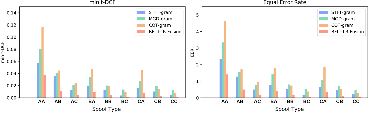
Figure 2: Detailed evaluation results over nine attack types for single models and the best fusion system BFL + LR Fusion in terms of min-tDCF and EER. All the single models are trained with BFL. Best viewed in color.

As shown in Fig.2, the three complementary independent models using BFL and the fusion system that combining these three have a good ability to discriminate against every type of spoof information, and for types that are more difficult and closer to the bonafide ones such as AB, BA, and CA, those trained with BFL still have strong ability to distinguish the bonafide and spoofed utterances. In particular, for type AA, which is almost indistinguishable from bonafide utterances, the system using BFL also achieves lower min-tDCF and EER.

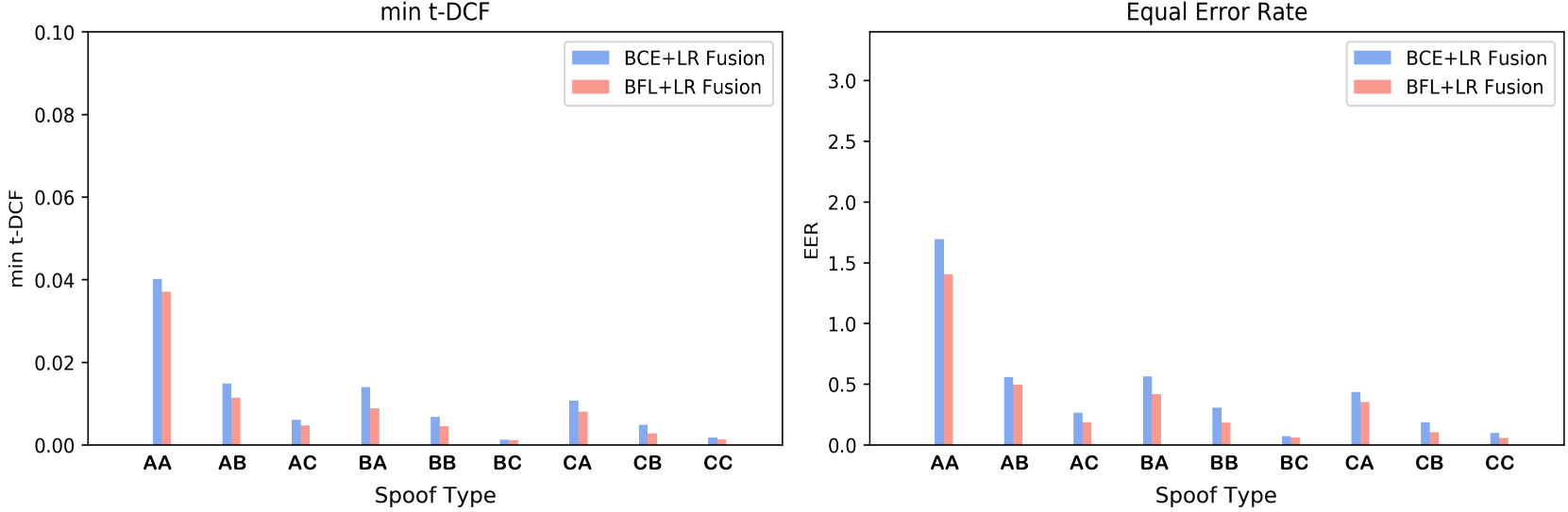
Figure 3: Comparision of fusion systems BCE+LR Fusion and BFL+LR Fusion based on the balanced focal loss and cross-entropy loss in terms of min-tDCF and EER over nine attack types. Best viewed in color.

Fig.3 shows the performance of two fusion systems with two different loss functions over nine types of spoofing attack methods. As can be seen from this figure, the use of BFL makes BFL+LR Fusion perform much better than BCE+LR Fusion. It is worth mentioning that for the quality attack samples of type AA, which is difficult to distinguish, the fusion system using BFL is more distinguishable than the fusion system using the widely-used balanced cross-entropy loss. This also reflects the robustness and generalization ability of the BFL+LR Fusion system, dynamically focusing more on indistinguishable samples.

V-E Understanding the Network Decisions with Saliency Maps via Backpropagation

To better understand how the network make its classification decisions and verify our original motivation of leveraging BFL as the proper training objective to solve the data discrepancy problem, we further visualize the the original features and their corresponding saliency maps via backpropagation [23], an efficient way of network visualization. As shown in Fig. 4, the magnitudes of saliency maps are decreasing from quality attack type AA to relatively easy type AC. The decreasing gradient magnitude, together with increasing amount of hot “pixels” (time-frequency bins), verifies the initial intuition (see Fig.1) and demonstrates the necessity of our proposed method.

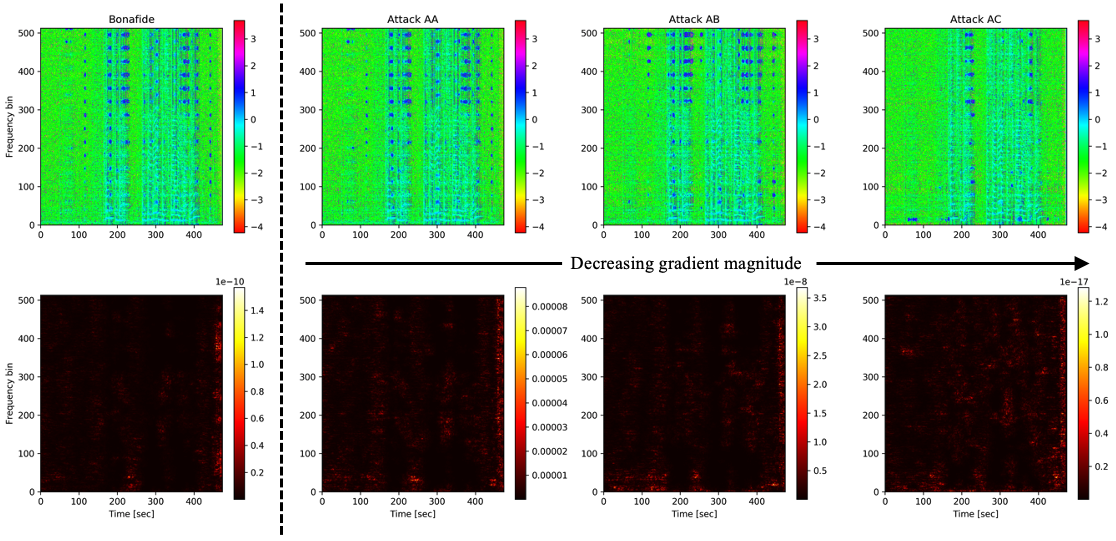
Figure 4: Visualization of original features (Top) vs. saliency maps (Bottom) via backpropagation to better understand critical parts for the network’s making classification decisions. Hotness corresponds to regions that have a big impact on the final decisions. Decreasing gradient magnitude and increasing amount of hot pixels (time-frequency bins) verified the proposed idea, since higher gradient magnitude of harder attack types, with fewer amount of hot pixels, implies more decision sensitivity to value changes in corresponding pixels for utterances generated by quality attacks, hence these samples are harder.

V-F Evaluation Results on the Real-PA Set

TABLE VII: Performance of different systems on the ASVspoof2019 Real-PA set. For fusion systems, only the result of the best (Mean-Fusion) is reported in this table.

System	Training Objective	EER(%)
LFCC+GMM	EM	28.92
CQCC+GMM	EM	12.40
ResNet+STFT-gram	BCE	46.85
+STFT-gram	BFL	51.50
ResNet+MGD-gram	BCE	23.91
+MGD-gram	BFL	29.86
ResNet+CQT-gram	BCE	30.95
+CQT-gram	BFL	23.56
Mean-Fusion	BFL	25.02

The performance of different systems on the ASVspoof2019 Real-PA set are shown in Table VII. To our knowledge, we are the first to report the evaluation results on the recently-released Real-PA dataset [13], and unexpected experimental results are shown which are worthy of discussion. We can observe that current top-performing systems on real data are not as good as on the ASVspoof2019 simulated PA dataset. Although there is additional noise in the Real-PA set which is not contained in the simulated PA dataset, conventional GMM models still perform best. The performance degradation may be due to the fact that simulated data cannot match real scenarios completely. Another possible reason may be the time-frequency distortions captured by CNN-based methods like ResNet are not detected by the time-level GMM model, which also needs further analysis and improvement.

VI Conclusions

This paper aimed at resolving two challenges when designing replay attack detection systems. Firstly, we proposed D3M to leverage the novel balanced focal loss to dynamically mitigate the discrepancy of the data distributions between training and inference. We then presented the experiments with MGD-gram and selected complementary features on the ASVspoof2019 dataset. Experimental results and detailed analysis verified the effectiveness of the proposed methods by comparing them with the top-performing systems from the 2019 Challenge.

Moreover, we analyzed the unexpected performance of deep learning-based methods under real data. We hence argue that besides additive noise there may be other mismatch between real data (ASVspoof2019 Real-PA set) and simulated data (used in the 2019 Challenge), or that time-level GMM backends are more robust to time-frequency distortions than neural networks. In the future, we will dive more into bridge the huge gap for deep learning frameworks in real scenarios. We believe that integrating information produced by conventional models will be beneficial, which needs further explorations.

References

- [1] G. Lavrentyeva, S. Novoselov, E. Malykh, A. Kozlov, O. Kudashev, and V. Shchemelinin, “Audio replay attack detection with deep learning frameworks,” in Proc. Interspeech 2017, 2017, pp. 82–86. [Online]. Available: http://dx.doi.org/10.21437/Interspeech.2017-360
- [2] T. Kinnunen, K. A. Lee, H. Delgado, N. Evans, M. Todisco, M. Sahidullah, J. Yamagishi, and D. A. Reynolds, “t-dcf: a detection cost function for the tandem assessment of spoofing countermeasures and automatic speaker verification,” in Odyssey, 2018, pp. 312–319.
- [3] G. Lavrentyeva, S. Novoselov, A. Tseren, M. Volkova, A. Gorlanov, and A. Kozlov, “STC Antispoofing Systems for the ASVspoof2019 Challenge,” in Proc. Interspeech 2019, 2019, pp. 1033–1037. [Online]. Available: http://dx.doi.org/10.21437/Interspeech.2019-1768
- [4] C.-I. Lai, N. Chen, J. Villalba, and N. Dehak, “ASSERT: Anti-Spoofing with Squeeze-Excitation and Residual Networks,” in Proc. Interspeech 2019, 2019, pp. 1013–1017. [Online]. Available: http://dx.doi.org/10.21437/Interspeech.2019-1794
- [5] M. Todisco, X. Wang, V. Vestman, M. Sahidullah, H. Delgado, A. Nautsch, J. Yamagishi, N. Evans, T. H. Kinnunen, and K. A. Lee, “Asvspoof 2019: Future horizons in spoofed and fake audio detection,” in Proc. Interspeech 2019, 2019, pp. 1008–1012. [Online]. Available: http://dx.doi.org/10.21437/Interspeech.2019-2249
- [6] M. Alzantot, Z. Wang, and M. B. Srivastava, “Deep Residual Neural Networks for Audio Spoofing Detection,” in Proc. Interspeech 2019, 2019, pp. 1078–1082. [Online]. Available: http://dx.doi.org/10.21437/Interspeech.2019-3174
- [7] W. Cai, H. Wu, D. Cai, and M. Li, “The DKU Replay Detection System for the ASVspoof 2019 Challenge: On Data Augmentation, Feature Representation, Classification, and Fusion,” in Proc. Interspeech 2019, 2019, pp. 1023–1027. [Online]. Available: http://dx.doi.org/10.21437/Interspeech.2019-1230
- [8] Y. Cui, M. Jia, T.-Y. Lin, Y. Song, and S. Belongie, “Class-balanced loss based on effective number of samples,” in Computer Vision and Pattern Recognition (CVPR), Long Beach, CA, 2019.
- [9] T. Lin, P. Goyal, R. Girshick, K. He, and P. Dollar, “Focal loss for dense object detection,” IEEE Transactions on Pattern Analysis and Machine Intelligence, pp. 1–1, 2018.
- [10] S. M S and H. Murthy, “Decision-level feature switching as a paradigm for replay attack detection,” in Proc. Interspeech 2018, 2018, pp. 686–690. [Online]. Available: http://dx.doi.org/10.21437/Interspeech.2018-1494
- [11] F. Tom, M. Jain, and P. Dey, “End-to-end audio replay attack detection using deep convolutional networks with attention,” in Proc. Interspeech 2018, 2018, pp. 681–685. [Online]. Available: http://dx.doi.org/10.21437/Interspeech.2018-2279
- [12] R. M. Hegde, H. A. Murthy, and G. V. R. Rao, “Application of the modified group delay function to speaker identification and discrimination,” in 2004 IEEE International Conference on Acoustics, Speech, and Signal Processing, vol. 1, May 2004, pp. I–517.
- [13] J. Yamagishi, M. Todisco, M. Sahidullah, H. Delgado, X. Wang, N. Evans, T. Kinnunen, K. A. Lee, V. Vestman, and A. Nautsch. Asvspoof 2019: The 3rd automatic speaker verification spoofing and countermeasures challenge database. Asvspoof2019 evaluation plan.pdf. [Online]. Available: https://doi.org/10.7488/ds/2555
- [14] X. Xiao, X. Tian, S. Du, H. Xu, E. S. Chng, and H. Li, “Spoofing speech detection using high dimensional magnitude and phase features: the ntu approach for asvspoof 2015 challenge,” in INTERSPEECH-2015, 2015, pp. 2052–2056. [Online]. Available: https://www.isca-speech.org/archive/interspeech_2015/i15_2052.html
- [15] Y. Liu, Y. Tian, L. He, J. Liu, and M. T. Johnson, “Simultaneous utilization of spectral magnitude and phase information to extract supervectors for speaker verification anti-spoofing,” in INTERSPEECH-2015, 2015, pp. 2082–2086.
- [16] M. Todisco, H. Delgado, and N. Evans, “Constant Q cepstral coefficients: A spoofing countermeasure for automatic Speaker verification,” Computer Speech & Language, 20 February 2017, 02 2017. [Online]. Available: http://www.eurecom.fr/publication/5146
- [17] H. A. Murthy and V. Gadde, “The modified group delay function and its application to phoneme recognition,” in 2003 IEEE International Conference on Acoustics, Speech, and Signal Processing, 2003. Proceedings. (ICASSP ’03)., vol. 1, April 2003, pp. I–68.
- [18] F. Z. Zhao and R. G. Yang, “Voltage sag disturbance detection based on short time fourier transform,” Proceeding of the CSEE, vol. 27, no. 10, pp. 27–28, 2007. [Online]. Available: http://www.pcsee.org/EN/abstract/abstract18630.shtml
- [19] J. C. Brown, “Calculation of a constant q spectral transform,” Journal of the Acoustical Society of America, vol. 89, no. 1, pp. 425–434, 1998.
- [20] “Pytorch: An imperative style, high-performance deep learning library,” in Advances in Neural Information Processing Systems 32, 2019, pp. 8024–8035. [Online]. Available: https://arxiv.org/abs/1912.01703
- [21] I. Loshchilov and F. Hutter, “Decoupled weight decay regularization,” in International Conference on Learning Representations, 2019. [Online]. Available: https://openreview.net/forum?id=Bkg6RiCqY7
- [22] K. He, X. Zhang, S. Ren, and J. Sun, “Deep residual learning for image recognition,” CoRR, vol. abs/1512.03385, 2015. [Online]. Available: http://arxiv.org/abs/1512.03385
- [23] K. Simonyan, A. Vedaldi, and A. Zisserman, “Deep inside convolutional networks: Visualising image classification models and saliency maps.” CoRR, vol. abs/1312.6034, 2013.