Numerical analysis of a structure-preserving space-discretization for an anisotropic and heterogeneous boundary controlled -dimensional wave equation as port-Hamiltonian system
Abstract
The anisotropic and heterogeneous -dimensional wave equation, controlled and observed at the boundary, is considered as a port-Hamiltonian system. A recent structure-preserving mixed Galerkin method is applied, leading directly to a finite-dimensional port-Hamiltonian system: its numerical analysis is carried out in a general framework. Compatibility conditions are then exhibited to reach the best trade-off between the convergence rate and the number of degrees of freedom for both the state error and the Hamiltonian error. In particular, the order of boundary approximations is discussed, keeping the port-Hamiltonian formalism in mind. Numerical simulations in 2D are performed to illustrate the optimality of the main theorems among several choices of classical finite element families.
Keywords: port-Hamiltonian systems; -dimensional wave equation; finite element method; structure-preserving discretization; numerical analysis
MSC (2020): 65M60; 35L50; 93C20
1 Introduction
The present work addresses the numerical analysis of a structure-preserving space-discretization of an -dimensional wave equation with boundary control in the formalism of port-Hamiltonian systems. Since it is intended to merge several points of view on the same subject, the authors have taken care to be pedagogical in each section, hence trying to talk to several scientific communities. This choice of presentation will certainly lead readers to find some parts related to his/her domain(s) of research unnecessary. Roughly speaking, this paper is intended to port-Hamiltonian specialists, numerical analysts, and scientific computing users.
1.1 Port-Hamiltonian systems
In the last two decades, infinite-dimensional port-Hamiltonian systems (pHs) [54, 43] have proved to be a very accurate way to model and control complex multi-physics open systems. This framework enjoys several advantages, such as a relevant physical meaning and a useful underlying geometrical structure (namely Stokes-Dirac structure). It has to be pointed out that, even if known Partial Differential Equations (PDEs) are often only rewritten in the pHs formalism in general, this powerful tool also allows a direct modelling of physical systems (see for instance [17, 45, 3]) which proves useful to derive PDEs. Furthermore, it is intrinsically modular: interaction systems (such as fluid-structure interactions [14], heat-wave interactions [30], plasma in a tokamak [55], etc.) can be described through the interconnection of several subsystems with a port-Hamiltonian structure, leading to a more complex pHs [15, 37]. It finally leads to a power balance, expressing the variation of the Hamiltonian functional (often chosen as the system total energy), especially via boundary controls and boundary observations.
1.2 Structure-preserving discretisation
A recent topic of research is to provide accurate (space-) discretization methods to preserve this powerful formalism. Roughly speaking, mainly two non-exclusive communities work on the issue of structure-preserving discretization. The first one makes use of exterior calculus, while the other makes use of vector calculus. It is known that the two points of view are well-founded, and several strategies to merge their advantages efficiently have already been proposed for several discretization issues (see e.g. [34] and the many references therein).
In the present work, a method for the preservation of the power balance of the Hamiltonian (encoded in an underlying Stokes-Dirac structure) is studied. In the wide literature, several strategies have been proposed: we can cite e.g. [31, 49, 35] for geometric discretizations, [38, 18] for Galerkin methods and [51] for finite differences method. However, some of these strategies seem difficult to carry over to -dimensional systems or to apply to complex geometries, while others require post-processing to construct the finite-dimensional Dirac structure. Another structure-preserving community works on the preservation of the de Rham cohomology and related decompositions (such as the Hodge-Helmholtz decomposition). This topic is older and finds its origins in problems such as electromagnetism (see e.g. [41] and references therein). It is often written in the exterior calculus formalism, allowing for more abstraction, hence more generality, for the construction of discrete differential operators: see e.g. [32, 9, 5, 6, 25] for theoretical aspects, and [21, 20, 26] for some applications to partial differential equations.
According to these definitions of structure-preserving discretization, a numerical method for port-Hamiltonian systems should be able to take into account the aforementioned continuous properties at the discrete level. Indeed, this would lead to a relevant physical meaning for the computed quantities (without post-processing), together with an obvious manner to distribute the computations thanks to the modularity property: in particular, each sub-system could be reduced through a structure-preserving model reduction [28, 19, 29] prior to their interconnections. Furthermore, in the field of automatic control, several methodologies for efficient control or stabilisation rely on the pHs form of the approximate finite-dimensional system [50]: this encourages research for efficient structure-preserving methods of infinite-dimensional pHs, and even more those related to boundary-controlled-and-observed PDEs.
A special case of the mixed Galerkin method, called the Partitioned Finite Element Method (PFEM) [13], seems to be one of the most adapted scheme to build a mimetic finite-dimensional Dirac structure [43].
In [33], the numerical method proposed for the spatial discretization of closed hyperbolic systems, based on the primal-dual or dual-primal formulations given in [33, Eqs. (15) and (16)], and making use of an abstract mixed Galerkin method, can be seen as the starting point of the PFEM for closed systems. Indeed, the idea of partitioning the system to choose on which equation an integration by parts should be applied was already mentioned: “the principle is to multiply the two equations […] by test functions and to integrate over , but the key point this time is to apply integration by parts only for one of the two equations.”, see [33, p. 207]. The new difficulty for port-Hamiltonian systems lies in the boundary terms, namely the control and the observation. The present work investigates the issue of accurate approximations at the boundary.
Indeed, the numerical analysis of boundary controlled wave-like systems discretized via the Mixed Finite Element Method often makes use of known results on elliptic systems. This is an easy way to obtain convergence rates, but it definitely strengthens the conditions on the finite element families that can be used, for instance by introducing an artificial need of so-called inf–sup condition. In the case of Dirichlet boundary control, this makes the numerical schemes artificially complicated, requiring the discretization of a lifting operator (i.e. solving an elliptic system at each time step) or the addition of Lagrange multipliers. To the best of our knowledge, numerical analysis without these difficulties has only been performed on particular choices of finite elements for the former case, see e.g. [33, Remark 6] and for instance [7, 8], where new families of mixed finite elements are constructed on purpose. The present work extends this result to open dynamical systems for all conforming finite elements and both Neumann and Dirichlet boundary controls, without such an inf–sup condition, neither the discretization of a lifting operator, nor the use of Lagrange multipliers. The less restrictive conforming conditions (for closed systems) have already been stated in [33, Eq. (31)], and claimed to be required in [10, Section 7.9] for efficient convergence (with usual finite elements); in [39] a similar result has already been obtained for the Timoshenko beam in 1-D. Furthermore, it is shown that adding compatibility conditions between the finite element families in order to preserve de Rham cohomology results in a better convergence rate for the discrete Hamiltonian towards the continuous one, see Theorem 4.4.
1.3 Statement of the main results
The objective of this section is to provide an informal statement of the main result. In this work, the aim is to analyse the convergence of the PFEM, applied on the following system, associated to the -dimensional anisotropic and heterogeneous wave equation
| (1) |
together with the following collocated boundary control and boundary observation
| (2) |
In these equations
-
•
is an open bounded domain of , , with Lipschitz boundary ;
-
•
is the outward normal at the boundary ;
-
•
is the deflection from the equilibrium position at point and time ;
-
•
is the boundary control corresponding to forces applied at the boundary;
-
•
is the collocated boundary observation corresponding to the measured velocities on ;
-
•
is the mass density, supposed to be bounded from above and below (almost everywhere) by and respectively;
-
•
is Young’s elasticity modulus, supposed to be a real symmetric tensor bounded from above and below (almost everywhere, in the matrix-norm sense) by and respectively, where and is the identity tensor;
-
•
stands for the transpose of vectors or matrices.
We associate to system (1)–(2) the Hamiltonian
made of the potential and kinetic energies of the physical system.
Theorem.
Let us denote the strain , the linear momentum , and their discrete counterparts and obtained by the Partitioned Finite Element Method. The Hamiltonian then rewrites
| (3) |
Let us define the discrete Hamiltonian and the two errors:
-
•
the absolute error in a suitable energy space ;
-
•
the error between the continuous and the discrete Hamiltonians.
Under suitable assumptions (regularity, conformity and order given by a parameter ) on the three finite element families (for in , in , and on ), for all , all initial data smooth enough and all smooth enough, there exist , independent of the mesh size parameter, and such that
Furthermore, under compatibility assumptions between the three finite element families, the Hamiltonian error satisfies
giving a convergence rate of order .
1.4 Organization of the paper
The paper is organized as follows: in Section 2, the well-posedness of the physical system (1)–(2) is recalled, and some assumptions on the regularity of the solutions are made. In Section 3, the PFEM is applied and discussed, and the resulting finite-dimensional Dirac structure is highlighted. The case of Dirichlet boundary control, i.e. switching control and observation, is addressed in Section 3.2. In Section 4, the main convergence results are proved for a general Galerkin approximation method, namely Theorem 4.2 for the state error, and Theorem 4.4 for the Hamiltonian error. In Section 5, accurate combinations of finite elements are proposed for a given rate of convergence, by minimizing the number of degrees of freedom. In Section 6, 2D simulations are provided to exhibit the proven convergence rates and its optimality (i.e. maximizing the convergence rate with the minimal number of degrees of freedom); several test cases are provided to illustrate the flexibility of the method. Finally, Section 7 concludes this work with a summary of the results and draws some perspectives.
2 The -dimensional wave equation as a pHs
In this section, the boundary-controlled-and-observed wave system (1)–(2) is firstly recast as a port-Hamiltonian system. This system has already been studied in the pHs framework in [36], in a more general context, i.e. with several boundary conditions on a partition of and internal fluid damping. Secondly, well-posedness is recalled [36] and a refined regularity result is conjectured, assuming a higher regularity of the physical parameters, the initial data, and the control.
Although it should be possible to prove the regularity assumptions making use of Boundary Control Systems theory [52, Chapter 10.] or by adapting the results in [36] to the uniform boundary control case considered here, it goes beyond the scope of this work.
2.1 The distributed-parameters port-Hamiltonian system
From now on, denotes the usual Sobolev space for , and is identified with (the same notations are used on the boundary ). We also write and .
Definition 2.1 (Traces [16, Chapter 2]).
The linear trace operators are defined as follows
-
•
the Dirichlet trace operator , defined by for , extends continuously from onto ;
-
•
the normal trace operator , defined by on , extends continuously from onto .
The so-called Green’s formula then reads: for all , ,
| (4) |
The last term in (4) is the duality bracket between and . Note that as soon as , this bracket reduces to the usual -inner product [52, § 2.9].
Let us define the strain and the linear momentum . Then one can rewrite the first line of System (1) as
| (5) |
The boundary control and observation (2) then read
| (6) |
We already define in (3) the Hamiltonian of (5)–(6)
corresponding to the sum of the potential and kinetic energy, i.e. the total mechanical energy of the system. Making use of Green’s formula (4) together with (5)–(6), one gets that for all
| (7) |
meaning that the variation of energy is the power supplied to the system at the boundary [54].
Remark 2.1.
In the Hamiltonian formalism, are called the energy variables while , the variational derivative of with respect to [54] are the co-energy variables. The relations between and , linear in the present case, are known as the constitutive relations, which enable to close the system of equations.
Remark 2.2.
The co-energy variables and are physically meaningful: is the stress, and is the deflection velocity. Furthermore, as seen in (7), a relevant way to control and observe the system through the boundary is related to both the traces of these co-energy variables.
2.2 Existence and uniqueness of solutions
Let be the energy space, endowed with the inner product
for all . It is clear from the assumption on and that the norm inherited from this inner product is equivalent to the usual -norm.
In addition, let be the solution space, the control space and the observation space. It has been shown in [36, Corollary 4.3] that this leads to an internally well-posed strong impedance conservative boundary control system on .
Theorem 2.1 (Corollary 4.3 in [36]).
Remark 2.3.
The compatibility condition is well-known in boundary control systems theory. See for instance [52, Chapter 10] for more details.
With this material at hand, we are now able to define properly what is meant by formally skew-symmetric: the operator restricted to , where , is skew-adjoint on . This follows from Green’s formula (4).
As is often the case in numerical analysis, sufficient regularity of the solution of the continuous problem is required to be allowed to use the interpolation error inequalities and prove convergence. The following development is formal, and its usefulness for the rest of this work will be enlightened in Remark 2.4.
For all integer , assume that is and define
-
•
and when , endowed with the inner product
-
•
endowed with the bilinear form, for all ,
the energy space;
-
•
the solution space;
-
•
the control space;
-
•
the observation space.
It is known from [16, Chapter 2; Theorem 1 & Proposition 10] that the traces of Definition 2.1 satisfy
-
•
is continuous from onto ;
-
•
is continuous from onto .
Assume furthermore that and are smooth enough for to be a Hilbert space.
Conjecture 2.1.
With the above notations and assumptions, it holds
| (7) |
Roughly speaking, it claims that increasing the regularity on , , , , , and , increases the space regularity of solutions (using the continuity and surjectivity of and ). This seems legitimate according to [36, Corollary 4.3] (which includes the above case ). Although this is not proved, this seems to be a reasonable conjecture at the mathematical level, i.e. for existence and uniqueness of smooth solutions.
Remark 2.4.
The main purpose of (7) is to provide a relation between the maximal - and -regularities of and respectively, allowing for an optimal choice of the order of the finite-dimensional spaces of approximation. Finally, it has to be kept in mind that Conjecture 2.1 implies that if is supposed to be the maximal regularity (in space) of , i.e. but , then is also the maximal regularity (in space) of , i.e. but , and reciprocally.
2.3 The weak co-energy formulation
As it is intended to apply a conforming finite element method, it is mandatory to use a formulation which enables the use of available finite elements in numerical softwares without destroying the sparsity property of the FEM, e.g. avoiding matrix inversion.
A simple way to achieve this is to work on the co-energy formulation, which transfers the physical parameters from the right-hand side of (5) to its left-hand side, by inverting them at the continuous level. More precisely, rewriting the initial system (5) by making use of the relations and , one obtains the equivalent port-Hamiltonian system, known as the co-energy formulation
| (8) |
At the discrete level, this gives rise to weighted mass matrices, carrying all the physical parameters.
Multiplying (8) in by arbitrary test functions , one gets
which also reads
At this stage, the boundary control in (8) does not appear in the formulation yet. To this end, we apply Green’s formula (4) on the second line only and obtain
| (9) |
remembering that and . These equations make sense if and . Altogether, the test functions have to belong to (note that this is neither nor defined in Section 2.2).
3 Structure-preserving discretisation
The aim of this section is to show how a simple integration by part on a partition of the state space, as in the MFEM, is able to transforms a distributed-parameters port-Hamiltonian system (i.e. infinite-dimensional) into a lumped-parameters port-Hamiltonian system (i.e. finite-dimensional). The main difference with the MFEM is the non-homogeneous boundary condition (i.e. the boundary control) applied to the partition to be integrated by part. The major interest of this scheme, known as the Partitioned Finite Element Method (PFEM) [13], is that it directly leads to a discrete version of the power-balance satisfied by the discrete Hamiltonian, defined as the continuous one evaluated on the approximations of energy variables.
3.1 Discrete weak formulation and matrix form
We are now in a position to discretize the system in space. Assume that we have at our disposal three finite dimensional spaces, typically given by finite elements respectively -conforming, -conforming and -conforming
and
Remark 3.1.
Note that the boundary basis , used to approximate both and for simplicity, is chosen to be -conforming, while only required to be approximated in a conforming manner. This is a convenient assumption which leads to the usual -inner product at the boundary, without loss of generality as soon as .
Let us approximate the function in by
where for all and , we introduce the compact notations
In the same way, is approximated in by
where for all and all , we have the compact notations
Finally, is approximated in by
where for all and all , we also use the compact notations
It is now possible to formulate the discrete variational formulation from the continuous one (9) on : for all and all , we are seeking for such that
| (10) |
From the definition of , and , this leads to
| (11) |
Now, denoting
the gradient of the -type family (which is -conforming by hypothesis),
the mass matrices taking the metric of into account,
the averaged gradient and
the discrete boundary control operator, we get the following finite-dimensional dynamical system from (11)
| (12) |
Finally, defining
the boundary mass matrix and
the extended boundary control operator, the output is given for all by
| (13) |
Now, system (12)–(13) is a finite-dimensional port-Hamiltonian system.
Remark 3.2.
One can gather equations (12)–(13) under the flows–efforts formulation often used in the port-Hamiltonian systems community
| (14) |
The block diagonal symmetric positive-definite matrix constituted by the mass matrices on the left-hand side carry the physical parameters by taking the induced metric into account. On the right-hand side, the skew-symmetric matrix is known as the extended structure matrix. Together, they give a kernel representation [53] of the underlying Dirac structure [47].
At this stage, the co-energy formulation (8) of the infinite-dimensional port-Hamiltonian system (5)–(6) has been accurately discretized as a finite-dimensional port-Hamiltonian system (12)–(13). The next step is to define a discrete version of the Hamiltonian in order to perfectly mimic the power balance (7).
Definition 3.1.
The discrete Hamiltonian is defined as the evaluation of on the approximations , and , namely
Proposition 3.1.
The discrete Hamiltonian reads
| (15) |
For all , the following power balance holds
| (16) |
which is the discrete counterpart of (7).
3.2 Other causalities
The proposed strategy can handle other causalities, i.e. other collocated boundary control and observation, in a straightforward manner. Let us focus on the other uniform causality, i.e. with deflection velocity control.
4 Numerical analysis
This section is the core of this work: we state the main theorems and provide their proof. They are given under usual assumptions for Galerkin methods, gathered below from (H1) to (18), that prove classical for the finite element method (see e.g. [10, 24]). The aim of such an abstract numerical analysis is to propose a general framework to deal with several kinds of approximation families at the same time. This allows for recent developments such that, e.g. , conforming discontinuous Galerkin elements on rectangular mesh [22], or even for meshfree methods [42]. Next, Section 5 shall focus on well-known examples of suitable choices of such families of conforming finite elements.
Let us consider the following
-
•
the absolute error in between the continuous and the discrete energy variables;
-
•
the error between the continuous and the discrete Hamiltonians.
The aim is to analyse the asymptotic behaviour of those errors, when the values of , and tends towards (e.g. when the mesh size parameter tends towards ). Furthermore, the best trade-off between the discretization orders of , and are provided: the number of degrees of freedom is minimized for each fixed desired convergence rate.
Remark 4.1.
Remark 4.2.
Theorem 4.2 could be obtained by considering the homogeneous isotropic case only (corresponding to an identification between energy and co-energy variables). However, anisotropy and heterogeneity induce mandatory modifications about the compatibility conditions allowing for preserving de Rham cohomology, as will be shown in Theorem 4.4.
4.1 Notations, hypotheses and basic properties
In the sequel, the following general hypotheses are assumed. These assumptions are made of
-
•
usual Galerkin estimates on and ;
-
•
an inverse inequality between the - and -norms on the finite-dimensional space ;
-
•
an estimate of the -projection in the -norm, which proves useful to get optimality.
4.1.1 Notations
Let us denote
-
•
a parameter vow to tends to , where (i.e. is small enough);
-
•
the -orthogonal projector from onto ;
-
•
the -orthogonal projector from onto ;
-
•
the -orthogonal projector from onto .
In order to take into account the metric induced by the operator on , we also introduce
-
•
the orthogonal projector from endowed with the weighted inner product for all , onto ;
-
•
the orthogonal projector from endowed with the weighted inner product for all , onto .
4.1.2 Hypotheses
There exists such that for all ,
| (H1) |
| (17) |
| (H3) |
| (H4) |
| (18) |
Note that in general, (18) can be deduced from (H4) (see Lemma A.1 in Section A). However this estimate can be strengthened (i.e. ) in many cases in practice, typically with simplicial, regular and quasi-uniform meshes, one has thanks to the so-called Aubin-Nitsche trick [27, 44, 24]. It is thus given separately to ensure the optimality of the result.
4.1.3 Basic properties
It is important to notice the obvious properties between the projectors defined above, and denoted by straight or curly font. These will be useful in the sequel to get from the metric induced by to the usual one on , and conversely.
-
•
is a projector from endowed with the inner product for all , onto ;
-
•
is a projector from endowed with the inner product for all , onto ;
-
•
is a projector from onto ;
-
•
is a projector from onto .
Orthogonality of in and in imply that
| (19) |
Thus, for all
| (20) |
and (H1) to (18) can be written for the curly projectors and in their respective metric, using the upper and lower bounds of the physical parameters and .
4.2 From energy variables to co-energy variables
The main results of this section are Theorem 4.2 for , and Theorem 4.4 for giving the convergence rates in term of those in (H1)–(18). Theorem 4.4 for the convergence rate of emphasizes the interest of the well-known compatibility conditions, appearing e.g. for the finite-dimensional spaces to satisfy an exact sequence, mimicking the de Rham cohomology.
As to avoid introduction of unnecessary notations, the numerical analysis will be carried out making use of the energy variables in , since this is the natural state space identified in Section 2 [36], thanks to the following (obvious) lemma.
Lemma 4.1.
One has
Proof.
The proof is straightforward thanks to the constitutive relations and . ∎
4.3 The state absolute error
Theorem 4.2.
Let be an integer and be of class . There exists a constant such that for all , all initial data , all such that , and all
| (21) |
where
| (22) |
Proof.
For the sake of readability, two technical lemmas are proved in Appendix A.
Remark first that from (7), , thus estimates (H1)–(17)–(H3) can indeed be applied to and for all time .
Let us decompose
| (23) |
The strategy of the proof proceeds in five steps.
- •
-
•
In step 2, Lemma A.2 is applied in order to get the exact value of
in terms of -inner products and boundary duality bracket.
-
•
In step 3, Cauchy-Schwarz inequality and coarse bounds are used so that
Dividing by leads to
-
•
In step 4, Lemma A.3 is applied in order to estimate .
-
•
Finally, in step 5, the inequality obtained in step 4 is integrated in time, and all the estimates are gathered to conclude.
- Step 1
-
Step 2
Applying Lemma A.2 leads to
-
Step 3
From Cauchy-Schwarz inequality and the continuity of the Dirichlet trace operator on
But , thus can be estimated by (H4),
where we have used the lower bound for . This leads to
Gathering and gives the desired -norm:
Dividing both sides by , we finally get , with
-
Step 4
Using the upper bound for , we get
From Lemma A.3, one has
(25) It remains to estimate . Thanks to the upper bound for and the third line of (19), we have
or in other words
With the lower bound for and (H3) with , this leads to
By injecting the latter estimate into (25), we get
which gives, with a rough majoration, the existence of a constant such that
for all small enough.
- Step 5
∎
4.4 The Hamiltonian error
In this subsection, the numerical analysis focuses on the Hamiltonian, main object of interest in the port-Hamiltonian framework.
The next corollary follows easily from Theorem 4.2, despite it does not give the expected optimal convergence rate: twice that of the state space absolute error.
Corollary 4.3.
Under the assumptions of Theorem 4.2, it holds
| (27) |
Proof.
In the following theorem, it is proved that compatibility conditions between , and , including but not restricted to those leading to the preservation of the de Rham cohomology at the discrete level, lead to a far better result for .
Theorem 4.4.
Under the assumptions of Theorem 4.2, assume furthermore that
-
•
, for all , ;
-
•
, for all , ;
-
•
, for all , approximation of in , ;
-
•
, for all , , approximation of in .
Then
Proof.
Obviously
Hence
| (28) |
From (9) and (10) together with Lemma 4.1, it is straightforward that
which becomes, thanks to the assumptions on the - and -type families (remember that and )
Since by Proposition 3.1
it can be deduced that
Now, thanks to the assumptions involving the boundary finite element families, an integration in time from to gives
and the result follows from (28) by subtracting from both side. ∎
Remark 4.3.
Note that the anisotropy and heterogeneity have a non-negligible influence for the validity of Theorem 4.4, as these induce curly projectors and . These modifications of the compatibility conditions for this more general case would be hidden if the analysis was carried out with constant parameters.
4.5 Other causality: the Dirichlet boundary control
Theorem 4.2 has its counterpart for the other causality, already discussed in Section 3.2, where and have been switched (notation S). For the sake of space saving, since the proof is quite similar, only the result for the general framework are briefly stated below.
Assuming an existence and regularity result such as (7) for the case (1)–(2S) (though not covered in [36]), one can easily adapt the proof of Theorem 4.2.
If
-
•
is -conforming (instead of -conforming);
-
•
is -conforming (instead of -conforming);
-
•
is -conforming,
satisfying
| (H1S) |
| (29) |
where is the -orthogonal projector from onto ;
| (H3S) |
| (30) |
| (31) |
we have the following theorem.
Theorem 4.5.
Let be an integer and be of class . There exists a constant such that for all , all initial data , all such that , and all
where
Remark 4.4.
A counterpart of Theorem 4.4 should also be possible to prove under suitable additional compatibility conditions.
5 Optimal orders of conforming finite elements
The purpose of this section is to provide optimal combinations of usual finite elements minimizing the number of degrees of freedom for a given convergence rate, illustrating the abstract estimates obtained in Theorems 4.2 and 4.4. The errors to be analysed when the mesh size parameter tends towards are those of the previous section, and will be numerically investigated in the next section.
5.1 Mesh assumptions
These classical assumptions in numerical analysis for usual finite elements (see e.g. [10, 24]) are recalled for the sake of completeness.
The mesh family of will be supposed to be a collection of simplicial, regular and quasi-uniform triangularization of , meaning that
-
1.
It is given by a collection of triangles or tetrahedra, denoted in the sequel.
-
2.
If denotes the diameter of , i.e. , and is the diameter of the inscribed circle or sphere in , there exists a constant , independent of such that
The mesh parameter is then defined as .
-
3.
There exists a constant independent of such that for all .
5.2 Lagrange element
The three finite element families must be -, - and -conforming respectively, in order to apply Theorem 4.2. A first easy choice is to take the usual continuous Galerkin finite elements for families and , i.e.
when , or the piecewise constant functions when .
where .
In the above definition, is the Lagrange finite element of order made of all polynomials of degree less or equal to on .
The space is known as continuous Galerkin of order as we impose continuity of basis functions. The space is the vectorial counterpart of , at order . In the sequel, we will refer to these spaces via and respectively.
For the discretization space at the boundary , discontinuous Galerkin finite elements of order , denoted , are chosen
They are indeed in for all . Practically, it consists in taking the Dirichlet trace of discontinuous Galerkin of order on the whole domain, i.e. keeping only degrees of freedom located at the boundary.
All error estimates are well-known and can be found e.g. in [10, 24] and references therein for the global interpolation operators. Obviously, these estimates hold true for the orthogonal projectors. Then (H1)–(17)–(H3)–(H4)–(18) read
| (H1L) |
| (17L) |
The following estimate requires more attention. Nevertheless, a careful analysis using (H1L), [23, Proposition 1.4], and a density argument, leads to
| (H3L) |
| (H4L) |
and finally
| (18L) |
Remark that, with the choice of , a straightforward but tedious exercise, using lifting operators, Bramble-Hilbert Theorem [10], continuity of trace operators and quasi-uniform hypothesis give that
| (32) |
at the boundary.
The following holds true.
Theorem 5.1.
Let be an integer, , , , and and their respective continuous and discontinuous Galerkin interpolations in and given by the finite elements .
There exists a constant , independent of , , and , such that for all small enough and all
| (33) |
Furthermore, the optimal order is , obtained with , and .
Proof.
Since , , and can indeed be approximated in .
From (7), the solution to (1)-(2) belongs to continuously in time. Recall that this means
and . Hence, following (H1L)–(17L)–(H3L)–(32), the order of the finite element families satisfies
One deduces the convergence rate of thanks to (21) and (22), i.e. it is given by
where we have used (H1L) and (H3L) for the approximation of the initial data. Now, taking into account the maximal regularities given by (7) (and the assumed regularity on ) leads to the maximal rate .
Finally, one gets this maximal order with the minimal number of degrees of freedom when we take .∎
5.3 Other finite element families
Following [10, Proposition 2.5.4.], estimate (H3), and thus Theorem 4.2, hold true for many usual -conforming families (hence -conforming as required, or even with curl-conforming finite element), namely: Raviart-Thomas (for an introduction to this important class of finite element, see e.g. [24]), Brezzi-Douglas-Marini and discontinuous Galerkin finite elements .
Proposition 5.2.
Let be an integer, , , , and and their respective interpolations. The optimal rate of convergence is reached with given by
all of them leading to the same convergence rate .
Proof.
This is a direct application of Theorem 4.2. ∎
Remark 5.1.
Care must be taken with the subscript of element, which may differ from one source to another, depending on how the lowest order is denoted: either or . In this paper, we stick to the definition given in FEniCS [2], the software being used for the simulations ran in Section 6, and denote the lowest order by .
6 Numerical study of the convergence rate in 2D
In this section, simulations are performed to illustrate our results. More precisely, we intend to verify if the convergence rates are indeed those proved in Theorem 5.1 and claimed in Section 5.3.
6.1 An analytical solution
In order to study the convergence rate, we propose to focus on a 2D toy model, isotropic and heterogeneous, for which an analytical solution is known. This choice is made to avoid the computation of a reference solution.
Let us consider . The physical parameters are and . Denoting , we define
and
Then, is a -solution to the wave equation written as a pHs (5)–(6).
The choice of sine and cosine functions has been made to avoid exact interpolation in the polynomial finite element spaces of high order.
The Hamiltonian is easily obtained for all
6.2 Simulations
In this section, the following procedure is proposed: , and are varying according to many ranges of finite element families, and all combinations are tested to analyse the behavior of the convergence rate.
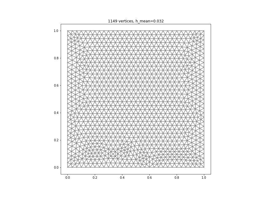
The simulations are performed using FEniCS [2], with a Crank-Nicolson scheme in time [1]. The time step is chosen small enough according to , in order to ensure that the error is driven by the mesh size and not the time step111This is not a kind of CFL condition due to the PFEM, but a matter of space discretization analysis. We only have access to the total error in . Taking a sufficiently small time step allows for the analysis of this error as a function of , to be able to observe the order . Note in particular that Crank-Nicolson scheme is unconditionality stable and symplectic. . These tests have been run on a personal computer (Intel Core I7 processor, 24GB of RAM).
![[Uncaptioned image]](/html/2006.15032/assets/Figures/CVoptimal1.png)
| -0.5 | -0.5 | -0.5 | -0.5 | -0.5 | -0.5 | -0.5 | -0.5 | -0.5 | -0.5 | -0.5 | -0.5 | -0.5 | |
| 0.98 | 0.99 | 0.98 | 0.98 | 0.99 | 0.99 | 0.98 | 0.99 | 0.98 | 0.98 | 0.98 | 0.98 | 0.98 | |
| -0.0 | 0.99 | 0.99 | 0.99 | 1.0 | 0.99 | 0.99 | 1.0 | 0.99 | 0.99 | 0.99 | 0.99 | 0.99 | |
| -0.0 | 1.01 | 0.99 | 0.99 | 0.53 | 0.45 | 0.99 | 0.98 | 0.99 | 0.99 | 0.98 | 0.99 | 0.99 |
![[Uncaptioned image]](/html/2006.15032/assets/Figures/CVoptimal2.png)
| -0.5 | -0.5 | -0.5 | -0.5 | -0.5 | -0.5 | -0.5 | -0.5 | -0.5 | -0.5 | -0.5 | -0.5 | -0.5 | |
| 0.99 | 0.99 | 0.97 | 0.95 | 1.75 | 1.45 | 0.96 | 1.51 | 1.04 | 0.96 | 1.01 | 1.02 | 0.96 | |
| 0.0 | 1.97 | 2.03 | 2.03 | 1.45 | 2.03 | 2.03 | 1.49 | 2.03 | 2.03 | 1.02 | 2.02 | 2.03 | |
| 0.02 | 1.5 | 2.03 | 2.03 | 0.94 | 2.03 | 2.03 | 0.97 | 2.02 | 2.03 | 0.57 | 2.02 | 2.03 |
![[Uncaptioned image]](/html/2006.15032/assets/Figures/CVoptimal3.png)
| -0.5 | -0.5 | -0.5 | -0.5 | -0.5 | -0.5 | -0.5 | -0.5 | -0.5 | -0.5 | -0.5 | -0.5 | -0.5 | |
| 0.98 | 0.96 | 0.96 | 0.94 | 1.79 | 1.44 | 0.95 | 1.48 | 1.03 | 0.95 | 1.01 | 1.02 | 0.95 | |
| 0.0 | 1.97 | 1.93 | 1.91 | 1.45 | 1.85 | 1.87 | 1.47 | 1.88 | 1.88 | 1.02 | 1.83 | 1.88 | |
| 0.02 | 1.5 | 3.01 | 2.97 | 0.95 | 1.95 | 3.43 | 0.98 | 1.93 | 3.26 | 0.57 | 1.51 | 3.08 |
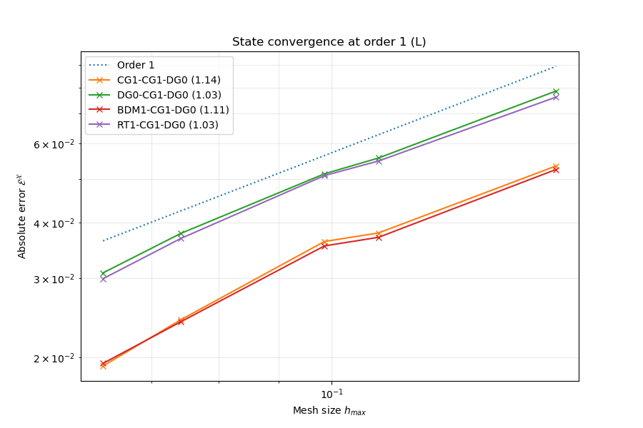
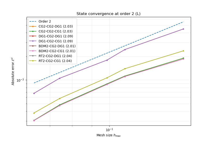
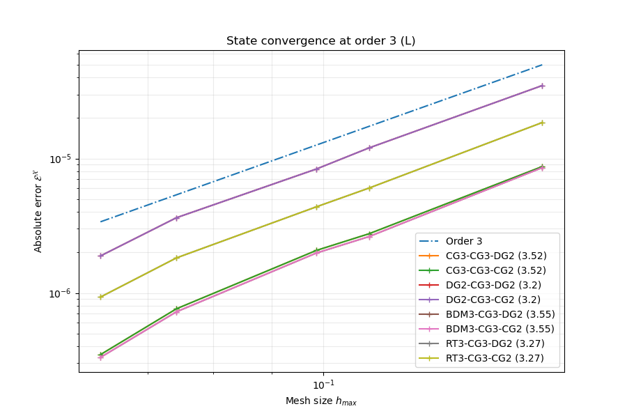
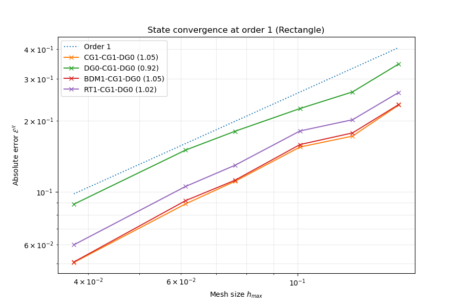
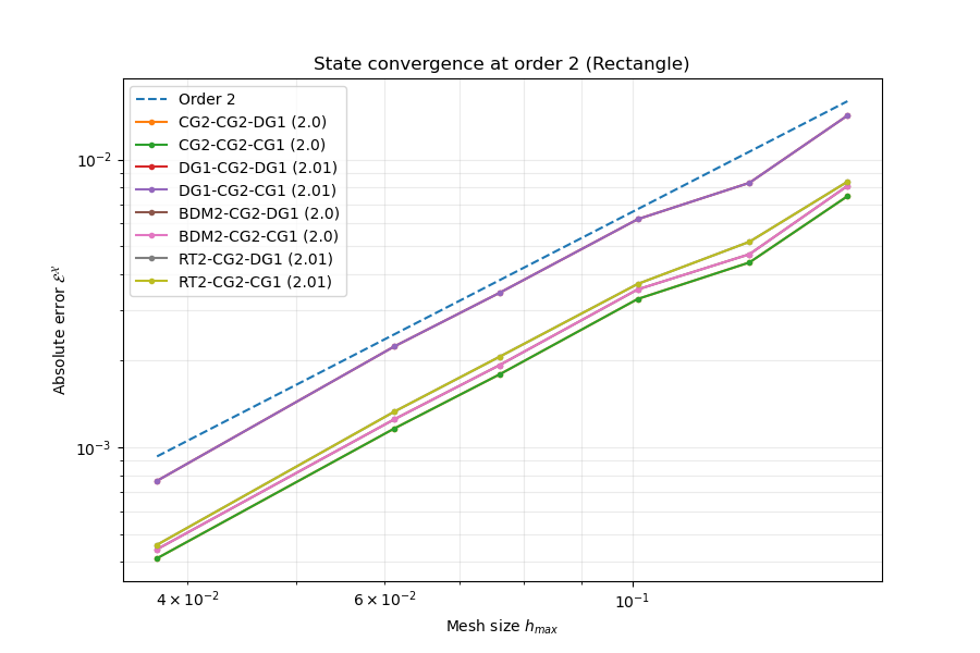
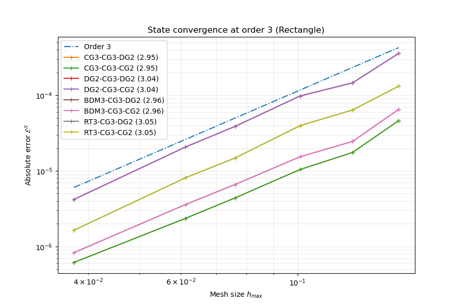
All the convergence rates are presented on Tables 1-2-3 for the absolute error . The associated figures show the convergence rates proven in Theorem 4.2 and Proposition 5.2 for the optimal choices of finite element families among all our tests.
In Theorem 4.2, is assumed to be -conforming. Looking at Tables 1-2-3, this seems indeed necessary to ensure convergence. In every test cases, the rate is negative when is given by discontinuous Galerkin finte elements, no matter the order (we gather lines for , since they give the same results). It has to be noted that assumption (17) is not satisfied in these cases: Theorem 4.2 does not apply.
6.3 About the convergence rate of the Hamiltonian error
So far, compatibility conditions have not been taken into account between , and . In other words, only conforming assumptions have been made, and optimal rates have then been deduced. However, pHs are strongly structured, and in particular, the de Rham cohomology should be respected to improve the efficiency of the PFEM. As a motivation, it is remarkable on Tables 4–5–6 that does not converge at the same rate as , as stated in Corollary 4.3, but at twice its order in a various number of cases.
| -1.0 | -1.0 | -1.0 | -1.0 | -1.0 | -1.0 | -1.0 | -1.0 | -1.0 | -1.0 | -1.0 | -1.0 | -1.0 | |
| 0.83 | 0.8 | 0.81 | 0.8 | 0.8 | 0.81 | 0.8 | 0.81 | 0.81 | 0.8 | 0.82 | 0.81 | 0.8 | |
| -0.1 | 0.81 | 0.82 | 0.81 | 0.66 | 0.82 | 0.81 | 0.81 | 0.82 | 0.81 | 0.83 | 0.82 | 0.81 | |
| -0.1 | 0.8 | 0.81 | 0.81 | 1.09 | 0.99 | 0.81 | 0.82 | 0.81 | 0.81 | 0.84 | 0.81 | 0.81 |
On Table 4, one can see that the Hamiltonian convergence rates when boundary functions are approximated by Discontinuous Galerkin finite elements of order 0, , never reach order , i.e. twice the optimal convergence rate of the state error according to Theorem 5.1. This leads us to conclude that compatibility conditions of Theorem 4.4 are never met for the combinations of finite elements presented on Table 4.
On the contrary, increasing by one order the approximation for boundary terms, both for Discontinuous and Continuous Galerkin and , leads to an order in most cases, as seen on Table 5. Those corresponding to a convergence rate of order for the state error in Table 2 might indeed satisfy the compatibility condition of Theorem 4.4.
| -1.0 | -1.0 | -1.0 | -1.0 | -1.0 | -1.0 | -1.0 | -1.0 | -1.0 | -1.0 | -1.0 | -1.0 | -1.0 | |
| 2.05 | 1.99 | 2.07 | 2.07 | 1.96 | 2.08 | 2.07 | 2.04 | 2.08 | 2.07 | 2.09 | 2.08 | 2.07 | |
| 0.01 | 1.95 | 2.02 | 2.02 | 1.96 | 2.02 | 2.02 | 2.06 | 2.02 | 2.02 | 2.04 | 2.02 | 2.02 | |
| 0.04 | 1.99 | 2.02 | 2.02 | 2.11 | 2.02 | 2.03 | 2.0 | 2.02 | 2.02 | 1.14 | 2.02 | 2.03 |
Analogously, increasing again the approximation at the boundary, i.e. taking or finite elements, allows for a Hamiltonian convergence rate reaching order 4, inviting us to conjecture that compatibility conditions of Theorem 4.4 are met for boldface convergence rate of Table 6. Remark that we do not have a sufficiently small time step to be able to numerically observe order 6, if any.
| -1.0 | -1.0 | -1.0 | -1.0 | -1.0 | -1.0 | -1.0 | -1.0 | -1.0 | -1.0 | -1.0 | -1.0 | -1.0 | |
| 1.99 | 1.95 | 1.93 | 1.93 | 1.95 | 1.93 | 1.93 | 1.96 | 1.91 | 1.93 | 2.0 | 1.91 | 1.93 | |
| 0.01 | 1.95 | 1.88 | 3.94 | 1.95 | 1.98 | 3.92 | 1.95 | 1.77 | 3.91 | 2.04 | 1.94 | 3.93 | |
| 0.04 | 1.95 | — | 4.12 | 1.95 | 4.04 | — | 1.95 | 4.11 | — | 1.14 | 1.94 | — |
To conclude, as pHs deal with a Hamiltonian functional, which can be seen as the primary object, the structure-preserving discretization should mean that has to be accurately discretized for both the power balance (PFEM) and the value of in (compatibility conditions). Together, the PFEM and the compatibility conditions seem to achieve this, making use of the Finite Element Method only. They give the maximal precision with the minimal number of degrees of freedom. Furthermore, the number of degrees of freedom at the boundary being very low in comparison to those of - and -type, it clearly appears that the choice of boundary finite elements proves crucial to reach the expected convergence rates with respect to the finite elements chosen within the domain (as an example, compare the rate obtained with the discretization for and on Table 5 with the same on Table 6).
6.4 More test cases
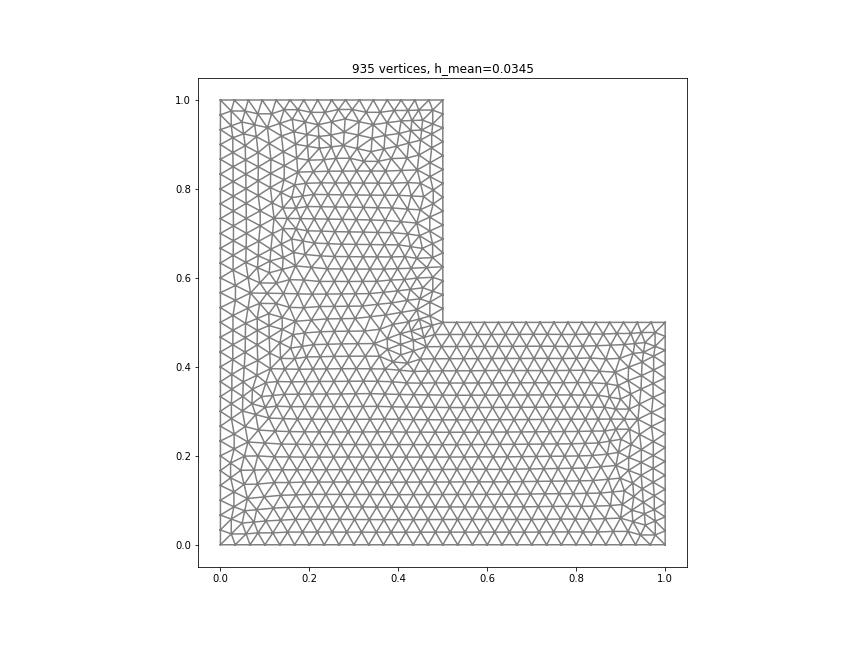
6.4.1 A non-convex case: the -shaped domain
In this section, we test a non-convex case, with an analytical solution given as in the previous tests (boundary control is again given by the restriction of the analytical solution to ), with a time step . One can appreciate on Figure 1 how our results remain valid even for this more complicated domain.
6.4.2 An anisotropic case
As Theorems 4.2 and 4.4 are given for general heterogeneous anisotropic wave equations, a test case for constant anisotropy on the square is consider, with a time step . Let
An analytical solution is then given by: . More precisely
Convergence rates for optimal combinations of finite elements are given on Figure 2.
6.5 Absorbing boundary condition
It can be difficult to deal with dissipative boundary conditions for PDEs. For instance in the port-Hamiltonian formalism, at the continuous level, the dissipation does not appear as a positive bounded operator in the dynamics in general. This means that the dynamics of the port-Hamiltonian systems is not necessarily governed by an operator of the form (even with a lot of work involving lifting operators to fit this formulation, will not be a bounded operator). In other words, the dissipativity is hidden in the domain of the unbounded operator . However, it is expected to recover a finite-dimensional pHs driven by a matrix of the form at the discrete level.
PFEM provides a very easy and convenient way to describe this positive matrix when dealing with admittance or impedance boundary conditions, i.e. absorbing boundary condition in the PDE terminology. The strategy relies on the use of a suitable output feedback law on the finite-dimensional pHs obtained by PFEM in the previous sections (see [48, 47] where this original strategy has been first proposed and explained in full details). Furthermore, this construction gives a well-understood structure to the matrix , which turns out to be of low rank: at most the dimension of as expected, since the damping is applied at the boundary only.
6.5.1 Discretization
More precisely, the following boundary condition is considered, instead of (2), for the admittance boundary condition
| (2Y) |
and the following one instead of (2), for the impedance boundary condition
| (2Z) |
where both the admittance and the impedance are positive and belong to and or are the external inputs.
Remark 6.1.
It is clear that (2Y) and (2Z) generalize (2) and (2S) respectively. Nevertheless, as mentioned above, PFEM does not apply straightforwardly in these more general cases (think about the use of Green’s formula (4) at the beginning of the strategy). The proposed alternative to construct the finite-dimensional dissipative pHs using an output feedback laws seems an elegant way to achieve our goal.
It is easy to write the following relations: between , and (the new control) from (2) and (2Y)
or between , and (the new control) from (2S) and (2Z)
| (34) |
Using a weak formulation, these equalities read in matrix form
or
respectively, where
or
As presented in [47, Remark 2.], this procedure indeed gives rise to finite-dimensional Dirac structures, introducing extra resistive ports, and leading to a pHDAE.
6.5.2 Simulation results
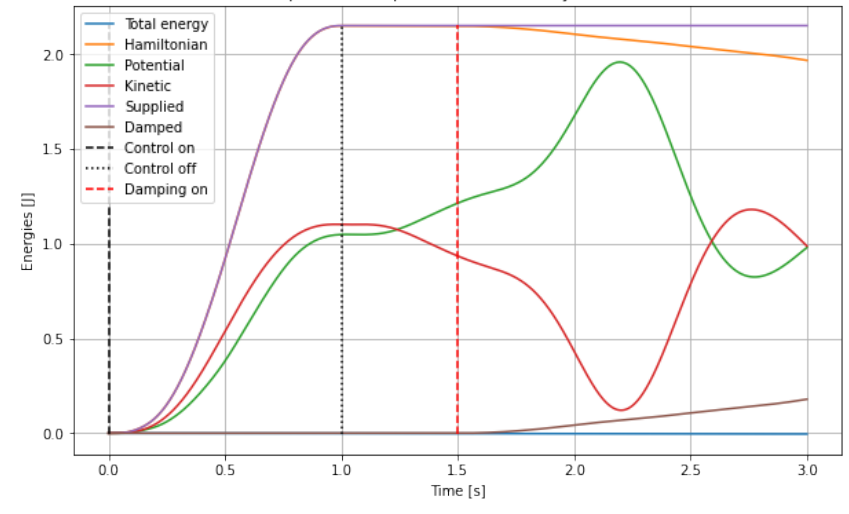
As a worked-out example, let us consider a fully heterogeneous and anisotropic case, with boundary control and boundary damping. The aim is to illustrate how the structure-preserving scheme can be appreciate on the Hamiltonian behaviour and the different kind of energies present in the system (potential, kinetic, supplied and damped).
Let us consider each part of the energy and their sum. The preservation of the physical meaning supposes that the exchanges of energy (e.g. potential to kinetic and vice-versa, boundary-supplied/taken energy to the system and damped into internal energy) must result in the preservation of the first principle of thermodynamics: the sum of all energies must be constant over time. More precisely, let us define the potential energy
the kinetic energy
the boundary-supplied energy
and the damped energy
The total energy present in the system over time is then decomposed as
and the first principle of thermodynamics implies that for all .
For our example on , the non-uniform anisotropic elasticity tensor and the non-uniform heterogeneous mass density are taken as follows
The boundary control is chosen as
while the admittance is defined by
The simulation is performed on the time interval with a time step . The spatial discretization is . The time solver is Assimulo (IDA SUNDIALS) [4]. The integration in time to compute and are done using the midpoint rule. We can appreciate on Figure 3 how the total energy remains constant over time, as physically expected, thanks to the PFEM.
7 Conclusion and perspectives
In this work, the numerical analysis of the Partitioned Finite Element Method applied to the anisotropic and heterogeneous boundary-controlled-and-observed -dimensional wave equation has been carried out. This recent structure-preserving method [12, 13] allows the direct construction of a finite-dimensional port-Hamiltonian system, the underlying Dirac structure of which mimicks the infinite-dimensional Stokes-Dirac structure. This property allows a very accurate discretization of the power balance satisfied by the system. Furthermore, it has been shown that under compatibility conditions resembling those allowing for discrete de Rham complexes, the discrete Hamiltonian converges very fastly toward the continuous one, strengthening the interest of the PFEM, since the versatility of port-Hamiltonian systems aims precisely at modelling the exchange of energies between sub-systems. As an illustration of our main theorems, we have performed 2D simulations on a case where an analytical solution is known, with a non-homogeneous boundary condition: the boundary control, for both convex and non-convex domain. A wide range of usual finite element have been tested. Moreover, impedance-like boundary damping have been carried out to illustrate the structure-preserving property of the PFEM [48, 47].
Several questions remain open, the first one being the case of mixed boundary conditions. Two approaches have been proposed in [11]: a domain decomposition followed by a gyrator interconnection between the two sub-systems, and the use of Lagrange multipliers. The former has the great advantage of remaining an ODE, while the latter transforms into a Differential Algebraic Equation (DAE). The numerical analysis of both alternatives will require deeper investigation.
A second interesting question is the problem of symplectic integration of pHDAE, which naturally arises in various situations such as the aforementioned mixed boundary conditions, or for the heat equation [45, 46]. A scheme has been recently proposed in [40] for this purpose.
Finally, in assumption (7) allowing for regular solutions, is assumed to be a Hilbert space. It is clear that this requires some regularity assumptions on the physical parameters. An interesting future work would be to design a structure-preserving scheme when the physical parameters and are no more regular, e.g. using mollifying methods: refining the constants in the estimates as function of those parameters, as done in this work, seems to be a first step in order to tackle this problem.
References
- [1] S. Abhyankar, J. Brown, E. M. Constantinescu, D. Ghosh, B. F. Smith, and H. Zhang, PETSc/TS: A modern scalable ODE/DAE solver library, tech. rep., 2018.
- [2] M. S. Alnæs, J. Blechta, J. Hake, A. Johansson, B. Kehlet, A. Logg, C. Richardson, J. Ring, M. E. Rognes, and G. N. Wells, The FEniCS Project Version 1.5, Archive of Numerical Software, 3 (2015).
- [3] R. Altmann, V. Mehrmann, and B. Unger, Port-Hamiltonian formulations of poroelastic network models, Mathematical and Computer Modelling of Dynamical Systems, 27 (2021), pp. 429–452.
- [4] C. Andersson, C. Führer, and J. Åkesson, Assimulo: A unified framework for ODE solvers, Mathematics and Computers in Simulation, 116 (2015), pp. 26–43.
- [5] D. N. Arnold, R. S. Falk, and R. Winther, Finite element exterior calculus, homological techniques, and applications, Acta Numerica, 15 (2006), pp. 1–155.
- [6] , Finite element exterior calculus: from Hodge theory to numerical stability, American Mathematical Society. Bulletin. New Series, 47 (2010), pp. 281–354.
- [7] E. Bécache, P. Joly, and C. Tsogka, An Analysis of New Mixed Finite Elements for the Approximation of Wave Propagation Problems, SIAM Journal on Numerical Analysis, 37 (2000), pp. 1053–1084.
- [8] , A New Family of Mixed Finite Elements for the Linear Elastodynamic Problem, SIAM Journal on Numerical Analysis, 39 (2002), pp. 2109–2132.
- [9] P. B. Bochev and J. M. Hyman, Principles of Mimetic Discretizations of Differential Operators, in Compatible Spatial Discretizations, vol. 142 of The IMA Volumes in Mathematics and its Applications, Springer, New York, 2006, pp. 89–119.
- [10] D. Boffi, F. Brezzi, and M. Fortin, Mixed Finite Element Methods and Applications, vol. 44 of Springer Series in Computational Mathematics, Springer, Berlin Heidelberg, 2013.
- [11] A. Brugnoli, F. L. Cardoso-Ribeiro, G. Haine, and P. Kotyczka, Partitioned Finite Element Method for Power-Preserving Structured Discretization with Mixed Boundary Conditions, in 21st IFAC World Congress, vol. 53, Berlin, Germany, July 2020, IFAC, pp. 7647–7652. (invited session).
- [12] F. L. Cardoso-Ribeiro, D. Matignon, and L. Lefèvre, A structure-preserving Partitioned Finite Element Method for the 2D wave equation, IFAC-PapersOnLine, 51 (2018), pp. 119–124. 6th IFAC Workshop on Lagrangian and Hamiltonian Methods for Nonlinear Control LHMNC 2018.
- [13] F. L. Cardoso-Ribeiro, D. Matignon, and L. Lefèvre, A partitioned finite element method for power-preserving discretization of open systems of conservation laws, IMA Journal of Mathematical Control and Information, 38 (2021), pp. 493–533.
- [14] F. L. Cardoso-Ribeiro, D. Matignon, and V. Pommier-Budinger, Port-Hamiltonian model of two-dimensional shallow water equations in moving containers, IMA Journal of Mathematical Control and Information, 37 (2020), pp. 1348–1366.
- [15] J. Cervera, A. J. van der Schaft, and A. Baños, Interconnection of port-Hamiltonian systems and composition of Dirac structures, Automatica, 43 (2007), pp. 212–225.
- [16] M. Cessenat, Mathematical methods in electromagnetism, vol. 41 of Series on Advances in Mathematics for Applied Sciences, World Scientific Publishing Co. Inc., River Edge, NJ, 1996. Linear theory and applications.
- [17] V. Duindam, A. Macchelli, S. Stramigioli, and H. Bruyninckx, Modeling and Control of Complex Physical Systems: The Port-Hamiltonian Approach, Springer-Verlag, Berlin Heidelberg, 2009.
- [18] H. Egger, Structure preserving approximation of dissipative evolution problems, Numerische Mathematik, 143 (2019), pp. 85–106.
- [19] H. Egger, T. Kugler, B. Liljegren-Sailer, N. Marheineke, and V. Mehrmann, On Structure-Preserving Model Reduction for Damped Wave Propagation in Transport Networks, SIAM Journal on Scientific Computing, 40 (2018), pp. A331–A365.
- [20] O. Farle, R.-B. Baltes, and R. Dyczij-Edlinger, A Port-Hamiltonian Finite-Element Formulation for the Transmission Line, in 21st International Symposium on Mathematical Theory of Networks and Systems (MTNS), Groningen, The Netherlands, July 2014, MTNS, pp. 724–728.
- [21] O. Farle, D. Klis, M. Jochum, O. Floch, and R. Dyczij-Edlinger, A port-Hamiltonian finite-element formulation for the Maxwell equations, in 2013 International Conference on Electromagnetics in Advanced Applications (ICEAA), Torino, Italy, September 2013, IEEE, pp. 324–327.
- [22] Y. Feng, Y. Liu, R. Wang, and S. Zhang, A conforming discontinuous Galerkin finite element method on rectangular partitions, Electronic Research Archive, 29 (2021), pp. 2375–2389.
- [23] C. Foiaş and R. M. Temam, Remarques sur les équations de Navier-Stokes stationnaires et les phénomènes successifs de bifurcation, Annali della Scuola Normale Superiore di Pisa. Classe di Scienze. Serie IV, 5 (1978), pp. 28–63.
- [24] G. N. Gatica, A Simple Introduction to the Mixed Finite Element Method: Theory and Applications, SpringerBriefs in Mathematics, Springer, Cham, 2014.
- [25] M. Gerritsma, J. Kunnen, and B. de Heij, Discrete Lie derivative, in Lecture Notes in Computational Science and Engineering, vol. 112 of Lecture Notes in Computational Science and Engineering, Springer, Cham, 2016, pp. 635–643.
- [26] M. Gerritsma, A. Palha, V. Jain, and Y. Zhang, Mimetic Spectral Element Method for Anisotropic Diffusion, in Numerical Methods for PDEs, vol. 15 of SEMA SIMAI Springer Series, Springer, Cham, 2018, pp. 31–74.
- [27] V. Girault and P.-A. Raviart, Finite Element Methods for Navier-Stokes Equations, vol. 5 of Springer Series in Computational Mathematics, Springer, Berlin Heidelberg, 1986.
- [28] S. Gugercin, R. V. Polyuga, C. Beattie, and A. J. van der Schaft, Structure-preserving tangential interpolation for model reduction of port-Hamiltonian systems, Automatica, 48 (2012), pp. 1963–1974.
- [29] G. Haine and D. Matignon, Structure-Preserving Discretization of a Coupled Heat-Wave System, as Interconnected Port-Hamiltonian Systems, in Geometric Science of Information, Nielsen, Frank and Barbaresco, Frédéric, eds., vol. 12829 of Lecture Notes in Computer Science, Springer, Cham, 2021, pp. 191–199.
- [30] G. Haine, D. Matignon, and F. Monteghetti, Long-time behavior of a coupled heat-wave system using a structure-preserving finite element method, Mathematical Reports, 24(74) (2022), pp. 187–215.
- [31] R. R. Hiemstra, D. Toshniwal, R. H. M. Huijsmans, and M. Gerritsma, High order geometric methods with exact conservation properties, Journal of Computational Physics, 257 (2014), pp. 1444–1471.
- [32] R. Hiptmair, Discrete Hodge operators, Numerische Mathematik, 90 (2001), pp. 265–289.
- [33] P. Joly, Variational Methods for Time-Dependent Wave Propagation Problems, in Topics in Computational Wave Propagation: Direct and Inverse Problems, M. Ainsworth, P. Davies, D. Duncan, B. Rynne, and P. Martin, eds., vol. 31 of Lecture Notes in Computational Science and Engineering, Springer, Berlin, Heidelberg, 2003, pp. 201–264.
- [34] P. Kotyczka, Numerical Methods for Distributed Parameter Port-Hamiltonian Systems, TUM.University Press, Munich, 2019. Habilitation.
- [35] P. Kotyczka, B. Maschke, and L. Lefèvre, Weak form of Stokes–Dirac structures and geometric discretization of port-Hamiltonian systems, Journal of Computational Physics, 361 (2018), pp. 442–476.
- [36] M. Kurula and H. Zwart, Linear wave systems on n-D spatial domains, International Journal of Control, 88 (2015), pp. 1063–1077.
- [37] M. Kurula, H. Zwart, A. J. van der Schaft, and J. Behrndt, Dirac structures and their composition on Hilbert spaces, Journal of Mathematical Analysis and Applications, 372 (2010), pp. 402–422.
- [38] D. Lee, A. Palha, and M. Gerritsma, Discrete conservation properties for shallow water flows using mixed mimetic spectral elements, Journal of Computational Physics, 357 (2018), pp. 282–304.
- [39] F. Lepe, D. Mora, and R. Rodríguez, Locking-free finite element method for a bending moment formulation of Timoshenko beams, Computers & Mathematics with Applications, 68 (2014), pp. 118–131.
- [40] V. Mehrmann and R. Morandin, Structure-Preserving Discretization for Port-Hamiltonian Descriptor Systems, in IEEE 58th Conference on Decision and Control (CDC), Nice, France, 2019, IEEE, pp. 6863–6868.
- [41] P. Monk, Finite element methods for Maxwell’s equations, Numerical Mathematics and Scientific Computation, Oxford University Press, New York, 2003.
- [42] T. Oliveira and A. Portela, Weak-form collocation – A local meshless method in linear elasticity, Engineering Analysis with Boundary Elements, 73 (2016), pp. 144–160.
- [43] R. Rashad, F. Califano, A. J. van der Schaft, and S. Stramigioli, Twenty years of distributed port-Hamiltonian systems: a literature review, IMA Journal of Mathematical Control and Information, 37 (2020), pp. 1400–1422.
- [44] F.-J. Sayas, Aubin-nitsche estimates are equivalent to compact embeddings, BIT Numerical Mathematics, 44 (2004), pp. 287–290.
- [45] A. Serhani, G. Haine, and D. Matignon, Anisotropic heterogeneous -D heat equation with boundary control and observation: I. Modeling as port-Hamiltonian system, IFAC-PapersOnLine, 52 (2019), pp. 51–56. 3rd IFAC Workshop on Thermodynamic Foundations for a Mathematical Systems (TFMST).
- [46] , Anisotropic heterogeneous -D heat equation with boundary control and observation: II. Structure-preserving discretization, IFAC-PapersOnLine, 52 (2019), pp. 57–62. 3rd IFAC Workshop on Thermodynamic Foundations for a Mathematical Systems (TFMST).
- [47] A. Serhani, D. Matignon, and G. Haine, A Partitioned Finite Element Method for the Structure-Preserving Discretization of Damped Infinite-Dimensional Port-Hamiltonian Systems with Boundary Control, in Geometric Science of Information, Nielsen, Frank and Barbaresco, Frédéric, eds., vol. 11712 of Lecture Notes in Computer Science, Springer, Cham, 2019, pp. 549–558.
- [48] , Partitioned Finite Element Method for port-Hamiltonian systems with Boundary Damping: Anisotropic Heterogeneous 2-D wave equations, IFAC-PapersOnLine, 52 (2019), pp. 96–101. 3rd IFAC Workshop on Control of Systems Governed by Partial Differential Equations (CPDE).
- [49] M. Seslija, J. M. Scherpen, and A. J. van der Schaft, Explicit simplicial discretization of distributed-parameter port-Hamiltonian systems, Automatica, 50 (2014), pp. 369–377.
- [50] J. Toledo, Y. Wu, H. Ramírez, and Y. Le Gorrec, Observer-based boundary control of distributed port-Hamiltonian systems, Automatica, 120 (2020), pp. 109–130.
- [51] V. Trenchant, H. Ramirez, Y. Le Gorrec, and P. Kotyczka, Finite differences on staggered grids preserving the port-Hamiltonian structure with application to an acoustic duct, Journal of Computational Physics, 373 (2018), pp. 673–697.
- [52] M. Tucsnak and G. Weiss, Observation and control for operator semigroups, Birkhäuser Advanced Texts: Basler Lehrbücher, Birkhäuser Verlag, Basel, 2009.
- [53] A. van der Schaft and D. Jeltsema, Port-Hamiltonian Systems Theory: An Introductory Overview, Foundations and Trends® in Systems and Control, 1 (2014), pp. 173–378.
- [54] A. J. van der Schaft and B. Maschke, Hamiltonian formulation of distributed-parameter systems with boundary energy flow, Journal of Geometry and Physics, 42 (2002), pp. 166–194.
- [55] N. M. T. Vu, L. Lefèvre, and B. Maschke, A structured control model for the thermo-magneto-hydrodynamics of plasmas in tokamaks, Mathematical and Computer Modelling of Dynamical Systems, 22 (2016), pp. 181–206.
Appendix A Technical lemmas
The following lemma gives an upper bound for in (18), namely from (H4), although not optimal for general geometry (e.g. for convex domains).
Lemma A.1.
Proof.
We provide here the two technical lemmas used in the proof of Theorem 4.2.
Lemma A.2.
Under the assumptions of Theorem 4.2, one has
Proof.
Lemma A.3.
Under the assumptions of Theorem 4.2, one has for all
Proof.
Writing
the first term on the right-hand side is bounded thanks to (18), with ,
and by (17), still with ,
Since , hypothesis (H4) gives
Let us focus now on to conclude. Since is a projector from onto , one has . Hence
where we have used the lower bound for from the first to the second line. From the second to the third line, we have used the norm of the projector , which is 1 thanks to its orthogonality in endowed with the inner product , for all . Finally, we have used the upper bound for from the third to the fourth line.