Differential Privacy of Hierarchical Census Data:
An Optimization Approach

Abstract

This paper is motivated by applications of a Census Bureau interested in releasing aggregate socio-economic data about a large population without revealing sensitive information about any individual. The released information can be the number of individuals living alone, the number of cars they own, or their salary brackets. Recent events have identified some of the privacy challenges faced by these organizations [5]. To address them, this paper presents a novel differential-privacy mechanism for releasing hierarchical counts of individuals. The counts are reported at multiple granularities (e.g., the national, state, and county levels) and must be consistent across all levels. The core of the mechanism is an optimization model that redistributes the noise introduced to achieve differential privacy in order to meet the consistency constraints between the hierarchical levels. The key technical contribution of the paper shows that this optimization problem can be solved in polynomial time by exploiting the structure of its cost functions. Experimental results on very large, real datasets show that the proposed mechanism provides improvements of up to two orders of magnitude in terms of computational efficiency and accuracy with respect to other state-of-the-art techniques.

1 Introduction

The release of datasets containing sensitive information about a large number of individuals is central to a number of statistical analysis and machine learning tasks. For instance, the US Census Bureau publishes socio-economic information about individuals, which is then used as input to train classifiers or predictors, release important statistics about the US population, and take decisions relative to elections and financial aid. roles of a Census Bureau is to report group size queries, which are especially useful to study the skewness of a distribution. For instance, in 2010, the US Census Bureau released 33 datasets of such queries [30]. Group size queries partition a dataset in groups and evaluate the size of each group. For instance, a group may be the households that are families of four members, or the households owning three cars.

The challenge is to release these datasets without disclosing sensitive information about any individual in the dataset. The confidentiality of information in the decennial census is also required by law. Various techniques for limiting a-priori the disclosed information have been investigated in the past, including anonymization [28] and aggregations [31]. However, these techniques have been consistently shown ineffective in protecting sensitive data [18, 28], For instance, the US Census Bureau confirmed [2] that the disclosure limitations used for the 2000 and 2010 censuses had serious vulnerabilities which were exposed by the Dinur and Nissim’s reconstruction attack [9]. Additionally, the 2010 Census group sizes were truncated due to the lack of privacy methods for protecting these particular groups [4].

This paper addresses these limitations through the framework of Differential Privacy [10], a formal approach to guarantee data privacy by bounding the disclosure risk of any individual participating in a dataset. Differential privacy is considered the de-facto standard for privacy protection and has been adopted by various corporations [12, 29] and governmental agencies [1]. Importantly, the 2020 US Census will use an approach to disclosure avoidance that satisfies the notion of Differential Privacy [5].

Differential privacy works by injecting carefully calibrated noise to the data before release. However, whereas this process guarantees privacy, it also affects the fidelity of the released data. In particular, the injected noise often produces datasets that violate consistency constraints of the application domain. In particular, group size queries must be consistent in a geographical hierarchy, e.g., the national, state, and county levels. Unfortunately, the traditional injection of independent noise to the group sizes cannot ensure the consistency of hierarchical constraints.

To overcome this limitation, this paper casts the problem of privately releasing group size data as a constraint optimization problem that ensures consistency of the hierarchical dependencies. However, the optimization problem that redistributes noise optimally is intractable for real datasets involving hundreds of millions of individuals. In fact, even its convex relaxation, which does not guarantee consistency, is challenging computationally. This paper addresses these challenges by proposing mechanisms based on a dynamic programming scheme that leverages both the hierarchical nature of the problem and the structure of the objective function.

Notation	Description
$\mathcal{P}$	The set of all users
$\mathcal{U}$	The set of all units (e.g., home addresses)
$\mathcal{R}$	The set of all regions (e.g., census blocks, states)
$\mathcal{Z}$	The set of all unit quantities (e.g., the number of cars a user owns)
$\mathcal{S}$	The set of all group sizes
$\mathcal{T}$	The region hierarchy
$\mathcal{R}_{\ell}$	The set of regions in level $\ell$ of $\mathcal{T}$
$L$	The number of levels in $\mathcal{T}$
$N$	The number of group sizes, i.e., $|\mathcal{S}|$
$G$	The total count of groups, i.e., $\sum_{r\in R_{\ell}}\sum_{i=1}^{N}n^{r}_{i}$ for any $\ell\in[L]$
$n$	The number of individuals in the dataset
$n_{s}^{r}$	The number of groups of size $s$ in region $r$
$\bm{n}^{r}$	The vector of group sizes for region $r$
$a_{s}^{r}$	A node in the DP tree associated to region $r$ and group size $s$
$\bm{\tau}_{s}^{r}$	The cost table associated to node $a_{s}^{r}$
$\bm{\tau}_{s}^{r}(v)$	The cost value of $\bm{\tau}_{s}^{r}$ associated to value $v$
$\bm{\phi}_{s}^{r}$	The contribution of $a^{r}_{s}$ children costs tables
$D_{s}^{r}$	The domain associated to node $a_{s}^{r}$
$ch(r)$	The set of children regions of region $r$ in $\mathcal{T}$
$pa(r)$	The parent region of region $r$ in $\mathcal{T}$

Table 1: Important symbols adopted in the paper.

Paper Contributions

The paper focuses on the Privacy-preserving Group Size Release (PGSR) problem for releasing differentially private group sizes that preserves hierarchical consistency. Its contributions are summarized as follows: (1) It proposes several differentially private mechanisms that rely on an optimization approach to release both accurate and consistent group sizes. (2) It shows that the differentially private mechanisms can be implemented in polynomial time, using a dynamic program that exploits the hierarchical nature of group size queries, the structure of the objective functions, and cumulative counts. (3) Finally, it evaluates the mechanisms on very large datasets containing over 300,000,000 individuals. The results demonstrate the effectiveness and scalability of the proposed mechanisms that bring several orders of magnitude improvements over the state of the art.

Paper Organization

The paper is organized as follows. Section 2 introduces the notation and describes the group size release problem. Section 3 reviews the privacy notion adopted in this work, as well as some useful results adopted in the privacy analysis of the proposed mechanisms. Section 4 presents the Privacy-Preserving Group Size Release (PGSR) problem and discusses its privacy, consistency, validity, and faithfulness criteria. Section 5 presents $\mathcal{M}_{H}$, a two-step mechanism for the PGSR problem that uses an optimization-based post-processing step to satisfy the PGSR criteria. Section 6 presents $\mathcal{M}_{H}^{\textsl{dp}}$, an exact mechanism for the PGSR problem that exploits dynamic programming. While the proposed mechanism is exact, it becomes ineffective for very large real-life applications. An efficient polynomial-time solution for solving the dynamic program is presented in Section 7. Section 8 discusses how to use cumulative queries to reduce the amount of noise required to produce the privacy-preserving counts and Section 9 presents $\mathcal{M}_{c}$, a sub-optimal algorithm to solve the PGSR under cumulative queries. Then, Section 9.1 and Section 9.2 present, respectively, an approximate and exact efficient dynamic-programming mechanism for solving the PGSR problem under cumulative queries. Finally, Section 10 discusses related work, Section 11 report an evaluation of the proposed mechanisms on several realistic datasets, and Section 12 concludes the work.

A summary of the important symbols adopted in the paper is provided in Table 1. The appendix contains the proofs for all lemmas and theorems.

2 Problem Specification

This paper is motivated by applications from the US Census Bureau, whose goal is to release socio-demographic features of the population grouped by census blocks, counties, and states. For instance, the bureau is interested in releasing information such as the number of people in a household and how many cars they own. This section provides a generic formalization of this release problem.

Consider a dataset $D=\{(p_{i},u_{i},r_{i},z_{i})\}_{i=1}^{n}$ containing $n$ tuples $(p_{i},u_{i},r_{i},z_{i})\in\mathcal{P}\times\mathcal{U}\times\mathcal{R}\times\mathcal{Z}$ denoting, respectively, a (randomly generated) identifier for user $i\in[n]$, its unit identifier (e.g., the home address where she lives), the region in which she lives, (e.g., a census block), and a unit quantity describing a socio-demographic feature, e.g., the number of cars she owns, or her salary bracket. The set of users sharing the same unit forms a group and $G_{u}=\{p_{i}\in\mathcal{P}\>|\>u_{i}=u\}$ denotes the group of unit $u$. The socio-demographic feature of interest is the sum of the unit quantities of a group $G_{u}$, i.e., $\sigma_{u}=\sum_{p_{i}\in G_{u}}z_{i}$.

user	unit	region	quantity
$01$	A	GA	1
$02$	B	GA	1
$03$	A	GA	1
$04$	A	GA	1
$05$	C	GA	1
$06$	D	NY	1
$07$	E	NY	1
$08$	D	NY	1
$09$	D	NY	1
${10}$	F	NY	1
${11}$	F	NY	1

Table 2: Example dataset describing the user identifier $p_{i}\in\mathcal{P}$, its unit $u_{i}\in\mathcal{U}$, the user’s region $r_{i}\in\mathcal{R}$ and the unit quantity $z_{i}\in\mathcal{Z}$ $(i\in[11])$.

region	$u$	group $G_{u}$	$\sigma_{u}$
GA	A	$\{01,03,04\}$	$3$
	B	$\{02\}$	$1$
	C	$\{05\}$	$1$
NY	D	$\{06,08,09\}$	$3$
	E	$\{07\}$	$1$
	F	$\{10,11\}$	$2$

Table 3: Groups $(G_{u})$ and sum of unit quantities ($\sigma_{u}$) for the users $u\in\mathcal{U}$ of Table 3.

 Example​ 1

Consider the example dataset of Table 3. It shows $11$ users ($p_{i}\in\mathcal{P}$, their addresses (unit identifiers $u_{i}\in\mathcal{U}$) , the US states in which they live (regions $r_{i}\in\mathcal{U}$), and the associated 0/1 quantity denoting a feature of interest ($z_{i}\in\mathcal{Z})$. In the running example, the feature of interest is always 1, since the application is interested with the composition of the household, i.e., how many people live at the same address. Hence the groups identify households and the sums of unit quantities represent household sizes. The set of users, units, and regions, are, respectively: $\mathcal{P}=\{\textsl{01},\ldots,\textsl{11}\}$, $\mathcal{U}=\{A,B,C,D,E,F\}$, and $\mathcal{R}=\{\textsl{GA},\textsl{NY},\textsl{US}\}$. The table shows that some users live in the same address (e.g., user 01, 03, and 04 all live in address $A$), identifying the users of group $G_{A}$, as illustrated in Table 3. In addition to the groups $G_{u}$, for all unit $u\in\mathcal{U}$, Table 3 also reports the sum of unit quantities $\sigma_{u}$ associated with each group $G_{u}$. In the example, these quantities denote the household sizes. For instance, $\sigma_{A}=3$ denotes that 3 users live in unit $A$ (e.g., in group $G_{A}$).

In addition to the dataset, the census bureau works with a region hierarchy that is formalized by a tree $\mathcal{T}$ of $L$ levels. Each level $\ell\in[L]$ is associated with a set of regions $\mathcal{R}_{\ell}\subseteq\mathcal{R}$, forming a partition on $D$. Region $r^{\prime}$ is a subregion of region $r$, which is denoted by $r^{\prime}\prec r$, if $r^{\prime}$ is contained in $r$ and $\text{lev}(r^{\prime})=\text{lev}(r)+1$, where $\text{lev}(r)$ denotes the level of $r$. The root level contains a single region $r^{\top}$. The children of $r$, i.e., $ch(r)=\{r^{\prime}\in\mathcal{R}|r^{\prime}\prec r\}$ is the set of regions that partitions $r$ in the next level of the hierarchy and $pa(r)$ denotes the parent of region $r$ ($r\neq r^{\top}$). Figure 1 provides an illustration of a hierarchy of 2 levels. Each node represents a region. The regions GA and NY form a partition of region US.

The set $\mathcal{S}$ of all unit sizes, ($\{\sigma_{u}\>|\>u\in\mathcal{U}\}\subseteq\mathcal{S}$), also plays an important role. Indeed, the bureau is interested in releasing, for every unit size $\sigma\in\mathcal{S}$, the quantity $n_{\sigma}=|\{G_{u}\>|\>u\in\mathcal{U},\sigma_{u}=\sigma\}|$, i.e., the number of groups of size $\sigma$. The number of groups with size $\sigma\in\mathcal{S}$ and region $r\in\mathcal{R}$ is denoted by $n_{\sigma}^{r}=|\{u\in\mathcal{U}\>|\>\sigma_{u}=\sigma\land u\in r\}|$ and $\bm{n}^{r}=(n_{1}^{r},\ldots,n_{N}^{r})$ denotes the vector of group sizes for region $r$, where $N=|\mathcal{S}|$.

 Example​ 2

In the running example, Figure 1 illustrates a region hierarchy, depicting US as the root region, at level 1 of the hierarchy. Its children $\textsl{ch}(\textsl{US})=\{\textsl{GA},\textsl{NY}\}$ represent the states of Georgia and New York, at level 2 of the hierarchy. Table 4 illustrates the group size table that, for each group size $s\in[N=5]$, counts the number of groups that are households of size $s$. For instance, in region GA, there two groups $u$ whose size $\sigma_{u}=1$: They are groups A and B; in region NY, is a single group whose size is equal $1$: E; Finally, in region US there three groups whose size $\sigma_{u}=1$: A, B, and E (represented in the first row of the table). The group vectors, for each region, are, respectively: $\bm{n}^{\textsl{GA}}=(2,0,1,0,0)$, $\bm{n}^{\textsl{NY}}=(1,1,1,0,0)$, and $\bm{n}^{\textsl{US}}=(3,1,2,0,0)$.

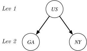
Figure 1: A region hierarchy associated to the example of Table 3.

group sizes	Lev 2		Lev 1
	GA	NY	US
$1$	2	1	3
$2$	0	1	1
$3$	1	1	2
$4$	0	0	0
$5=|\mathcal{S}|=N$	0	0	0
	$\bm{n}^{GA}$	$\bm{n}^{NY}$	$\bm{n}^{US}$

Table 4: The hierarchical group-size quantities associated to the example dataset of Table 3.

It is now possible to define the problem of interest to the bureau: The goal is to release, for every group size $s\in[N]$ and region $r\in\mathcal{R}$, the numbers $n_{s}^{r}$ of groups of size $s$ in region $r$, while preserving individual privacy. The region hierarchy and the group sizes $\mathcal{S}$ are considered public non-sensitive information. The entries associating users with groups (see Table 3) are sensitive information. Therefore, the paper focuses on protecting the privacy of such information. For simplicity, this paper assumes that the region hierarchy has exactly $L$ levels. The paper also focuses on the vastly common case when $z_{i}\in\{0,1\}\ (i\in[n])$, but the results generalize to arbitrary $z_{i}$ values.

3 Differential Privacy

This paper adopts the framework of differential privacy [10, 11], which is the de-facto standard for privacy protection.

 Definition​ 1 (Differential Privacy [10])

A randomized algorithm $\mathcal{M}:{\mathscr{D}}\to{\mathscr{R}}$ is $\epsilon$-differentially private if

$$\Pr[\mathcal{M}(D_{1})\in O]\leq\exp(\epsilon)\Pr[\mathcal{M}(D_{2})\in O],$$ (1)

for any output response $O\subseteq{\mathscr{R}}$ and any two datasets $D_{1},D_{2}\in{\mathscr{D}}$ differing in at most one individual (called neighbors and written $D_{1}\sim D_{2}$).

Parameter $\epsilon>0$ is the privacy loss of the algorithm, with values close to $0$ denoting strong privacy. Intuitively, the definition states that the probability of any event does not change much when a single individual data is added or removed to the dataset, limiting the amount of information that the output reveals about any individual.

This paper relies on the global sensitivity method [10]. The global sensitivity $\Delta_{q}$ of a function $q:{\mathscr{D}}\to\mathbb{R}^{k}$ (also called query) is defined as the maximum amount by which $q$ changes when a single individual is added to, or removed from, a dataset:

$$\Delta_{q}=\max_{D_{1}\sim D_{2}}\|q(D_{1})-q(D_{2})\|_{1}.$$ (2)

Queries in this paper concern the group size vectors $\bm{n}^{r}$ and neighboring datasets differ by the presence or absence of at most one record (see Tables 3 and 4).

The global sensitivity is used to calibrate the amount of noise to add to the query output to achieve differential privacy. There are several sensitivity-based mechanisms [10, 26] and this paper uses the Geometric mechanism [17] for integral queries. It relies on a double-geometric distribution and has slightly less variance than the ubiquitous Laplace mechanism [10].

 Definition​ 2 (Geometric Mechanism [17])

Given a dataset $D$, a query $q:{\mathscr{D}}\to\mathbb{R}^{k}$, and $\epsilon>0$, the geometric mechanism adds independent noise to each dimension of the query output $q(D)$ using the distribution

$$P(X\!=\!v)\!=\!\frac{1-e^{-\epsilon}}{1+e^{-\epsilon}}\,e^{\left(-\epsilon\frac{|v|}{\Delta_{q}}\right)}.$$

This distribution is also referred to as double-geometric with scale $\Delta_{q}/\epsilon$. In the following, $Geom(\lambda)^{k}$ denotes the i.i.d. double-geometric distribution over $k$ dimensions with parameter $\lambda$. The geometric mechanism satisfies $\epsilon$-differential privacy [17]. Differential privacy also satisfies several important properties [11].

 Lemma​ 1 (Sequential Composition)

The composition of two $\epsilon$-differentially private mechanisms ($\mathcal{M}_{1}$, $\mathcal{M}_{2}$) satisfies $2\epsilon$-differential privacy.

 Lemma​ 2 (Parallel Composition)

Let $D_{1}$ and $D_{2}$ be disjoint subsets of $D$ and $\mathcal{M}$ be an $\epsilon$-differential private algorithm. Computing $\mathcal{M}(D\cap D_{1})$ and $\mathcal{M}(D\cap D_{2})$ satisfies $\epsilon$-differential privacy.

 Lemma​ 3 (Post-Processing Immunity)

Let $\mathcal{M}$ be an $\epsilon$-differential private algorithm and $g$ be an arbitrary mapping from the set of possible output sequences $O$ to an arbitrary set. Then, $g\circ\mathcal{M}$ is $\epsilon$-differential private.

4 The Privacy-Preserving Group Size Release Problem

This section formalizes the Privacy-preserving Group Size Release (PGSR) problem [21]. Consider a dataset $D$, a region hierarchy $\mathcal{T}$ for $D$, where each node $a^{r}$ in $\mathcal{T}$ is associated with a vector $\bm{n}^{r}\in\mathbb{Z}_{+}^{N}$ describing the group sizes for region $r\in\mathcal{R}$, and let $G=\sum_{s\in[N]}n^{\top}_{s}$ be the total number of individual groups in $D$, which is public information (see Figure 2 for an example). The PGSR problem consists in releasing a hierarchy of group sizes $\tilde{\mathcal{T}}=\langle\tilde{\bm{n}}^{r}\>|\>r\in\mathcal{R}\rangle$ that satisfies the following conditions:

1. Privacy: $\tilde{\mathcal{T}}$ is $\epsilon$-differentially private.

2. Consistency: For each region $r\in\mathcal{R}$ and group size $s\in\mathcal{S}$, the group sizes in the subregions $r^{\prime}$ of $r$ add up to those in region $r$:

   $$\tilde{n}^{r}_{s}=\sum_{{r^{\prime}}\in ch(r)}\tilde{n}^{r^{\prime}}_{s}.$$

3. Validity: The values $\tilde{n}_{s}^{r}$ are non-negative integers.

4. Faithfulness: The group sizes at each level $\ell$ of the hierarchy add up to the value $G$:

   $$\sum_{r\in\mathcal{R}_{\ell}}\sum_{s\in[N]}\tilde{n}^{r}_{s}=G.$$

These constraints ensure that the hierarchical group size estimates satisfy all publicly known properties of the original data.

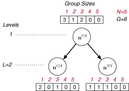
Figure 2: Group size hierarchy $\mathcal{T}_{2}$ associated with the dataset of Table 3.

5 The Direct Optimization-Based PGSR Mechanism

This section presents a two-step mechanism for the PGSR problem, first introduced in [21]. The first step produces a noisy version of the group sizes, whereas the second step restores the feasibility of the PGSR constraints while staying as close as possible to the noisy counts. The first step produces a noisy hierarchy $\tilde{\mathcal{T}}=\{\tilde{\bm{n}}^{r}\>|\>r\in\mathcal{R}\}$ using the geometric mechanism with parameter $\lambda=\frac{2L}{\epsilon}$ on the vectors $\bm{n}^{r}$:

$$\tilde{\bm{n}}^{r}=\bm{n}^{r}+\textsl{Geom}\Big{(}\frac{2L}{\epsilon}\Big{)}^{N}.$$ (3)

The following lemma and theorem, whose proofs are in the appendix, show that this step satisfies $\epsilon$-differential privacy.

 Lemma​ 4

The sensitivity $\Delta_{\bm{n}}$ of the group estimate query is 2.

 Theorem​ 1

$\mathcal{M}_{H}$ satisfies $\epsilon$-differential privacy.

Proofs for all Theorems and Lemmas are reported in the appendix.

The output of the first step satisfies Condition 1 of the PGSR problem but it will violate (with high probability) the other conditions. To restore feasibility, this paper uses a post-processing strategy similar to the one proposed in [13] for mobility applications and in [21]. After generating $\tilde{\mathcal{T}}$ using Equation 3, the mechanism post-processes the values $\tilde{\bm{n}}^{r}$ of $\tilde{\mathcal{T}}$ through the Quadratic Integer Program (QIP) depicted in Model 1. Its goal is to find a new region hierarchy $\hat{\mathcal{T}}$, optimizing over the variables $\hat{\bm{n}}^{r}\!=\!(\hat{n}_{1}^{r}\ldots\hat{n}_{N}^{r})$ for each $r\!\in\!\mathcal{R}$, so that their values stay close to the noisy counts of the first step, while satisfying faithfulness (Constraint (H2)), consistency (Constraint (H3)), and validity (Constraint (H4)). In the optimization model, $D_{s}^{r}$ represents the domain (of integer, non-negative values) of $\hat{n}^{r}_{s}$. The resulting mechanism is called the Hierarchical PGSR and denoted by $\mathcal{M}_{H}$. It satisfies $\epsilon$-differential privacy because of post-processing immunity (Lemma 3), since the post-processing step of $\mathcal{M}_{H}$ uses exclusively differentially private information ($\tilde{\mathcal{T}}$).

Model 1 The $\mathcal{M}_{H}$ post-processing step

$$\operatornamewithlimits{Minimize~{}}_{\left\{\hat{\bm{n}}^{r}\right\}_{r\in\mathcal{R}}}\;\; \sum_{r\in\mathcal{R}}\left|\hat{\bm{n}}^{r}-\tilde{\bm{n}}^{r}\right|_{2}^{2}$$ (H1)

$$\operatornamewithlimits{Subject~{}to:}\;\; \sum_{r\in\mathcal{R}_{\ell}}\sum_{s\in[N]}\hat{n}^{r}_{s}=G \forall\ell\in[L]$$ (H2)

$$\sum_{c\in ch(r)}\hat{n}_{s}^{c}=\hat{n}_{s}^{r}\qquad \forall r\in\mathcal{R},s\in[N]$$ (H3)

$$\hat{n}^{r}_{s}\in D^{r}_{s} \forall r\in\mathcal{R},s\in[N]$$ (H4)

Solving this QIP is intractable for the datasets of interest to the census bureau. Therefore, the experimental results consider a version of $\mathcal{M}_{H}$ that relaxes the integrability constraint (H4) and rounds the solutions. However, the resulting optimization problem becomes convex but presents two limitations: (i) its final solution $\hat{T}$ may violate the PGSR consistency (2) and faithfulness (4) conditions, and (ii) the mechanism is still too slow for very large problems.

6 The Dynamic Programming PGSR Mechanism

To overcome the $\mathcal{M}_{H}$ limitations discussed above, this section proposes a dynamic-programming approach for the post-processing step and its convex relaxation. The resulting mechanism is called the Dynamic Programming PGSR mechanism and denoted by $\mathcal{M}_{H}^{\textsl{dp}}$. The dynamic program relies on a new hierarchy $\mathcal{T}^{\text{dp}}$ that modifies the original region hierarchy $\mathcal{T}$ as follows. It creates as many subtrees as the number $N$ of group sizes $\mathcal{S}$. In each of these subtrees, node $a^{r}_{s}$ is associated with the number $n_{s}^{r}$ of groups of size $s$ in region $r$. Its children $\{a_{s}^{c}\}_{c\in ch(r)}$ are associated with the numbers $n_{s}^{c}$, and so on. Thus, the nodes of subtree $s$ represent the groups of size $s$ for all the regions in $\mathcal{R}$. Finally, the new hierarchy has a root note $a^{\top}$ that represents the total number $G$ of groups: It is associated with a dummy region $\top$ whose children are the root nodes of the $N$ subtrees introduced above. The resulting region hierarchy is denoted $\mathcal{T}^{\textsl{dp}}$.

 Example​ 3

The region hierarchy $\mathcal{T}^{\textsl{dp}}$ associated with the running example is shown in Figure 3. The root node $a^{\top}$ is associated with the total number of groups in $D$, i.e., $G=6$. Its children $a_{1}^{\textsl{US}},\dots,a_{5}^{\textsl{US}}$ represent the group sizes for the root of the region hierarchy for each group size $s\in[N=5]$. Subtree 1, rooted at $a_{1}^{\textsl{US}}$, has two children: $a_{1}^{\textsl{GA}}$ and $a_{1}^{\textsl{NY}}$, representing the number of groups of size $1$: $n_{1}^{\textsl{GA}}$ and $n_{1}^{\textsl{NY}}$. The figure illustrates the association of each node $a_{s}^{r}$ with its real group size $n_{s}^{r}$ (in red) and its noisy group size generated by the geometrical mechanism (in blue and parenthesis).

Note that (i) the value of a node equals to the sum of the values of its children, (ii) the group sizes at a given level add up to $G$, and (iii) the PGSR consistency conditions of the nodes in a subtree are independent of those of other subtrees. These observations allow us to develop a dynamic program that guarantees the PGSR conditions and exploits the independence of each subtree associated with groups of size $s$ to solve the post-processing problem efficiently.

For notational simplicity, the presentation omits the subscripts denoting the group size $s$ and focuses on the computation of a single subtree representing a group of size $s$. The dynamic program associates a cost table $\bm{\tau}^{r}$ with each node $a^{r}$ of $\mathcal{T}^{\textsl{dp}}$. The cost table represents a function $\bm{\tau}^{r}:D^{r}\to\mathbb{R}_{+}$ that maps values (i.e., group sizes) to costs, where $D^{r}$ is the domain (a set of natural numbers) of region $r$. Intuitively, $\bm{\tau}^{r}(v)$ is the optimal cost for the post-processed group sizes in the subtree rooted at $a^{r}$ when its post-processed group size is equal to $v$, i.e., $\hat{n}^{r}=v$. The key insight of the dynamic program is the observation that the optimal cost for $\bm{\tau}^{r}(v)$ can be computed from the cost tables $\bm{\tau}^{c}$ of each of its children $c\in\textsl{ch}(r)$ using the following:

$$\bm{\tau}^{r}(v)= \Big{(}v-\tilde{n}^{r}\Big{)}^{2} +$$ (4a)

$$\hskip 20.0pt\bm{\phi}^{r}(v) =\operatornamewithlimits{Minimize~{}}_{\{x_{c}\}_{c\in\textsl{ch}(r)}} \sum_{c\in\textsl{ch}(r)}\bm{\tau}^{c}(x_{c})$$ (4b)

$$\operatornamewithlimits{Subject~{}to:} \sum_{c\in\textsl{ch}(r)}x_{c}=v$$ (4c)

$$x_{c}\in D^{c}\qquad\forall{c\in\textsl{ch}(r)}.$$ (4d)

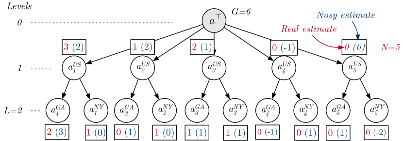
Figure 3: Region hierarchy $\mathcal{T}^{\textsl{dp}}$ associated with the dataset of Table 3.

In the above, (4a) describes the cost for $v$ of deviating from the noisy group size $\tilde{n}^{r}$. The function $\bm{\phi}^{r}(v)$, defined in (4b), (4c), and (4d), uses the cost table of the children of $r$ to find the combination of post-processed group sizes $\{x_{c}\in D^{c}\}_{c\in\textsl{ch}(r)}$ of $r$’s children that is consistent (4c) and minimizes the sum of their costs (4b).

$\bm{v}$	$\tau_{1}^{\textsl{GA}}$	$\tau_{1}^{\textsl{NY}}$	$\tau_{1}^{\textsl{US}}$
$\bm{0}$	$9$	${}^{\star}0$	$4$	$\!+\!\min(9\!+\!0)$
$\bm{1}$	$4$	$1$	$1$	$\!+\!\min(9\!+\!1,4\!+\!0)$
$\bm{2}$	$1$	$4$	$0$	$\!+\!\min(0\!+\!4,4\!+\!1,1\!+\!0)$
$\bm{3}$	${}^{\star}0$	$9$	${}^{\star}1$	$\!+\!\min(0\!+\!0,1\!+\!1,4\!+\!4,9\!+\!9)$
$\bm{4}$	$1$	$16$	$4$	$\!+\!\min(1\!+\!0,0\!+\!1,1\!+\!4,\ldots)$

Table 5: Example of cost table computation for subtree associated to the group 1 estimates.

The dynamic program exploits these concepts in two phases. The first phase is bottom-up and computes the cost tables for each node, starting from the leaves only, which are defined by (4a), and moving up, level by level, to the root. The cost table at the root is then used to retrieve the optimal cost of the problem. The second phase is top-down: Starting from the root, each node $a^{r}$ receives its post-processed group size $\hat{n}^{r}$ and solves $\bm{\phi}^{r}(\hat{n}^{r})$ to retrieve the optimal post-processed group sizes $\hat{n}^{c}=x_{c}$ for each child $c\in\textsl{ch}(r)$.

An illustration of the process for the running example is illustrated in Table 5. It depicts the cost tables $\bm{\tau}_{1}^{\textsl{GA}},\bm{\tau}_{1}^{\textsl{NY}}$, and $\bm{\tau}_{1}^{\textsl{US}}$ related to the subtree rooted at $a_{1}^{\textsl{US}}$ (groups of size 1) computed during the bottom-up phase. The values selected during the top-down phase are highlighted with a star symbol.

In the implementation, the values $\bm{\phi}^{r}(v)$ are computed using a constraint program where (4a) uses a table constraint. The number of optimization problems in the dynamic program is given by the following theorem.

 Theorem​ 2

Constructing $\hat{\mathcal{T}}^{\textsl{dp}}$ requires solving $O(|\mathcal{R}|N\bar{D}$) optimization problems given in Equation 4, where $\bar{D}=\max_{s,r}|D_{s}^{r}|$ for $r\in\mathcal{R},s\in[N]$.

7 A Polynomial-Time PGSR Mechanism

The dynamic program relies on solving an optimization problem for each region. This section shows that this optimization problem can be solved in polynomial time by exploiting the structure of the cost tables.

A cost table is a finite set of pairs ($s,c$) where $s$ is a group size and $c$ is a cost. When the pairs are ordered by increasing values of $s$ and line segments are used to connect them as in Figure 4, the resulting function is Piecewise Linear (PWL). For simplicity, we say that a cost table is PLW if its underlying function is PWL. Observe also that, at a leaf, the cost table is Convex PWL (CPWL), since the L2-Norm is convex (see Equation 4a).

The key insight behind the polynomial-time mechanism is the recognition that the function $\bm{\phi}^{r}$ is CPWL whenever the cost tables of its children are CPWL. As a result, by induction, the cost table of every node $a^{r}$ is CPWL.

 Lemma​ 5

The cost table $\bm{\tau}_{s}^{r}$ of each node $a_{s}^{r}$ of $\mathcal{T}^{\textsl{dp}}$ is CPWL.

Lemma 5 makes it possible to design a polynomial-time algorithm to replace the constraint program used in the dynamic program. The next paragraphs give the intuition underlying the algorithm.

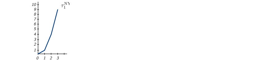
Figure 4: Cost tables, extending Figure 3, computed by the mechanism.

Given a node $a^{r}$, the first step of the algorithm is to select, for each node $c\in\textsl{ch}(r)$, the value $v_{c}^{0}$ with minimum cost, i.e., $v^{0}_{c}=\operatornamewithlimits{argmin}_{v}\bm{\tau}^{c}(v)$. As a result, the value $V^{0}=\sum_{c}v^{0}_{c}$ has minimal cost $\bm{\phi}^{r}(V^{0})=\sum_{c}\bm{\tau}^{c}(v^{0}_{c})$. Having constructed the minimum value in cost table $\bm{\phi}^{r}$, it remains to compute the costs of all values $V^{0}+k$ for all integer $k\in[1,\max D^{r}-V^{0}]$ and all values $V^{0}-k$ for all integer $k\in[1,V^{0}-\min D^{r}]$. The presentation focuses on the values $V^{0}+k$ since the two cases are similar. Let ${\bf{v}}^{0}=\{v^{0}_{c}\}_{c\in\textsl{ch}(r)}$. The algorithm builds a sequence of vectors ${\bf{v}}^{1},{\bf{v}}^{2},\ldots,{\bf{v}}^{k},\ldots$ that provides the optimal combinations of values for $\bm{\phi}^{r}(V^{0}+1),\bm{\phi}^{r}(V^{0}+2),\ldots,\bm{\phi}^{r}(V^{0}+k),\ldots$. Vector ${\bf{v}}^{k}$ is obtained from ${\bf{v}}^{k-1}$ by changing the value of a single child whose cost table has the smallest slope, i.e.,

$$v_{c}^{k}=\left\{\begin{array}[]{l l}v_{c}^{k-1}+1&\mbox{if }\;c=\operatornamewithlimits{argmin}_{c}\bm{\tau}^{c}(v_{c}^{k-1}+1)-\bm{\tau}^{c}(v_{c}^{k-1})\\ v_{c}^{k-1}&\mbox{otherwise.}\end{array}\right.$$ (7)

Once $\bm{\phi}^{r}$ has been computed, cost table $\bm{\tau}^{r}$ can be computed easily since both $(v-\tilde{n}^{r})^{2}$ and $\bm{\phi}^{r}$ are CPWL and the sum of two CPWL functions is CPWL. A full algorithm is described in the next section.

 Example​ 4

These concepts are illustrated in Figure 4, where the values of $\bm{\phi}^{r}$ are highlighted in blue, and in parenthesis, in the right table. The first step identifies that $v^{0}_{\textsl{NY}}=0$, $v^{0}_{\textsl{GA}}=3$, thus $V^{0}=3$ and $\bm{\phi}^{r}(3)=\bm{\tau}^{\textsl{NY}}(0)+\bm{\tau}^{\textsl{GA}}(3)=0+0=0$. In the example, ${\bf{v}}^{0}=(v^{0}_{\textsl{NY}},v^{0}_{\textsl{GA}})=(0,3)$ and ${\bf{v}}^{1}=(v^{1}_{\textsl{NY}},v^{1}_{\textsl{GA}})=(1,3)$, since $\textsl{NY}=\operatornamewithlimits{argmin}\{\bm{\tau}^{\textsl{NY}}(0+1)-\bm{\tau}^{\textsl{NY}}(0),\bm{\tau}^{\textsl{GA}}(3+1)-\bm{\tau}^{\textsl{GA}}(3)\}=\operatornamewithlimits{argmin}\{1-0,1-0\}$. Its associated cost, $\bm{\phi}^{\textsl{US}}({\bf{v}}^{1})=1+0=1$. ${\bf{v}}^{2}=(1,4)$ since $\textsl{GA}=\operatornamewithlimits{argmin}\{(\bm{\tau}^{\textsl{NY}}(1+1)-\bm{\tau}^{\textsl{NY}}(1)),(\bm{\tau}^{\textsl{GA}}(3+1)-\bm{\tau}^{\textsl{GA}}(3))\}=\operatornamewithlimits{argmin}\{(4-1),(1-0)\}$, and its associated cost $\bm{\phi}^{\textsl{US}}({\bf{v}}^{2})=1+1=2$.

 Theorem​ 3

The cost table $\bm{\tau}_{s}^{r}$ of each node $a_{s}^{r}$ of $\mathcal{T}^{\textsl{dp}}$ is CPWL.

7.1 Computing Cost Tables Efficiently

1

2

3${\bf{v}}^{+}\!\leftarrow\!\textsl{sort}^{2}(\langle c,\bm{\tau}^{c}(v)-\bm{\tau}^{c}(v-1)\rangle\>|\>c\!\in\!\textsl{ch}(r),v\!\in\!D^{c+})\!\!\!\!\!\!\!\!\!\!\!\!\!\!\!$

4 ${\bf{v}}^{-}\!\leftarrow\!\textsl{sort}^{2}(\langle c,\bm{\tau}^{c}(v)-\bm{\tau}^{c}(v-1)\rangle\>|\>c\!\in\!\textsl{ch}(r),v\!\in\!D^{c-})\!\!\!\!\!\!\!\!\!\!\!\!\!\!\!$

5 $\bm{\tau}^{r}\leftarrow\textnormal{{Merge}}(\textsl{extract}^{1}({\bf{v}}^{+}),+1,\bm{\tau}^{r})$

6 $\bm{\tau}^{r}\leftarrow\textnormal{{Merge}}(\textsl{extract}^{1}({\bf{v}}^{-}),-1,\bm{\tau}^{r})$

7Function Merge(${\bf{v}}$, $\kappa$, $\bm{\tau}^{r}$):

8       ${\bf{v}}[c]\leftarrow\operatornamewithlimits{argmin}\bm{\tau}^{c}\;\;\forall c\in\textsl{ch}(c)$

9       $v\leftarrow\sum_{c\in\textsl{ch}(r)}{\bf{v}}[c]$

10       if $\kappa>0\land v\in D^{r}$ then  $\bm{\tau}^{r}(v)\leftarrow\sum_{c\in\textsl{ch}(c)}\bm{\tau}^{c}({\bf{v}}[c])$

11       for $e\in{\bf{v}}$ do

12             ${\bf{v}}[e]\leftarrow{\bf{v}}[e]+\kappa$

13             $v\leftarrow\sum_{c\in\textsl{ch}(r)}{\bf{v}}[c]$

14             if $v\in D^{r}$ then  $\bm{\tau}^{r}(v)\leftarrow\sum_{c\in\textsl{ch}(r)}\bm{\tau}^{c}({\bf{v}}[c])$

15            

16       end for

17      return $\bm{\tau}^{r}$

18

Algorithm 1 TableMerge($a^{r}$)

The procedure to compute $\bm{\phi}_{s}^{r}$ is depicted in Algorithm 1: It is executed during the bottom-up phase of the dynamic program in lieu of Equations 4a, 4c, 4b and 4d. It takes as input the node $a^{r}$ and returns its associated cost function $\bm{\tau}^{r}$. Let $D^{c+}=\{v\>|\>v\in D^{c}\land v>\operatornamewithlimits{argmin}_{v^{\prime}}\bm{\tau}^{c}(v^{\prime})\}$ be the set of elements in the domain of $\bm{\tau}^{c}$ whose values are greater than the value corresponding to the table minimum cost. Similarly, let $D^{c-}=\{v\>|\>v\in D^{c}\land v<\operatornamewithlimits{argmin}_{v^{\prime}}\bm{\tau}^{c}(v^{\prime})\}$. Lines $1$ and $2$ construct the vectors ${\bf{v}}^{+}$ and ${\bf{v}}^{-}$ that list the pairs $(c,\bm{\tau}^{c}(v)-\bm{\tau}^{c}(v-1))$ of node identifier and slope associated with the cost function for every child node $a^{c}$ of $a^{r}$ and element $v\in D^{c+}$ (resp. $\in D^{c-}$), sorted using the second element of the pair. Lines $3$ and $4$ extract the identifiers for each element of the sorted lists ${\bf{v}}^{+}$ and ${\bf{v}}^{-}$ and call the function Merge to update the node cost function $\bm{\tau}^{r}$.

The heart of Algorithm 1 is the function Merge. For a node $\bm{\tau}^{r}$, it takes as input a sorted vector of the identifiers (containing as many elements as the sum of all children’s domain sizes), a value $\kappa\!\in\!\{+1,-1\}$, and the current node $\bm{\tau}^{r}$. Line $6$ constructs a map ${\bf{v}}$ that assigns to each children $a^{c}$ of $a^{r}$ the value associated with the minimum cost of its table $\bm{\tau}^{r}$. Line $7$ sums the values in the map ${\bf{v}}$ resulting in a value $v$ for which the function will compute the cost $\bm{\tau}^{r}$ of the parent node (line $8$). The conditional statement ensures that this operation is done only once–the Merge function is also called on vector ${\bf{v}}^{-}$. Next, for each element in the sorted vector ${\bf{v}}$, the function selects the next element $e$, it increases its current index ${\bf{v}}[e]$ by $\kappa$, and repeats the operations above, effectively computing the value $\bm{\tau}^{r}(v)$ for the cost table of node $a^{r}$. Line $12$ simply ensures that the computed value is in the domain of the node.

 Example​ 5

An example of the effect of Algorithm 1 executed on a few steps of the cost tables $\bm{\tau}_{1}^{\textsl{US}},\bm{\tau}_{1}^{\textsl{GA}},\bm{\tau}_{1}^{\textsl{NY}}$ is illustrated in Figure 4. Consider the computation of the cost function $\bm{\tau}_{1}^{\textsl{{US}}}$. We focus only on the first call of the Merge function. The algorithm first constructs the vector ${\bf{v}}^{+}=((\textsl{NY},1),(\textsl{GA},4),(\textsl{NY},2),(\textsl{GA},5),(\textsl{NY},3))$ (line 1), extracts its first component ${\bf{v}}^{+}=(\textsl{NY},\textsl{GA},\textsl{NY},\textsl{GA},\textsl{NY})$ (line 3), and hence calls the Merge function. The routine first initializes the vector ${\bf{v}}$ as ${\bf{v}}[\textsl{NY}]=\operatornamewithlimits{argmin}\bm{\tau}_{1}^{\textsl{NY}}=0,{\bf{v}}[\textsl{GA}]=\operatornamewithlimits{argmin}\bm{\tau}_{1}^{\textsl{GA}}=3$ (line 6), and $v={\bf{v}}[\textsl{NY}]+{\bf{v}}[\textsl{GA}]=0+3=3$ (line 7). It hence computes the value $\bm{\tau}_{1}^{\textsl{US}}(3)=1$ (line 8). Its associated cost is composed by the parent contribution (from Equation 4a) $|3-2|^{2}=1$ and the children contribution $\bm{\tau}_{1}^{\textsl{NY}}(0)=0$ and $\bm{\tau}_{1}^{\textsl{GA}}(3)=0$. Next, the algorithm increases $v$ by $1$ ($v=4$), in line 11, and selects the next element in ${\bf{v}}^{+}$ (i.e., "NY"), in line 9. It increments its value, ${\bf{v}}[\textsl{NY}]=1$ (line 10), and computes: $\bm{\tau}_{1}^{\textsl{US}}(4)=|4-2|^{2}+\bm{\tau}_{1}^{\textsl{NY}}({\bf{v}}[\textsl{NY}])+\bm{\tau}_{1}^{\textsl{GA}}({\bf{v}}[\textsl{GA}])=4+1+0=5$ (line 12). Finally, it increases $v$ by $1$ ($v=5$) and selects the next element in ${\bf{v}}^{+}$ (i.e., “GA"). It increments its value, ${\bf{v}}[\textsl{GA}]=1$ and computes: $\bm{\tau}_{1}^{\textsl{US}}(5)=|5-2|^{2}+\bm{\tau}_{1}^{\textsl{NY}}({\bf{v}}[\textsl{NY}])+\bm{\tau}_{1}^{\textsl{GA}}({\bf{v}}[\textsl{GA}])=9+1+1=11$.

 Theorem​ 4

The cost table $\bm{\tau}^{r}_{s}$ for each region $r$ and size $s$ can be computed in time $O\big{(}\bar{D}\log\bar{D}\big{)}$.

The result above can be derived observing that the runtime complexity of Algorithm 1 is dominated by the sorting operations in lines $1$ and $2$.

8 Cumulative Counts for Reduced Sensitivity

In the mechanisms presented so far, each query has sensitivity $\Delta_{\bm{n}}=2$. This section exploits the structure of the group query to reduce the query sensitivity and thus the noise introduced by the geometric mechanism. The idea relies on an operator $\oplus:\mathbb{Z}_{+}^{N}\to\mathbb{Z}_{+}^{N}$ that, given a vector $\bm{n}=(n_{1},\ldots,n_{N})$ of group sizes, returns its cumulative version $\bm{c}=(c_{1},\ldots,c_{N})$ where $c_{s}=\sum_{k=1}^{s}n_{k}$ is the cumulative sum of the first $s$ elements of $\bm{n}$.

 Lemma​ 6

The sensitivity $\Delta_{\bm{c}}$ of the cumulative group estimate query is 1.

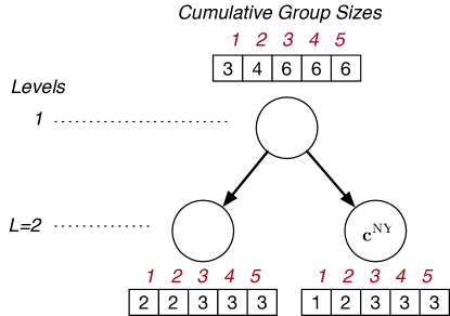
Figure 5: Cumulative group size hierarchy $\mathcal{T}_{2}^{c}$ associated with the dataset of Table 3.

The result follows from the fact that removing an element from a group $s$ in $\bm{c}$ only decreases group $s$ by one and increases the group $s-1$ preceding it by one. This idea is from [19], where cumulative sizes are referred to as unattributed histograms.

9 Cumulative PGSR Mechanisms

Operator $\oplus$ can be used to produce a hierarchy $\mathcal{T}^{c}=\{\bm{c}^{r}|r\in\mathcal{R}\}$ of cumulative group sizes. An example of such a hierarchy is provided in Figure 5. To generate a privacy-preserving version $\tilde{\mathcal{T}}^{c}$ of $\mathcal{T}^{c}$, it suffices to apply the geometrical mechanism with parameter $\lambda=(L/\epsilon)^{N}$ on the vectors $\bm{c}^{r}$ associated with every node $a_{s}^{r}$ for the groups of size $s$ in region $r$ of the region hierarchy. Once the noisy sizes are computed, the noisy group sizes can be easily retrieved via an inverse mapping $\ominus:\mathbb{Z}_{+}^{N}\to\mathbb{Z}_{+}^{N}$ from the cumulative sums.

Note, however, that the resulting private versions $\tilde{\bm{c}}^{r}$ of $\bm{c}^{r}$ may no longer be non-decreasing (or even non-negative) due to the added noise. Therefore, as in Section 5, a post-processing step is applied to restore consistency and to guarantee the PGSR conditions (2) to (4). The post-processing is illustrated in Model 2. It takes as input the noisy hierarchy of cumulative sizes $\tilde{\mathcal{T}}^{c}$ computed with the geometrical mechanism and optimizes over variables $\hat{\bm{c}}^{r}=(\hat{c}_{1}^{r},\ldots,\hat{c}_{N}^{r})$ for $r\in\mathcal{R}$, minimizing the L2-norm with respect to their noisy counterparts (Equation C1). Constraints (C2) guarantees that the sum of the sizes equals the public value $G$ (PGSR condition 4), where $\top$ denotes the root region of the region hierarchy. Constraints (C3) guarantee consistency of the cumulative counts. Finally, Constraints (C4) and (C5), respectively, guarantee the PGSR consistency (2) and validity (3) conditions.

Model 2 The $\mathcal{M}_{c}$ post-processing step.

$$\operatornamewithlimits{Minimize~{}}_{\left\{\hat{\bm{c}}^{r}\right\}_{r\in\mathcal{R}}}\;\; \sum_{r\in\mathcal{R}}\left\|\hat{\bm{c}}^{r}-\tilde{\bm{c}}^{r}\right\|_{2}^{2}$$ (C1)

$$\operatornamewithlimits{Subject~{}to:}\;\; \hat{c}^{\top}_{N}=G$$ (C2)

$$\hat{c}^{r}_{i}\leq\hat{c}^{r}_{i+1} \qquad\forall r\in\mathcal{R},i\in[N-1]$$ (C3)

$$\sum_{r^{\prime}\in\textsl{ch}(r)}\hat{c}^{r^{\prime}}_{i}=\hat{c}^{r}_{i} \qquad\forall r\in\mathcal{R},i\in[N]$$ (C4)

$$\hat{c}^{r}_{i}\in\{0,1,\ldots\} \qquad\forall r\in\mathcal{R},i\in[N]$$ (C5)

Once the post-processed hierarchy $\hat{\mathcal{T}}^{c}$ is obtained, the operator $\ominus$ is applied to obtain a post-processed version of the group size hierarchy $\hat{\mathcal{T}}$. The resulting mechanism, denoted by $\mathcal{M}_{c}$ is called the Cumulative PGSR Mechanism. $\mathcal{M}_{c}$ satisfies $\epsilon$-differential privacy, due to post-processing immunity, similarly to the argument presented in Theorem 1 (see Appendix). This mechanism is called the cumulative PGSR and denoted by $\mathcal{M}_{c}$.

1

input : $\tilde{\mathcal{T}}^{c}=\{\tilde{\bm{c}}^{r}\>|\>r\in\mathcal{R}\}$

2 foreach $r\in\mathcal{R}$ do

3       $\displaystyle\hat{\bm{c}}^{r}\leftarrow\hskip 16.0pt\operatornamewithlimits{argmin}_{\hat{\bm{c}}}\;\;\left\|\hat{\bm{c}}-\tilde{\bm{c}}^{r}\right\|^{2}$

       $\hskip 25.0pt\displaystyle\operatornamewithlimits{Subject~{}to:}\;\;\hat{c}_{i}\leq\hat{c}_{i+1}\qquad\;\;\;\forall i\in[N-1]$

       $\hskip 80.0pt0\leq\hat{c}_{i}\leq G\qquad\forall i\in[N]$

4       $\bar{\bm{n}}\leftarrow\ominus(\textsl{round}(\hat{\bm{c}}^{r}))$

5       $\hat{\mathcal{T}}\leftarrow\bar{\mathcal{T}}\cup\{\bar{\bm{n}}\}$

6 end foreach

$\hat{\mathcal{T}}\leftarrow\mathcal{M}_{\textsl{dp}}.{\textsl{post-process}}(\hat{\mathcal{T}})$

Algorithm 2 $\mathcal{M}_{c}^{\textsl{dp}}$.post-process

9.1 An Approximate Dynamic Programing Cumulative PGSR Mechanisms

Unlike for $\mathcal{M}_{H}$, the structure of the PGSR problem cannot be exploited directly to create a dynamic-programming mechanism. The constraints imposed by the optimization in Model 2 do not allow for a hierarchical decomposition with recurrent substructure as the inequalities (C3) relate sibling nodes in the hierarchy. Therefore, a dynamic program that exploits the dependencies induced by the region hierarchy $\mathcal{T}$, would need to associate each node $a^{r}$ in $\mathcal{T}$ with a cost table $\bm{\tau}^{r}$ which may take as input vectors of size up to $N$. It follows that each cost table $\bm{\tau}^{r}$ size is in $O(\binom{G+N-1}{N-1})$, which makes this dynamic-programming approach computationally intractable, especially for real-world applications.

To address this issue, a previous version of this work [15], proposed an approximated dynamic program version of the cumulative mechanism, called $\mathcal{M}_{c}^{\textsl{dp}}$ that operates in three steps:

1. It creates a noisy hierarchy $\tilde{\mathcal{T}}^{c}$.

2. Next, it executes the post-processing step described in Algorithm 2.

3. Finally, it runs the post-processing step of the polynomial-time PGSR mechanism (see Section 7).

The important addition is in step 2 which takes $\tilde{\mathcal{T}}^{c}$ as input and, for each node $\tilde{\bm{c}}^{r}$, solves the convex program described in line 2 of Algorithm 2 to create a new noisy hierarchy $\hat{\bm{c}}^{r}$ that is non-decreasing and non-negative. The resulting cumulative vector $\hat{\bm{c}}^{r}$ is then rounded and transformed to its corresponding group size vector through operator $\ominus(\cdot)$ (line 3). The resulting vector $\bar{\bm{n}}^{r}$ is added to the region hierarchy $\hat{\mathcal{T}}$ (line 4). Observe that this post-processing step pays a polynomial-time penalty with respect to the runtime of the $\mathcal{M}_{H}^{\textsl{dp}}$ post-processing. The convex program of line (2) is executed in $O(\text{poly}(N))$ and the resulting post-processing step runtime is in $O\big{(}|\mathcal{R}|\text{poly}(N)+|\mathcal{R}|N\bar{D}\log\bar{D}\big{)}$.

While, the experimental results (see Section 11) show that $\mathcal{M}_{c}^{\textsl{dp}}$ consistently reduces the final error, when compared to $\mathcal{M}_{H}^{\textsl{dp}}$, it is important to note that $\mathcal{M}_{c}^{\textsl{dp}}$ does not solve the same post-processing program as the cumulative PGSR mechanism specified by Equations C1, C5, C3, C4 and C2, since it restores consistency of the cumulative counts locally. To address this issue, this work introduces next an exact DP cumulative PGSR mechanism.

9.2 An Exact Dynamic Programming Cumulative PGSR Mechanisms

This section develops an exact and efficient dynamic programming algorithm for solving the cumulative PGSR problem optimally. It relies on the observation that, when the cumulative operator $\oplus$ is applied to the hierarchy $\mathcal{T}^{\textsl{dp}}$ instead than to the original hierarchy $\mathcal{T}$, the post-processing step of Model 2 only imposes inequalities among sibling nodes within each subtree, allowing the construction of overlapping sub-problems.

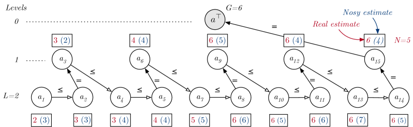
Figure 6: The $\mathcal{T}^{\textsl{ch}}$ node ordering associated with the dataset of Table 3.

More precisely, the key insight is to build a chain of nodes by visiting the tree hierarchy $\mathcal{T}^{\textsl{dp}}$ (see Figure 3) using a post-order traversal. The resulting chain structure $\mathcal{T}^{\textsl{ch}}$ is composed of $|\mathcal{R}|\,N$ nodes, where $a_{i}$ refers to the $i$-th node in the post-order traversal of $\mathcal{T}^{\textsl{dp}}$. This chain structure enables the use of an efficient dynamic-programming algorithm to solve the post-processing step over cumulative counts. The resulting mechanism is referred to as the Chain-based Cumulative Dynamic Programming PGSR mechanism and denoted by $\mathcal{M}_{c}^{\textsl{ch}}$. It operates in three phases described as follows.

9.2.1 Cumulative Hierarchy Pre-processing Phase

Given a DP hierarchy $\mathcal{T}^{\textsl{dp}}$, the algorithm constructs a chain $\mathcal{T}^{\textsl{ch}}=\{c_{i}\mid i\in[|\mathcal{R}|N]\}$ by traversing the nodes of $\mathcal{T}^{\textsl{dp}}$ using a post-ordering scheme. Denote with $a_{i}$ and $n_{i}$ the $i$-th node and group size value, respectively, in the post-order traversal of $\mathcal{T}^{\textsl{dp}}$. The cumulative count $c_{i}$ associated with node $a_{i}$ is the sum of $n_{i}$ and all values $n_{j}$ associated with nodes $a_{j}$ that precedes $a_{i}$ and lie in the same level as $a_{i}$ in $\mathcal{T}^{\textsl{dp}}$. More formally,

$$c_{i}=\sum_{j\in S_{i}}n_{j}\,,\qquad S_{i}=\left\{j\mid j\leq i,~{}\text{lev}(a_{j})=\text{lev}(a_{i})\right\}\,,$$

where $\text{lev}(a)$ describes the level of node $a$ in $\mathcal{T}^{\textsl{dp}}$. An illustration of the chain structure $\mathcal{T}^{ch}$ associated with the running example is shown in Figure 6.

9.2.2 Privacy Phase

Next, the algorithm constructs a noisy version of the $\mathcal{T}^{\textsl{ch}}$ hierarchy, denoted $\tilde{\mathcal{T}}^{\textsl{ch}}$ that is constructed by applying the geometrical mechanism with parameter $\lambda(L/\epsilon)^{|\mathcal{R}_{\ell}|\,N}$ to the cumulative count vector $\bm{c}^{\ell}$ associated with the nodes at level $\ell$ for all $\ell\in[L]$. Figure 6 illustrates the resulting cumulative group values after the privacy-preserving phase in blue.

9.2.3 The Post-processing Phase

Given a noisy version $\tilde{\bm{c}}^{\ell}$ of the cumulative group sizes, an application of the inverse mapping $\ominus$ on $\tilde{\bm{c}}^{\ell}$ for each level $\ell\in[L]$ is sufficient to retrieve the desired noisy group sizes. However, the resulting group sizes may not satisfy the PGSR validity and consistency conditions. The third phase of $\mathcal{M}_{c}$ is a post-processing step to restore the PGSR conditions 2 to 4.

Model 3 The modified post-processing step.

Let $\dot{N}=|\mathcal{R}|\,N$

$$\operatornamewithlimits{Minimize~{}}_{\{\hat{c}_{i}\}_{i\in[\dot{N}]}}\;\; \sum_{i=1}^{\dot{N}}\|\hat{c}_{i}-\tilde{c}_{i}\|_{2}^{2}$$ (C6)

$$\operatornamewithlimits{Subject~{}to:}\;\; \hat{c}_{\dot{N}}=G$$ (C7)

$$\hat{c}_{i}\leq\hat{c}_{i+1} \qquad\forall i\in\left\{i\in[\dot{N}-1]\mid\text{lev}(a_{i})=\text{lev}(a_{i+1})\right\}$$ (C8)

$$\hat{c}_{i}=\hat{c}_{i+1} \qquad\forall i\in\left\{i\in[\dot{N}-1]\mid\text{lev}(a_{i})>\text{lev}(a_{i+1})\right\}$$ (C9)

$$\hat{c}_{i}\in\{0,1,\ldots\} \qquad\forall i\in[\dot{N}]$$ (C10)

This step is illustrated in Model 3. It aims at generating a new chain $\hat{\mathcal{T}}^{\textsl{ch}}$ whose counts are close to their noisy counterparts (C6) and satisfy the faithfulness (C7), consistency (C8) and (C9), and validity conditions (C10). Once the post-processed chain $\hat{\mathcal{T}}^{\textsl{ch}}$ is obtained, the operator $\ominus$ is applied to obtain the corresponding version of the group size hierarchy $\hat{\mathcal{T}}$.

The advantage of this formulation is its ability to exploit the chain structure $\mathcal{T}^{\textsl{ch}}$ associated with the region hierarchy $\mathcal{T}^{\textsl{dp}}_{c}$, via an efficient dynamic programming algorithm to solve the post-processing step. Similarly to $\mathcal{M}_{H}^{\textsl{dp}}$, this dynamic program consists of two phases, a bottom-up and a top-down phase, corresponding to the direction in which the chain is traversed.

In the bottom-up phase, each node $a_{i}$ of $\mathcal{T}^{\textsl{ch}}$ constructs a cost table $\bm{\tau}_{i}:D_{i}\to\mathbb{R}_{+}$, where $D_{i}\subseteq\mathbb{N}$ is the domain associated with node $a_{i}$, mapping values to costs. Intuitively, the cost table $\bm{\tau}_{i}(v)$ represents the optimal cost for the first $i$ nodes when the post-processed cumulative group size of the node $a_{i}$ is equal to $v$. The cost tables for all nodes are updated starting from the head of the chain to its tail, according to the following recurrence relationship:

$$\bm{\tau}_{i+1}(v)= \left(v-\tilde{c}_{i+1}\right)^{2} +$$ (8a)

$$\hskip 20.0pt\bm{\phi}_{i+1}(v) =\begin{cases}\bm{\tau}_{i}(v)&\text{if }\mathrm{lev}(a_{i})>\text{lev}(a_{i+1}),\\ \underset{\begin{subarray}{c}x_{i}\in D_{i}\\ x_{i}\leq v\end{subarray}}{\operatornamewithlimits{Minimize~{}}}\bm{\tau}_{i}(x_{i})&\mathrm{otherwise.}\end{cases}$$ (8b)

The formulation for the cost $\bm{\tau}_{i+1}(v)$ has two components. The first component captures the deviation of the post-processed value $v$ from the noisy cumulative group size $\tilde{c}_{i+1}$ (Equation 8a). The second component captures the optimal post-processing cost associated with the first $i$ nodes of the chain, provided that the succeeding node $a_{i+1}$ takes on value of $v$ (Equation 8b).

In the top-down phase, the algorithm traverses each node from the tail of the chain to its head. The node $\hat{c}_{|\mathcal{R}|N}$ is set to value $G$ (to satisfy Constraint (C7)). Each visited node $a_{i+1}$, for any $i\in[|\mathcal{R}|N-1]$, receives the post-processed cumulative group size $\hat{c}_{i+1}$ and determines the optimal post-processed solution for its predecessor $a_{i}$ by solving $\bm{\phi}_{i+1}(\hat{c}_{i+1})$ given in (8b).

 Example​ 6

An example of the mechanism $\mathcal{M}_{c}^{\textsl{ch}}$ executed on a few steps of the cost tables $\bm{\tau}_{1}^{\textsl{GA}},\bm{\tau}_{1}^{\textsl{NY}},\bm{\tau}_{1}^{\textsl{US}}$ is shown in Table 6. Consider the computation of the

$\bm{v}$ $\tau_{1}^{\textsl{GA}}$ $\tau_{1}^{\textsl{NY}}$ $\bm{0}$ 9 $9\!+\!9$ $=\!\min(9)$ $\bm{1}$ 4 $4\!+\!4$ $=\!\min(9,4)$ $\bm{2}$ 1 $1\!+\!1$ $=\!\min(0,4,1)$ $\bm{3}$ ${}^{*}0$ ${}^{*}0\!+\!0$ $=\!\min(9,4,1,0)$ $\bm{4}$ 1 $1\!+\!0$ $=\!\min(9,4,1,0,1)$ $\bm{v}$ $\tau_{1}^{\textsl{NY}}$ $\tau_{1}^{\textsl{US}}$ $\bm{0}$ 18 $4\!+\!18$ $\bm{1}$ 8 $1\!+\!8$ $\bm{2}$ 2 $0\!+\!2$ $\bm{3}$ ^∗0 ${}^{*}1\!+\!0$ $\bm{4}$ 1 $4\!+\!1$

Table 6: Example of cost table computation for subtree associated to the group 1 estimates.

cost function $\bm{\tau}_{1}^{\textsl{US}}$ in the bottom-up phase. To start with, the algorithm initializes the cost table $\bm{\tau}_{1}^{\textsl{GA}}$ as $\bm{\tau}_{1}^{\textsl{GA}}(v)=\left|v-3\right|^{2}$, where the noisy cumulative group size associated with the node $a_{1}^{\textsl{GA}}$ is $3$. Notice that the post-processed cumulative group size of this node $a_{1}^{\textsl{GA}}$ is not supposed to exceed that of its succeeding node $a_{1}^{\textsl{NY}}$. Thus, the algorithm updates the cost table $\bm{\tau}_{1}^{\textsl{NY}}$ by aggregating the following two parts: The one including the cost associated with the current node $\left|v-3\right|^{2}$ and the that including the optimal cost for its preceding node(s) $\min_{0\leq x\leq v}\bm{\tau}_{1}^{\textsl{GA}}(x)$. It follows that $\bm{\tau}_{1}^{\textsl{NY}}(3)=\left|3-3\right|^{2}+\min_{0\leq x\leq 3}\bm{\tau}_{1}^{\textsl{GA}}(x)=0+\bm{\tau}_{1}^{\textsl{GA}}(3)=0+0=0$. Then, for the node $a_{1}^{\textsl{US}}$, its post-processed cumulative group size equals that of its preceding node $a_{1}^{\textsl{NY}}$. As a result, its associated cost, say $\bm{\tau}_{1}^{\textsl{US}}(3)$, is composed by $\left|3-2\right|^{2}=1$ and $\bm{\tau}_{1}^{\textsl{NY}}(3)=0$. The table marks the value selected during the top-down phase with a ^∗ symbol.

The next results discuss the piecewise linear convexity of the cost function $\bm{\phi}$ and the computational complexity of the algorithm.

 Lemma​ 7

The cost table $\bm{\tau}_{i}$ of each node $a_{i}$ of $\mathcal{T}^{\textsl{ch}}$ is CPWL.

 Theorem​ 5

The cost table $\bm{\tau}_{i}$ for each $i\in[|\mathcal{R}|N]$ can be computed in time $O\big{(}\bar{D}\big{)}$, where $\bar{D}=\max_{i}|D_{i}|$ for $i\in[|\mathcal{R}|N]$.

10 Related Work

The release of privacy-preserving datasets using differential privacy has been subject of extensive research [20, 25, 23]. These methods focus on creating unattributed histograms that count the number of individuals associated with each possible property in the dataset universe. During the years, more sophisticated algorithms have been proposed, including those exploiting the problem structure using optimization to improve accuracy [7, 23, 27, 24].

Additional extensions to consider hierarchical problems were also explored. Hay et al. [19] and Qardaji et al. [27] study methods to answer count queries over ranges using a hierarchical structure to impose consistency of counts. While hierarchies contribute an additional level of fidelity for realizing a realistic data release it further challenge the privacy/accuracy tradeoff. Other methods have also incorporated partitioning scheme to the data-release problem to further increase the accuracy of the privacy-preserving data by cleverly splitting the privacy budget in different hierarchical levels [32, 8, 33].

These methods differ in two ways from the mechanisms proposed here: (1) They focus on histograms queries, rather than group queries; the latter generally have higher $L_{1}$-sensitivity and thus require more noise and (2) they ensure neither the consistency for integral counts nor the non-negativity of the release counts. They thus violate the requirements of group sizes (see Section 4).

Fioretto and Van Hentenryck recently proposed a hierarchical-based solution based on minimizing the L2-distance between the noisy counts and their private counterparts [13]. While this solution guarantees non-negativity of the counts, their mechanism, if formulated as a MIP/QIP, cannot cope with the scale of the census problems discussed here which compute privacy-preserving country-wise group sizes. If their solution is used as is, in its relaxed form, then it cannot guarantee the integrality of the counts. These mechanisms reduce to $\mathcal{M}_{H}^{r}$, which, has is shown to be strongly dominated by the DP-based mechanisms (see Section 11).

A line of work that is closely related to the problem analyzed in this paper is that initiated by Blocki et al. [6] and Hay et al. [19] that study unattributed histogram which are often used to study node degrees in a path in graphs. Unattributed histograms are used to answer queries of the type: “How many people belong to the $k$-th largest group?”. They can be far more accurate than naively adding noise to each group and then selecting the $k$-th largest noisy group [19]. They are however different from the queries used in this work as they count people rather then groups and are not necessarily hierarchical. A substantial contribution is represented by the work of Kui et al. [21], that study the problem of releasing hierarchical group queries that satisfies the non-negativity, integrality, and consistency of the counts. They propose a solution that, similarly to [13], can be mapped to $\mathcal{M}_{H}^{r}$ and apply rounding to ensure integrality, as well as studying the context of cumulative group queries.

Finally, an important deployment is represented by the TopDown algorithm [5], used by the US Census to for the 2018 end-to-end test, in preparation for the 2020 release. The algorithm is a weaker form of $\mathcal{M}_{H}^{r}$ that first obtains inexact noisy counts to satisfy the desired privacy level and then alternates the following two steps for multiple levels of a geographic hierarchy, from top to bottom, as the name suggests. The first step is a program analogous to $\mathcal{M}_{H}^{r}$, but it operates on two consecutive levels only. The second step is an ad-hoc rounding strategy to guarantee the integrality of the counts while satisfying the hierarchical invariants. These two steps are repeated processing two contiguous levels of the hierarchy until the leaves are reached.

11 Experimental Evaluation

This section evaluates the proposed privacy-preserving mechanisms for the PGSR problem. The evaluation focuses on comparing runtime and accuracy of the mechanisms described in the paper. Consistent with the privacy literature, accuracy is measured in term of the $L_{1}$ difference between the privacy-preserving group sizes and the original ones, i.e., given the original group sizes $\mathcal{T}=\{\bm{n}^{r}\>|\>r\in\mathcal{R}\}$, and their private counterparts $\hat{\mathcal{T}}$, the $L_{1}$-error is defined as $\sum_{r}\|\bm{n}^{r}-\hat{\bm{n}}^{r}\|_{1}$. Since the mechanisms are non-deterministic due to the noise added by the geometric mechanism, $30$ instances are generated for each benchmark and the results report average values and standard deviations. Each mechanism is run on a single-core $2.1$ GHz terminal with $24$GB of RAM and is implemented in Python $3$ with Gurobi $8.1$ for solving the convex quadratic optimization problems.

Mechanisms

The evaluation compares the PGSR mechanisms $\mathcal{M}_{H}$, its cumulative version $\mathcal{M}_{c}$, and their polynomial-time dynamic-programming (DP) counterparts $\mathcal{M}_{H}^{\textsl{dp}}$, $\mathcal{M}_{c}^{\textsl{dp}}$, and $\mathcal{M}_{c}^{\textsl{ch}}$. The former are referred to as OP-based methods and the latter as DP-based methods. In addition to $\mathcal{M}_{H}$ and $\mathcal{M}_{c}$, that solve the associated post-processing QIPs, the experiments evaluate the associated relaxations, $\mathcal{M}_{H}^{r}$ and $\mathcal{M}_{c}^{r}$, respectively, that relax the integrality constraints (H4) and (C5) and rounds the solutions. still guaranteeing non-negativity and the final solutions are rounded. For completeness, the experiments also evaluate the performance of the TopDown algorithm [5] and the optimization-based mechanism $\mathcal{M}_{\textsl{dp}}^{\text{OP}}$ that does not exploit the structure of the cost function to compute the cost tables.

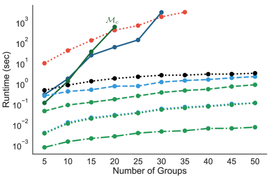
Figure 7: Runtime (in seconds) at varying of the number of group size $N$.

Datasets

The mechanisms are evaluated on three datasets.

• Census Dataset: The first dataset has 117,630,445 groups, 7,592 leaves, 305,276,358 individuals, 3 levels, and $N$=1,000. Individuals live in facilities, i.e., households or dormitories, assisted living facilities, and correctional institutions. Due to privacy concerns and lack of available methods to protect group sizes during the 2010 Decennial Census release, group sizes were aggregated for any facility of size 8 or more (see Summary File 1 [30]). Therefore, following [22] and starting from the truncated group sizes Census dataset, the experiments augment the dataset with group sizes up to $N$=1,000 that mimic the published statistics, but add a heavy tail to model group quarters (dormitories, correctional facilities, etc.). This was obtained by computing the ratio $r=n_{7}/n_{6}$ of household groups of sizes 7 and 6, subtracting from the aggregated groups $n_{8+}$ $M$ people according to the ratio $r$, and redistributed these $M$ people in groups $k>8$ so that the ratio between any two consecutive groups holds (in expectation). Finally, $50$ outliers were added, chosen uniformly in the interval between $10$ and $1,000$. The region hierarchy is composed by the National level, the State levels (50 states + Puerto Rico and District of Columbia), and the Counties levels (3144 in total).

• NY Taxi Dataset: The second dataset has 13,282 groups, 3,973 leaves, 24,489,743 individuals, 3 levels, and $N$=13,282. The 2014 NY city Taxi dataset [3] describes trips (pickups and dropoffs) from geographical locations in NY city. The dataset views each taxi as a group and the size of the group is the number of pickups of the taxi. The region hierarchy has 3 levels: the entire NY city at level 1, the boroughs: Bronx, Brooklyn, EWR, Manhattan, Queens, and Staten Island at level 2, and a total of 263 zones at level 3.

• Synthetic Dataset: Finally, to test the runtime scalability, the experiments considered synthetic data from the NY Taxi dataset by limiting the number of group sizes $N$ arbitrarily, i.e., removing group sizes greater than a certain threshold.

11.1 Scalability

The first results concern the scalability of the mechanisms, which are evaluated on the synthetic datasets for various numbers of group sizes. Figure 7 illustrates the runtimes of the algorithms at varying of the number of group sizes $N$ from $5$ to $50$ for the synthetic dataset. The experiments have a timeout of $30$ minutes and the runtime is reported in log-$10$ scale. The figure shows that the exact OP-based approaches and $\mathcal{M}_{\textsl{dp}}^{\text{OP}}$ are not competitive, even for small groups sizes. Therefore, these results rule out the following mechanisms: $\mathcal{M}_{\textsl{dp}}^{\text{OP}}$, $\mathcal{M}_{H}$, and $\mathcal{M}_{c}$ and the remaining results focus on comparing the relaxed versions of the OP-based mechanisms versus their proposed DP-counterparts.

11.2 Runtimes

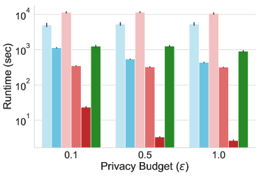
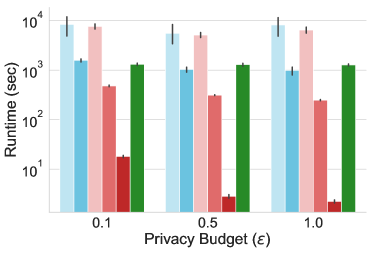
Figure 8: The Runtime for the mechanisms: Census data (left) and Taxi data (right).

Figure 8 reports the runtime, in seconds, for the hierarchical mechanism $\mathcal{M}_{H}^{r}$ and its DP-counterpart $\mathcal{M}_{H}^{\textsl{dp}}$, and the hierarchical cumulative mechanism $\mathcal{M}_{c}^{r}$ and its DP-counterpart $\mathcal{M}_{c}^{\textsl{dp}}$, together with $\mathcal{M}_{c}^{\textsl{ch}}$ and TopDown. The left figure illustrates the results for the Census data and the right one for the NY Taxi data. The main observations can be summarized as follows:

1. Although the OP-based algorithms consider only a relaxation of the problem, the exact DP-versions are consistently faster. In particular, $\mathcal{M}_{H}^{\textsl{dp}}$ is up to one order of magnitude faster than its counterpart $\mathcal{M}^{r}$, and $\mathcal{M}_{c}^{\textsl{dp}}$ is up to two orders of magnitude faster than its counterpart $\mathcal{M}_{c}^{r}$.

2. The proposed DP-based mechanisms are always faster than the TopDown algorithm and the newly proposed proposed $\mathcal{M}_{c}^{r}$ mechanism is up to two order of magnitude faster than TopDown.

3. $\mathcal{M}_{c}^{r}$ is consistently slower then $\mathcal{M}_{H}^{r}$. This is because, despite the fact that the two post-processing steps have the same number of variables, the $\mathcal{M}_{c}$ post-processing step has many additional constraints of type (C3).

4. The runtime of the DP-based mechanisms decreases as the privacy budget increases, due to the sizes of the cost tables that depend on the noise variance.

5. The cumulative version $\mathcal{M}_{c}^{\textsl{dp}}$ outperforms its $\mathcal{M}_{H}^{\textsl{dp}}$ counterpart. Once again, the reason is due to the domain sizes. In fact, due to reduced sensitivity, $\mathcal{M}_{c}^{\textsl{dp}}$ applies a smaller amount of noise than that required by $\mathcal{M}_{H}^{\textsl{dp}}$ to guarantee the same level of privacy and resulting in smaller domain sizes.

6. $\mathcal{M}_{c}^{\textsl{ch}}$ is consistently faster than $\mathcal{M}_{c}^{\textsl{dp}}$, which results from that computing the cost tables of the former is achieved with fewer operations than for the latter, as analyzed in Theorem 4 and Theorem 5.

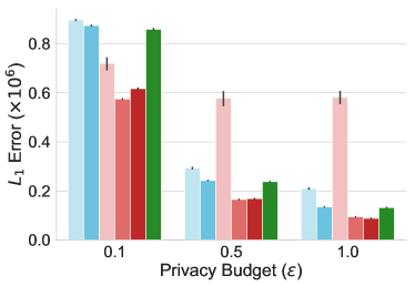
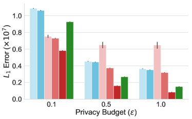
Figure 9: The $L_{1}$ errors for the algorithms: Census data (left) and Taxi data (right).

11.3 Accuracy

Figure 9 reports the error induced by the mechanisms, i.e., the $L_{1}$-distance between the privacy-preserving and original datasets. The main observations can be summarized as follows:

1. The DP-based mechanisms produce more accurate results than their counterparts and $\mathcal{M}^{\textsl{ch}}_{c}$ dominates all other mechanisms, including TopDown.

2. As expected, the error of all mechanisms decreases as the privacy budget increases, since the noise decreases as privacy budget increases. The errors are larger in the NY Taxi dataset, which has a larger number of group sizes than the Census dataset.

3. Finally, the results show that the cumulative mechanisms tend to concentrate the errors on small group sizes. Unfortunately, these are also the most populated groups, and this is true for each subregion of the hierarchy. On the other hand, the DP-based version, that retains the integrality constraints, better redistributes the noise introduced by the geometrical mechanism and produce substantially more accurate results.

To shed further light on accuracy, Table 7 reports a breakdown of the average errors of each mechanism at each level of the hierarchies. Mechanism $\mathcal{M}^{\textsl{ch}}_{c}$ is clearly the most accurate. Note that the table reports the average number of constraint violations in the output datasets. A constraint violation is counted whenever a subtree of the hierarchy violates the PGSR consistency condition (2). Being exact, the DP-based methods report no violations. In contrast, both $\mathcal{M}_{H}^{r}$ and $\mathcal{M}_{c}^{r}$ report a substantial amount of constraint violations.

	Taxi Data					Census Data
		$L_{1}$ Errors $(\times 10^{4})$			#CV	$L_{1}$ Errors $(\times 10^{3})$			#CV
$\epsilon$	Alg	Lev 1	Lev 2	Lev 3		Lev 1	Lev 2	Lev 3
0.1	$\mathcal{M}_{H}^{r}$	25.4	158.7	904.4	18206	40.3	54.3	802.1	1966
	$\mathcal{M}_{H}^{\textsl{dp}}$	26.6	121.9	915.7	0	10.3	38.4	825.4	0
	$\mathcal{M}_{c}^{r}$	47.9	153.2	551.6	19460	23.1	64.5	632.2	1715
	$\mathcal{M}_{c}^{\textsl{dp}}$	19.9	65.6	644.3	0	0.9	23.2	550.6	0
	$\mathcal{M}_{c}^{\textsl{ch}}$	5.5	39.3	537.8	0	0.2	13.9	603.0	0
	TopDown	26.6	93.0	809.1	0	3.7	35.0	820.5	0
0.5	$\mathcal{M}_{H}^{r}$	8.6	81.2	364.2	18591	39.4	37.9	216.3	1990
	$\mathcal{M}_{H}^{\textsl{dp}}$	5.5	31.0	408.9	0	2.4	9.4	230.8	0
	$\mathcal{M}_{c}^{r}$	46.7	153.5	450.7	19531	23.1	61.0	494.2	1718
	$\mathcal{M}_{c}^{\textsl{dp}}$	4.0	16.4	352.9	0	0.2	5.8	159.1	0
	$\mathcal{M}_{c}^{\textsl{ch}}$	1.2	9.5	150.6	0	0.0	3.4	165.3	0
	TopDown	5.3	20.3	242.1	0	0.9	8.6	228.4	0
1.0	$\mathcal{M}_{H}^{r}$	7.7	77.2	279.0	18085	40.7	39.2	130.0	1989
	$\mathcal{M}_{H}^{\textsl{dp}}$	3.1	19.8	328.5	0	1.2	5.1	128.8	0
	$\mathcal{M}_{c}^{r}$	47.1	154.2	447.1	19706	24.1	63.0	494.5	1728
	$\mathcal{M}_{c}^{\textsl{dp}}$	2.0	8.7	307.8	0	0.1	3.2	91.0	0
	$\mathcal{M}_{c}^{\textsl{ch}}$	0.5	4.5	78.6	0	0.0	1.7	86.9	0
	TopDown	2.6	10.3	138.4	0	0.5	4.6	127.2	0

Table 7: $L_{1}$-errors and constraint violations (CV) for each level of the hierarchies.

12 Conclusions

The release of datasets containing sensitive information concerning a large number of individuals is central to a number of statistical analysis and machine learning tasks. Of particular interest are hierarchical datasets, in which counts of individuals satisfying a given property need to be released at different granularities (e.g., the location of a household at a national, state, and county levels). The paper discussed the Privacy-preserving Group Release (PGRP) problem and proposed an exact and efficient constrained-based approach to privately generate consistent counts across all levels of the hierarchy. This novel approach was evaluated on large, real datasets and results in speedups of up to two orders of magnitude, as well as significant improvements in terms of accuracy with respect to state-of-the-art techniques. Interesting avenues of future directions include exploiting different forms of parallelism to speed up the computations of the dynamic programming-based mechanisms even further, using, for instance, Graphical Processing Units as proposed in [14].

Appendix A Missing Proofs

 Lemma​ 4

The sensitivity $\Delta_{\bm{n}}$ of the group estimate query is 2.

Proof. Consider a group size $\bm{n}$ (stripped of the superscript $r$ for notation convenience) derived by a dataset $D$ and let $\bm{n}^{\prime}$ be the group size generated by a neighboring dataset $D^{\prime}$ of $D$. Let $D^{\prime}=D\cup\{(p,u,r,1)\}$ be the dataset that adds an individual to some group $G_{u}$, for some $u\in\mathcal{U}$, associated with a group size $n_{i}$. This action decreases the group size $n_{i}$ value by one and increases the group size $n_{i+1}$ value by one, i.e., $n_{i}^{\prime}=n_{i}+1$ and $n_{i+1}^{\prime}=n_{i+1}-1$. Therefore $\|\bm{n}^{\prime}-\bm{n}\|_{1}=2$. A similar argument applies to a neighboring dataset that removes an individual from $D$. $\Box$

 Theorem​ 1

$\mathcal{M}_{H}$ satisfies $\epsilon$-differential privacy.

Proof. First note that each level of the hierarchy forms a partition over the regions in $\mathcal{R}$ (by definition of hierarchy). By parallel composition (Lemma 2), for each level $\ell\in[L]$, the noisy values $\tilde{\bm{n}}^{r}$ for all $r\in\mathcal{R}_{\ell}$ satisfy $\frac{\epsilon}{L}$-differential privacy. There are exactly $L$ levels in the hierarchy: Therefore, by sequential composition (Lemma 1), the mechanism satisfies $\epsilon$-differential privacy. $\Box$

 Theorem​ 2

Constructing $\hat{\mathcal{T}}^{\textsl{dp}}$ requires solving $O(|\mathcal{R}|\,N\,\bar{D}$) optimization problems given in Equation 4, where $\bar{D}=\max_{s,r}|D_{s}^{r}|$ for $r\in\mathcal{R},s\in[N]$.

Proof. There are exactly $|\mathcal{R}|N$ nodes, and each node runs the program in Equation 4 for each element of its domain $D_{s}^{r}$. $\Box$

The next lemma is the key technical result of the paper and it requires some additional notation. Let $(v_{0},\ldots,v_{n})$ be the ordered sequence of values in $D^{r}$, i.e., $v_{i+1}=v_{i}+1$ for all $i=0\ldots n-1$. Given a cost table $\bm{\tau}^{r}$, its associated cost function $\mathring{\bm{\tau}}^{r}$ is a PWL function defined for all $x\in[v_{0},v_{n}]$ as:

$$\mathring{\bm{\tau}}^{r}(x)=\left\{\begin{array}[]{l l}(x-v_{0})(\bm{\tau}^{r}(v_{1})-\bm{\tau}^{r}(v_{0}))+\bm{\tau}^{r}(v_{0})&\text{if }v_{0}\leq x<v_{1}\\ (x-v_{1})(\bm{\tau}^{r}(v_{2})-\bm{\tau}^{r}(v_{1}))+\bm{\tau}^{r}(v_{1})&\text{if }v_{1}\leq x<v_{2}\\ \ldots&\\ (x-v_{n-1})(\bm{\tau}^{r}(v_{n})-\bm{\tau}^{r}(v_{n-1}))+\bm{\tau}^{r}(v_{n-1})&\text{if }v_{n-1}\leq x\leq v_{n}.\end{array}\right.$$ (9)

Similarly, $\mathring{\bm{\phi}}^{r}$ is the PWL function defined from $\bm{\phi}^{r}$ by the same process.

 Lemma​ 5

Consider a given region $r$ and group size $s$. If $\mathring{\bm{\tau}}_{s}^{c}$ is CPWL for all $c\in ch(r)$, then $\mathring{\bm{\phi}}^{r}_{s}$ is CPWL.

Proof. For simplicity, the proof omits subscript $s$ from $\mathring{\bm{\tau}}^{r}_{s}$, $\bm{\tau}^{r}_{s}$, $\bm{\phi}^{r}_{s}$ and $\mathring{\bm{\phi}}^{r}_{s}$. The proof also uses $\sum_{c}$ and $\min_{c}$ to denote $\sum_{c\in ch(r)}$ and $\min_{c\in ch(r)}$, respectively.

The proof is by induction on the levels in $\mathcal{T}$. For the base case, consider any leaf node $a^{r}$. Its cost table $\bm{\tau}^{r}$ only uses Equation 4a which is CPWL. Hence $\mathring{\bm{\tau}}^{r}$ associated with $\bm{\tau}^{r}$ is CPWL. The remainder of the proof shows that, if the statement holds for $l+1,\ldots,L$, it also holds for level $l$.

Consider a node $a^{r}$ at level $l$. By induction, the cost function $\mathring{\bm{\tau}}^{c}$ ($c\in ch(r)$) is CPWL. Now consider for each node $c\in\textsl{ch}(r)$ a value $v_{c}^{0}$ with minimum cost, i.e., $v^{0}_{c}=\operatornamewithlimits{argmin}_{v}\bm{\tau}^{c}(v)$. As a result, the value $V^{0}=\sum_{c}v^{0}_{c}$ has minimal cost $\bm{\phi}^{r}(V^{0})=\sum_{c}\bm{\tau}^{c}(v^{0}_{c})$. Having constructed the minimum value in cost table $\bm{\phi}^{r}$, it remains to compute the costs of all values $V^{0}+k$ for all integer $k\in[1,\max D^{r}-V^{0}]$ and of all values $V^{0}-k$ for all integer $k\in[1,V^{0}-\min D^{r}]$. The proof focuses on the values $V^{0}+k$ since the two cases are similar.

Recall that the algorithm builds a sequence of vectors ${\bf{v}}^{0},{\bf{v}}^{1},\ldots,{\bf{v}}^{k},\ldots$ that provides the optimal combinations of values for $\bm{\phi}^{r}(V^{0}),\bm{\phi}^{r}(V^{0}+1),\ldots,\bm{\phi}^{r}(V^{0}+k),\ldots$. Vector ${\bf{v}}^{k}$ is obtained from ${\bf{v}}^{k-1}$ by changing the value of a single child whose cost function has the smallest slope, i.e.,

$$v_{c}^{k}=\left\{\begin{array}[]{l l}v_{c}^{k-1}+1&\mbox{if }\;c=\operatornamewithlimits{argmin}_{c}\bm{\tau}^{c}(v_{c}^{k-1}+1)-\bm{\tau}^{c}(v_{c}^{k-1})\\ v_{c}^{k-1}&\mbox{otherwise}\end{array}\right.$$ (12)

Observe that, by construction, the vector ${\bf{v}}^{0},{\bf{v}}^{1},\ldots,{\bf{v}}^{k},\ldots$ satisfy the consistency constraints (4c) for $\bm{\phi}^{r}(V^{0}),\bm{\phi}^{r}(V^{0}+1),\ldots,\bm{\phi}^{r}(V^{0}+k),\ldots$, since only one element is added at each step.

The next part of the proof is by induction on $k$ and shows that ${\bf{v}}^{k}$ is the optimal solution for $\bm{\phi}^{r}(V^{0}+k)$ for $k\geq 0$. The base case $k=0$ follows by construction. Assume that ${\bf{v}}^{k}$ is the optimal solution of $\bm{\tau}^{r}(V^{0}+k)$. The proof shows that ${\bf{v}}^{k+1}$ is optimal for $\bm{\tau}^{r}(V^{0}+k+1)$. Without loss of generality, assume that the first child ($c_{1}$) is selected in (12). It follows that for $c\neq c_{1}$,

$$\bm{\tau}^{c_{1}}(v_{c_{1}}^{k}+1)-\bm{\tau}^{c_{1}}(v_{c_{1}}^{k})\leq\bm{\tau}^{c}(v_{c}^{k}+1)-\bm{\tau}^{c}(v_{c}^{k}).$$

The proof is by contradiction and assumes that there exists an optimal solution ${\bf{v}}^{*}$ such that $\sum_{c}{\bf{v}}_{c}^{*}=V^{0}+k+1$ and $\bm{\phi}^{r}({\bf{v}}^{*})<\bm{\phi}^{r}({\bf{v}}^{k})$. There are three cases to consider:

1. $v_{c_{1}}^{*}=v_{c_{1}}^{k}+1$: Let ${\bf{v}}^{+}$ be the vector defined by $v_{c_{1}}^{+}=v_{c_{1}}^{*}-1,v_{c}^{+}=v_{c}^{*}\;(c\neq c_{1})$. ${\bf{v}}^{+}$ satisfies the consistency constraint for $V^{0}+k$. Since $\bm{\phi}^{r}({\bf{v}}^{*})<\bm{\phi}^{r}({\bf{v}}^{k})$, by hypothesis and $v_{c_{1}}^{*}=v_{c_{1}}^{k}+1$, it follows that $\sum_{c}\bm{\tau}^{c}(v^{*}_{c})<\sum_{c}\bm{\tau}^{c}(v^{k}_{c})$. But since $v_{c_{1}}^{+}=v_{c_{1}}^{k}$, it follows that $\bm{\phi}^{r}({\bf{v}}^{+})<\bm{\phi}^{r}({\bf{v}}^{k})$ which contradicts the optimality of ${\bf{v}}^{k}$.

2. $v_{c_{1}}^{*}>v_{c_{1}}^{k}+1$: By optimality of ${\bf{v}}^{k}$ and ${\bf{v}}^{*}$, the following properties hold:

   $$\bm{\tau}^{c_{1}}(v_{c_{1}}^{k})+\sum_{c\neq c_{1}}\bm{\tau}^{c}(v_{c}^{k})\leq\bm{\tau}^{c_{1}}(v_{c_{1}}^{*}-1)+\sum_{c\neq c_{1}}\bm{\tau}^{c}(v_{c}^{*})$$ (P1)

   $$\bm{\tau}^{c_{1}}(v_{c_{1}}^{k}+1)+\sum_{c\neq c_{1}}\bm{\tau}^{c}(v_{c}^{k})>\bm{\tau}^{c_{1}}(v_{c_{1}}^{*})+\sum_{c\neq c_{1}}\bm{\tau}^{c}(v_{c}^{*})$$ (P2)

   Subtracting (P1) from (P2) gives

   $$\bm{\tau}^{c_{1}}(v_{c_{1}}^{k}+1)-\bm{\tau}^{c_{1}}(v_{c_{1}}^{k})>\bm{\tau}^{c_{1}}(v_{c_{1}}^{*})-\bm{\tau}^{c_{1}}(v_{c_{1}}^{*}-1)$$

   which is impossible since $v_{c_{1}}^{*}>v_{c_{1}}^{k}+1$ and $\mathring{\bm{\tau}}^{c_{1}}$ is CPWL.

3. $v_{c_{1}}^{*}<v_{c_{1}}^{k}+1$: The optimality of ${\bf{v}}^{*}$ implies that

   $$\bm{\tau}^{c_{1}}(v_{c_{1}}^{*})+\sum_{c\neq c_{1}}\bm{\tau}^{c}(v_{c}^{*})<\bm{\tau}^{c_{1}}(v_{c_{1}}^{k}+1)+\sum_{c\neq c_{1}}\bm{\tau}^{c}(v_{c}^{k})$$ (P3)

   Since $v_{c_{1}}^{*}<v_{c_{1}}^{k}+1$, there exists a child $c_{2}$ such that $v_{c_{2}}^{*}>v_{2}^{k}$. (P3) can be rewritten as

   $$\bm{\tau}^{c_{1}}(v_{c_{1}}^{*})\!+\!\bm{\tau}^{c_{2}}(v_{c_{2}}^{*})\!+\!\sum_{c\neq c_{1},c_{2}}\bm{\tau}^{c}(v_{c}^{*})<\bm{\tau}^{c_{1}}(v_{c_{1}}^{k}+1)\!+\!\bm{\tau}^{c_{2}}(v_{c_{2}}^{k})\!+\!\sum_{c\neq c_{1},c_{2}}\bm{\tau}^{c}(v_{c}^{k}).$$ (P4)

   The optimality of ${\bf{v}}^{k}$ implies that

   $$\bm{\tau}^{c_{1}}(v_{c_{1}}^{*})\!+\!\bm{\tau}^{c_{2}}(v_{c_{2}}^{*}-1)\!+\!\sum_{c\neq c_{1},c_{2}}\bm{\tau}^{c}(v_{c}^{*})\geq\bm{\tau}^{c_{1}}(v_{c_{1}}^{k})\!+\!\bm{\tau}^{c_{2}}(v_{c_{2}}^{k})\!+\!\sum_{c\neq c_{1},c_{2}}\bm{\tau}^{c}(v_{c}^{k}).$$ (P5)

   Substracting (P5) from (P4) gives

   $$\bm{\tau}^{c_{2}}(v_{c_{2}}^{*})-\bm{\tau}^{c_{2}}(v_{c_{2}}^{*}-1)<\bm{\tau}^{c_{1}}(v_{c_{1}}^{k}+1)-\bm{\tau}^{c_{1}}(v_{c_{1}}^{k}).$$

   Since $v_{c_{2}}^{*}>v_{c_{2}}^{k}$ and $\mathring{\bm{\tau}}^{c_{2}}$ is CPWL, it follows that

   $$\bm{\tau}^{c_{2}}(v_{c_{2}}^{k}+1)-\bm{\tau}^{c_{2}}(v_{c_{2}}^{k})<\bm{\tau}^{c_{1}}(v_{c_{1}}^{*}+1)-\bm{\tau}^{c_{1}}(v_{c_{1}}^{*})$$

   which contradicts the selection of $c_{1}$ in the algorithm.

It remains to show that the resulting function $\mathring{\bm{\phi}}^{r}$ is convex, i.e.,

$$\forall k\geq 0:\mathring{\bm{\phi}}^{r}(V^{0}+k+2)-\mathring{\bm{\phi}}^{r}(V^{0}+k+1)\geq\mathring{\bm{\phi}}^{r}(V^{0}+k+1)-\mathring{\bm{\phi}}^{r}(V^{0}+k)$$ (13)

Let $c_{k}$ be the child selected when computing $\mathring{\bm{\phi}}^{r}(V^{0}+k)$ in Equation 12. By selection of $c_{k}$,

$$\forall c:\bm{\tau}^{c_{k}}(v_{c_{k}}^{k}+1)-\bm{\tau}^{c_{k}}(v_{c_{k}}^{k})\leq\bm{\tau}^{c}(v_{c}^{k}+1)-\bm{\tau}^{c}(v_{c}^{k}).$$

Since $\mathring{\bm{\tau}}^{c}$ is CPWL, it follows that

$$\bm{\tau}^{c_{k}}(v_{c_{k}}^{k}+1)-\bm{\tau}^{c_{k}}(v_{c_{k}}^{k})\leq\bm{\tau}^{c}(v_{c}^{k}+i+1)-\bm{\tau}^{c}(v_{c}^{k}+i)$$

for all $i\geq 0$. The results follows by induction. $\Box$

 Theorem​ 3

The cost table $\bm{\tau}_{s}^{r}$ is CPWL.

Proof. By Lemma 5, $\bm{\phi}_{s}^{r}$ is CPWL. The function $d(v)\stackrel{{\scriptstyle\text{def}}}{{=}}(v-\tilde{n}^{r}_{s})^{2}$ also defines a CPWL. The result follows from the fact that the sum of two CPWL functions is CPWL. $\Box$

 Theorem​ 4

Algorithm 1 requires requires $O\big{(}\bar{D}\log\bar{D}\big{)}$ operations, where $\bar{D}=\max_{s,r}\bar{D}_{s}^{r}$ for $r\in\mathcal{R},s\in[N]$.

The result above can be derived observing that the runtime complexity of Algorithm 1 is dominated by the sorting operations in lines $1$ and $2$.

 Lemma​ 6

The sensitivity $\Delta_{\bm{c}}$ of the cumulative group estimate query is 1.

Proof. Consider a vector of cumulative group sizes $\bm{c}=(c_{1},\ldots,c_{n})$. Additional, let $\bm{c}^{\prime}$ be a vector of cumulative group sizes that differs from $\bm{c}$ by adding one individual to a group of size $k\in[n]$. It follows that $c_{k}^{\prime}=c_{k}-1$ but none of the other groups $c_{i}^{\prime}$ changes: i.e., $c_{i}^{\prime}=c_{i}$, for all $i\neq k$. Similarly, removing one individual from a group of size $k$ implies that $c_{k+1}^{\prime}=c_{k+1}+1$ and $c_{i}^{\prime}=c_{i}$, for all $i\neq k$.

Therefore, for maximal change between any two neighboring datasets $\bm{c}$ and $\bm{c}^{\prime}$ is $1$. $\Box$

 Lemma​ 7

The cost table $\bm{\tau}_{i}$ of each node $a_{i}$ of $\mathcal{T}^{\textsl{ch}}$ is CPWL.

Proof. Like Lemma 5, we prove this argument by induction. For the base case, consider the head node $a_{1}$ of $\mathcal{T}^{\textsl{ch}}$. Its cost table is simply given by $\bm{\tau}_{1}(v)=\left(v-\tilde{c}_{1}\right)^{2}$ for any $v\in D_{1}$ and proves to be CPWL due to convexity of L2-Norm.

Suppose that the cost table $\bm{\tau}_{i}$ is CPWL. If the nodes $a_{i}$ and $a_{i+1}$ are at the same level, there exists an inequality constraint between the post-processed values of these two adjoining nodes, $a_{i}$ and $a_{i+1}$. Thus, the function $\bm{\phi}_{i+1}(v)$ is given in the following formula.

$$\bm{\phi}_{i+1}(v)=\min_{\begin{subarray}{c}x_{i}\in D_{i}\\ x_{i}\leq v\end{subarray}}\bm{\tau}_{i}(x_{i})=\left\{\begin{array}[]{l l}\bm{\tau}_{i}(v_{i}^{0})&\text{if }v\geq v_{i}^{0}\\ \bm{\tau}_{i}(v)&\mathrm{otherwise},\end{array}\right.$$

where the value $v_{i}^{0}$ represents the minimizer of the cost table $\bm{\tau}_{i}$, i.e., $v_{i}^{0}\coloneqq\operatornamewithlimits{argmin}_{v\in D_{i}}\bm{\tau}_{i}(v)$. If follows that the function $\bm{\phi}_{i+1}(v)$ is CPWL. In the other case, an equality constraint is between the two post-processed values, which indicates that the function $\bm{\phi}_{i+1}(v)$ is simply the cost table $\bm{\tau}_{i}(v)$ and, thus, CPWL. Therefore, for both cases, the function $\bm{\phi}_{i+1}(v)$ is shown to be CPWL. Recall that the function $d(v)\stackrel{{\scriptstyle\text{def}}}{{=}}(v-\tilde{c}_{i+1})^{2}$ also defines a CPWL. It follows that the cost table $\bm{\tau}_{i+1}$ enjoys the property of CPWL as well due to the fact that the sum of two CPWL functions is CPWL. $\Box$

 Theorem​ 5

The cost table $\bm{\tau}_{i}$ for each $i\in[|\mathcal{R}|N]$ can be computed in time $O\big{(}\bar{D}\big{)}$, where $\bar{D}=\max_{i}|D_{i}|$ for $i\in[|\mathcal{R}|N]$.

Proof. Consider the head node $a_{1}$ of the hierarchy $\mathcal{T}^{\textsl{ch}}$. It takes $O\big{(}\bar{D}\big{)}$ operations to compute the cost table $\bm{\tau}_{1}$ and identify its minimizer $v_{1}^{0}$ via linear search. Given the cost table $\bm{\tau}_{i}$ and its associated minimizer $v_{i}^{0}$, we are able to generate the function $\bm{\phi}_{i+1}(v)$ in $O\big{(}\bar{D}\big{)}$, regardless of the type of the constraint between the two adjoining nodes, $a_{i}$ and $a_{i+1}$. Thus, we can update the cost table $\bm{\tau}_{i+1}$ and and compute its minimizer $v_{i+1}^{0}$ in $O\big{(}\bar{D}\big{)}$, for any $i\in[|\mathcal{R}|N-1]$. $\Box$

References

- [1] AAAS: New Privacy Protections Highlight the Value of Science Behind the 2020 census. https://www.aaas.org/news/new-privacy-protections-highlight-value-science-behind-2020-census. Accessed: 2019-23-04.
- [2] NBC News: Potential privacy lapse found in Americans’ 2010 census data. https://www.nbcnews.com/news/us-news/potential-privacy-lapse-found-americans-2010-census-data-n972471. Accessed: 2019-23-04.
- [3] New York City Taxi Data. http://www.nyc.gov/html/tlc/html/about/trip_record_data.shtml. Accessed: 2019-20-04.
- [4] NY Times: To Reduce Privacy Risks, the Census Plans to Report Less Accurate Data. https://www.nytimes.com/2018/12/05/upshot/to-reduce-privacy-risks-the-census-plans-to-report-less-accurate-data.html.
- [5] John M Abowd. The us census bureau adopts differential privacy. In Proceedings of the 24th ACM SIGKDD International Conference on Knowledge Discovery & Data Mining, pages 2867–2867, 2018.
- [6] Jeremiah Blocki, Anupam Datta, and Joseph Bonneau. Differentially private password frequency lists. In NDSS, volume 16, page 153, 2016.
- [7] Graham Cormode, Cecilia Procopiuc, Divesh Srivastava, Entong Shen, and Ting Yu. Differentially private spatial decompositions. In 2012 IEEE 28th International Conference on Data Engineering, pages 20–31. IEEE, 2012.
- [8] Graham Cormode, Cecilia Procopiuc, Divesh Srivastava, Entong Shen, and Ting Yu. Differentially private spatial decompositions. In 2012 IEEE 28th International Conference on Data Engineering, pages 20–31. IEEE, 2012.
- [9] Irit Dinur and Kobbi Nissim. Revealing information while preserving privacy. In Proceedings of the twenty-second ACM SIGMOD-SIGACT-SIGART symposium on Principles of database systems, pages 202–210. ACM, 2003.
- [10] Cynthia Dwork, Frank McSherry, Kobbi Nissim, and Adam Smith. Calibrating noise to sensitivity in private data analysis. In Theory of cryptography conference, pages 265–284. Springer, 2006.
- [11] Cynthia Dwork and Aaron Roth. The algorithmic foundations of differential privacy. Theoretical Computer Science, 9(3-4):211–407, 2013.
- [12] Úlfar Erlingsson, Vasyl Pihur, and Aleksandra Korolova. Rappor: Randomized aggregatable privacy-preserving ordinal response. In Proceedings of the 2014 ACM SIGSAC conference on computer and communications security, pages 1054–1067. ACM, 2014.
- [13] Ferdinando Fioretto, Chansoo Lee, and Pascal Van Hentenryck. Constrained-based differential privacy for private mobility. In Proceedings of the International Joint Conference on Autonomous Agents and Multiagent Systems (AAMAS), pages 1405–1413, 2018.
- [14] Ferdinando Fioretto, Enrico Pontelli, William Yeoh, and Rina Dechter. Accelerating exact and approximate inference for (distributed) discrete optimization with gpus. Constraints, 23(1):1–43, 2018.
- [15] Ferdinando Fioretto and Pascal Van Hentenryck. Differential privacy of hierarchical census data: An optimization approach. In Proceedings of the International Conference on Principles and Practice of Constraint Programming (CP), pages 639–655, 2019.
- [16] Ferdinando Fioretto, Pascal Van Hentenryck, and Keyu Zhu. Differential privacy of hierarchical census data: An optimization approach. Artificial Intelligence, 296:103475, 2021.
- [17] Arpita Ghosh, Tim Roughgarden, and Mukund Sundararajan. Universally utility-maximizing privacy mechanisms. SIAM Journal on Computing, 41(6):1673–1693, 2012.
- [18] Philippe Golle. Revisiting the uniqueness of simple demographics in the us population. In Proceedings of the 5th ACM workshop on Privacy in electronic society, pages 77–80. ACM, 2006.
- [19] Michael Hay, Vibhor Rastogi, Gerome Miklau, and Dan Suciu. Boosting the accuracy of differentially private histograms through consistency. Proceedings of the VLDB Endowment, 3(1-2):1021–1032, 2010.
- [20] Dong Huang, Shuguo Han, Xiaoli Li, and Philip S Yu. Orthogonal mechanism for answering batch queries with differential privacy. In Proceedings of the 27th International Conference on Scientific and Statistical Database Management, page 24. ACM, 2015.
- [21] Yu-Hsuan Kuo, Cho-Chun Chiu, Daniel Kifer, Michael Hay, and Ashwin Machanavajjhala. Differentially private hierarchical count-of-counts histograms. Proceedings of the VLDB Endowment, 11(11):1509–1521, 2018.
- [22] Yu-Hsuan Kuo, Cho-Chun Chiu, Daniel Kifer, Michael Hay, and Ashwin Machanavajjhala. Differentially private hierarchical group size estimation. arXiv preprint arXiv:1804.00370, 2018.
- [23] Chao Li, Michael Hay, Gerome Miklau, and Yue Wang. A data-and workload-aware algorithm for range queries under differential privacy. Proceedings of the VLDB Endowment, 7(5):341–352, 2014.
- [24] Chao Li, Michael Hay, Vibhor Rastogi, Gerome Miklau, and Andrew McGregor. Optimizing linear counting queries under differential privacy. In Proceedings of the twenty-ninth ACM SIGMOD-SIGACT-SIGART symposium on Principles of database systems, pages 123–134, 2010.
- [25] Tiancheng Li and Ninghui Li. On the tradeoff between privacy and utility in data publishing. In Proceedings of the 15th ACM SIGKDD international conference on Knowledge discovery and data mining, pages 517–526. ACM, 2009.
- [26] Frank McSherry and Kunal Talwar. Mechanism design via differential privacy. In Foundations of Computer Science, 2007. FOCS’07. 48th Annual IEEE Symposium on, pages 94–103. IEEE, 2007.
- [27] Wahbeh Qardaji, Weining Yang, and Ninghui Li. Understanding hierarchical methods for differentially private histograms. Proceedings of the VLDB Endowment, 6(14):1954–1965, 2013.
- [28] Latanya Sweeney. k-anonymity: A model for protecting privacy. International Journal of Uncertainty, Fuzziness and Knowledge-Based Systems, 10(05):557–570, 2002.
- [29] Apple Differential Privacy Team. Learning with privacy at scale. Apple Machine Learning Journal, 1(8), 2017.
- [30] U.S. Census Bureau. 2010 census summary file 1: census of population and housing, technical documentation. https: //www.census.gov/prod/cen2010/doc/sf1.pdf, 2012.
- [31] WE Winkler. Single ranking micro-aggregation and re-identification. Statistical Research Division report RR, 8:2002, 2002.
- [32] Yonghui Xiao, Li Xiong, and Chun Yuan. Differentially private data release through multidimensional partitioning. In Workshop on Secure Data Management, pages 150–168. Springer, 2010.
- [33] Jun Zhang, Xiaokui Xiao, and Xing Xie. Privtree: A differentially private algorithm for hierarchical decompositions. In Proceedings of the 2016 International Conference on Management of Data, pages 155–170, 2016.