Monolithic Multigrid for Magnetohydrodynamics

Abstract

The magnetohydrodynamics (MHD) equations model a wide range of plasma physics applications and are characterized by a nonlinear system of partial differential equations that strongly couples a charged fluid with the evolution of electromagnetic fields. After discretization and linearization, the resulting system of equations is generally difficult to solve due to the coupling between variables, and the heterogeneous coefficients induced by the linearization process. In this paper, we investigate multigrid preconditioners for this system based on specialized relaxation schemes that properly address the system structure and coupling. Three extensions of Vanka relaxation are proposed and applied to problems with up to 170 million degrees of freedom and fluid and magnetic Reynolds numbers up to 400 for stationary problems and up to 20,000 for time-dependent problems.

65F10, 65N55, 65N22, 76W05

1 Introduction

The magnetohydrodynamics (MHD) equations model the evolution of a quasi-neutral plasma in the presence of magnetic fields. This model is highly nonlinear, and contains strong coupling between the fluid unknowns and the magnetic field. As a result, the system is characterized by a number of varying temporal and spatial scales. The temporal scales give rise to very stiff modes that make explicit time integration methods intractable due to stability limitations. To overcome this, unconditionally stable implicit time integration methods are often used [15, 42, 54, 44, 34, 45, 55, 62]. These time integration approaches lead to large sparse linear systems whose solution requires effective parallel preconditioners.

This paper develops new preconditioners for linear systems arising from Newton linearization of a finite element discretization of the viscoresistive, incompressible MHD model. Previous work [2] utilized a vector-potential formulation to enforce the solenoidal constraint. Motivated by three-dimensional calculations, we use a formulation that maintains the primitive variables, including the magnetic field, $\mathbf{B}$, and enforces the solenoidal constraint weakly by using a Lagrange multiplier that is added to Faraday’s law [51, 53, 23]. Note that the Lagrange multiplier approach is only one such technique for ensuring the solenoidal condition is satisfied; others include exact-penalty methods [44], using augmented Lagrangian terms [25], vector-potential formulations [2, 16, 54, 4], and compatible discretizations [34]. The main contribution of this paper is a new family of Vanka-style relaxation schemes for a multigrid procedure that is appropriate for this type of Lagrange multiplier enforcement.

In order to solve the system numerically, we use a mixed finite element discretization and Newton’s method, resulting in linearized problems of saddle-point type. Saddle-point problems arise in various contexts, ranging from economics to fluid dynamics; an extensive general overview can be found in [11]. Numerous solution and preconditioning strategies have been proposed, and often the solver or preconditioner is very closely tied to the problem being solved. Block-factorization approaches manipulate the constituent blocks of the Jacobian operator in order to resolve the coupling in the system using inner solvers on auxiliary problems [39, 18, 58, 61]. These techniques have been extensively studied and, by utilizing this paradigm, solvers for simpler PDEs can be exploited to create scalable preconditioners for more complex problems, such as MHD [16, 34]. In this community, such approaches are often referred to as “physics-based” preconditioners, which construct approximations of the Schur complements based on the timescales and particular stiff modes that the simulation must resolve [29, 42].

An alternative approach is to apply multigrid monolithically to the coupled linear system, exploiting the structure of the PDE in the relaxation method. To this end, we propose a monolithic multigrid approach for the MHD discretization presented in [53]. Monolithic multigrid for coupled systems is, in fact, one of the earliest ideas in the multigrid literature [12, 13]. Monolithic schemes for incompressible fluid flow problems are well-studied, with several treatments of the Stokes equations [41, 22, 52] and of the Navier-Stokes equations [31, 59, 26, 27]. In the MHD literature, a monolithic nonlinear multigrid method is investigated for a finite-difference discretization in [1]. A fully-coupled AMG approach for a vector-potential formulation of resistive MHD is shown in [54], and a Lagrange multiplier MHD formulation using nodal finite elements in [55]. However, this latter approach relies upon an equal-order discretization in which unknowns for each variable are collocated at mesh vertices; thus, it cannot be used for the mixed discretization shown here. Similarly, fully-coupled AMG methods have been used in the context of first-order system least squares discretizations of MHD [5]. Finally, in [2], two families of relaxation methods for the vector-potential formulation are described and used within a monolithic geometric multigrid preconditioner. In this paper, variations on the Vanka-style relaxation methods are extended to the Lagrange multiplier formulation described below.

Following the formulation of the MHD equations in [51, 53], we introduce a Lagrange multiplier, $r$, to weakly enforce the solenoidal constraint, $\nabla\cdot\mathbf{B}=0$. This Lagrange multiplier appears as a nonphysical term, $\nabla r$, in Faraday’s law. The set of viscoresistive MHD equations in a bounded Lipschitz domain $\Omega\subset\mathbb{R}^{d}$ ($d\in\{2,3\}$) that we consider in this paper is then written,

(1) $$\partial_{t}{\bf u}-\nabla\cdot\left[\frac{2}{Re}\boldsymbol{\varepsilon}(\mathbf{u})\right]+(\mathbf{u}\cdot\nabla)\mathbf{u}+\nabla p-(\nabla\times\mathbf{B})\times\mathbf{B} =\mathbf{f},$$

(2) $$\partial_{t}{\bf B}+\frac{1}{Re_{m}}\nabla\times\nabla\times\mathbf{B}-\nabla\times(\mathbf{u}\times\mathbf{B})-\nabla r =\mathbf{g},$$

(3) $$\nabla\cdot{\bf u} =0,$$

(4) $$\nabla\cdot{\bf B} =0,$$

where the unknown fields are the velocity ${\bf u}$, the magnetic field ${\bf B}$, the pressure $p$ and the Lagrange multiplier $r$. The strain-rate tensor is $\boldsymbol{\varepsilon}(\mathbf{u})=\frac{1}{2}\left(\nabla\mathbf{u}+\nabla\mathbf{u}^{\top}\right)$. The nondimensional parameters are $Re$, the hydrodynamic Reynolds number, and $Re_{m}$, the magnetic Reynolds number. The system is closed with some appropriate set of boundary conditions dependent on the problem. Preconditioners for this formulation were introduced in [63, 62, 32]. In [63, 32], block-triangular preconditioners for the system are proposed and analyzed, while [62] proposes a block-structured approximate inverse preconditioner. In contrast, the monolithic multigrid approach considered here avoids the need to approximate one or more Schur complements (which may be a non-trivial task for complex MHD systems) as required within block-factorization approaches.

2 Discretization and linearization

System (1)-(4) is nonlinear, and we thus employ Newton’s method as a nonlinear solver. We use a discretize-then-linearize approach and discretize the system using a mixed finite element method. For simplicity, we first consider the steady-state version of (1)-(4). In the time-dependent case, we use a second-order backward difference formula for the time derivative, and then proceed with the discretization and linearization described below. Additionally, we consider homogeneous Dirichlet boundary conditions on the velocity, homogeneous tangential Dirichlet conditions on the magnetic field, and homogeneous Dirichlet conditions on the Lagrange multiplier in this section’s exposition. To define the variational form, we consider the appropriate solution spaces for each unknown:

$$\mathbf{V} =\mathbf{H}^{1}_{0}(\Omega)=\{\mathbf{v}\in\mathbf{H}^{1}(\Omega)\;\colon\,\mathbf{v}=0\text{ on }\partial\Omega\},$$

$$\mathbf{C} =\mathbf{H}_{0}(\operatorname{curl},\Omega)=\{\mathbf{c}\in\mathbf{L}^{2}(\Omega)\;\colon\,\nabla\times\mathbf{c}\in\mathbf{L}^{2}(\Omega),\ \mathbf{n}\times\mathbf{c}=0\text{ on }\partial\Omega\},$$

$$Q =L^{2}_{0}(\Omega)=\{q\in L^{2}(\Omega)\;\colon\,\int_{\Omega}q\;\mathrm{d}\mathbf{x}=0\},$$

$$S =H^{1}_{0}(\Omega)=\{s\in H^{1}(\Omega)\;\colon\,s=0\text{ on }\partial\Omega\},$$

where $\mathbf{n}$ is the unit outward normal on the boundary. We denote by $\|\cdot\|_{0}$ the usual norm on $L^{2}(\Omega)$ or the vector version $\mathbf{L}^{2}(\Omega)$. Similarly, we denote by $\|\cdot\|_{1}$ the usual norm in $H^{1}(\Omega)$ or $\mathbf{H}^{1}(\Omega)$. Finally, for a vector $\mathbf{c}\in\mathbf{H}(\operatorname{curl},\Omega)$, we define $\|\mathbf{c}\|_{\operatorname{curl}}^{2}=\|\mathbf{c}\|_{0}^{2}+\|\nabla\times\mathbf{c}\|_{0}^{2}$ to be the norm in $\mathbf{H}(\operatorname{curl},\Omega)$.

Multiplying the MHD equations by the appropriate test functions drawn from the spaces above, then integrating over the domain and applying integration by parts yields the nonlinear variational form: Find $(\mathbf{u},\mathbf{B},p,r)\in\mathbf{V}\times\mathbf{C}\times Q\times S$ such that

(5) $$\int_{\Omega}\left(\frac{2}{Re}\boldsymbol{\varepsilon}(\mathbf{u}):\boldsymbol{\varepsilon}(\mathbf{v})-p\nabla\cdot\mathbf{v}+\left[(\mathbf{u}\cdot\nabla)\mathbf{u}\right]\cdot\mathbf{v}-\left[(\nabla\times\mathbf{B})\times\mathbf{B}\right]\cdot\mathbf{v}\right)\;\mathrm{d}\mathbf{x}\qquad~{}$$

$$=\int_{\Omega}\mathbf{f}\cdot\mathbf{v}\;\mathrm{d}\mathbf{x},$$

(6) $$\int_{\Omega}\left[\frac{1}{Re_{m}}(\nabla\times\mathbf{B})-(\mathbf{u}\times\mathbf{B})\right]\cdot(\nabla\times\mathbf{c})-\nabla r\cdot\mathbf{c}\;\mathrm{d}\mathbf{x}=\int_{\Omega}\mathbf{g}\cdot\mathbf{c}\;\mathrm{d}\mathbf{x},$$

(7) $$\int_{\Omega}q\nabla\cdot\mathbf{u}\;\mathrm{d}\mathbf{x}=0,$$

(8) $$\int_{\Omega}\nabla s\cdot\mathbf{B}\;\mathrm{d}\mathbf{x}=0,$$

for all $(\mathbf{v},\mathbf{c},q,s)\in\mathbf{V}\times\mathbf{C}\times Q\times S$. The boundary terms in (6) vanish because we strongly enforce that $\mathbf{c}\in\mathbf{C}=\mathbf{H}_{0}(\operatorname{curl},\Omega)$, so that $\mathbf{n}\times\mathbf{c}=0$. Likewise, the boundary integral in (8) has been eliminated by enforcing $s\in S=H^{1}_{0}(\Omega)$.

We discretize (5)–(8) by approximating the solution of the system using finite element functions $(\mathbf{u}^{h},\mathbf{B}^{h},p^{h},r^{h})\in\mathbf{V}^{h}\times\mathbf{C}^{h}\times Q^{h}\times S^{h}$, where $\mathbf{V}^{h}\times Q^{h}$ is a standard inf-sup stable pair for the incompressible Navier-Stokes problem, $\mathbf{C}^{h}$ is the first family of Nédélec elements [40], and $S^{h}$ is an $H^{1}$-conforming space [51, 53]. The domain $\Omega$ is partitioned into simplicial elements, and thus we choose $\mathbf{P}_{2}-P_{1}$ (Taylor-Hood) elements for $\mathbf{V}^{h}\times Q^{h}$. We choose the lowest-order Nédélec space for $\mathbf{C}^{h}$ and $P_{1}$ for $S^{h}$. Well-posedness of both the continuous and discrete formulations (under a suitable small-data assumption) is shown in [51, 53].

Linearizations of (5)–(8) are computed via Newton’s method. Given an initial guess, $\mathbf{x}_{0}$, at the $n^{\text{th}}$ step, we solve

$$J(\mathbf{x}_{n})\delta\mathbf{x}=-R(\mathbf{x}_{n}),$$

where $\mathbf{x}_{n}=(\mathbf{u}^{h}_{n},\mathbf{B}^{h}_{n},p^{h}_{n},r^{h}_{n})^{\top}$ is the current approximation to the solution, $\delta\mathbf{x}=\mathbf{x}_{n+1}-\mathbf{x}_{n}=(\delta\mathbf{u}^{h},\delta\mathbf{B}^{h},\delta p^{h},\delta r^{h})^{\top}$ is the Newton update, $J(\mathbf{x}_{n})$ is the Jacobian operator evaluated at $\mathbf{x}_{n}$, and $R(\mathbf{x}_{n})$ is the nonlinear residual evaluated at $\mathbf{x}_{n}$. Note that we assume the initial guess, $\mathbf{x}_{0}=(\mathbf{u}^{h}_{0},\mathbf{B}^{h}_{0},p^{h}_{0},r^{h}_{0})^{\top}$, satisfies the appropriate boundary conditions for each unknown.

Thus, the sequence of discrete, linear variational problems arising from Newton’s method leads to a linear system of the following block form for each Newton step:

(9) $$\mathcal{A}x=\begin{bmatrix}F&Z&B^{\top}&0\\ Y&D&0&C^{\top}\\ B&0&0&0\\ 0&C&0&0\end{bmatrix}\begin{bmatrix}x_{\mathbf{u}}\\ x_{\mathbf{B}}\\ x_{p}\\ x_{r}\end{bmatrix}=\begin{bmatrix}f_{\mathbf{u}}\\ f_{\mathbf{B}}\\ f_{p}\\ f_{r}\end{bmatrix}=b.$$

Here, $x_{\mathbf{u}}$, $x_{\mathbf{B}}$, $x_{p}$, $x_{r}$ are the discretized Newton corrections for $\mathbf{u}$, $\mathbf{B}$, $p$, and $r$, respectively, and $f_{\mathbf{u}}$, $f_{\mathbf{B}}$, $f_{p}$, and $f_{r}$ are the corresponding blocks of the nonlinear residual.

3 Monolithic MG

Since the matrix in Equation (9) is not symmetric, we will use FGMRES [50, 49] as the outer Krylov method in a Newton-Krylov-multigrid approach to solving (9). Noting that (9) is a saddle-point problem, we develop an effective monolithic multigrid preconditioner that naturally treats the structure of the block linear system, avoiding the construction of approximate Schur complements for the constraint degrees of freedom that are typically required in scalable block preconditioning approaches. As in any multigrid method, the choice of a suitable relaxation scheme and its complementarity with the coarse-grid correction is critically important to achieve scalable performance. In this paper, we fix a robust geometric coarse-grid correction procedure, and extend the well-known Vanka relaxation scheme[27, 60, 31] to (9). Specifically, we generate a hierarchy of meshes by uniform refinement of a coarse triangulation of the domain, generating $2^{d}$ fine-grid elements from one coarse-grid element in $d$ dimensions. The interpolation operators are chosen to be block-structured operators with diagonal blocks given by the standard finite element interpolation operators for each variable,

$$P=\begin{bmatrix}P_{\mathbf{u}}\\ &P_{\mathbf{B}}\\ &&P_{p}\\ &&&P_{r}\end{bmatrix},$$

where $P_{\mathbf{u}}$ is the vector-quadratic ($\mathbf{P}_{2}$) interpolation operator; $P_{\mathbf{B}}$ is the lowest-order first-family Nédélec interpolation operator; and $P_{p}$ and $P_{r}$ are both the linear ($P_{1}$) interpolation operator. Coarse-grid operators are constructed by rediscretization.

3.1 Vanka Relaxation

As is common when considering monolithic multigrid for a fluid-dynamics problem, here we consider Vanka-type relaxation methods [59]. In [2], these methods were extended to a finite element discretization of a vector-potential formulation of the MHD system, where only a single constraint variable (the fluid pressure) is present. Here, we aim to further extend Vanka relaxation schemes to the case of (9). A key difference here is the presence of two Lagrange multipliers, as well as use of the full $\mathbf{B}$ field, which is now discretized using curl-conforming vector elements.

We begin with a review of the ideas of classical Vanka relaxation when applied to the (Navier-)Stokes equations. In that setting, we have a natural partitioning of the sets of degrees of freedom (DoFs) in the discrete operator into those associated with the (vector) velocity approximation, $\mathcal{S}_{\mathbf{u}}=\{u_{1},\dots,u_{n_{u}}\}$, and those associated with the (scalar) pressure approximation, $\mathcal{S}_{p}=\{p_{1},\dots,p_{n_{p}}\}$. Let $\mathcal{S}=\mathcal{S}_{\mathbf{u}}\cup\mathcal{S}_{p}$ be the set of all the DoFs in the system. A “Vanka relaxation scheme” is typically taken to be a block overlapping Gauss-Seidel (multiplicative Schwarz) iteration, where the set of DoFs is partitioned, $\mathcal{S}=\cup_{\ell=1}^{N}\mathcal{S}_{\ell}$, into $N$ “Vanka blocks” that are defined based on the structure of the mesh and coupled system to be solved. In fluid dynamics applications, the standard approach to decomposing $\mathcal{S}$ into the subsets, $\mathcal{S}_{\ell}$, is to “seed” the choice of the Vanka blocks by the incompressibility constraint, or (equivalently) by the pressure degrees of freedom.

Algebraically, this means that given a block linear system of the form,

$$\mathcal{A} =\begin{bmatrix}F&B^{\top}\\ B&0\end{bmatrix},$$

we associate one Vanka block to each row in the “constraint” matrix, $B$, and we define $\mathcal{S}_{\ell}$ to be the set of degrees of freedom corresponding to (symbolic) nonzero entries in row $\ell$ of $B$, as well as the seed DoF, $p_{\ell}\in\mathcal{S}_{p}$. Topologically, this can be seen as isolating the nodal pressure DoFs (located at vertices of the mesh since we use a $P_{1}$ discretization) and including all of the velocity DoFs in the stencil surrounding them (in the closure of the star of the vertex). While Vanka originally proposed such a block construction for the Marker-and-Cell (MAC) staggered finite-difference discretization scheme [60], its extension to finite element discretizations has been considered in [27, 36, 31, 64, 26]. In these works, there is general agreement that it is critical to form the Vanka blocks in order to preserve the structure of the constraint blocks in the system. It is this philosophy that we adopt below.

Once the Vanka blocks are formed, standard Vanka relaxation proceeds by iterating (multiplicatively) over the blocks, sequentially solving subproblems obtained by restricting the global linear system to the block DoFs. That is, for each Vanka block $\mathcal{S}_{\ell}$, the global solution is updated according to

(10) $$x\leftarrow x+V_{\ell}\left(\omega{M}_{\ell\ell}^{-1}\right)V_{\ell}^{\top}\left(b-\mathcal{A}x\right),$$

and the updates are computed in a Gauss-Seidel fashion. Here, $V_{\ell}^{\top}$ is a restriction operator that takes global vectors to local vectors containing only the entries corresponding to DoFs in block $\ell$, and $V_{\ell}$ is a prolongation operator that takes the entries in a local vector over $\mathcal{S}_{\ell}$ and inserts them appropriately into a global vector [49]. Typically, an underrelaxation parameter, $\omega$, is used to improve performance of the overall multigrid scheme. Here, we take $\omega=1$ within the iteration and use an outer Chebyshev polynomial to accelerate the relaxation scheme globally. Finally, $M_{\ell\ell}$ is the Vanka submatrix (of dimension $|\mathcal{S_{\ell}}|\times|\mathcal{S_{\ell}}|$) that is used to compute the update. A common choice is to take $M_{\ell\ell}=V_{\ell}^{\top}\mathcal{A}V_{\ell}$, the restriction of the global system matrix to the DoFs in $\mathcal{S}_{\ell}$. In the finite-difference setting, substantial cost savings can often be realized by further economizing at this stage, by using sparser approximations to the restricted global problem. So-called “diagonal Vanka”, for example, replaces the $F$ block in $\mathcal{A}$ by its diagonal, $\text{diag}(F)$, defining

$$M_{\ell\ell}=V_{\ell}^{\top}\begin{bmatrix}\text{diag}(F)&B^{\top}\\ B&0\end{bmatrix}V_{\ell}.$$

Since a matrix of this form can be factored at low cost, such schemes have been considered in several settings in the literature [2, 48, 27, 35]. However, timing tests in [2] find there is less advantage to this approach in the finite element setting, since the cost of relaxation is largely dominated by assembling the local residuals (computing $V_{\ell}^{\top}(b-\mathcal{A}x)$); for this reason, we do not consider these approaches in detail in this work.

3.2 Arnold-Falk-Winther relaxation for Nédélec elements

Just as Vanka relaxation is well-established for problems in computational fluid dynamics, a standard relaxation approach for edge-element discretizations in $H(\text{curl})$ is that proposed by Arnold, Falk, and Winther [7]. This relaxation (and the associated multigrid method) is typically considered for finite element discretizations of the standard second-order operators in these spaces, such as finding $\mathbf{v}$ such that

$$\nabla\times\left(\alpha\nabla\times\mathbf{v}\right)+\beta\mathbf{v}=\mathbf{g},$$

for given parameters (possibly functions) $\alpha>0$ and $\beta>0$. Arnold, Falk, and Winther proposed an overlapping Schwarz relaxation scheme for such problems, collectively relaxing all DoFs in suitable patches defined around each vertex, specifically the star of each vertex. For regular 2D meshes and the lowest-order Nédélec elements, as we consider here, this amounts to collecting the 6 edge DoFs connected to each node in each patch.

In our setting, ignoring the nonlinearity, we apply a variation on the Arnold-Falk-Winther (AFW) idea to the discretized form of (2). Here, however, we have a different lower-order term, $\nabla\times(\mathbf{u}\times\mathbf{B})$, and the equation is modified by the presence of a Lagrange multiplier, $r$. Neither, however, requires any fundamental changes in the structure of the relaxation. The Lagrange multiplier is incorporated by adding a single constraint DoF into each of the blocks prescribed in the AFW relaxation scheme (as the $P_{1}$ Lagrange multiplier is discretized with nodal finite elements, we add the DoF at the node central to the edges in each AFW patch). A slight variation to the AFW relaxation would be to view it in the same algebraic setting as discussed for Vanka above, by taking each row of the discretized constraint matrix, $C$ (from (9)), and forming the relaxation patch by taking all $\mathbf{B}$ DoFs that appear in that row as well as the Lagrange multiplier DoF associated with it. This results in the patch consisting of the closure of the star around each vertex, including all edge DoFs associated with elements that contain the constraint seed DoF, as illustrated in the center diagram of Figure 1. In what follows, we use this larger patch in all variants proposed.

3.3 Additive and multiplicative updates

Historically, Vanka iteration has generally been applied in a multiplicative manner, but it is also possible to apply it additively. Additive approaches are more straightforwardly parallelizable, at the cost of some degradation in convergence. Another significant advantage of additive methods is that they avoid the repeated computation of local residuals that is necessary in a multiplicative scheme; this was found to be the dominant cost of relaxation in [2]. For this reason, we consider only additive relaxation methods in Section 4.

Many variants of additive overlapping domain decomposition schemes exist in the literature, including those where overlap is accounted for by weighting corrections using a partition of unity and restricted additive Schwarz (RAS) methods. Here, we consider only unweighted additive Schwarz methods, where the corrections in (10) are simply summed over each Vanka block, giving

$$x\leftarrow x+\omega\sum_{\ell}V_{\ell}\left(\omega{M}_{\ell\ell}^{-1}\right)V_{\ell}^{\top}\left(b-\mathcal{A}x\right),$$

as the corresponding stationary iteration. While other variants of additive Schwarz may lead to faster convergence of the domain-decomposition method as a standalone preconditioner, we emphasize that we use it only as a relaxation scheme in a monolithic multigrid method and find that this variant is sufficient for that task.

3.4 Extending Vanka to the four-field formulation

In our view, there are three natural extensions of the Vanka relaxation scheme described above that can be applied to the discretized and linearized MHD system in (9).

3.4.1 Segregated Vanka

The easiest approach to applying the above ideas to (9) is to do so in a segregated manner, where we separately apply Vanka relaxation to the fluid-dynamics (velocity-pressure) subproblem and AFW relaxation (extended, as discussed above, to the closure of the star of the vertex, including the Lagrange multiplier) to the electromagnetics (magnetic field-Lagrange multiplier) subproblem. This approach ignores the coupling in the $Y$ and $Z$ blocks of the matrix in (9) and, as such, is expected to lead to degradation in performance for larger values of the hydrodynamic and magnetic Reynolds numbers, where the coupling in these blocks is important to resolving the solution of the discretized system. We refer to this relaxation scheme as segregated Vanka in the numerical results below. The grouping of degrees of freedom in this relaxation scheme is shown in Figure 1, where the classical Vanka coupling for the fluid degrees of freedom is shown on the left and the (extended) Arnold-Falk-Winther relaxation scheme for the electromagnetics subproblem is shown in the center. One iteration of the segregated Vanka relaxation scheme is composed of independent additive relaxation schemes over both of these subproblems.

3.4.2 Purist Vanka

In line with the classical fluid-dynamics relaxation, a second approach is to consider a block two-by-two form of the matrix (9),

(11) $$\mathcal{A}x=\begin{bmatrix}\hat{F}&\hat{B}^{\top}\\ \hat{B}&0\end{bmatrix}\begin{bmatrix}x_{\hat{\mathbf{u}}}\\ x_{\hat{p}}\end{bmatrix}=\begin{bmatrix}f_{\hat{\mathbf{u}}}\\ f_{\hat{p}}\end{bmatrix},$$

where we have grouped the vectors as

$$x_{\hat{\mathbf{u}}}=\begin{bmatrix}x_{\mathbf{u}}\\ x_{\mathbf{B}}\end{bmatrix},\quad x_{\hat{p}}=\begin{bmatrix}x_{p}\\ x_{r}\end{bmatrix},\quad f_{\hat{\mathbf{u}}}=\begin{bmatrix}f_{\mathbf{u}}\\ f_{\mathbf{B}}\end{bmatrix},\quad f_{\hat{p}}=\begin{bmatrix}f_{p}\\ f_{r}\end{bmatrix},$$

and the matrices as

$$\hat{F}=\begin{bmatrix}F&Z\\ Y&D\end{bmatrix},\quad\hat{B}=\begin{bmatrix}B&0\\ 0&C\end{bmatrix}.$$

In purist Vanka, we treat the block two-by-two constraint matrix, $\hat{B}$, as a single constraint matrix, and define Vanka blocks algebraically by looping row-by-row over $\hat{B}$, forming Vanka blocks by taking all nonzero entries in each row of this matrix along with the pressure or Lagrange-multiplier DoF associated with the row.

The first problem with this approach is that, in our context, it leads to a relaxation scheme identical to the segregated Vanka procedure. This is due to the PDE structure as there are no nonzero entries associated with magnetic field DoFs in rows of $\hat{B}$ associated with a pressure DoF, and no velocity DoFs in the rows associated with a Lagrange-multiplier DoF. To avoid this limitation, instead of gathering the DoFs using the sparsity pattern of the constraint matrix, we use the topological adjacency relation. Since there is a nontrivial overlap between each of the nodal pressure basis functions with magnetic field basis functions associated with edges around it, and between the nodal Lagrange multiplier basis functions and those of velocity, this leads to greater coupling in the blocks. Unfortunately, this coupling leads to an additional challenge, since the submatrices associated with the Vanka blocks constructed in this way are singular unless a Lagrange multiplier DoF has been included in the patch. For the blocks containing only a pressure constraint, the singularity arises because the discrete curl-curl operator has local nullspace components, mirroring the fact that applying the curl to the gradient of any scalar function is identically zero. We address this by using an augmented Lagrangian approach, which has been proposed and used in [24]. For Vanka blocks associated with pressure degrees-of-freedom, we form the submatrices by first adding a mass matrix on the Nédélec space to the $D$ block in the system matrix, then restricting to the Vanka block. The degrees of freedom in each resulting Vanka block match those depicted on the right of Figure 1, taking one of the two central nodal DoFs in each block. Thus, the total number of blocks in this approach is equal to twice the number of vertices in the mesh.

3.4.3 Coupled Vanka

The final variant that we propose is a coupled Vanka relaxation, where we take advantage of the fact that the two constraint degrees of freedom are discretized in the same finite element space and, as such, have collocated DoFs. The algebraic viewpoint here is that we loop over the rows of $\hat{B}$ in pairs, taking one row corresponding to a pressure DoF and a second row corresponding to a Lagrange multiplier DoF, both at the same point in the mesh. This approach naturally samples the coupling in the $\hat{F}$ matrix, including its off-diagonal blocks. From a topological point of view, the coupling is similarly easy to define, as we construct one Vanka block for each node in the mesh, composed of the pressure and Lagrange multiplier DoFs associated with each node along with the velocity and magnetic field DoFs on the elements adjacent to the node. These blocks again match those depicted at right of Figure 1 but, in contrast to purist Vanka, both central nodal degrees of freedom are included in a single block, leading to a total number of Vanka blocks equal to the number of vertices in the mesh.

Figure 1: Groups of DoFs used in the Vanka relaxation schemes. At left and center are the DoF patches for the fluids and electromagnetic subproblems, respectively, used for the segregated Vanka relaxation scheme. Both the purist and coupled Vanka schemes use the patches of DoFs depicted at right. In the purist approach, the same collection of velocity and magnetic-field degrees of freedom are relaxed twice, once with the central nodal pressure DoF included in the Vanka block and once with the electromagnetic Lagrange multiplier DoF. In the coupled approach, both nodal constraint DoFs at the center of the patch are included in a single Vanka block.

3.5 Implementation and parallelization

As a software framework for this work, we use Firedrake [47] for the finite element discretization and PETSc [9, 8] for the nonlinear and linear solvers. This pairing was chosen because of the tight integration between discretizations and solvers in the two packages [28], allowing for a natural definition of the relaxation schemes and multigrid methods detailed above. To drive the Vanka relaxation, we make use of the PCPatch functionality introduced to PETSc in [21, 19]. For reproducibility, the codes used to generate the numerical results, as well as the major Firedrake components needed, have been archived on Zenodo [65].

Following the design decision made above, all aspects of the relaxation scheme are naturally parallelizable. Because we start with a coarse triangulation that is refined to create the multigrid hierarchy, some load-balancing is naturally needed to obtain the best possible performance. Since the primary workload associated with the solvers is built around the vertices of the mesh, we choose a parallel decomposition where we approximately balance the number of vertices on each processor, independently on every level of the hierarchy. This is done once when the meshes are initially created and then used consistently throughout all of the calculations. To account for the need to compute residuals for each DoF within each patch, a nodal-distance-2 halo is needed for all operations within the relaxation scheme to be computable without additional communications, and the parallel mesh distribution is done consistently with this [30].

4 Numerical Results

In this section, we present numerical results for three test problems: steady-state Hartmann flow in two dimensions; a time-dependent two-dimensional island coalescence simulation; and a three-dimensional (steady) MHD generator test problem. All timings reported were measured on the Compute Canada machine Niagara, a cluster of 1548 Lenovo SD530 servers, each with 40 2.4 GHz Intel Skylake cores, and 202 GB of RAM.

4.1 Two-Dimensional Hartmann Flow

First, we consider a steady-state Hartmann flow model posed over the square domain $\Omega=[-1/2,1/2]^{2}$. This model problem considers a section of a duct or channel through which a conducting fluid is flowing and is subjected to a transverse magnetic field, $\mathbf{B}_{0}=(0,B_{0})^{\top}$, applied in the perpendicular direction to the flow. The flow itself is driven in the positive $x$-direction by an applied pressure gradient, $\frac{\partial p}{\partial x}=-G_{0}$. The analytical solution to this system is given by vector fields $\mathbf{u}=(u_{1}(y),0)^{\top}$ and $\mathbf{B}=(B_{1}(y),B_{0})^{\top}$, with

$$u_{1}(y) =\frac{GRe}{2H\!a\tanh(H\!a/2)}\left(1-\frac{\cosh(yH\!a)}{\cosh(H\!a/2)}\right),$$

$$B_{1}(y) =\frac{G}{2}\left(\frac{\sinh(yH\!a)}{\sinh(H\!a/2)}-2y\right),$$

where $Re$ and $Re_{m}$ are prescribed fluid and magnetic Reynolds numbers, $H\!a=\sqrt{ReRe_{m}}$ is the so-called Hartmann number, and $G=\frac{2H\!a\sinh(H\!a/2)}{Re(\cosh(H\!a/2)-1)}$. The fluid pressure is given by $p(x,y)=-Gx-B_{1}^{2}(y)/2$ (plus any scalar value), and the Lagrange multiplier $r=0$. We apply Dirichlet boundary conditions to both components of $\mathbf{u}$ and $\mathbf{B}$, as well as to $r$, on all edges. To eliminate the trivial pressure nullspace, we fix the value of the pressure at the origin to be 0.

We consider a weak-scaling experiment, fixing the finest grid to be a $120\times 120$ mesh for serial runs (189K total degrees of freedom), $480\times 480$ for runs on 16 cores (3.00M degrees of freedom), and $1920\times 1920$ for runs on 256 cores (47.95M degrees of freedom). All experiments use a fixed $15\times 15$ coarsest grid, resulting in 4 levels in the multigrid hierarchy for the serial runs, 6 levels for the runs on 16 cores, and 8 levels for the runs on 256 cores. For these runs, we used a single node of Niagara for single- and 16-core runs, and 32 cores on each of 8 nodes for 256-core runs. Overall, we use a multigrid V(2,2) cycle as a preconditioner for FGMRES, stopping when either the relative reduction in the norm of the residual reaches $10^{-6}$ or when the absolute value of the norm of the residual reaches $10^{-6}$ (whichever occurs first). The pairs of pre- and post-relaxation sweeps are combined via Chebyshev acceleration, with hand-tuned parameters for the interval over which the relaxation is most effective. That is, $k$ sweeps of Vanka relaxation correspond to $k$ steps of the form,

$$u_{i+1}=u_{i}+\omega_{i}M^{-1}\left(b-Au_{i}\right),$$

where $M^{-1}$ corresponds to the combined action of all $N$ additive Vanka block updates and the $\omega_{i}$’s are chosen to minimize a Chebyshev polynomial over an interval $[i_{1},i_{2}]$. The interval choice, which depends on an estimate of the spectral radius of $M^{-1}A$ and the multigrid coarsening rate, can be estimated using PETSc. However, we use hand-tuned intervals to avoid some irregularities of the estimated values. These intervals are $[1.5,8.0]$ for the segregated method, $[1.5,16.0]$ for purist Vanka, and $[2.0,8.0]$ for the coupled approach. All other parameters of the Vanka methods are kept constant between runs, aside from the patch constructions detailed above. The coarsest grid is solved using a direct solve (via MUMPS [6]).

Table 1 shows the averaged number of multigrid-preconditioned FGMRES iterations per linear solve along with the number of Newton steps required to reach solution, prescribed as a relative reduction in the nonlinear residual norm by a factor of $10^{5}$. As expected, we see growth in the effort needed to solve these problems with increasing values of $Re$ and $Re_{m}$, reflected in both the number of Newton iterations required and number of preconditioned FGMRES iterations needed to reach convergence for the linear solves. Note, however, that there is some decrease in the number of required Newton steps with increasing problem size at fixed parameters. This is also to be expected as the relative scaling between the advective and diffusive terms in the discretized systems becomes somewhat more favorable as the grid is refined.

Table 1: Averaged multigrid-preconditioned FGMRES iteration counts and number of nonlinear iterations (subscripted) for Hartmann test problem in 2D. Methods are Segregated (seg), Purist (pur), and Coupled (coup).

$\!\!\!(Re,Re_{m})\!\!\!$	$120\times 120$			$480\times 480$			$1920\times 1920$
	seg	pur	coup	seg	pur	coup	seg	pur	coup
$(4,4)$	$6.33_{3}$	$8.33_{3}$	$6.67_{3}$	$5.00_{2}$	$10.50_{2}$	$5.50_{2}$	$5.00_{2}$	$10.00_{2}$	$5.50_{2}$
$(16,4)$	$6.67_{3}$	$9.67_{3}$	$6.67_{3}$	$7.50_{2}$	$10.50_{2}$	$8.00_{2}$	$5.00_{2}$	$10.00_{2}$	$5.50_{2}$
$(64,4)$	$8.67_{3}$	$11.00_{3}$	$8.33_{3}$	$10.00_{3}$	$13.00_{3}$	$10.33_{3}$	$5.50_{2}$	$9.50_{2}$	$6.00_{2}$
$(4,16)$	$9.33_{3}$	$11.33_{3}$	$9.67_{3}$	$9.33_{3}$	$11.00_{3}$	$10.33_{3}$	$8.67_{3}$	$14.67_{3}$	$9.67_{3}$
$(16,16)$	$8.25_{4}$	$10.00_{4}$	$8.50_{4}$	$9.67_{3}$	$13.33_{3}$	$10.67_{3}$	$9.00_{3}$	$15.00_{3}$	$10.00_{3}$
$(64,16)$	$8.75_{4}$	$11.00_{4}$	$9.25_{4}$	$11.33_{3}$	$14.00_{3}$	$12.00_{3}$	$10.33_{3}$	$17.67_{3}$	$11.00_{3}$
$(4,64)$	$11.60_{5}$	$14.40_{5}$	$11.60_{5}$	$12.50_{4}$	$15.75_{4}$	$11.25_{4}$	$14.00_{4}$	$19.50_{4}$	$14.00_{4}$
$(16,64)$	$12.60_{5}$	$15.20_{5}$	$13.20_{5}$	$14.00_{5}$	$15.40_{5}$	$12.20_{5}$	$14.00_{4}$	$23.50_{4}$	$12.50_{4}$
$(64,64)$	$28.17_{6}$	$16.33_{6}$	$13.50_{6}$	$17.60_{5}$	$17.80_{5}$	$15.00_{5}$	$25.75_{4}$	$30.00_{4}$	$15.00_{4}$

Comparing approaches to the relaxation, Table 1 clearly shows the benefit of the coupled Vanka scheme. For the segregated method, we see clear increases in iteration counts per linear solve as both $Re$ and $Re_{m}$ increase. This is somewhat expected, since this approach neglects the coupling between $\mathbf{u}$ and $\mathbf{B}$ in the relaxation scheme, but this coupling becomes more important as $H\!a$ increases. On the finest grid, we see a factor of 5 increase in averaged iteration counts per linear solve between the lowest and largest $H\!a$ values. This variation with $H\!a$ is ameliorated in the results for the purist and coupled approaches. For the purist approach, we see an increase of a factor of 2-3 between the minimum and maximum values of the average number of linear iterations per Newton step for each mesh size. While iteration counts are quite steady for each set of parameter values between the $120\times 120$ and $480\times 480$ mesh, we see some growth in iteration counts on the $1920\times 1920$ mesh, particularly for larger values of $Re_{m}$. In contrast, the coupled approach is similarly scalable with parameter values, showing an increase in average number of linear iterations per Newton step by a factor of less than 3 for all mesh sizes, but with near-perfect scalability across mesh sizes at fixed parameter values.

Much of the variation in linear and nonlinear solver performance is directly reflected in wall-clock time-to-solution, as shown in Table 2. In particular, for each method on any single mesh, we see the CPU-time scaling is dominated by the total number of FGMRES iterations required for convergence. Comparing between methods, we see the high relative cost per iteration of the purist method that, as expected, costs about twice as much per iteration as the segregated or coupled approaches.

Table 2: Solution time (in minutes) for Hartmann test problem in 2D. CPU times are in serial for $120\times 120$ mesh, on 16 cores for $480\times 480$ mesh, on 256 cores for $1920\times 1920$ mesh. Methods are Segregated (seg), Purist (pur), and Coupled (coup).

$(Re,Re_{m})$	$120\times 120$			$480\times 480$			$1920\times 1920$
	seg	pur	coup	seg	pur	coup	seg	pur	coup
$(4,4)$	0.52	0.85	0.42	0.57	1.06	0.43	0.75	1.32	0.55
$(16,4)$	0.54	0.92	0.42	0.64	1.01	0.49	0.75	1.32	0.55
$(64,4)$	0.60	0.99	0.47	0.89	1.50	0.74	0.77	1.30	0.57
$(4,16)$	0.62	1.00	0.51	0.87	1.38	0.71	1.09	2.15	0.93
$(16,16)$	0.69	1.14	0.58	0.88	1.55	0.75	1.11	2.15	0.94
$(64,16)$	0.71	1.21	0.61	0.95	1.59	0.78	1.18	2.44	0.98
$(4,64)$	0.98	1.72	0.84	1.16	2.06	0.96	1.69	3.33	1.44
$(16,64)$	1.03	1.79	0.93	1.53	2.49	1.19	1.73	3.86	1.32
$(64,64)$	2.22	2.20	1.10	1.76	2.77	1.41	2.66	4.58	1.53

Measuring total memory usage (as reported by Slurm’s sacct), we see that the serial runs of both coupled and segregated relaxation schemes peak at about 2GB of usage while purist relaxation requires about 3GB of memory, with only slight variation with parameters. In comparison, a direct solve (using MUMPS) of this problem required about 1GB of memory, so this represents some notable overhead for a small 2D mesh, but we note that all aspects of the multigrid solvers (except the coarsest grid solve) are naturally optimally parallelizable. For the $480\times 480$ mesh on 16 cores, peak memory usage over all cores was similar, rising to about 3.5GB for purist relaxation, while staying at about 2GB for both coupled and segregated. Slightly more growth was seen for the $1920\times 1920$ mesh on 256 cores, with peak memory usage over all cores of about 2.5GB for both coupled and segregated relaxation schemes, and 4GB per core for purist relaxation. This may be due to effects of the parallel partitioning not being perfectly balanced between threads; however, this still shows the expected near-optimal scaling of memory consumption of multigrid algorithms. We note that the extra overhead in memory usage by the purist relaxation is to be expected, since it creates twice as many patch matrices as the coupled algorithm, but each is roughly the same size as those used in the coupled approach. Similarly, the purist algorithm creates an equal number of patches to the segregated approach, but each is about twice as large as the patches in the segregated approach. Thus, the memory consumption due solely to the relaxation schemes is about double for the purist approach than for either the segregated or coupled approaches.

Overall, the results in Tables 1 and 2 highlight the effectiveness of the coupled relaxation strategy, consistently yielding the lowest CPU times to solution of all the approaches tested herein and the lowest memory usage. As discussed above, this is not terribly surprising. The segregated approach has a similar memory overhead as the coupled approach, but neglects important coupling between the fluid and magnetics degrees of freedom, so is not expected to be as robust as the coupled approach. In contrast, the purist approach retains that coupling, but we see little benefit to its much higher memory footprint and cost-per-iteration. Consequently, in the rest of this paper, we present results only for the coupled relaxation scheme.

To effectively solve problems at larger Hartmann numbers, two ingredients are needed. First of all, as the physical parameters increase, the convergence of Newton’s method degrades, as seen in Table 1; for large-enough parameters (not shown here), Newton’s method fails to converge at all. To address this, we use a continuation approach, where we use the solution at low Hartmann number as the initial guess for Newton’s method at larger parameter values. As shown below, we can use such a strategy to solve problems at much larger parameter values than possible using a fixed initial guess. The second necessary ingredient is the use of shallower multigrid hierarchies, with finer grids chosen as the coarsest mesh. To a large extent, this is intuitive: the discretization that we consider has no stabilization to deal with large convective terms in either the momentum or electromagnetic equations and, thus, is expected to break down as those terms become dominant. If the quality of discretization on the coarsest grid becomes sufficiently poor, then it will provide a poor correction to the finest grid discretization, even if that discretization is relatively faithful to the continuum problem. Thus, as we seek solutions at increasingly large Hartmann numbers, we must use increasingly large coarsest grids.

To illustrate this behavior, Figure 2 shows nonlinear and averaged linear iteration counts for solution of the problem with $Re=Re_{m}=H\!a$ on the $480\times 480$ mesh, using continuation in steps of $16$ from $Re=Re_{m}=H\!a=16$ with $15\times 15$, $30\times 30$, and $60\times 60$ meshes as the coarsest grid (leading to 6, 5, and 4 levels in the multigrid hierarchy, respectively). In these results, we use the Eisenstat-Walker inexact Newton approach [17] to set the stopping criteria for the linear solver, with the same nonlinear solver tolerances as above. As we see, performance of Newton’s method is quite stable until convergence fails, and the same is true for that of the linear solver. Moreover, when failure occurs, it is the linear solver that breaks down first, giving stalling convergence on the first Newton step at a new value of $Re=Re_{m}=H\!a$. What is, perhaps, most impressive in these results is just how large the problem parameters can become before convergence fails: with a $15\times 15$ coarsest mesh, continuation successfully finds solutions past $H\!a=100$, and this parameter value doubles with each refinement of the coarsest mesh.

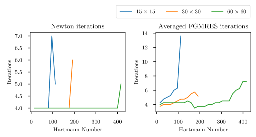
Figure 2: Number of Newton steps (left) and average number of iterations of preconditioned FGMRES using coupled Vanka to solve each linearization (right) when using continuation to solve the Hartmann problem with $Re=Re_{m}=H\!a$ on the $480\times 480$ mesh, with coarsest grids in the hierarchy of $15\times 15$, $30\times 30$, and $60\times 60$.

4.2 Two-dimensional island coalescence

We next consider a time-
dependent two-dimensional test problem that mimics magnetic reconnection in a large aspect ratio tokamak [10, 57]. In this setting, we consider the cross-section of flow of a magnetically confined plasma, in which a large magnetic field is imposed in the toroidal direction, resulting in effectively two-dimensional dynamics. We then consider an annulus in the cross-sectional direction that is unfolded and rescaled to make a square domain, $\Omega=[-1,1]^{2}$, with a periodic mapping between its right and left edges, see Figure 3.

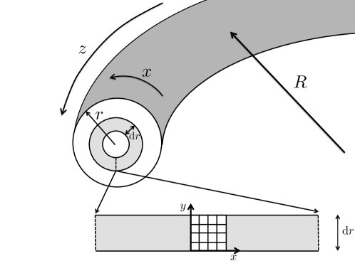
Figure 3: Cross-sectional view of large aspect-ratio tokamak geometry, with major radius, $R$, and minor radius, $r$, satisfying $R\gg r$. A cross-section of thickness d$r$ can be unfolded to create a Cartesian grid as pictured.

On this domain, we consider a model problem of a physical instability that can arise from perturbations of the magnetic current density, known as island coalescence, which has been simulated in numerous works (eg. [16, 14, 29, 15, 43, 3]). In this problem, two initially isolated “islands” of current density are perturbed, resulting in a breaking and then reconnection of the magnetic field lines. At the reconnection point, where the magnetic field comes back together, a sharp peak in current density occurs.

As an equilibrium solution, we take

$$\mathbf{u}_{0}(x,y) =\mathbf{0},$$

$$\mathbf{B}_{0}(x,y) =\frac{1}{\cosh(2\pi y)+k\cos(2\pi x)}\left(\begin{array}[]{c}\sinh(2\pi y)\\ k\sin(2\pi x)\end{array}\right),$$

$$p(x,y) =\frac{1-k^{2}}{2}\left(1+\frac{1}{\left(\cosh(2\pi y)+k\cos(2\pi x)\right)^{2}}\right),$$

$$r(x,y) =0,$$

for $k=0.2$. To support this as an equilibrium solution of Equations (1)–(4) requires imposition of right-hand side functions $\mathbf{f}=\mathbf{0}$ and

$$\mathbf{g}=\frac{-8\pi^{2}(k^{2}-1)}{Re_{m}\left(\cosh(2\pi y)+k\cos(2\pi x)\right)^{3}}\left(\begin{array}[]{c}\sinh(2\pi y)\\ k\sin(2\pi x)\end{array}\right).$$

As an initial condition, we perturb the equilibrium solution for the magnetic field by

$$\delta\mathbf{B}=\frac{\epsilon}{\pi}\left(\begin{array}[]{c}-\cos(\pi x)\sin(\pi y/2)\\ \cos(\pi y/2)\sin(\pi x)/2\end{array}\right),$$

taking $\epsilon=-0.01$. We measure physical fidelity of the simulation by considering the reconnection rate of the simulation, which is the time rate of change of the poloidal flux function, $\Psi$, such that $\mathbf{B}=-\nabla\times\left(0,0,\Psi\right)^{\top}$. In our formulation, this can be computed as the difference between $\nabla\times\mathbf{B}$ at the reconnection point (origin for our computational domain) at the current time to its initial value, scaled by $1/\sqrt{Re_{m}}$. For more details, see [10, 57]. For low magnetic Reynolds numbers, the area of reconnection is wider with a less steep gradient in the current density when the peak occurs. As the magnetic Reynolds number increases, this reconnection zone narrows, resulting in a sharper, yet shorter, peak. In addition, a “sloshing” effect occurs, where the islands bounce a little before fully merging into one [29]. This yields a peak in the reconnection rate, whose height oscillates as the islands come together. More sloshing occurs for higher magnetic Reynolds numbers. This is validated in our computational tests shown in Figure 4.

While the curl of a Nédélec field is naturally computed in a discontinuous Galerkin space (via the usual exact sequence), because we are interested in a pointwise measurement of the quantity, we instead project $\nabla\times\mathbf{B}$ onto the continuous space of piecewise linear functions for this measurement. This requires a solve with the mass matrix for the piecewise linear space, which we do using a simple multigrid method as a preconditioner for the conjugate gradient iteration. The preconditioner is formed once before time-stepping begins, and reused in a postprocessing step after each time step. We do not time this postprocessing step in the results below, so we have not made significant effort to optimize this computation. Since symmetry around the origin is important in this measurement, we discretize this problem on “crossed” triangular meshes, taking uniform quadrilateral meshes of $[-1,1]^{2}$ and cutting each square cell into 4 triangles, adding a vertex at the cell midpoint.

We discretize the temporal derivatives using the L-stable BDF2 method. For each spatial mesh, a fixed time-step is used; however, to start the time-stepping, a refinement of the first time-step into ten (equal) substeps is used, as we observed nonlinear convergence issues without this. For the first substep, a Crank-Nicolson discretization is used (to avoid the need for additional initial data for BDF2). There are two relevant CFL numbers for these simulations. The classical fluid CFL, which we take to be $u_{\text{max}}\frac{\Delta t}{h}$, where $u_{\text{max}}$ is the maximum magnitude of the velocity vector, $\mathbf{u}$, at a given time step, $\Delta t$ is the time step itself, and $h$ is the spatial mesh width, calculated as the length of the shortest edges of the crossed triangular mesh. Similarly, we consider the Alfvén CFL, defined as $B_{\text{max}}\frac{\Delta t}{h}$, where $B_{\text{m}ax}$ is the maximum magnitude of the magnetic field, $\mathbf{B}$. For these calculations, we approximate $u_{\text{max}}$ and $B_{\text{max}}$ by projecting $\mathbf{u}\cdot\mathbf{u}$ and $\mathbf{B}\cdot\mathbf{B}$ onto the scalar piecewise-constant space and taking the square root of the maximum elementwise value of that projection.

We consider this problem with $Re=Re_{m}$ values of 5,000, 10,000, and 20,000, on four levels of spatial refinement, from $320\times 320$ quadrilateral elements, each cut into 4 triangles in the “crossed” mesh, up to $2560\times 2560$ cut quadrilateral elements. For the finest mesh, the discretization leads to a discrete system with about 170 million degrees of freedom. For all meshes, we consider a multigrid hierarchy formed from a coarsest grid of size $20\times 20$. As we use a second-order time-stepping scheme, we consider a time-step of $\Delta t=0.025$ on the coarsest level, and halve the time-step with each (uniform) refinement of the spatial mesh. Figure 4 shows the reconnection rates for these problems, computed across the meshes. For the $Re_{m}=5,000$ case, we see that the reconnection rate is close to convergence already on the coarsest mesh, but that finer meshes are needed to accurately resolve the true dynamics at higher $Re_{m}$ values. For runs with $Re_{m}=40000$ (not shown here), convergence of the reconnection rate was not yet observed by the $2560\times 2560$ mesh. Additionally, we see the expected qualitative behavior: a reduction in reconnection rate and increase in “sloshing” with $Re_{m}$.

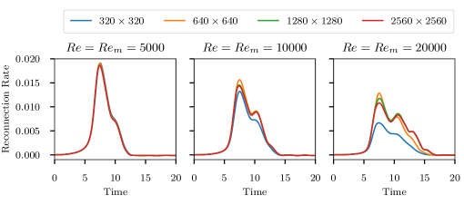
Figure 4: Reconnection rates computed for island coalescence model with $Re=Re_{m}$ values of 5,000 (left), 10,000 (middle), and 20,000 (right).

Figure 5 shows the number of linear iterations needed per time-step for these simulations, again only considering the coupled Vanka relaxation scheme. Here, based on preliminary experiments, we used V(3,3) multigrid cycles with the Chebyshev interval chosen to be $[2.0,10.0]$. For each time-step, we use the solution from the previous time-step as the initial guess for Newton’s method applied to the discretized nonlinear equations at the new time-step. Convergence is measured by requiring the $\ell_{2}$ norm of the nonlinear residual be reduced by either a relative factor of $10^{8}$ or to an absolute value below $10^{-6}$. Since time-stepping provides a good-quality initial guess, we observe that we typically require only one or two Newton steps to achieve convergence based on the absolute residual-norm tolerance. For coarser meshes, we observe some growth in the required number of linear iterations per time step as we increase $Re_{m}$, but this is largely mitigated on the finest meshes, where only a single linear iteration is needed per time step throughout the simulation. We note that the time steps used are chosen so that the Alfvén CFL number is larger than one (except in the first time step, where sub-steps are used to initialize the simulation), and kept at a constant factor of about 6 over all simulations, as shown in Figure 6. The fluid CFL is much more variable, peaking at values around 2 at the point where peak reconnection is observed. We note that the discretization has no stabilization to cope with the advective terms, and that problems with nonlinear solver convergence arose when simulations (not shown here) were run with higher fluid CFL values, as might be expected.

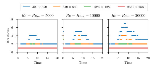
Figure 5: Number of linear solver iterations needed per time-step for island coalescence model with $Re=Re_{m}$ values of 5,000 (left), 10,000 (middle), and 20,000 (right).

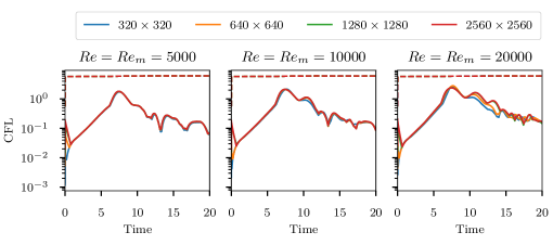
Figure 6: Measured CFL values at each time-step for island coalescence model with $Re=Re_{m}$ values of 5,000 (left), 10,000 (middle), and 20,000 (right). Solid lines denote the fluid CFL, dashed lines denote the Alfvén CFL.

A standard weak scaling experiment was performed. The simulations on the $320\times 320$ mesh were run on 10 cores of a single node on Niagara, requiring roughly 30GB of total memory and between 2 and 2.5 hours of wall-clock runtime, including initialization, input/output, and some postprocessing (such as computing the CFL values at each time-step, as shown above). With each refinement, the number of cores allotted was increased by a factor of four, leading to 40 cores (1 node) for the $640\times 640$ mesh, 160 cores (4 nodes) for the $1280\times 1280$ mesh, and 640 nodes (16 cores) for the $2560\times 2560$ mesh. Reported memory usage for all of these simulations peaks at about 110GB of memory per node. Figure 7 shows wall-clock runtimes for the nonlinear system solve at each timestep (including the linear system solve(s) required). Comparing with Figure 5, we see that the time per time step scales roughly with the number of linear iterations (as expected), and that there is not undue growth with problem size. Thus, the total wall-clock runtimes for these simulations grows roughly by a factor of 2 per refinement, due to the doubling of the number of time steps with each mesh refinement.

With such low iteration counts, a natural question to ask is whether or not the problem could be efficiently solved using a simpler preconditioner. To test this hypothesis, we considered the same simulations using just the multigrid relaxation scheme as the preconditioner, with no coarse-grid correction. On the $640\times 640$ mesh, at $Re_{m}=20000$, the initial timesteps require substantially more work, requiring up to 200 linear iterations per timestep, taking over 1 minute per timestep to compute, again on 40 cores. After some “spinup” time, the simulation becomes less expensive, still requiring about 40 linear iterations per timestep, costing about 0.3 seconds per timestep, around three times the cost per timestep of the multigrid simulation. Similar results were seen at lower Reynolds numbers, although somewhat mitigated, for example requiring 25-30 linear iterations per timestep at $Re_{m}=5000$, but still with a cost above double that of the multigrid simulation. While these results improve somewhat with mesh refinement, the need for and value of the coarse-grid correction process are clear.

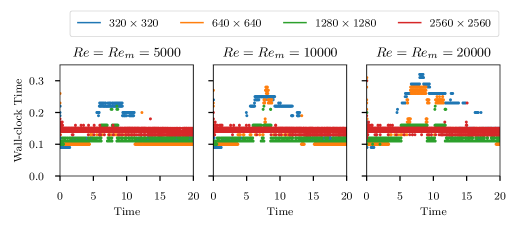
Figure 7: Wall-clock solution time needed per time-step for island coalescence model with $Re=Re_{m}$ values of 5,000 (left), 10,000 (middle), and 20,000 (right).

4.3 MHD Generator

Finally, we consider a three-dimensional steady-state test problem, where a duct flow is used to generate an electric current. Similar simulations have been considered in [55, 45, 62]. We use similar problem specifications as in [62], considering the domain $[0,5]\times[0,1]\times[0,1]$. For the velocity, we impose an inflow Dirichlet boundary condition of $\mathbf{u}=(1,0,0)^{\top}$ on the face with $x=0$, a natural boundary condition on the face with $x=5$, and no-slip boundary conditions of $\mathbf{u}=(0,0,0)^{\top}$ on the four other faces of the domain. On the “bottom” and “top” faces of the domain (with $z=0$ and $z=1$), we impose a Dirichlet boundary condition on the tangential component of $\mathbf{B}$, that is $\mathbf{n}\times\mathbf{B}=\mathbf{n}\times(0,b_{y}(x),0)^{\top}$ for outward unit normal vector $\mathbf{n}$, and

$$b_{y}(x)=\frac{B_{0}}{2}\left(\tanh\left(\frac{x-x_{\rm on}}{\delta}\right)-\tanh\left(\frac{x-x_{\rm off}}{\delta}\right)\right),$$

where $B_{0}=1$, $\delta=0.1$, $x_{\rm on}=2.0$, and $x_{\rm off}=2.5$. We fix the values of both the pressure and the Lagrange multiplier to be zero at the origin but, otherwise, impose no boundary conditions on these. For these simulations, we fix $Re=Re_{m}=H\!a=10$, as in the experiments of [62].

Table 3 presents linear and nonlinear convergence results for the test problem at 3 different levels of resolution using the coupled Vanka relaxation scheme. For this example, we use V(2,2) multigrid cycles with the Chebyshev relaxation interval chosen to be $[2.25,18.0]$. These meshes are created by constructing the coarsest mesh in the multigrid hierarchy, first as a mesh of hexahedra then “cutting” each hexahedron into six tetrahedra in the usual manner. These coarsest meshes are then refined uniformly as needed to generate the finest meshes in the hierarchy. Thus, the 2-level solver for the smallest problem size, the 3-level solver for the middle problem size, and the 4-level solver for the largest problem size all use the same coarsest mesh, starting from a $20\times 4\times 4$ mesh of hexahedra on the domain $[0,5]\times[0,1]\times[0,1]$ and refining one to three times. A consequence of this is that the different multigrid solvers for the same finest-grid problem sizes are solving slightly different problems, as the processes of cutting hexahedra into tetrahedra and regular refinement do not perfectly commute for these meshes. Nonetheless, we believe these problems present a fair comparison of the solver performance as we add levels to the multigrid hierarchies. For the nonlinear solver, we again use Newton’s method with Eisenstat-Walker for the stopping criteria. As expected, we see that the performance of Newton’s method is largely insensitive to the details of the linear solver. For both of the largest two problem sizes, we see some notable degradation in multigrid solver performance with the 4-level hierarchies, which we again ascribe to the poor resolution of this problem on the coarsest meshes of the hierarchy. For the middle problem size with the 4-level hierarchy, the underlying hexahedral cells are cubes with sidelength of $0.5$, while they are cubes of sidelength $0.25$ for the 4-level hierarchy and the largest problem size. In both cases, these significantly under-resolve the Reynolds numbers, so it is unsurprising that solver performance is compromised, particularly for a discretization without additional stabilization terms.

Table 3: Nonlinear and linear solver performance for MHD generator example. Problems with 724K DoFs were run on 5 cores, those with 5.6M DoFs were run on 40 cores (1 node), and those with 44M DoFs were run on 400 cores (10 nodes).

Finest grid size	724,725		5,600,229			44,023,749
Number of levels	2	3	2	3	4	3	4
Newton Steps	5	5	4	4	5	4	4
Total Linear iterations	52	62	42	44	117	58	184
Solution Time (minutes)	4.12	4.31	5.09	5.18	9.86	5.68	12.85

For the smallest problems, memory usage peaked at approximately 4 GB per core (20GB total), which rose slightly for the middle problem sizes, which required approximately 170 GB total, filling the available memory on one node of Niagara (after accounting for required system overhead). For the finest problem size, there was insufficient memory per node to run the solvers on 8 nodes, so these results were run on 10 nodes, requiring about 160 GB/node for the 4-level solver (with increased memory costs due to GMRES storage for the large iteration counts) and 153 GB/node for the 3-level solver. Solution times scale relatively clearly with linear iteration counts, leading to roughly scalable 3-level solvers (although we note the finest grid results clearly benefit in this comparison from the added CPUs available on 10 nodes). Finally, we note that it was not possible to test a “deeper” multigrid hierarchy on the finest mesh, due to a software requirement that there be at least one element per MPI thread on the coarsest mesh of the hierarchy. The coarsest mesh for the smaller problem sizes contains 240 elements (a $10\times 2\times 2$ hexahedral mesh refined into tetrahedra), which does not satisfy this constraint.

5 Conclusions

We present a monolithic multigrid preconditioner for the linearization of a mixed finite element discretization of the equations of viscoresistive incompressible MHD. A distinctive feature of this formulation is the presence of two Lagrange multipliers, one to enforce the incompressibility of fluid velocity, and one to enforce a similar divergence-free constraint on the magnetic field. Three variants of Vanka relaxation are considered; while the segregated approach breaks down when coupling between the fluid velocity and magnetic field is significant, both the purist and coupled approaches appear to provide robust solvers, with the coupled approach offering the most efficient performance. The associated multigrid solver is effective for the stationary and transient cases up to 170 million degrees of freedom.

The clear limitation of the approach presented here is the low order and lack of stabilization for the finite element discretization considered, and extending this to a better finite element discretization is the main focus for future work. We note the preconditioners proposed in [45, 55] are applied to stabilized finite element discretizations similar to those considered here, while excellent augmented Lagrangian preconditioners are developed for stabilized discretizations of the Navier–Stokes at large Reynolds numbers in [21, 20]. Another clear avenue for future work is the development of similar monolithic multigrid approaches for more detailed models of plasma, such as those considered in [56, 33, 37, 38, 46].

References

- [1] M. F. Adams, R. Samtaney, and A. Brandt, Toward textbook multigrid efficiency for fully implicit resistive magnetohydrodynamics, Journal of Computational Physics, 229 (2010), pp. 6208 – 6219.
- [2] J. H. Adler, T. R. Benson, E. Cyr, S. P. MacLachlan, and R. S. Tuminaro, Monolithic multigrid methods for two-dimensional resistive magnetohydrodynamics, SIAM Journal on Scientific Computing, 38 (2016), pp. B1–B24.
- [3] J. H. Adler, M. Brezina, T. A. Manteuffel, S. F. McCormick, J. W. Ruge, and L. Tang, Island coalescence using parallel first-order system least squares on incompressible resistive magnetohydrodynamics, SIAM Journal on Scientific Computing, 35 (2013), pp. S171–S191.
- [4] J. H. Adler, Y. He, X. Hu, and S. P. MacLachlan, Vector-potential finite-element formulations for two-dimensional resistive magnetohydrodynamics, Computers & Mathematics with Applications, 77 (2019), pp. 476–493.
- [5] J. H. Adler, T. A. Manteuffel, S. F. McCormick, J. W. Ruge, and G. D. Sanders, Nested iteration and first-order system least squares for incompressible, resistive magnetohydrodynamics, SIAM Journal on Scientific Computing, 32 (2010), pp. 1506–1526.
- [6] P. R. Amestoy, I. S. Duff, J. Koster, and J.-Y. L’Excellent, A fully asynchronous multifrontal solver using distributed dynamic scheduling, SIAM Journal on Matrix Analysis and Applications, 23 (2001), pp. 15–41.
- [7] D. N. Arnold, R. S. Falk, and R. Winther, Multigrid in and , Numer. Math., 85 (2000), pp. 197–217.
- [8] S. Balay, S. Abhyankar, M. F. Adams, J. Brown, P. Brune, K. Buschelman, L. Dalcin, A. Dener, V. Eijkhout, W. D. Gropp, D. Karpeyev, D. Kaushik, M. G. Knepley, D. A. May, L. Curfman McInnes, R. Tran Mills, T. Munson, K. Rupp, P. Sanan, B. F. Smith, S. Zampini, H. Zhang, and H. Zhang, PETSc users manual, Tech. Report ANL-95/11 - Revision 3.12, Argonne National Laboratory, 2019.
- [9] S. Balay, K. Buschelman, W. D. Gropp, D. Kaushik, M. G. Knepley, L. Curfman McInnes, B. F. Smith, and H. Zhang, PETSc Web page, 2020. http://www.mcs.anl.gov/petsc.
- [10] G. Bateman, MHD Instabilities, The MIT Press, 1978.
- [11] M. Benzi, G. H. Golub, and J. Liesen, Numerical solution of saddle point problems, Acta Numer., 14 (2005), pp. 1–137.
- [12] A. Brandt, Multigrid techniques: 1984 guide with applications to fluid dynamics, GMD–Studien Nr. 85, Gesellschaft für Mathematik und Datenverarbeitung, St. Augustin, 1984.
- [13] A. Brandt and N. Dinar, Multigrid solutions to elliptic flow problems, in Numerical Methods for Partial Differential Equations, Seymour V. Parter, ed., Academic Press, New York, 1979, pp. 53–147.
- [14] L. Chacón, An optimal, parallel, fully implicit Newton–Krylov solver for three-dimensional viscoresistive magnetohydrodynamics, Physics of Plasmas, 15 (2008), p. 056103.
- [15] L. Chacon, D. A. Knoll, and J. M. Finn, An implicit, nonlinear reduced resistive MHD solver, J. Comput. Phys., 178 (2002), pp. 15–36.
- [16] E. Cyr, J. Shadid, R. Tuminaro, R. Pawlowski, and L. Chacón, A new approximate block factorization preconditioner for two-dimensional incompressible (reduced) resistive MHD, SIAM Journal on Scientific Computing, 35 (2013), pp. B701–B730.
- [17] S. C. Eisenstat and H. F. Walker, Choosing the forcing terms in an inexact Newton method, SIAM Journal on Scientific Computing, 17 (1996), pp. 16–32.
- [18] H. Elman, V. E. Howle, J. Shadid, R. Shuttleworth, and R. Tuminaro, A taxonomy and comparison of parallel block multi-level preconditioners for the incompressible Navier-Stokes equations, J. Comput. Phys., 227 (2008), pp. 1790–1808.
- [19] P. E. Farrell, M. G. Knepley, L. Mitchell, and F. Wechsung, PCPATCH: Software for the topological construction of multigrid relaxation methods., 2019. arXiv:1912.08516.
- [20] P. E. Farrell, L. Mitchell, L. R. Scott, and F. Wechsung, A Reynolds-robust preconditioner for the Reynolds-robust Scott-Vogelius discretization of the stationary incompressible Navier-Stokes equations, arXiv preprint arXiv:2004.09398, (2020).
- [21] P. E. Farrell, L. Mitchell, and F. Wechsung, An augmented Lagrangian preconditioner for the 3D stationary incompressible Navier-Stokes equations at high Reynolds number, arXiv preprint arXiv:1810.03315, (2018).
- [22] F. Gaspar, Y. Notay, C. Oosterlee, and C. Rodrigo, A simple and efficient segregated smoother for the discrete Stokes equations, SIAM Journal on Scientific Computing, 36 (2014), pp. A1187–A1206.
- [23] C. Greif, D. Li, D. Schötzau, and X. Wei, A mixed finite element method with exactly divergence-free velocities for incompressible magnetohydrodynamics, Computer Methods in Applied Mechanics and Engineering, 199 (2010), pp. 2840 – 2855.
- [24] C. Greif and D. Schötzau, Preconditioners for the discretized time-harmonic Maxwell equations in mixed form, Numer. Linear Algebra Appl., 14 (2007), pp. 281–297.
- [25] K. Hu, W. Qiu, and K. Shi, Convergence of a - based finite element method for MHD models on Lipschitz domains, Journal of Computational and Applied Mathematics, 368 (2020), p. 112477.
- [26] V. John and G. Matthies, Higher-order finite element discretizations in a benchmark problem for incompressible flows, International Journal for Numerical Methods in Fluids, 37 (2001), pp. 885–903.
- [27] V. John and L. Tobiska, Numerical performance of smoothers in coupled multigrid methods for the parallel solution of the incompressible Navier-Stokes equations, International Journal for Numerical Methods in Fluids, 33 (2000), pp. 453–473.
- [28] R. C. Kirby and L. Mitchell, Solver composition across the PDE/linear algebra barrier, SIAM Journal on Scientific Computing, 40 (2018), pp. C76–C98.
- [29] D. A. Knoll and L. Chacón, Coalescence of magnetic islands, sloshing, and the pressure problem, Physics of Plasmas, 13 (2006).
- [30] M. Lange, L. Mitchell, M. G. Knepley, and G. J. Gorman, Efficient mesh management in firedrake using PETSc DMPlex, SIAM Journal on Scientific Computing, 38 (2016), pp. S143–S155.
- [31] M. Larin and A. Reusken, A comparative study of efficient iterative solvers for generalized Stokes equations, Numerical Linear Algebra with Applications, 15 (2008), pp. 13 – 34.
- [32] L. Li and W. Zheng, A robust solver for the finite element approximation of stationary incompressible MHD equations in 3D, J. Comput. Phys., 351 (2017), pp. 254–270.
- [33] J. Loverich, A. Hakim, and U. Shumlak, A discontinuous galerkin method for ideal two-fluid plasma equations, Communications in Computational Physics, 9 (2011), pp. 240–268.
- [34] Y. Ma, K. Hu, X. Hu, and J. Xu, Robust preconditioners for incompressible MHD models, Journal of Computational Physics, 316 (2016), pp. 721 – 746.
- [35] S. P. MacLachlan and C. W. Oosterlee, Local Fourier analysis for multigrid with overlapping smoothers applied to systems of PDEs, Numerical Linear Algebra with Applications, 18 (2011), pp. 751–774.
- [36] S. Manservisi, Numerical analysis of Vanka-type solvers for steady Stokes and Navier-Stokes flows, SIAM J. Numer. Anal., 44 (2006), pp. 2025–2056.
- [37] E. T. Meier and U. Shumlak, A general nonlinear fluid model for reacting plasma-neutral mixtures, Physics of Plasmas, 19 (2012), p. 072508.
- [38] S. T. Miller, E. C. Cyr, J. N. Shadid, R. M. J. Kramer, E. G. Phillips, S. Conde, and R. P. Pawlowski, Imex and exact sequence discretization of the multi-fluid plasma model, Journal of Computational Physics, 397 (2019), p. 108806.
- [39] M. F. Murphy, G. H. Golub, and A. J. Wathen, A note on preconditioning for indefinite linear systems, SIAM Journal on Scientific Computing, 21 (2000), pp. 1969–1972.
- [40] J.-C. Nédélec, Mixed finite elements in , Numer. Math., 35 (1980), pp. 315–341.
- [41] C. W. Oosterlee and F. J. Gaspar, Multigrid relaxation methods for systems of saddle point type, Applied Numerical Mathematics, 58 (2008), pp. 1933 – 1950.
- [42] B. Philip, L. Chacón, and M. Pernice, Implicit adaptive mesh refinement for 2D reduced resistive magnetohydrodynamics, Journal of Computational Physics, 227 (2008), pp. 8855 – 8874.
- [43] B. Philip, L. Chacón, and M. Pernice, Implicit adaptive mesh refinement for 2D reduced resistive magnetohydrodynamics, J. Comput. Phys., 227 (2008), pp. 8855–8874.
- [44] E. G. Phillips, H. C. Elman, E. C. Cyr, J. N. Shadid, and R. P. Pawlowski, A block preconditioner for an exact penalty formulation for stationary MHD, SIAM Journal on Scientific Computing, 36 (2014), pp. B930–B951.
- [45] E. G. Phillips, J. N. Shadid, E. C. Cyr, H. C. Elman, and R. P. Pawlowski, Block preconditioners for stable mixed nodal and edge finite element representations of incompressible resistive MHD, SIAM J. Sci. Comput., 38 (2016), pp. B1009–B1031.
- [46] E. G. Phillips, J. N. Shadid, E. C. Cyr, and S. T. Miller, Enabling scalable multifluid plasma simulations through block preconditioning, in Numerical Methods for Flows, Springer, 2020, pp. 231–244.
- [47] F. Rathgeber, D. A. Ham, L. Mitchell, M. Lange, F. Luporini, A. T. T. Mcrae, G.-T. Bercea, G. R. Markall, and P. H. J. Kelly, Firedrake: Automating the finite element method by composing abstractions, ACM Trans. Math. Softw., 43 (2016), pp. 24:1–24:27.
- [48] C. Rodrigo, F. J. Gaspar, and F. J. Lisbona, On a local Fourier analysis for overlapping block smoothers on triangular grids, Appl. Numer. Math., 105 (2016), pp. 96–111.
- [49] Y. Saad, Iterative methods for sparse linear systems, Society for Industrial and Applied Mathematics, Philadelphia, PA, second ed., 2003.
- [50] Y. Saad and M. H. Schultz, GMRES: A generalized minimal residual algorithm for solving nonsymmetric linear systems, SIAM Journal on Scientific and Statistical Computing, 7 (1986), pp. 856–869.
- [51] A. Schneebeli and D. Schötzau, Mixed finite elements for incompressible magneto-hydrodynamics, Comptes Rendus Mathematique, 337 (2003), pp. 71 – 74.
- [52] J. Schöberl and W. Zulehner, On Schwarz-type smoothers for saddle point problems, Numer. Math., 95 (2003), pp. 377–399.
- [53] D. Schötzau, Mixed finite element methods for stationary incompressible magneto–hydrodynamics, Numerische Mathematik, 96 (2004), pp. 771–800.
- [54] J. N. Shadid, R. P. Pawlowski, J. W. Banks, L. Chacón, P. T. Lin, and R. S. Tuminaro, Towards a scalable fully-implicit fully-coupled resistive MHD formulation with stabilized FE methods, Journal of Computational Physics, 229 (2010), pp. 7649 – 7671.
- [55] J. N. Shadid, R. P. Pawlowski, E. C. Cyr, R. S. Tuminaro, L. Chacón, and P. D. Weber, Scalable implicit incompressible resistive MHD with stabilized FE and fully-coupled Newton–Krylov-AMG, Computer Methods in Applied Mechanics and Engineering, 304 (2016), pp. 1–25.
- [56] B. Srinivasan and U. Shumlak, Analytical and computational study of the ideal full two-fluid plasma model and asymptotic approximations for hall-magnetohydrodynamics, Physics of Plasmas, 18 (2011), p. 092113.
- [57] H. R. Strauss, Nonlinear, Three-Dimensional Magnetohydrodynamics of Noncircular Tokamaks, Physics of Fluids, 19 (1976), pp. 134–140.
- [58] M. ur Rehman, T. Geenen, C. Vuik, G. Segal, and S. P. MacLachlan, On iterative methods for the incompressible Stokes problem, International Journal for Numerical Methods in Fluids, 65 (2011), pp. 1180–1200.
- [59] S. P. Vanka, Block-implicit multigrid calculation of two-dimensional recirculating flows, Computer Methods in Applied Mechanics and Engineering, 59 (1986), pp. 29 – 48.
- [60] , Block-implicit multigrid solution of Navier-Stokes equations in primitive variables, Journal of Computational Physics, 65 (1986), pp. 138 – 158.
- [61] R. Verfürth, A combined conjugate gradient - multi-grid algorithm for the numerical solution of the Stokes problem, IMA Journal of Numerical Analysis, 4 (1984), pp. 441–455.
- [62] M. Wathen and C. Greif, A scalable approximate inverse block preconditioner for an incompressible magnetohydrodynamics model problem, SIAM J. Sci. Comput., 42 (2020), pp. B57–B79.
- [63] M. Wathen, C. Greif, and D. Schötzau, Preconditioners for mixed finite element discretizations of incompressible MHD equations, SIAM J. Sci. Comput., 39 (2017), pp. A2993–A3013.
- [64] H. Wobker and S. Turek, Numerical studies of Vanka-type smoothers in computational solid mechanics, Adv. Appl. Math. Mech., 1 (2009), pp. 29–55.
- [65] Software used in ’Monolithic multigrid for magnetohydrodynamics’, June 2020. https://doi.org/10.5281/zenodo.3903199.