Global optimization using mixed integer quadratic programming on non-convex two-way interaction truncated linear multivariate adaptive regression splines

Abstract

Multivariate adaptive regression splines (MARS) is a flexible statistical modeling method that has been popular for data mining applications. MARS has also been employed to approxmiate unknown relationships in optimzation for complex systems, including surrogate optimization, dynamic programming, and two-stage stochastic programming. Given the increasing desire to optimize real world systems, this paper presents an approach to globally optimize a MARS model that allows up to two-way interaction terms that are products of truncated linear univariate functions (TITL-MARS). Specifally, such a MARS model consists of linear and quadratic structure. This structure is exploited to formulate a mixed integer quadratic programming problem (TITL-MARS-OPT). To appreciate the contribution of TITL-MARS-OPT, one must recognize that popular heurstic optimization approaches, such as evolutionary algorithms, do not guarantee global optimality and can be computationally slow. The use of MARS maintains the flexibility of modeling within TITL-MARS-OPT while also taking advantage of the linear modeling structure of MARS to enable global optimality. Computational results compare TITL-MARS-OPT with a genetic algorithm for two types of cases. First, a wind farm power distribution case study is described and then other TITL-MARS forms are tested. The results show the superiority of TITL-MARS-OPT over the genetic algorithm in both accuracy and computational time.

Keywords Multivariate adaptive regression splines (MARS) $\cdot$ Two-way interactions  $\cdot$ Quadratic optimization  $\cdot$ Mixed integer linear programminge

1 Introduction

Optimization for complex systems often involves fitting a system prediction model to estimate how a system performs and then optimizing the decisions based on the system prediction model as shown in Figure 1. Two major tasks in optimization of complex systems include training or meta-modeling a statistical or system model and optimizing input or decisions based on statistical model.

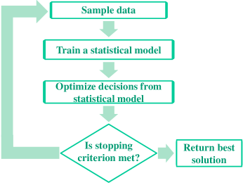
Figure 1: Optimization of complex systems

In real world complex systems, underlying relationships are commonly unknown and are approximated from data using empirical models. Wu et al. [1] applied support vector regression in travel time prediction and proved support vector regression was applicable in traffic data analysis. [2] applied a deep learning approach with autoencoders in traffic flow prediction. [3] used logistic regression to generate a landslide-hazard map to predict landslide hazards. [4] used multivariate adaptive regression splines to predict the distributions of freshwater diadromous fish.

If one seeks to optimize a complex system, the optimization method would need to be able to handle the data-driven approximation models. Given the wide range of possible approximation models, such as machine learning algorithms, the most commonly employed optimization approach in these situations is a heuristic approach, such as an evolutionary algorithm, that cannot guarantee global optimality. Rather than having the approximation model dictate the need for a heuristic optimization method, the research in this paper seeks a balance that utilizes a flexible approximation model with structure that can be exploited to enable true global optimization. In other words, the “best of both worlds” is sought, by achieving global optimality while still maintaining a flexible approximation model. The approxmation model of choice in this paper is multivariate adaptive regression splines (MARS), introduced by machine learning pioneer Jerome Friedman in 1991 [5]. The structure of MARS is based on a linear statistical spline model and provides a flexible fit to data while also achieving a parsimonious model.

The desire to conduct global optimization is seen in many applications, and there are a number of approaches classified as global optimization methods [6]. The primary challenge in achieving global optimality is that many real world applications involve multiple local optima. Finding a global optimum requires sifting through the local optima and recognizing when one is suboptimal. The vast majority of applications employ heuristic search algorithms seek to overcome the challenge of local optima, but do not guarantee global optimality. Examples include heuristics based on evolutionary algorithms [7, 8, 9], particle swarm optimization [10], the grasshopper optimization method [11], and the weighted superposition attraction method [12]. In order to guarantee global optimality, the approach in this paper takes advantage of well-known properties of mixed integer and quadratic programming (MIQP) [13].

Some recent applications in which MARS has been employed for empirical modeling include a water pollution prediction problem [14], the head load in a building [15], the estimation of landfill leachate [16], and the damage identification for web core composite bridges [17], In optimization problems, MARS has been employed as the empirical model to approximate unknown relationships in a variety of applications. For stochastic dynamic programming, the use of MARS to approximate the value function was introduced by [18]. Since then, the MARS value function approximation approach has been used to numerically solve a 30-dimensional water reservoir management problem [19], a 20-dimensional wastewater treatment system [20, 21, 22], and a 524-dimensional nonstationary ground-level ozone pollution control problem [23]. In revenue management, MARS was employed to estimate upper and lower bounds for the value function of a Markov decision problem [24, 25], and MARS was used to represent the revenue function in airline overbooking optimization [26]. In two-stage stochastic programming, MARS was used to efficiently represent the expected profit function for an airline fleet assignment problem [27]. This fleet assignment research was extended to utilize a cutting plane method with MARS to conduct the optimization [28].

The contribution of this current work extends the approach of [29], who developed a piece-wise linear MARS structure and formulated a mixed integer and linear programming problem to globally optimize vehicle design parameters to improve performance in crash simulations. The piece-wise linear MARS function may be nonconvex, and the approach of Martinez et al. will yield a global optimum. However, restricting to piece-wise linear forms limits the flexibility of the empirical model. Hence, in the current work, the MARS form employed is based on the original MARS model. The primary challenge for an optimization method is handling the nonconvex MARS interaction terms, which are products of univariate terms. By restricting to two-way interactions, we can utilize quadratic programming methods. In real world applications, two-way interactions are commonly sufficient for empirical modeling [30]

In summary, the contribution of the presented approach is a MIQP global optimization method for a MARS model that allows up to two-way interaction terms that are products of truncated linear univariate functions (TITL-MARS). This approach is referred to as TITL-MARS-OPT and is compared against a genetic algorithm for two types of cases. First, a wind farm power distribution case study is described, and then other TITL-MARS forms are tested. Python code for TITL-MARS and TITL-MARS-OPT will be made available on GitHub upon acceptance of this paper (https://github.com/JuXinglong/TITL-MARS-OPT).

The rest of this paper is organized as follows. Section 2 describes background on TITL-MARS. Section 3 presents the MIQP formulation for TITL-MARS-OPT. The computational study is given in Section 4, and Section 5 concludes the paper.

2 Background of two-way interaction truncated linear multivariate adaptive regression splines

This section introduces the two-way interaction truncated linear MARS (TITL-MARS) model. The two-way interaction truncated linear MARS regression model with the response variable ${f}(\mathbf{x}_{i})$ is to be built on the independent variable $\mathbf{x}_{i}$ and can be written in the form of the linear combination of the basis functions as [5]

$$\begin{array}[]{l}\hat{f}(\mathbf{x})=a_{0}+\sum_{m=1}^{M}\left\{a_{m}\cdot B_{m}(\mathbf{x})\right\}.\end{array}$$ (1)

The MARS model is denoted as $\hat{f}(\mathbf{x})$, and $a_{0}$ is the constant term of the model. The basis function is denoted as $B_{m}(\mathbf{x})$, and $a_{m}$ is the coefficient of $B_{m}(\mathbf{x})$. The index of the basis function is denoted as $m$, and $M$ is the total number of basis functions. The basis function $B_{m}(\mathbf{x})$ using the truncated linear term has the following form

$$\begin{array}[]{l}B_{m}(\mathbf{x})=\prod_{k=1}^{Km}[s_{k,m}\cdot(x_{v(k,m)}-t_{v(k,m)})]_{+}.\end{array}$$ (2)

The truncated linear term is denoted as ${[s_{k,m}\cdot(x_{v(k,m)}-t_{v(k,m)})]}_{+}$, and the basis function $B_{m}(\mathbf{x})$ is the product of truncated linear terms. The index of the truncated linear term in $B_{m}(\mathbf{x})$ is denoted as $k$, and $K_{m}$ is the total number of truncated linear terms in $B_{m}(\mathbf{x})$. The sign of the truncated linear term is $s_{k,m}$, which can be $+1$ or $-1$. The $v$-th component of $\mathbf{x}$ is denoted as $x_{v(k,m)}$, and $t_{v(k,m)}$ is the corresponding knot value. TITL-MARS is the special case of MARS in which $K_{m}\leqslant 2$.

3 Formulation of two-way interaction truncated linear MARS using mixed integer quadratic programming

The general mixed integer quadratic programming problem [13] is given as

$$\begin{array}[]{ll}\min&\frac{1}{2}\textbf{z}^{T}\textbf{Q}\textbf{z}+\textbf{c}^{T}\textbf{z}\\ {s.t.}&\textbf{A}\textbf{z}=\textbf{b}\\ {}&\textbf{l}\leqslant\textbf{z}\leqslant\textbf{u}\\ {}&\textbf{z}\in\mathbb{R}^{P}\times\mathbb{Z}^{D-P},\\ \end{array}$$ (3)

while the two-way interaction truncated linear MARS is given in Section 2. In (3), the decision variable is z, and the quadratic coefficients matrix is Q. The coefficients of the linear terms in the objective funtion are in vector c. The linear constraints are denoated as $\textbf{A}\textbf{z}=\textbf{b}$. The lower bound and upper bound of z are l and u, respectively. The dimension of z is $D$. There are $P$ dimensions of real values, and $D-P$ dimensions of integers. Problem in the form 3 can be solved using the CPLEX solver.

The TITL-MARS optimization prolbem is given as follows.

$$\min\,\, \hat{f}(\mathbf{x})=a_{0}+\sum_{m=1}^{M}\left\{a_{m}\cdot B_{m}(\mathbf{x})\right\}$$ (4)

s.t. $$\textbf{l}\leqslant\textbf{x}\leqslant\textbf{u}$$ (5)

$$\textbf{x}\in\mathbb{R}^{P}\times\mathbb{Z}^{D-P}$$ (6)

$$B_{m}(\mathbf{x})=\prod_{k=1}^{Km}[s_{k,m}\cdot(x_{v(k,m)}-t_{v(k,m)})]_{+}$$ (7)

$${{[s_{k,m}\cdot(x_{v(k,m)}-t_{v(k,m)})]}_{+}}=\max\{s_{k,m}\cdot(x_{v(k,m)}-t_{v(k,m)}),0\}$$ (8)

The objective function (4) is the TITL-MARS model. The constraint set (5) is the boundary of $\mathbf{x}$. The constraint set (6) specifies the data types. Constraints (7) and (8) specify the basis functions and the truncated linear terms.

Let $\mathcal{M}$ denote an upper bound of $|x_{v(k,m)}-t_{v(k,m)}|$ and $|t_{v(k,m)}-x_{v(k,m)}|$. Let $y_{k,m}$ be an indicator variable for the nonnegativity of $s_{k,m}\cdot(x_{v(k,m)}-t_{v(k,m)})$, an let $\eta_{k,m}$ denote the univariate truncated linear function, given as

$$\eta_{k,m}=[s_{k,m}\cdot(x_{v(k,m)}-t_{v(k,m)})]_{+}=\max\{s_{k,m}\cdot(x_{v(k,m)}-t_{v(k,m)}),0\}.$$ (9)

Specifically, when $s_{k,m}\cdot(x_{v(k,m)}-t_{v(k,m)})\geqslant 0$, $y_{k,m}=1$ and $\eta_{k,m}=s_{k,m}\cdot(x_{v(k,m)}-t_{v(k,m)})$, otherwise $y_{k,m}=0$ and $\eta_{k,m}=0$.

The TITL-MARS optimization prolbem can be formulated into a general mixed integer quadratic programming problem as follows.

$$\min\,\, a_{0}+\sum_{m=1}^{M}\left\{a_{m}\cdot\prod_{k=1}^{Km}\eta_{k,m}\right\}$$ (10)

s.t. $$s_{k,m}\cdot(x_{v(k,m)}-t_{v(k,m)})\leqslant\eta_{k,m}\leqslant s_{k,m}\cdot(x_{v(k,m)}-t_{v(k,m)})+\mathcal{M}\cdot(1-y_{k,m}),$$ (11)

$$\forall k=1,\ldots,K_{m},\forall m=1,\ldots,M$$

$$0\leqslant\eta_{k,m}\leqslant\mathcal{M}\cdot y_{k,m},\forall k=1,\ldots,K_{m},\forall m=1,\ldots,M$$ (12)

$$\textbf{l}\leqslant\textbf{x}\leqslant\textbf{u}$$ (13)

$$\textbf{x}\in\mathbb{R}^{P}\times\mathbb{Z}^{D-P}$$ (14)

$$\eta_{k,m}\in\mathbb{R},\forall k=1,\ldots,K_{m},\forall m=1,\ldots,M$$ (15)

$$y_{k,m}\in\mathbb{B},\forall k=1,\ldots,K_{m},\forall m=1,\ldots,M.$$ (16)

The objective (10) is the TITL-MARS model. Equations (11) - (16) formulate the basis functions into linear constraints and specifying the boundaries and data types.

TITL-MARS-OPT is an optimization process as shown in Figure 2. The process has two steps. The first step is to fit TITL-MARS model, and the second step optimizes TITL-MARS model using MIQP. The benefits of the optimization process has two aspects. First, TITL-MARS can be fit using most commercial MARS software. Second, MIQP can be globally optimized using CPLEX [31].

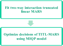
Figure 2: TITL-MARS-OPT optimization process

4 Experiments and results

In this section, first the genetic algorithm for TITL-MARS optimization is given, and then the presented TITL-MARS-OPT is tested on wind farm power distribution TITL-MARS models and other mathematical models with the genetic algorithm (TITL-MARS-GA) as a benchmark.

4.1 Genetic algorithm

The genetic algorithm can also be used as an optimization method to optimize the function (TITL-MARS-GA), as given in Algorithm 1 [32], where the input is the two-way interaction MARS model and the maximum generation number $M_{\max}$, and the output is an optimum and an optimum value. In the “initialization” step (line 1 in Algorithm 1), we generate a population and code the individuals from the decimal form to the binary form. In the “fitness value” step (line 2), we decode the individuals from the binary form to the decimal form and evaluate each of the individual’s decimal values in the MARS model function to obtain the fitness value. In the “keep the best” step (line 3), we sort the individuals by their fitness values and store the individual with the best fitness value. The “selection” step (line 6) selects parents from the prior population. The “crossover” (line 7) chooses two parents and produces a new population. The “mutation” (line 8) chooses one point within an individual and changes it from 1 to 0 or from 0 to 1. In this paper, the TITL-MARS-GA algorithm is used as a benchmark compared with the TITL-MARS-OPT method.

Data: $\hat{f}(\mathbf{x})=a_{0}+\sum_{m=1}^{M}\left\{a_{m}\cdot\prod_{k=1}^{Km}[s_{k,m}\cdot(x_{v(k,m)}-t_{v(k,m)})]_{+}\right\},M_{\max}$

Result: $\mathbf{x}_{\max},f(\mathbf{x}_{\max})$

1 Initialization: Generate a population and code the individuals from decimal to binary.

2 Fitness value: Decode individuals from binary to decimal and get function value.

3 Keep the best: Store the individual with highest or lowest fitness value.

4 $\mbox{gen}=1$

5 while gen$<M_{\max}$ do

6       Selection: Select parents from prior population.

7       Crossover: Choose two parents and produce a new population.

8       Mutation: Choose one point and $1\rightarrow 0$ or $0\rightarrow 1$.

9       Fitness value: Decode individuals from binary to decimal and get function value.

10       Keep the best: Store the individual with highest or lowest fitness value.

11       $\mbox{gen}=\mbox{gen}+1$

12 end while

Algorithm 1 Genetic algorithm for TITL-MARS optimization

The parameters of TITL-MARS-GA in this paper are from the literatures [33] and [32], and given in Table 1.

Table 1: Parameter settings of TITL-MARS-GA

Parameter	[33]	[32]
Population size	30	50
Maximum number of generations	300	1000
Crossover rate	0.9	0.8
Mutation rate	0.01	0.15

The TITL-MARS-GA optimization process has two steps as shown in Figure 3. The first step fits a two-way interaction truncated linear MARS model, and the second step optimizes decisions of TITL-MARS using the genetic algorithm. The drawback of TITL-MARS-GA is that it does not guarantee global optimality.

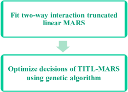
Figure 3: TITL-MARS-GA optimization process

4.2 Experimental environment

The experiments are run on a workstation with 64 bit Windows 10 Enterprise system. The CPU version is an Intel(R) CPU E3-1285 v6 @ 4.10GHz, and the RAM has 32 GB.The programming code is written in Python version is 3.6, and the CPLEX solver version is 12.8.

4.3 Optimization of wind farm power distribution function

Wind farm power is of paramount significance as a renewable energy source. In this paper, the Monte Carlo method [34] is used to generate random wind farm layouts, and the TITL-MARS method is used to study the power distribution under certain wind speeds and directions. After the TITL-MARS model is generated, the TITL-MARS-OPT method is used to study the best turbine position and the worst position. We use the following steps to generate the wind farm power distribution function, as shown in Figure 4. First, we randomly generate $N$ wind farm layouts. Second, we calculate average power output at each location. Third, we use the data from second step to build the TITL-MARS power distribution model.

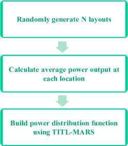
Figure 4: Steps to generate a TITL-MARS wind farm power distribution model

After the wind passes through a wind turbine $j$, a part of the wind energy will be absorbed by turbine $j$ and leave the downstream wind with the reduced speed, which is called the wake effect [35], and the wake effect model is shown in Figure 5.

(a) Wind wake effect model

(b) Wake effect illustration

Figure 5: Wake effect

Wind speed at turbine $i$ with the wake effect of turbine $j$ is $v_{i,j}$ and can be calculated as

$$v_{i,j}=v_{0}\left(1-\frac{2}{3}\cdot\frac{R_{j}^{2}}{r_{j}^{2}}\right).$$ (17)

$R_{j}$ is the radius of the wind turbine $j$, and $r_{j}$ is the wake radius of the wind turbine $j$. The final wind speed $v_{i}$ at turbine $i$ with multiple wake effects is given as

$$\begin{array}[]{l}v_{i}=v_{0}\left[1-\sqrt{\sum\limits_{j\in\Phi_{i}}\left(1-\frac{v_{i,j}}{v_{0}}\right)^{2}}\right],\end{array}$$ (18)

where $\Phi_{i}$ is the index set of the turbines which are upwind of the turbine $i$. Afterwards, the actual power of turbine $i$ can be obtained as [36]

$$p(v_{i})=\left\{{\begin{array}[]{*{20}{ll}}{0,}&v_{i}<2\\ {0.3{v_{i}}^{3},}&{2\leqslant v_{i}<12.8}}{\\ {629.1,}&12.8{\mkern 1.0mu}\leqslant{v_{i}\leqslant 18}\\ {0,}&v_{i}>18{\mkern 1.0mu},\\ \end{array}}\right.$$ (19)

and the power curve is shown in Figure 6. which is the relationship between the wind turbine power and the wind speed.

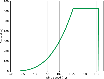
Figure 6: Relationship of wind speed with output power of a wind turbine

The wind farm power distribution is generated using the Monte Carlo methods for a given wind farm and a specific wind distribution.

$f_{w1}$ is generated from a wind farm where there is only one wind speed and one direction. The wind farm is divided into 41 by 41 cells, and each cell has a width of 308 m. The wind is from northeast ($\frac{\pi}{4}$) at 15 m/s.

$f_{w2}$ is generated from a wind farm where the wind has only one wind speed and four directions. The wind farm has the same dimension as that of $f_{w1}$. The wind is from north (0), south ($\pi$), east ($\frac{\pi}{2}$), and west ($\frac{3\pi}{2}$) at 15 m/s.

$f_{w3}$ is generated from a wind farm where the wind has only one wind speed at 15 m/s and six directions, 0, $\frac{\pi}{3}$, $\frac{2\pi}{3}$, $\pi$, $\frac{4\pi}{3}$, and $\frac{5\pi}{3}$.

$f_{w4}$ is generated from a wind farm where the wind has three wind speeds, 12 m/s, 10 m/s, and 8 m/s, and 12 directions, 0, $\frac{\pi}{6}$, $\frac{\pi}{3}$, $\frac{\pi}{2}$, $\frac{2\pi}{3}$, $\pi$, $\frac{7\pi}{6}$, $\frac{4\pi}{3}$, $\frac{3\pi}{2}$, $\frac{5\pi}{3}$, and $\frac{11\pi}{6}$.

TITL-MARS-OPT and TITL-MARS-GA are used to optimize on the wind farm power distribution models to find a global maximum and a minimum, and the results are shown in Figure 7 and summarized in Table 2. The results are the average value of 30 executions. The table shows the optimal values derived from the TITL-MARS-OPT and TITL-MARS-GA, as well as the computation time in seconds. The result shows that the TITL-MARS-OPT method finds better solutions than the genetic algorithm and uses less time. The maximum value and minimum value are very useful before actually building the wind turbines. The maximum location indicates that it is the best location to build a wind turbine based on the given requirements. The minimum location indicates that this location is the worst location on the wind farm, and if the budget is tight, the piece of land around the minimum location can be neglected.

Table 2: Comparison of TITL-MARS-OPT and TITL-MARS-GA on wind farm power distribution TITL-MARS models

Function	Measurement	MARS-OPT	MARS-GA 1	MARS-GA 2	MARS-GD
$f_{w1}$	Maximum	636.76	618.40	630.75	608.50
	Time(seconds)	0.15	1.45	9.06	0.04
	Minimum	578.30	579.18	578.33	579.21
	Time(seconds)	0.32	1.46	9.08	0.04
$f_{w2}$	Maximum	588.10	569.96	585.42	582.50
	Time(seconds)	0.15	1.46	9.18	0.04
	Minimum	545.90	545.88	545.85	545.91
	Time(seconds)	0.40	1.48	9.15	0.08
$f_{w3}$	Maximum	622.10	608.13	621.48	609.20
	Time(seconds)	0.15	1.49	9.36	0.08
	Minimum	599.50	599.77	599.51	599.86
	Time(seconds)	0.85	1.52	9.34	0.05
$f_{w4}$	Maximum	393.80	387.92	393.13	382.71
	Time(seconds)	0.04	1.57	9.72	0.23
	Minimum	303.21	303.46	303.21	303.91
	Time(seconds)	0.51	1.58	9.67	0.01

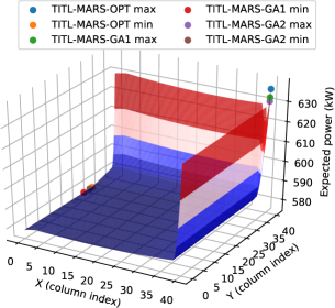
(a) Case 1 : $f_{w1}$

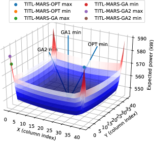
(b) Case 2 : $f_{w2}$

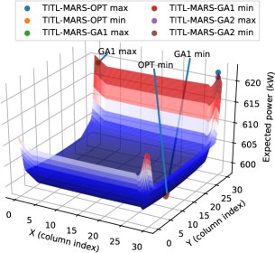
(c) Case 3 : $f_{w3}$

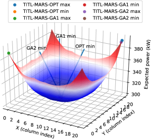
(d) Case 4 : $f_{w4}$

Figure 7: One run result comparison of TITL-MARS-OPT and TITL-MARS-GA on wind farm power distribution TITL-MARS model

4.4 Optimization of other functions

TITL-MARS-OPT method and TITL-MARS-GA are tested to optimize other six TITL-MARS models to find the global maximum and minimum. The first two TITL-MARS models $f_{1}$ and $f_{2}$ are two-dimensional [37]. The $f_{3}$ and $f_{4}$ are 10-dimensional TITL-MARS models. $f_{5}$ is 19-dimensional, and $f_{6}$ is 21-dimensional [38]. The results are shown in Figure 11 and summarized in Table 3. The results are the average value of 30 runs and show TITL-MARS-OPT is superior to TITL-MARS-GA. The result shows that TITL-MARS-OPT achieves better solutions than TITL-MARS-GA and uses less time, which is consistent with the prior result. The results also show that TITL-MARS-OPT is robust in dealing both low-dimensional and high-dimensional TITL-MARS models.

Table 3: Result comparison of TITL-MARS-OPT and TITL-MARS-GA on six other TITL-MARS mathematical models

Function	Measurement	MARS-OPT	MARS-GA 1	MARS-GA 2	MARS-GD
$f_{1}$	Maximum	8.30	6.23	8.27	6.60
	Time(seconds)	0.70	1.50	9.25	2.38
	Minimum	-8.20	-6.42	-6.33	-5.06
	Time(seconds)	1.65	1.51	9.18	0.57
$f_{2}$	Maximum	1.81	1.02	1.45	1.24
	Time(seconds)	0.31	1.42	8.91	1.71
	Minimum	-2.20	-1.38	-2.20	-1.38
	Time(seconds)	0.32	1.42	8.88	1.54
$f_{3}$	Maximum	5,774.08	5,092.52	5,410.16	5661.76
	Time(seconds)	0.02	2.71	15.74	0.02
	Minimum	-1126.39	2,289.47	903.69	-806.86
	Time(seconds)	0.02	2.67	15.81	10.35
$f_{4}$	Maximum	48,800.26	-13,516.73	-19,762.80	-1,891,678.92
	Time(seconds)	96.32	2.98	17.67	14.24
	Minimum	-3,952,146.24	-2,605,904.95	-3,599,093.85	-3,119,142.40
	Time(seconds)	0.41	2.95	17.57	0.01
$f_{5}$	Maximum	97,679.99	78,263.13	92,458.62	80,461.36
	Time(seconds)	0.02	5.20	30.01	28.45
	Minimum	-15,439.62	33,298.80	5,904.35	719.07
	Time(seconds)	2.46	5.21	30.38	28.72
$f_{6}$	Maximum	111,225.22	63,506.19	105,645.30	88956.05
	Time(seconds)	0.02	5.34	30.62	29.90
	Minimum	-14,215.61	17,886.61	494.43	-5757.07
	Time(seconds)	0.04	5.33	30.58	12.64

Table 4: Result comparison of true function value

Function	Measurement	OPT function(model)	MARS+GD	GA 1	GA 2	GD	PL-OPT	PL OPT+GD
$f_{1}$	Maximum	8.01(8.32)	8.21	8.20	8.21	5.76	-4.76(-5.15)	2.96
	Time(seconds)	0.25	0.24	0.78	7.58	0.01	0.05	0.00
	Minimum	-4.56(-8.16)	-6.20	-3.75	-5.76	-3.30	-4.86(-5.58)	-6.20
	Time(seconds)	10.57	0.73	0.77	7.54	0.01	0.05	0.00
$f_{2}$	Maximum	0.86(1.81)	1.00	1.00	1.00	1.00	0.31(0.56)	1.00
	Time(seconds)	0.10	0.14	0.59	5.25	0.10	0.24	0.00
	Minimum	-0.61(-2.20)	-1.00	-0.87	-1.00	-0.96	-0.46(-0.53)	-1.00
	Time(seconds)	2.65	0.22	0.54	5.27	0.10	0.13	0.00
$f_{3}$	Maximum	6,029.13(5,774.08)	6132.00	5,488.40	5,647.09	5893.00	4821.00(4667.86)	6132.00
	Time(seconds)	0.01	0.01	1.90	18.81	0.01	0.07	0.00
	Minimum	-826.08(-1,126.39)	-923.86	2,755.59	742.00	-525.09	288.27(118.11)	-123.44
	Time(seconds)	0.01	0.01	1.85	18.81	0.47	0.05	0.00
$f_{4}$	Maximum	-1,991.28(48,800.26)	-0.01	-1,643,753.96	-131,067.27	-0.01	-505,071.14(-398,359.99)	-0.01
	Time(seconds)	107.47	112.74	2.12	21.98	2.47	0.07	0.00
	Minimum	-4,581,942.36(-3,952,146.24)	-4,616,810.03	-3,651,963.86	-3,834,009.84	-3,161,354.60	-4,433,291.39(-3,945,225.00)	-4,616,810.03
	Time(seconds)	0.40	0.42	2.04	21.83	0.01	0.10	0.00

(a) $f_{1}$

(b) $f_{2}$

(c) $f_{3}$

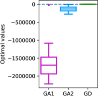
(d) $f_{4}$

Figure 8: maximum values boxplot

(a) $f_{1}$

(b) $f_{2}$

(c) $f_{3}$

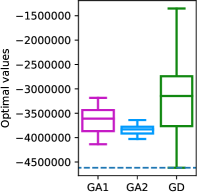
(d) $f_{4}$

Figure 9: minimum values boxplot

4.5 $f_{1}$, $f_{2}$, $f_{3}$ and $f_{4}$ functions

$$f_{1}({x_{1},x_{2}})= 3(1-x_{1})^{2}\exp(-x_{1}^{2}-(x_{2}+1)^{2})-10(\frac{x_{1}}{5}-x_{1}^{3}-x_{2}^{5})\exp(-x_{1}^{2}-x_{2}^{2})$$ (20)

$$-\frac{1}{3}\exp(-(x_{1}+1)^{2}-x_{2}^{2})+2x_{1},$$

$$-2\leqslant x_{1}\leqslant 2,-2\leqslant x_{2}\leqslant 2$$

$$f_{2}(x_{1},x_{2})= \sin\left(\frac{\pi x_{1}}{12}\right)\cos\left(\frac{\pi x_{2}}{16}\right)$$ (21)

$$-20\leqslant x_{1}\leqslant 20,-20\leqslant x_{2}\leqslant 20$$

$$f_{3}(\mathbf{x})= x_{1}^{2}+x_{2}^{2}+x_{1}x_{2}-14x_{1}-16x_{2}+(x_{3}-10)^{2}-4(x_{4}-5)^{2}+(x_{5}-3)^{2}$$ (22)

$$+2(x_{6}-1)^{2}+5x_{7}^{2}+7(x_{8}-11)^{2}+2(x_{9}-10)^{2}+2(x_{10}-7)^{2}+45$$

$$-10\leqslant x_{i}\leqslant 10$$

$$f_{4}(\mathbf{x})= \sum\limits_{j=1}^{10}\exp(x_{j})\left(c_{j}+x_{j}-\ln\sum\limits_{k=1}^{10}\exp(x_{k})\right)$$ (23)

$$\mathbf{c}=[-0.6089,-17.164,-34.054,-5.914,-24.721,-14.986,-24.100,-10.708,$$

$$-26.662,-22.179]$$

$$-10\leqslant x_{i}\leqslant 10$$

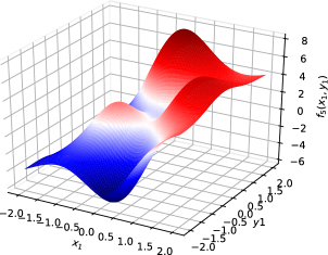
(a) $f_{1}(x_{1},x_{2})$

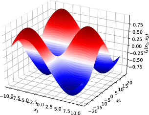
(b) $f_{2}(x_{1},x_{2})$

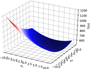
(c) $f_{3}(x_{1},x_{2})\mbox{ other }x_{i}=4.0$

(d) $f_{4}(x_{1},x_{2})\mbox{ other }x_{i}=3.0$

Figure 10: Surfaces of dataset functions

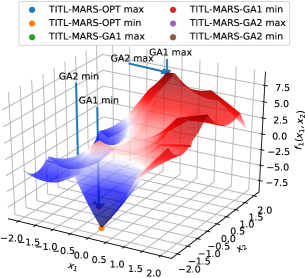
(a) $f_{1}$

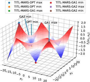
(b) $f_{2}$

Figure 11: One run result comparison of TITL-MARS-OPT and TITL-MARS-GA on $f_{1}$ and $f_{2}$ TITL-MARS models

5 Conclusion

In this paper, a new method (TITL-MARS-OPT) is proposed to globally optimize analytically on the two-way interaction truncated linear MARS (TITL-MARS) by using mixed integer quadratic programming. We verified the presented TITL-MARS-OPT method on the wind farm power distribution TITL-MARS models and six other mathematical TITL-MARS models. The application on wind farm power distribution models gives the best location and worst location information on the wind farm. The testing TITL-MARS models are from 2-dimensions to up to 21-dimensions, and it shows the TITL-MARS-OPT method is robust in dealing with TITL-MARS models with varied dimensions. We also compared the TITL-MARS-OPT method with TITL-MARS-GA in TITL-MARS model optimization, and it shows that the new method can achieve better accuracy and time efficiency. TITL-MARS-OPT can achieve as high as 316% and on average 46% better solution quality and is on average 175% faster than TITL-MARS-GA. In addition, the Python code and the testing models of this paper are made open source, and it will contribute to the study of TITL-MARS models and optimization.

Appendix A Supplemental materials

A.1 $f_{1}$, $f_{2}$, $f_{3}$ and $f_{4}$ functions

$$f_{1}({x_{1},x_{2}})= 3(1-x_{1})^{2}\exp(-x_{1}^{2}-(x_{2}+1)^{2})-10(\frac{x_{1}}{5}-x_{1}^{3}-x_{2}^{5})\exp(-x_{1}^{2}-x_{2}^{2})$$ (24)

$$-\frac{1}{3}\exp(-(x_{1}+1)^{2}-x_{2}^{2})+2x_{1},$$

$$-2\leqslant x_{1}\leqslant 2,-2\leqslant x_{2}\leqslant 2$$

$$f_{2}(x_{1},x_{2})= \sin\left(\frac{\pi x_{1}}{12}\right)\cos\left(\frac{\pi x_{2}}{16}\right)$$ (25)

$$-20\leqslant x_{1}\leqslant 20,-20\leqslant x_{2}\leqslant 20$$

$$f_{3}(\mathbf{x})= x_{1}^{2}+x_{2}^{2}+x_{1}x_{2}-14x_{1}-16x_{2}+(x_{3}-10)^{2}-4(x_{4}-5)^{2}+(x_{5}-3)^{2}$$ (26)

$$+2(x_{6}-1)^{2}+5x_{7}^{2}+7(x_{8}-11)^{2}+2(x_{9}-10)^{2}+2(x_{10}-7)^{2}+45$$

$$-10\leqslant x_{i}\leqslant 10$$

$$f_{4}(\mathbf{x})= \sum\limits_{j=1}^{10}\exp(x_{j})\left(c_{j}+x_{j}-\ln\sum\limits_{k=1}^{10}\exp(x_{k})\right)$$ (27)

$$\mathbf{c}=[-0.6089,-17.164,-34.054,-5.914,-24.721,-14.986,-24.100,-10.708,$$

$$-26.662,-22.179]$$

$$-10\leqslant x_{i}\leqslant 10$$

A.2 $f_{5}$ and $f_{6}$ functions

The datasets to generate $f_{5}$ and $f_{6}$ are from [38]. [38] applied adaptive dynamic programming for high-dimensional, multicollinear state sapce and used an Atlanta ozone pollution problem as the case study. The datasets used in this paper are from the fourth stage and the third stage with low variance inflation factors.

A.3 Details about transforming TITL-MARS into MIQP

The detailed steps of transforming TITL-MARS into MIQP are given in Algorithm 2. The objective function is the general form of MIQP given in (3). In step 1, let $\mathbf{x}$ be the $V$ dimensional decision variable of the original MARS model $\hat{f}(\mathbf{x})$. The step 4 defines $D$ as the dimension of the decision variable of the new MIQP problem. The step 6 defines $\mathbf{z}$ as the new decision variable of the objective function (3) where the first element is 1.0 for $a_{0}$ in the original problem. In step 7, let $\mathbf{c}$ be the coefficient vector for the linear elements in the new MIQP problem which is initialized to be a $\mathbf{0}$ vector. Steps 8 to 11 determine the values of $\mathbf{c}$. The coefficient for the first decision element 1.0 in $\mathbf{z}$ is $a_{0}$. For the univariate basis function $B_{m}(\mathbf{x})$, the corresponding element in the decision variable of MIQP is $\eta_{1,m}$ and the coefficient is $a_{m}$. Steps 12 to 17 define $\mathbf{Q}$ as the $D$ by $D$ coefficient matrix for the quadratic element in MIQP which is symmetric and is initialized to be $\mathbf{0}$. For the two-way interaction basis function $B_{m}(\mathbf{x})$, the corresponding coefficient in $Q$ matrix is $a_{m}$. Steps 18 to 31 transform the quadratic terms into linear constraints.

Data: $\hat{f}(\mathbf{x})=a_{0}+\sum_{m=1}^{M}\left\{a_{m}\cdot\prod_{k=1}^{Km}[s_{k,m}\cdot(x_{v(k,m)}-t_{v(k,m)})]_{+}\right\},K_{m}\leqslant 2,\,\mathcal{M}$

Result: $\hat{f}(\mathbf{z})=\frac{1}{2}\textbf{z}^{T}\textbf{Q}\textbf{z}+\textbf{c}^{T}\textbf{z}$

1 $\textbf{x}=(x_{1},x_{2},\dots x_{v},\dots x_{V}),\textbf{x}\in\mathbb{R}^{V}$

2 $\eta_{k,m}=[s_{k,m}\cdot(x_{v(k,m)}-t_{v(k,m)})]_{+},\,\eta_{k,m}\in\mathbb{R},\,\eta_{k,m}\geqslant 0$

3 $y_{k,m}=\left\{{\begin{array}[]{*{10}{ll}}{1}&s_{k,m}\cdot(x_{v(k,m)}-t_{v(k,m)})\geqslant 0\\ {0}&s_{k,m}\cdot(x_{v(k,m)}-t_{v(k,m)})<0\end{array}}\right.,y_{k,m}\in\mathbb{B}$

4 $D=1+V+\sum_{m=1}^{M-1}K_{m}$

5 $\textbf{z}\in\mathbb{R}^{D}$

6 $\textbf{z}=(1,x_{1},\dots,x_{V},\eta_{1,1},y_{1,1},\dots,\underbrace{\eta_{1,m-1},y_{1,m-1}}_{K_{m-1}=1},\underbrace{\eta_{1,m},y_{1,m},\eta_{2,m},y_{2,m}}_{K_{m}=2},\dots,\eta_{K_{{M-1},M-1}},y_{K_{{M-1},M-1}})$

7 $\textbf{c}=\textbf{0}\in\mathbb{R}^{D}$

8 $\textbf{c}_{0}=a_{0}$

9 for $m=1\,\mbox{to}\,M$ do

10      if $K_{m}=1$ then $\textbf{c}(\eta_{1,m})=a_{m}$;

11      

12 end for

13$\textbf{Q}=\textbf{0}\in\mathbb{R}_{D\times D}$

14 for $m=1\,\mbox{to}\,M$ do

15      if $K_{m}=2$ then

16            $\textbf{Q}(\eta_{1,m},\eta_{2,m})=a_{m},\,\,\textbf{Q}(\eta_{2,m},\eta_{1,m})=a_{m}$

17       end if

18      

19 end for

20for $m=1\,\mbox{to}\,M$ do

21      if $K_{m}=2\,\mbox{and}\,s_{k,m}=+1$ then

22            Add constraint: $x_{v(k,m)}-\eta_{k,m}-\mathcal{M}\cdot y_{k,m}\geqslant t_{v(k,m)}-\mathcal{M}$

23             Add constraint: $-x_{v(k,m)}+\eta_{k,m}\geqslant-t_{v(k,m)}$

24             Add constraint: $-\eta_{k,m}+\mathcal{M}\cdot y_{k,m}\geqslant 0$

25       end if

26      

27 end for

28for $m=1\,\mbox{to}\,M$ do

29      if $K_{m}=2\,\mbox{and}\,s_{k,m}=-1$ then

30            Add constraint: $-x_{v(k,m)}-\eta_{k,m}-\mathcal{M}\cdot y_{k,m}\geqslant-t_{v(k,m)}-\mathcal{M}$

31             Add constraint: $x_{v(k,m)}+\eta_{k,m}\geqslant t_{v(k,m)}$

32             Add constraint: $-\eta_{k,m}+\mathcal{M}\cdot y_{k,m}\geqslant 0$

33       end if

34      

35 end for

Algorithm 2 Formulation of two-way interaction truncated linear MARS into mixed integer quadratic programming

References

- Wu et al. [2004] Chun-Hsin Wu, Jan-Ming Ho, and Der-Tsai Lee. Travel-time prediction with support vector regression. IEEE transactions on intelligent transportation systems, 5(4):276–281, 2004.
- Lv et al. [2014] Yisheng Lv, Yanjie Duan, Wenwen Kang, Zhengxi Li, and Fei-Yue Wang. Traffic flow prediction with big data: a deep learning approach. IEEE Transactions on Intelligent Transportation Systems, 16(2):865–873, 2014.
- Ohlmacher and Davis [2003] Gregory C Ohlmacher and John C Davis. Using multiple logistic regression and gis technology to predict landslide hazard in northeast kansas, usa. Engineering geology, 69(3-4):331–343, 2003.
- Leathwick et al. [2005] JR Leathwick, D Rowe, J Richardson, Jane Elith, and T Hastie. Using multivariate adaptive regression splines to predict the distributions of new zealand’s freshwater diadromous fish. Freshwater Biology, 50(12):2034–2052, 2005.
- Friedman [1991] Jerome H Friedman. Multivariate adaptive regression splines. The annals of statistics, pages 1–67, 1991.
- Horst et al. [2000] Reiner Horst, Panos M Pardalos, and Nguyen Van Thoai. Introduction to global optimization. Springer Science & Business Media, 2000.
- Morra et al. [2018] Lia Morra, Nunzia Coccia, and Tania Cerquitelli. Optimization of computer aided detection systems: An evolutionary approach. Expert Systems With Applications, 100:145–156, 2018.
- Russo et al. [2018] Igor LS Russo, Heder S Bernardino, and Helio JC Barbosa. Knowledge discovery in multiobjective optimization problems in engineering via genetic programming. Expert Systems with Applications, 99:93–102, 2018.
- Dahi et al. [2018] Zakaria Abdelmoiz Dahi, Enrique Alba, and Amer Draa. A stop-and-start adaptive cellular genetic algorithm for mobility management of gsm-lte cellular network users. Expert Systems with Applications, 106:290–304, 2018.
- Alswaitti et al. [2018] Mohammed Alswaitti, Mohanad Albughdadi, and Nor Ashidi Mat Isa. Density-based particle swarm optimization algorithm for data clustering. Expert Systems with Applications, 91:170–186, 2018.
- Ewees et al. [2018] Ahmed A Ewees, Mohamed Abd Elaziz, and Essam H Houssein. Improved grasshopper optimization algorithm using opposition-based learning. Expert Systems with Applications, 112:156–172, 2018.
- Baykasoğlu and Ozsoydan [2018] Adil Baykasoğlu and Fehmi Burcin Ozsoydan. Dynamic optimization in binary search spaces via weighted superposition attraction algorithm. Expert Systems with Applications, 96:157–174, 2018.
- Bliek1ú et al. [2014] Christian Bliek1ú, Pierre Bonami, and Andrea Lodi. Solving mixed-integer quadratic programming problems with ibm-cplex: a progress report. In Proceedings of the twenty-sixth RAMP symposium, pages 16–17, 2014.
- Kisi and Parmar [2016] Ozgur Kisi and Kulwinder Singh Parmar. Application of least square support vector machine and multivariate adaptive regression spline models in long term prediction of river water pollution. Journal of Hydrology, 534:104–112, 2016.
- Roy et al. [2018] Sanjiban Sekhar Roy, Reetika Roy, and Valentina E Balas. Estimating heating load in buildings using multivariate adaptive regression splines, extreme learning machine, a hybrid model of mars and elm. Renewable and Sustainable Energy Reviews, 82:4256–4268, 2018.
- Bhatt et al. [2017] Arpita H Bhatt, Richa V Karanjekar, Said Altouqi, Melanie L Sattler, MD Sahadat Hossain, and Victoria P Chen. Estimating landfill leachate bod and cod based on rainfall, ambient temperature, and waste composition: Exploration of a mars statistical approach. Environmental Technology & Innovation, 8:1–16, 2017.
- Mukhopadhyay [2018] Tanmoy Mukhopadhyay. A multivariate adaptive regression splines based damage identification methodology for web core composite bridges including the effect of noise. Journal of Sandwich Structures & Materials, 20(7):885–903, 2018.
- Chen et al. [1999] Victoria CP Chen, David Ruppert, and Christine A Shoemaker. Applying experimental design and regression splines to high-dimensional continuous-state stochastic dynamic programming. Operations Research, 47(1):38–53, 1999.
- Cervellera et al. [2006] Cristiano Cervellera, Victoria CP Chen, and Aihong Wen. Optimization of a large-scale water reservoir network by stochastic dynamic programming with efficient state space discretization. European journal of operational research, 171(3):1139–1151, 2006.
- Tarun et al. [2011] Prashant K Tarun, Victoria CP Chen, HW Corley, and Feng Jiang. Optimizing selection of technologies in a multiple stage, multiple objective wastewater treatment system. Journal of Multi-Criteria Decision Analysis, 18(1-2):115–142, 2011.
- Tsai et al. [2004] Julia CC Tsai, Victoria CP Chen, M Bruce Beck, and Jining Chen. Stochastic dynamic programming formulation for a wastewater treatment decision-making framework. Annals of Operations Research, 132(1-4):207–221, 2004.
- Tsai and Chen [2005] Julia CC Tsai and Victoria CP Chen. Flexible and robust implementations of multivariate adaptive regression splines within a wastewater treatment stochastic dynamic program. Quality and Reliability Engineering International, 21(7):689–699, 2005.
- Yang et al. [2009] Zehua Yang, Victoria CP Chen, Michael E Chang, Melanie L Sattler, and Aihong Wen. A decision-making framework for ozone pollution control. Operations Research, 57(2):484–498, 2009.
- Chen et al. [2003] Victoria CP Chen, Dirk Günther, and Ellis L Johnson. Solving for an optimal airline yield management policy via statistical learning. Journal of the Royal Statistical Society: Series C (Applied Statistics), 52(1):19–30, 2003.
- Siddappa et al. [2007] Sheela Siddappa, Dirk Günther, Jay M Rosenberger, and Victoria CP Chen. Refined experimental design and regression splines method for network revenue management. Journal of Revenue and Pricing Management, 6(3):188–199, 2007.
- Siddappa et al. [2008] Sheela Siddappa, Jay M Rosenberger, and Victoria CP Chen. Optimising airline overbooking using a hybrid gradient approach and statistical modelling. Journal of Revenue and Pricing Management, 7(2):207–218, 2008.
- Pilla et al. [2008] Venkata L Pilla, Jay M Rosenberger, Victoria CP Chen, and Barry Smith. A statistical computer experiments approach to airline fleet assignment. IIE transactions, 40(5):524–537, 2008.
- Pilla et al. [2012] Venkata L Pilla, Jay M Rosenberger, Victoria Chen, Narakorn Engsuwan, and Sheela Siddappa. A multivariate adaptive regression splines cutting plane approach for solving a two-stage stochastic programming fleet assignment model. European Journal of Operational Research, 216(1):162–171, 2012.
- Martinez et al. [2017] Nadia Martinez, Hadis Anahideh, Jay M Rosenberger, Diana Martinez, Victoria CP Chen, and Bo Ping Wang. Global optimization of non-convex piecewise linear regression splines. Journal of Global Optimization, 68(3):563–586, 2017.
- Kutner et al. [2005] Michael H Kutner, Christopher J Nachtsheim, John Neter, William Li, et al. Applied linear statistical models, volume 5. McGraw-Hill Irwin Boston, 2005.
- ILOG [2018] IBM ILOG. Ibm ilog cplex optimization studio cplex user’s manual, 2018.
- Michalewicz [1996] Zbigniew Michalewicz. Evolution strategies and other methods. In Genetic Algorithms+ Data Structures= Evolution Programs, pages 159–177. Springer, 1996.
- Grefenstette [1986] John J Grefenstette. Optimization of control parameters for genetic algorithms. IEEE Transactions on systems, man, and cybernetics, 16(1):122–128, 1986.
- Metropolis and Ulam [1949] Nicholas Metropolis and Stanislaw Ulam. The monte carlo method. Journal of the American statistical association, 44(247):335–341, 1949.
- Jensen [1983] Niels Otto Jensen. A note on wind generator interaction. 1983.
- Liu and Wang [2013] Feng Liu and Zhifang Wang. Electric load forecasting using parallel rbf neural network. In Global Conference on Signal and Information Processing (GlobalSIP), 2013 IEEE, pages 531–534. IEEE, 2013.
- Miyata and Shen [2005] Satoshi Miyata and Xiaotong Shen. Free-knot splines and adaptive knot selection. Journal of the Japan Statistical Society, 35(2):303–324, 2005.
- Ariyajunya [2013] Bancha Ariyajunya. Adaptive dynamic programming for high-dimensional, multicollinear state spaces. 2013.