Intrinsic charm in the nucleon and charm production at large rapidities in collinear, hybrid and $k_{T}$-factorization approaches

Abstract

We discuss the role of intrinsic charm (IC) in the nucleon for forward production of $c$-quark (or $\bar{c}$-antiquark) in proton-proton collisions for low and high energies. The calculations are performed in collinear-factorization approach with on-shell partons, $k_{T}$-factorization approach with off-shell partons as well as in a hybrid approach using collinear charm distributions and unintegrated (transverse momentum dependent) gluon distributions. For the collinear-factorization approach we use matrix elements for both massless and massive charm quarks/antiquarks. The distributions in rapidity and transverse momentum of charm quark/antiquark are shown for a few different models of IC. Forward charm production is dominated by $gc$-fusion processes. The IC contribution dominates over the standard pQCD (extrinsic) $gg$-fusion mechanism of $c\bar{c}$-pair production at large rapidities or Feynman-$x_{F}$. We perform similar calculations within leading-order and next-to-leading order $k_{T}$-factorization approach. The $k_{T}$-factorization approach leads to much larger cross sections than the LO collinear approach. At high energies and large rapidities of $c$-quark or $\bar{c}$-antiquark one tests gluon distributions at extremely small $x$. The IC contribution has important consequences for high-energy neutrino production in the Ice-Cube experiment and can be, to some extent, tested at the LHC by the SHIP and FASER experiments by studies of the $\nu_{\tau}$ neutrino production.

I Introduction

The text-book proton consists of $uud$ valence quarks. This picture is by far too simplified. In fact there is strong evidence for internal strangeness and somewhat smaller for internal charm content of the nonperturbative proton. Different pictures of nonperturbative $c\bar{c}$ content were proposed in the past. A first example is relatively old BHPS model BHPS1980 which assumes $uudc\bar{c}$ 5-parton Fock configurations (see also Refs. BHK1982 ; VB1996 ). Another picture proposed in the literature is a meson cloud model (MCM) NNNT1996 ; MT1997 ; SMT1999 ; CDNN2001 ; HLM2014 , where the $p\to{\bar{D}}^{0}\Lambda_{c}$ or $D\Sigma_{c}$ fluctuations of the proton are considered. While in the first model $c(x)={\bar{c}}(x)$ in the MCM $c(x)\neq{\bar{c}}(x)$. The models do not allow to predict precisely the absolute probability for the $c$-quark or $\bar{c}$-antiquark content of the proton. Experimental data put only loose constraints on the charm content:

$$\int_{0}^{1}c(x)\;dx=\int_{0}^{1}{\bar{c}}(x)\;dx<0.01\;.$$ (1)

It is rather upper limit but this value depends somewhat on the model of charm content of a proton. In general, for sea-like models the probability can be slightly larger than for the BHPS one. In the sea-like case the charm is concentrated at lower values of $x$. Very recent lattice study of charm quark electromagnetic form factors suggested asymmetry of $c$-quark and $\bar{c}$-antiquark distributions latticeQCD .

Recently there is a renewed interest in the intrinsic charm (IC) which is related to experiments being performed at the LHC BBLS2015 ; RKAG2016 ; LLSB2016 ; BBLLMST2018 . The intrinsic charm is often included in global parton analyses of world experimental data BKLSSV2015 ; Ball:2014uwa ; Hou:2017khm .

The highly energetic neutrino experiments, such as IceCube, could put further constraints on the intrinsic charm ERS2008 ; LB2016 ; GGN2018 . Here, however, the IC contribution may compete with a concept of the subleading fragmentation Maciula:2017wov . Similarly, future LHC high and low energy forward experiments like FASER and SHIP could also be very helpful in this context (see e.g. Ref. Bai:2020ukz and Ref. Bai:2018xum , respectively). Also the LHCb experiment in its fixed-target mode could be sensitive to the contributions coming from intrinsic charm in a proton, especially in the case of open charm production Aaij:2018ogq , where some problems with a satisfactory theoretical description of the experimental data were reported (see also discussion in Ref. Maciula:2020cfy ).

In this paper we concentrate therefore on forward production of charm quarks/antiquarks. There were already some studies performed with color glass condensate approach and compared to the dipole approach at forward directions GNU2010 ; CGGN2017 . In our approach we will use instead collinear, hybrid and $k_{T}$-factorization approach. The latter two were not studied so far in the context of IC and forward production of charm.

II Models of intrinsic charm in a nucleon

In the five-quark Fock component $uudc\bar{c}$ heavy quark/antiquark carries rather large fraction of the mother proton. In the BHPS model, after some approximations the probability to find $c$ or $\bar{c}$ (the same for both) can be expressed via a simple formula:

$$\frac{dP}{dx}=c(x)={\bar{c}}(x)=Ax^{2}\left(6x(1+x)ln(x)+(1-x)(1+10x+x^{2})\right)\;.$$ (2)

The normalization constant $A$ depends on integrated probability for $c\bar{c}$ component and is 6 for 1 % probability. Please note that the quark mass is not explicit in this simplified formula.

In the meson cloud models $c$ is in the baryon-like object and $\bar{c}$ in the meson-like object. Then the probabilistic distribution can be obtained as

$$\frac{dP_{c}}{dx} = \int_{x}^{1}\frac{dy}{y}f_{B}(y)f_{c/B}(x/y)\;,$$ (3)

$$\frac{dP_{\bar{c}}}{dx} = \int_{x}^{1}\frac{dy}{y}f_{M}(y)f_{\bar{c}/M}(x/y)\;.$$ (4)

The $f_{B}$ and $f_{M}$ functions, the probability to find meson or baryon in proton, can be calculated from corresponding Lagrangians supplemented by a somewhat arbitrary and poorly known vertex form factors and can be found e.g. in Ref. HLM2014 . In general, such an approach leads to $c(x)\neq{\bar{c}}(x)$.

In practice both models give rather similar distributions as will be shown in the following, so using one of them as an example is representative and sufficient. These are models of large-$x$ components of IC. In principle, the IC may have also small-$x$ component known under the name of sea-like, however, only simple ad hoc parametrizations were used in the literature.

Figure 1: A dynamical process leading to sea-like IC.

There is another category of processes leading to sea-like IC (see Fig. 1 where an example of corresponding dynamical processes is shown). Using intrinsic glue in the nucleon (see e.g. Ref. EI1998 ) one can generate intrinsic charm sea. The intrinsic gluon distribution fulfil by construction the relation:

$$\int_{0}^{1}\left(xu_{v}(x)+xd_{v}(x)+xg(x)\right)dx=1\;.$$ (5)

For massless charm the intrinsic charm can be calculated as the convolution with initial (intrinsic) glue

$$c(x)={\bar{c}}(x)=\alpha_{s}(4m_{c}^{2})/(2\pi)\int_{x}^{1}dy\left(\frac{1}{y}\right)P_{qg}\left(\frac{x}{y}\right)g(y)\;,$$ (6)

where $g$ is the intrinsic gluon distribution. With the model from Ref. EI1998 the $c$ and $\bar{c}$ distributions are integrable, concentrated at $x\sim$ 0.1-0.2 and corresponding probability is 2.7 %. It should be less for massive quarks/antiquarks. In Fig. 2 we show $x$-distribution of the IC for the BHPS and for the sea-like model described above.

Figure 2: Charm quark/antiquark distribution for the two different models of IC. The solid line represents the BHPS model while the dashed line is for sea-like glue as obtained in a way described above. In this calculation BHPS model with 1% probability was used for illustration.

In the GRV approach Gluck:1994uf the charm contribution is calculated fully radiatively as the convolution of gluon distribution with appropriate mass-dependent splitting function:

$$xc(x,Q^{2})=\frac{\alpha_{s}(\mu^{\prime 2})}{2\pi}\int_{ax}^{1}dy\left(\frac{x}{y}\right)C_{g,2}^{c}\left(\frac{x}{y},\ \frac{m_{c}^{2}}{Q^{2}}\right)g(y,\mu^{\prime 2})\;.$$ (7)

The explicit formula for $C_{g,2}^{c}$ and $a$, including mass of quarks/antiquarks, can be found in Ref. Gluck:1994uf . In the following calculations we will use more modern gluon distributions.

In this paper we concentrate on large-$x$ component and completely ignore the sea-like component(s). Charm can also be generated by evolution equations via $g\to c\bar{c}$ transition (splitting). Often it was included in the evolution as a massless parton with zero as initial condition at the starting scale $\mu^{2}\sim m_{c}^{2}$. In a dedicated fits, the intrinsic charm distribution is used as initial condition for DGLAP evolved charm distributions (see e.g. Ref. PLT2007 ). In the right panel Fig. 4 we show charm distribution in a proton without (dashed line) and with (solid line) the IC distribution taken as initial condition of the evolution.

III Cross section for associated charm production

III.1 The collinear approach

In the present study we discuss production of the final states with one charm quark or charm antiquark. In the collinear approach Collins:1989gx the final state charm must be associated with at least one additional gluon or (light) quark. Typical leading-order mechanisms for charm production initiated by charm quark in a initial state are shown in Fig. 9. The diagrams correspond to the $gc\to gc$ (or $g\bar{c}\to g\bar{c}$) subprocesses that are expected to be dominant at high energies, however, the $qc\to qc$ and $\bar{q}c\to\bar{q}c$ (or $q\bar{c}\to q\bar{c}$ and $\bar{q}\bar{c}\to\bar{q}\bar{c}$) mechanisms with $q=u,d,s$ are also possible and will be taken into account in the following numerical calculations.

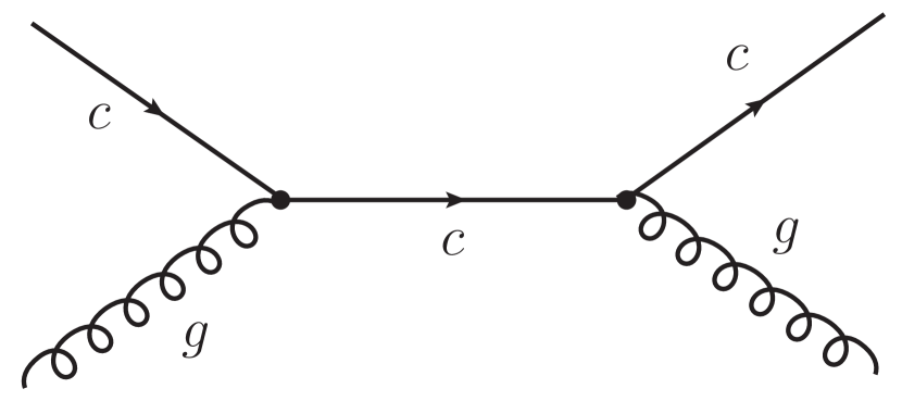
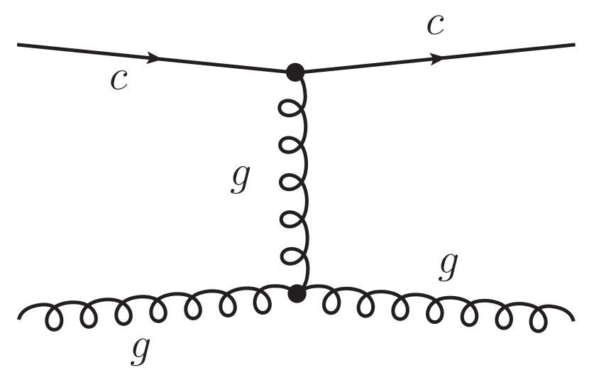
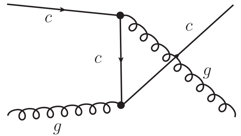
Figure 3: Typical leading-order (2 $\to$ 2) mechanisms of production of $c$ quarks or $\bar{c}$ antiquarks in the collinear parton model.

In the collinear approach the differential cross section for forward charm production within the $gc\to gc$ mechanism can be calculated as

$$\frac{d\sigma}{dy_{1}dy_{2}d^{2}p_{t}}=\frac{1}{16\pi{\hat{s}}^{2}}\overline{|{\cal M}_{gc\to gc}|^{2}}x_{1}g(x_{1},\mu^{2})x_{2}c(x_{2},\mu^{2})\;,$$ (8)

where ${\cal M}_{gc\to gc}$ is the on-shell matrix element for $gc\to gc$ subprocesses and $g(x_{1},\mu^{2})$ and $c(x_{2},\mu^{2})$ are the collinear gluon and charm quark PDFs evaluated at longitudinal momentum fractions $x$ and factorization scale $\mu^{2}$.

Including the mass of charm quark the on-shell matrix element takes the following form:

$$\overline{|{\cal M}_{gc\to gc}|^{2}} = g_{s}^{4}\left[\left(-m_{c}^{4}(3\hat{s}^{2}+14\hat{s}\hat{u}+3\hat{u}^{2})+m_{c}^{2}(\hat{s}^{3}+7\hat{s}^{2}\hat{u}+7\hat{s}\hat{u}^{2}+\hat{u}^{3})\right.\right.$$ (9)

$$\left.\left.+6m_{c}^{8}-\hat{s}\hat{u}(\hat{s}^{2}+\hat{u}^{2})\right)\left(-18m_{c}^{2}(\hat{s}+\hat{u})+18m_{c}^{4}+9\hat{s}^{2}+9\hat{u}^{2}-\hat{t}^{2}\right)\right]$$

$$/\left(18\hat{t}^{2}(\hat{u}-m_{c}^{2})^{2}(\hat{s}-m_{c}^{2})\right)^{2},$$

where $g_{s}^{2}=4\pi\alpha_{s}(\mu)$. In the massless limit $m_{c}\to 0$ one recovers the known textbook formula:

$$\overline{|{\cal M}_{gc\to gc}|^{2}}=g_{s}^{4}\left(-\frac{4}{9}\left(\frac{{\hat{u}}^{2}+{\hat{s}}^{2}}{{\hat{u}}{\hat{s}}}\right)+\left(\frac{{\hat{u}}^{2}+{\hat{s}}^{2}}{{\hat{t}}^{2}}\right)\right)\;.$$ (10)

A role of the charm quark mass in the matrix element will be discussed when presenting numerical results.

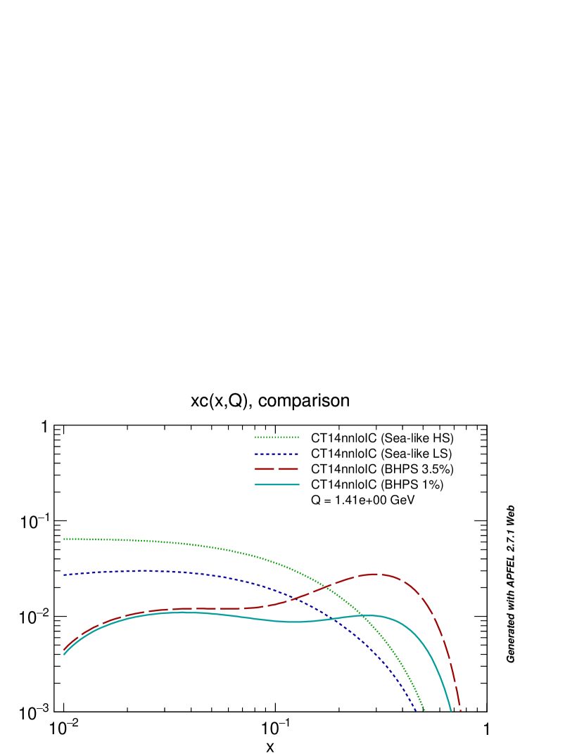
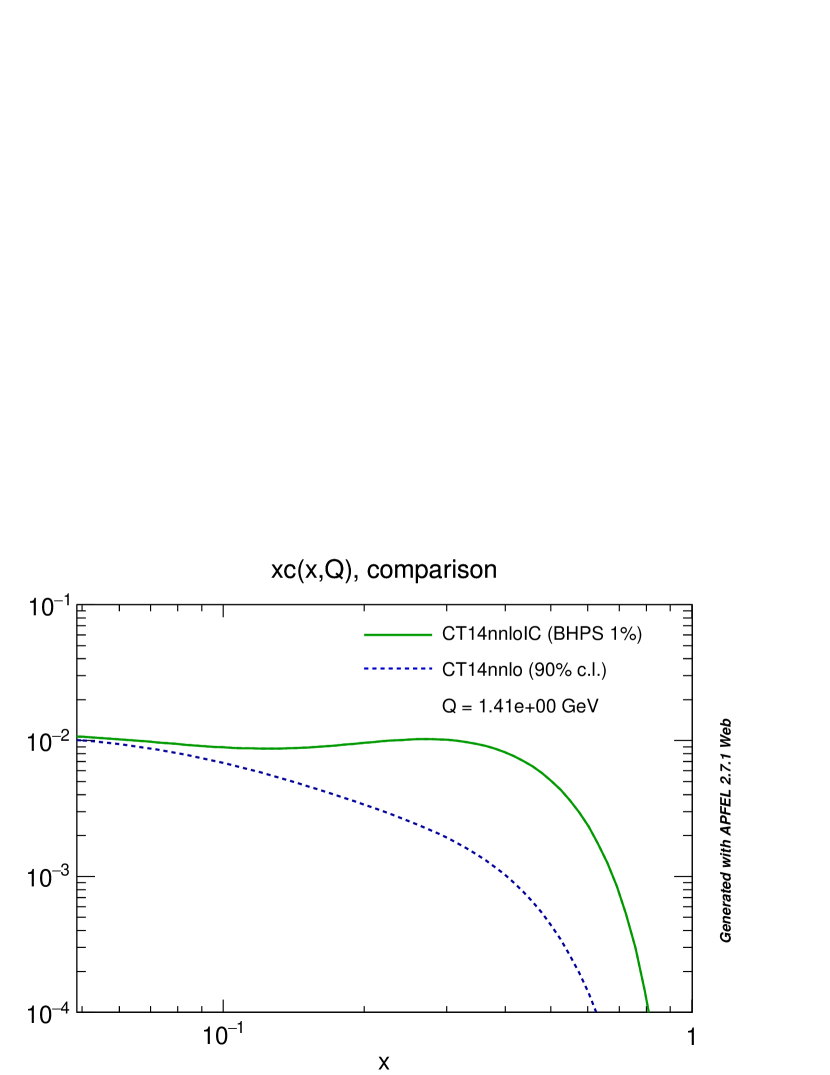
Figure 4: Charm quark distributions in a proton as a function of longitudinal momentum fraction $x$. Here different models for initial intrinsic charm quark distributions are shown (left panel) and a comparison between charm quark distributions obtained with and without concept of intrinsic charm in the proton.

In the numerical calculations below the intrinsic charm PDFs are taken at the initial scale $m_{c}=1.3$ GeV, so the perturbative charm contribution is intentionally not taken into account. We apply four different grids of the intrinsic charm distributions from the CT14nnloIC PDF Hou:2017khm that correspond to the BHPS 1% and BHPS 3.5% as well as the sea-like LS (low-strength) and sea-like HS (high-strength) models for initial intrinsic charm distribution. The distributions are compared with each other in the left panel of Fig. 4. In the right panel we present in addition the difference between the CT14nnloIC charm PDF obtained with and without intrinsic-charm concept.

On the other hand the collinear gluon PDFs $g(x,\mu^{2})$ are taken at the running factorization scale related to the averaged transverse momentum of the outgoing particles, i.e. $\mu=\sqrt{\frac{p_{t1}^{2}+p_{t2}^{2}}{2}+m_{c}^{2}}$. The charm quark mass $m_{c}=1.3$ GeV plays here a role of the minimal scale and ensures that we are not going beyond the fitted PDF grids where unconstrained extrapolation procedures are applied. We keep the charm quark mass here even when the massless matrix element and/or kinematics are used.

As will be shown later, the numerical results strongly depend on how the longitudinal momentum fractions $x_{1}$ and $x_{2}$ (arguments of parton distributions) are calculated. In the massive scheme of the calculations the quantities are defined as follows:

$$x_{1} = \frac{p_{t1}}{\sqrt{s}}\exp(+y_{1})+\frac{m_{t2}}{\sqrt{s}}\exp(+y_{2})\;,$$

$$x_{2} = \frac{p_{t1}}{\sqrt{s}}\exp(-y_{1})+\frac{m_{t2}}{\sqrt{s}}\exp(-y_{2})\;.$$ (11)

In this equations $p_{t1}$ is transverse momentum of the outgoing gluon (or light quark/antiquark) and the $m_{t2}$ is $c$ quark ($\bar{c}$ antiquark) transverse mass defined as $m_{t}=\sqrt{p_{t}^{2}+m_{c}^{2}}$. As will be discussed further it is crucial to include in kinematics the mass of the final charm, while the initial charm can be considered massless. In the following numerical studies all the calculations in the massless limit with massless matrix elements will be done within the kinematics corrected in the above manner. The effect of the correction will be also explicitly shown.

Considering forward production of charm at the LHC energies one is exploring asymmetric kinematical regions where $x_{1}$ is very small (down to $10^{-5}$) and $x_{2}$ is rather large (about $10^{-1}$). Thus in this reaction small-$x$ gluon PDF and intrinsic large-$x$ charm content of the proton are probed simultaneously. As it is shown in Fig. 5 both distributions are not well constrained by the global experimental data. In the left panel we show the central fits for intrinsic charm distribution from the CT14nnloIC and the NNPDF30nloIC PDF sets Ball:2016neh together with $1\sigma$ standard deviation. In the right panel we compare gluon PDF fits from different collaborations, including MMHT2014nlo Harland-Lang:2014zoa , JR14NLO08FF Jimenez-Delgado:2014twa and CT14lo/nnlo sets. Clearly the current level of knowledge of both distributions is rather limited and the large uncertainties prevent definite conclusions. In principle, a study of far-forward production of charm may improve the situation by exploring unconstrained areas.

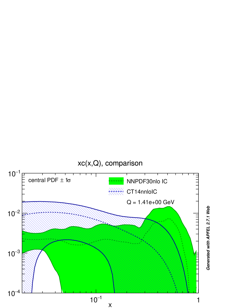
Figure 5: The intrinsic charm (left panel) and gluon (right panel) distributions in a proton as a function of longitudinal momentum fraction $x$. Here different sets of collinear PDFs are shown including uncertainties.

In the present study we go beyond the leading-order mechanisms and include also higher-order processes that are expected to play important role. We take into account all $2\to 3$ and $2\to 4$ processes at tree-level that lead to a production of charm quark or antiquark and are driven by the $gc$ and $qc$ (or $\bar{q}c$) initial state interactions. Examples of the diagrams corresponding to the processes are shown in Fig. 6. The relevant cross sections are calculated with the help of the KaTie Monte Carlo generator vanHameren:2016kkz .

Figure 6: Examples of the $2\to 3$ (left panel) and the $2\to 4$ (right panel) mechanisms of production of $c$ quarks or $\bar{c}$ antiquarks in the collinear parton model.

Having massless partons (minijets) in the final states considered in the present work it is necessary to regularize the cross section that has a singularity in the $p_{t}\to 0$ limit. We follow here the known prescription adopted in Pythia where a special suppression factor is introduced at the cross section level Sjostrand:2014zea :

$$F(p_{t})=\frac{p_{t}^{2}}{p_{t0}^{2}+p_{t}^{2}}\;$$ (12)

for each of the outgoing massless partons with transverse momentum $p_{t}$, where $p_{t0}$ is a free parameter of the form factor.

III.2 The hybrid model

Within the asymmetric kinematic situation $x_{1}\ll x_{2}$ described above the cross section for the processes under consideration can be also expressed in the so-called hybrid factorization model motivated by the works in Refs. Deak:2009xt ; Kutak:2012rf . In this framework the small-$x$ gluon is taken to be off mass shell and the differential cross section e.g. for $pp\to gcX$ via $g^{*}c\to gc$ mechanism reads:

$$d\sigma_{pp\to gcX}=\int d^{2}k_{t}\int\frac{dx_{1}}{x_{1}}\int dx_{2}\;{\cal F}_{g^{*}}(x_{1},k_{t}^{2},\mu^{2})\;c(x_{2},\mu^{2})\;d\hat{\sigma}_{g^{*}c\to gc}\;,$$ (13)

where ${\cal F}_{g^{*}}(x_{1},k_{t}^{2},\mu^{2})$ is the unintegrated gluon distribution in one proton and $c(x_{2},\mu^{2})$ a collinear PDF in the second one. The $d\hat{\sigma}_{g^{*}c\to gc}$ is the hard partonic cross section obtained from a gauge invariant tree-level off-shell amplitude. In the present paper we shall not discuss the validity of the hybrid model on the theoretical level and concentrate only on its phenomenological application in forward production. A derivation of the hybrid factorization from the dilute limit of the Color Glass Condensate approach can be found in Ref. Kotko:2015ura .

The gluon uPDF depends on gluon longitudinal momentum fraction $x$, transverse momentum squared $k_{t}^{2}$ of the gluons entering the hard process, and in general also on a (factorization) scale of the hard process $\mu^{2}$. In the numerical calculations we take different models of unintegrated parton densities from the literature: the JH-2013-set2 Hautmann:2013tba model obtained from the CCFM evolution equations, the Kutak-Sapeta (KS) Kutak:2014wga model being a solution of linear and non-linear BK evolution, the DGLAP-based PB-NLO-set1 Martinez:2018jxt model from the parton-branching (PB) method and the Kimber-Martin-Ryskin (KMR) prescription Watt:2003mx .

All of the models, except the PB-NLO-set1, are constructed in the way that allows for resummation of extra hard emissions from the uPDFs. It means that in the hybrid model already at leading-order some part of radiative higher-order corrections can be effectively included via uPDFs. However, it is true only for those uPDF models in which extra emissions of soft and even hard partons are encoded, including $k_{t}^{2}>\mu^{2}$ configurations. Then, when calculating the charm production cross section via e.g. the $g^{*}c\to gc$ mechanism one could expect to effectively include contributions related to an additional extra partonic emission (i.e. $g^{*}c\to ggc$) which in some sense plays a role of the initial state parton shower. In Fig. 7 we plot the gluon transverse momentum dependence of the different gluon uPDFs from the literature. At the small $x$-values and low scales the differences between the model are quite significant.

Figure 7: The ingoing gluon transverse momentum distributions from the different models of unintegrated gluon densities in a proton.

There are ongoing intensive works on construction of the full NLO Monte Carlo generator for off-shell initial state partons that are expected to be finished in near future private-Hameren . This framework seems to be necessary in phenomenological studies that are based on the PB uPDFs Maciula:2019izq . The extra hard emissions from the DGLAP-based uPDFs are usually strongly suppressed which leaves a room for higher-order terms. Therefore, in this case one needs to include usual leading order subprocesses properly matched with a number of additional higher-order radiative corrections at the level of hard matrix elements. In the moment, it can be done only at tree-level.

In consequence, the numerical calculations with the PB-NLO-set1 uPDFs, are done including in addition all $2\to 3$ and $2\to 4$ channels of partonic subprocesses that lead to a production of charm quark or antiquark and are driven by the $g^{*}c$ and $q^{*}c$ (or $\bar{q}^{*}c$) initial state interactions, similarly as in the collinear case. Here we follow a dedicated matching procedure to avoid double-counting as introduced in Ref. Maciula:2019izq , and further used in Refs. Lipatov:2019izq ; Maciula:2020cfy .

III.3 The $\bm{k_{T}}$-factorization

Another possible theoretical approach to perform the calculations for the processes considered here is the $k_{T}$-factorization kTfactorization . This framework extends the hybrid model formalism and includes in addition effects related to off-shellness of the initial state charm quark. In principle, it allows to study intrinsic charm contribution to charm production via mechanisms where both incident partons are off mass shell.

A topology of possible diagrams present in the $k_{T}$-factorization in the case of intrinsic charm studies is not the same as in the collinear case. Here one can follow two different ways of calculation and consider:

• $g^{*}c^{*}\to gc$ (and/or $q^{*}c^{*}\to qc$, $\bar{q}^{*}c^{*}\to\bar{q}c$ ) mechanism,

• $g^{*}c^{*}\to c$ mechanism.

The second one is not present in other approaches and can be treated as leading-order. The first mechanism directly corresponds to the scheme of the calculations applied in the hybrid model and can be classified as higher-order. However, their mutual coincidence is not clear and strongly depends on the model of unintegrated PDFs used in the numerical calculations.

III.3.1 The $2\to 2$ partonic mechanism

The $k_{T}$-factorization cross section for the $pp\to gcX$ reaction driven by the typical $2\to 2$ mechanisms, e.g. like the $g^{*}c^{*}\to gc$, can be expressed as follows:

$$\frac{d\sigma(pp\to gc\,X)}{dy_{1}dy_{2}d^{2}p_{1,t}d^{2}p_{2,t}} = \int\frac{d^{2}k_{1,t}}{\pi}\frac{d^{2}k_{2,t}}{\pi}\frac{1}{16\pi^{2}(x_{1}x_{2}s)^{2}}\;\overline{|{\cal M}^{\mathrm{off-shell}}_{g^{*}c^{*}\to gc}|^{2}}$$

$$\times\;\delta^{2}\left(\vec{k}_{1,t}+\vec{k}_{2,t}-\vec{p}_{1,t}-\vec{p}_{2,t}\right)\;{\cal F}_{g}(x_{1},k_{1,t}^{2},\mu^{2})\;{\cal F}_{c}(x_{2},k_{2,t}^{2},\mu^{2})\;,$$

where ${\cal F}_{g}(x_{1},k_{1,t}^{2},\mu^{2})$ and ${\cal F}_{c}(x_{2},k_{2,t}^{2},\mu^{2})$ are the gluon and intrinsic charm quark uPDFs, respectively, for both colliding hadrons and ${\cal M}^{\mathrm{off-shell}}_{g^{*}c^{*}\to gc}$ is the off-shell matrix element for the hard subprocess. Here the Feynmann diagrams are the same as shown in Fig. 9. The extra integration is over transverse momenta of the initial partons. Here, one keeps exact kinematics from the very beginning and additional hard dynamics coming from transverse momenta of incident partons. Explicit treatment of the transverse momenta makes the approach very efficient in studies of correlation observables.

Considering forward production of charm one should not expect that the initial state (intrinsic) charm quark could have large transverse momenta. Rather small deviations from the collinear limit are more physically motivated here. Therefore, for the unintegrated charm distribution ${\cal F}_{c}(x,k_{t}^{2},\mu^{2})$ we will assume Gaussian distributions with rather small smearing parameter $\sigma_{0}$. The unintegrated $c$ ($\bar{c}$) distributions are constructed as:

$${\cal F}_{c}(x,k_{t}^{2})=\pi\;G(k_{t}^{2})\cdot xc(x,\mu^{2}),$$ (15)

where

$$G(k_{t}^{2})=\frac{1}{2\pi\sigma_{0}^{2}}\exp\left(\frac{-k_{t}^{2}}{2\sigma_{0}^{2}}\right)$$ (16)

is a standard two-dimensional Gaussian distribution and $\sigma_{0}$ is in principle a free parameter which governs the nonperturbative effects in the proton wave function. The factor $\pi$ is because of our normalization of unintegrated parton distributions:

$$\int dk_{t}^{2}{\cal F}_{c}(x,k_{t}^{2})=xc(x)\;.$$ (17)

The hard off-shell matrix element ${\cal M}^{\mathrm{off-shell}}_{g^{*}c^{*}\to gc}$ is known only in the massless limit. Within this limit the relevant calculations can be done in the KaTie Monte Carlo code, where the matrix element is computed numerically. Its analytic form can be obtained according to Parton-Reggeization-Approach (PRA) and was published in Ref. Nefedov:2013ywa . For the higher-order tree-level diagrams with off-shell initial state partons and with extra partonic legs in the final state one can also use KaTie, which is very efficient in this type of calculations and which was very recently equipped with tools that allow in addition for generation of analytic form of matrix-elements for a given hard multileg processes vanHameren:2016kkz .

III.3.2 The $2\to 1$ partonic mechanism

In the $k_{T}$-factorization framework the charm quark/antiquark can be created at one-order higher approach. A relevant formalism was used previously for production of forward pions in Ref. CS2006 . In Fig. 8 we show basic graphs for charm quark production within the $2\to 1$ mechanisms.

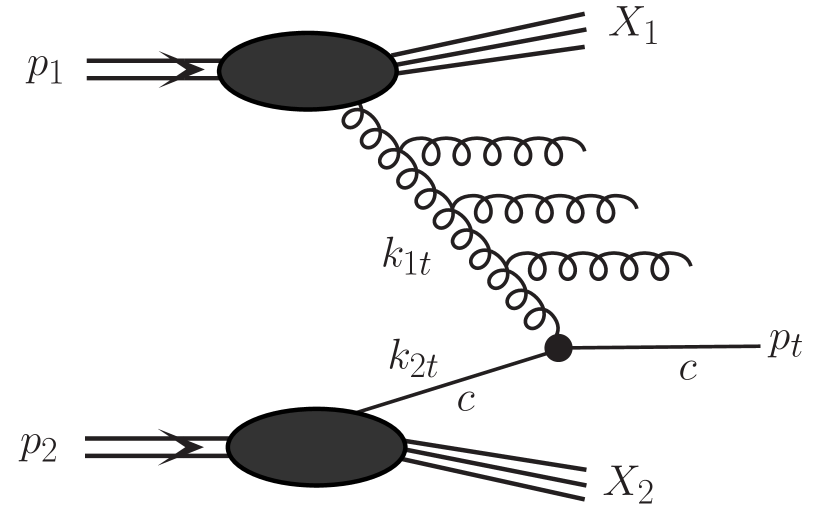
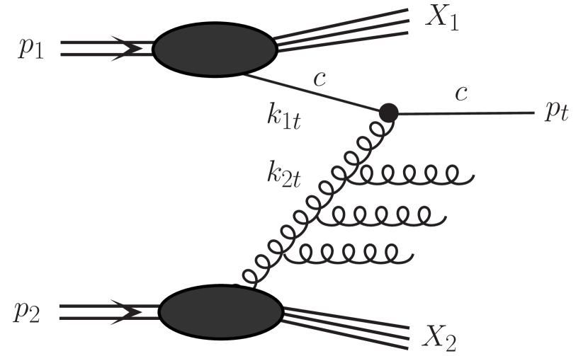
Figure 8: Two leading-order diagrams for charm quark (antiquark) production relevant for $k_{t}$-factorization approach. The extra explicit gluonic emissions suggest the use of unintegrated gluon distributions.

The emitted charm-quark (or antiquark) momentum-space distribution can be written as:

$$\frac{d\sigma(pp\to c\,X)}{dyd^{2}p_{t}} =\frac{16N_{c}}{N_{c}^{2}-1}\cdot\frac{4}{9}\cdot\frac{1}{m_{t}^{2}}\times\;$$

$$\int\alpha_{s}(\Omega^{2})f_{g}(x_{1},k_{1,t}^{2},\mu^{2})f_{c}(x_{2},k_{2,t},\mu^{2})\delta\left(\vec{k}_{1,t}+\vec{k}_{2,t}-\vec{p}_{t}\right)d^{2}k_{1,t}d^{2}k_{2,t}\;.$$

In the formula above $f$’s are unintegrated gluon or charm quark/antiquark distributions. For unintegrated gluon distributions we will take the ones used recently in the literature in the context of $\eta_{c}$ or $\chi_{c}$ production BPSS2019 ; BPSS2020 where the kinematics is similar. For $\Omega^{2}$ we can take $\Omega^{2}=\min(m_{t},k_{1t}^{2},k_{2t}^{2})$ or just $\Omega^{2}=m_{t}^{2}$. The longitudinal momentum fractions are calculated as

$$x_{1} = \frac{m_{t}}{\sqrt{s}}\exp(+y)\;,$$

$$x_{2} = \frac{m_{t}}{\sqrt{s}}\exp(-y)\;.$$ (19)

IV Results

We divide the section with numerical results to four subsections. First three of them are devoted to numerical calculations obtained with the collinear-, hybrid- and the $k_{T}$-factorization approach, respectively. The last subsection contains explicit predictions for impact of intrinsic charm mechanism on forward production of charm in different experiments, including low energy LHC experiments like fixed-target LHCb and SHIP, as well as high energy FCC and LHC experiments, like proposed recently LHC-FASER.

IV.1 The collinear approach

We start presentation of numerical predictions with the results for $pp\to gcX$ reaction driven by the $gc\to gc$ leading-order mechanism calculated in the collinear framework within massive matrix element and kinematics for the energy $\sqrt{s}=7$ TeV. Here we take the gluon and the intrinsic charm distributions as encoded in the CT14nnloIC collinear PDFs. The three different lines in Fig. 9 correspond to a different choice of the $p_{t0}$ parameter used for the regularization of the cross section. We see that the predictions for charm quark transverse momentum (left panel) and rapidity (right panel) distributions are very sensitive to the choice of this parameter, especially, at small charm quark transverse momenta, which also affects the rapidity spectrum. In the numerical studies below $p_{t0}=1.0$ GeV will be taken as a default choice which leads to a central value of the uncertainty related to the choice of the parameter.

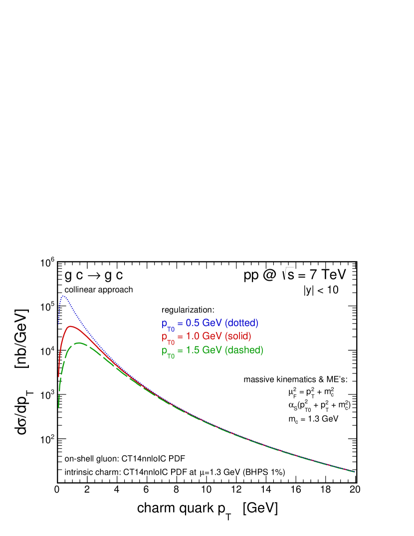
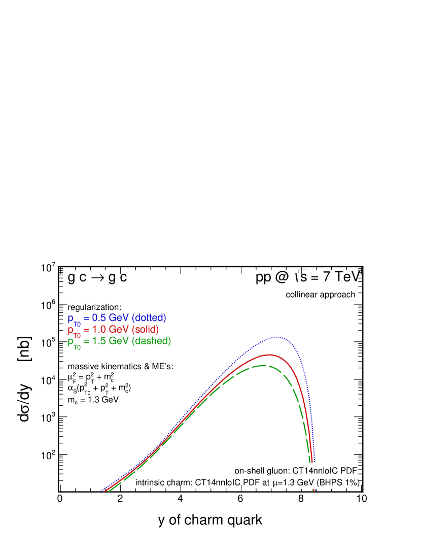
Figure 9: The charm quark transverse momentum (left) and rapidity (right) differential cross sections for $pp$-scattering at $\sqrt{s}=7$ TeV. The results correspond to the $gc\rightarrow gc$ mechanism calculated within the intrinsic charm concept in the collinear-approach with matrix element and kinematics for massive charm quark. Here three different values of the regularization parameter $p_{T0}$ are used. Details are specified in the figure.

In Fig. 10 we present again collinear results for the leading-order $gc\to gc$ mechanism but here we applied four different sets of the intrinsic charm distribution in a proton at initial scale $\mu=1.3$ GeV as incorporated in the CT14nnloIC PDFs. Again, we show the differential cross sections as a function of the charm quark transverse momentum (left panel) and rapidity (right panel). The solid, long-dashed, dotted and dash-dotted lines correspond to the BHPS 1%, BHPS 3.5%, sea-like LS and sea-like HS models, respectively. The sea-like models lead to a larger cross section than in the case of the BHPS model in the midrapidty region. On the other hand, a larger cross section in the forward direction is obtained within the BHPS models. Clearly, large uncertainties due to the intrinsic charm input are found.

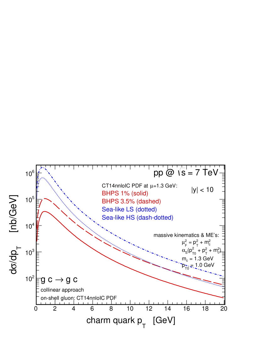
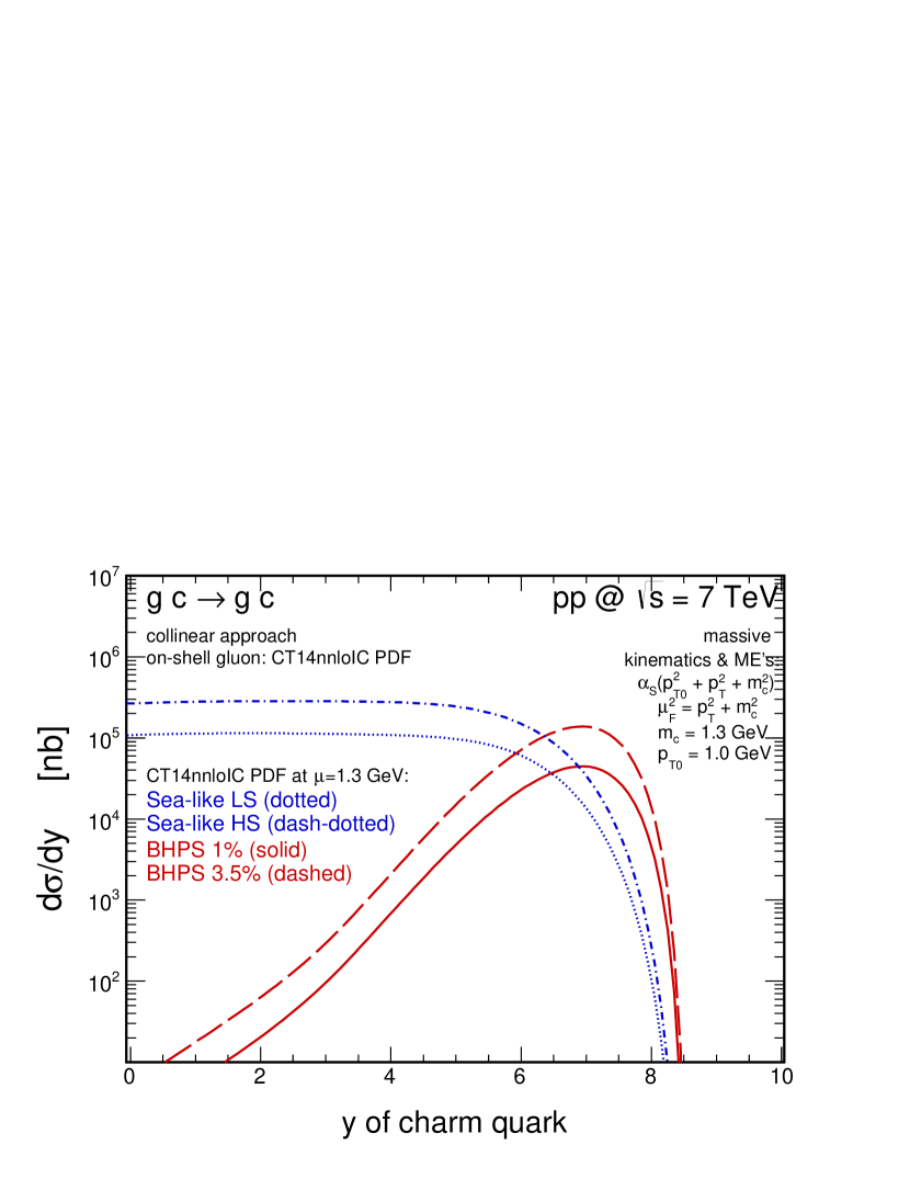
Figure 10: The same as in Fig. 9 but here results obtained with the four different scenarios for intrinsic charm content in a proton are shown. Details are specified in the figure.

The intrinsic charm component in the proton is not the only source of uncertainties related to the collinear PDFs. As it is shown in Fig. 11 the gluon PDF also leads to a significant uncertainties of the predictions. Here we show a comparison of the predictions obtained with the default CT14nnloIC (solid lines), the JR14NLO08VF (dotted lines) and the MMHT2014nlo (dashed lines) PDF sets. The gluon PDFs provided by different groups are probed here at small-$x$ and relatively small scales and lead to a quite different results, especially, at small transverse momenta of charm quark.

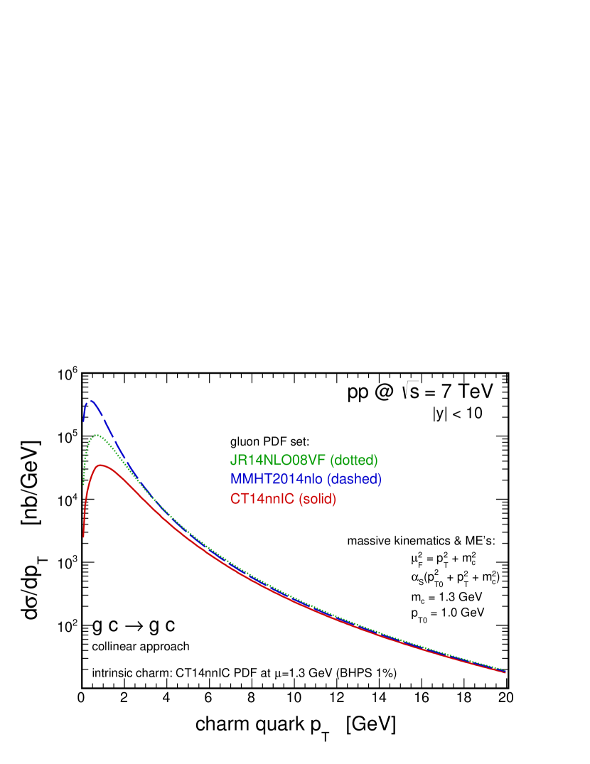
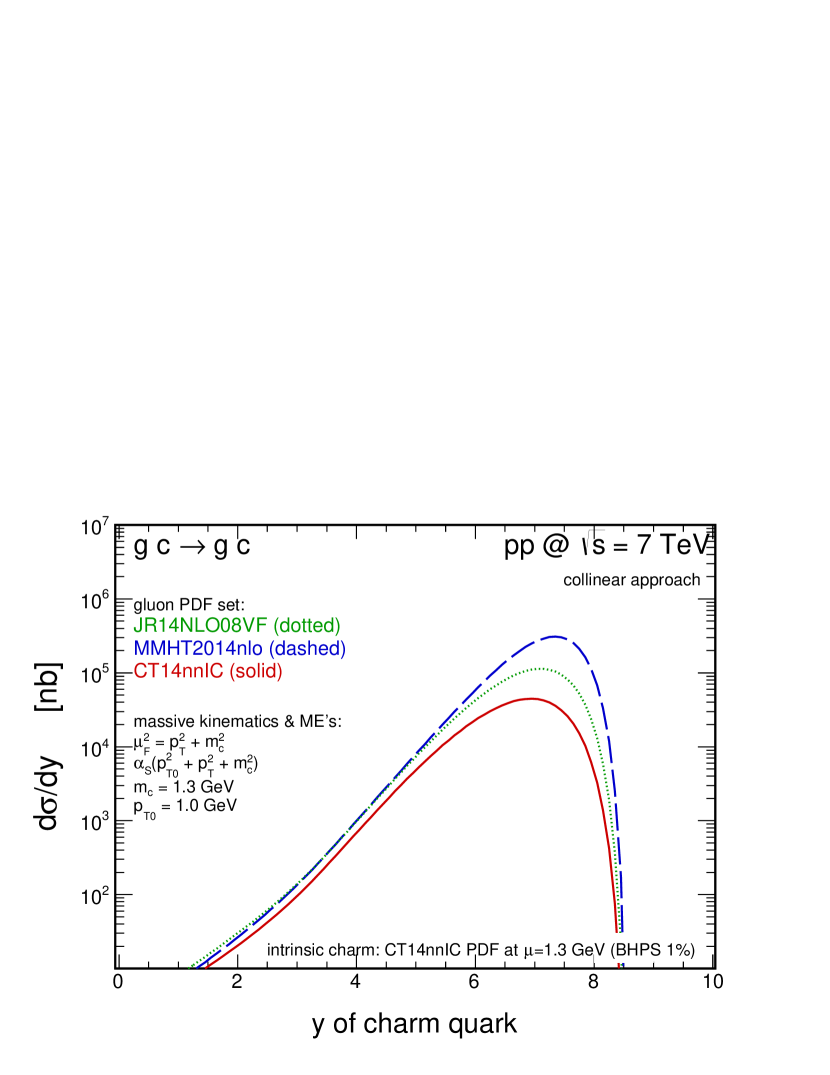
Figure 11: The same as in Fig. 9 but here results obtained with the three different collinear gluon PDFs are shown. Details are specified in the figure.

Now we wish to compare three different schemes for the collinear calculations of the $pp\to gcX$ reaction via the $gc\to gc$ leading-order partonic subprocess. In Fig. 12 we present theoretical distributions obtained within the matrix element with massive quarks (called massive ME for brevity) and kinematics including quark masses (solid lines, our default choice), within the massless matrix element and massless kinematics (dotted histograms), as well as within the massless matrix element and kinematics corrected for the charm quark mass (solid histograms). In each of the cases, we kept the same choice of the renormalization scale $\mu_{R}^{2}=p_{t0}^{2}+p_{t}^{2}+m_{c}^{2}$ and the factorization scale $\mu_{F}^{2}=p_{t}^{2}+m_{c}^{2}$. The charm quark transverse momentum distributions (left panel) are almost identical and some very small (almost invisible) discrepancies appear only at extremely small transverse momenta. The rapidity distributions (right panel) are found to be very sensitive to the charm quark mass effects. Neglecting the charm quark mass in the kinematics leads to a shift of its rapidity distribution to a far forward direction. Correction of the kinematics by inclusion of the outgoing particles mass in the calculation of $x$-values seems to approximately restore the full massive calculations. This step seems to be necessary in the case of massless calculations, otherwise shapes of the predicted rapidity distributions may not be correct.

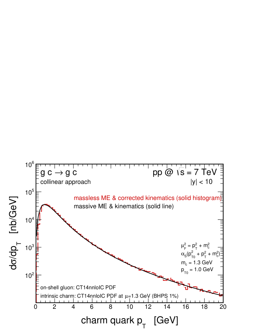
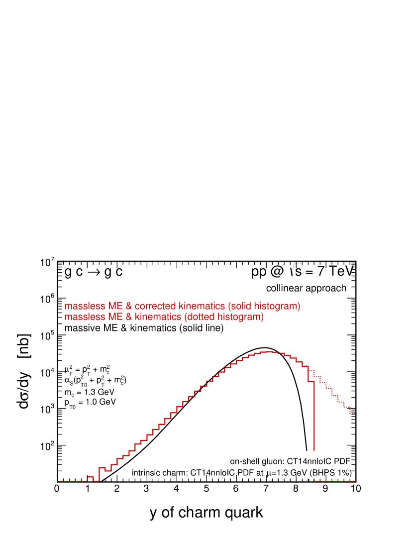
Figure 12: The same as in Fig. 9 but here results of three different schemes of the collinear caclulations are compared. The solid lines correspond to the calculations with massive matrix element and kinematics, the dotted histograms show results for the calculations with massless matrix elements and kinematics, and the solid histograms represent calculations with massless matrix element and kinematics corrected for the charm quark mass.

Having discussed the dominant leading-order mechanism we wish to move beyond and consider importance of higher-order corrections for the charm quark forward production mechanisms with intrinsic charm in the initial state. In Fig. 13 we compare our collinear predictions for the leading-order $2\to 2$ mechanisms, both $gc\to gc$ (dotted histograms) and $qc\to qc$ (short-dashed histograms) shown separately, and for the higher-order $2\to 3$ (long-dashed histograms) and $2\to 4$ (dash-dotted histograms) mechanisms calculated at tree-level. A sum of the four different components denoted as $2\to 2+3+4$ is also shown but it does not follow any merging procedure here. For the higher-order contributions the partonic subprocesses with $gc$ and $qc$ initial states are added together. We report a huge contribution to the cross section coming from the higher-order mechanisms (more than order of magnitude). It clearly shows that the leading-order mechanisms are not enough in order to get reasonable predictions for the impact of intrinsic charm concept on forward charm quark production. Full NLO and even NNLO frameworks are required for precise studies of the subject within the collinear parton model. The situation in the case for other approaches, like the hybrid- and the $k_{T}$-factorization is quite different than in the collinear case what will be discussed in next two subsections.

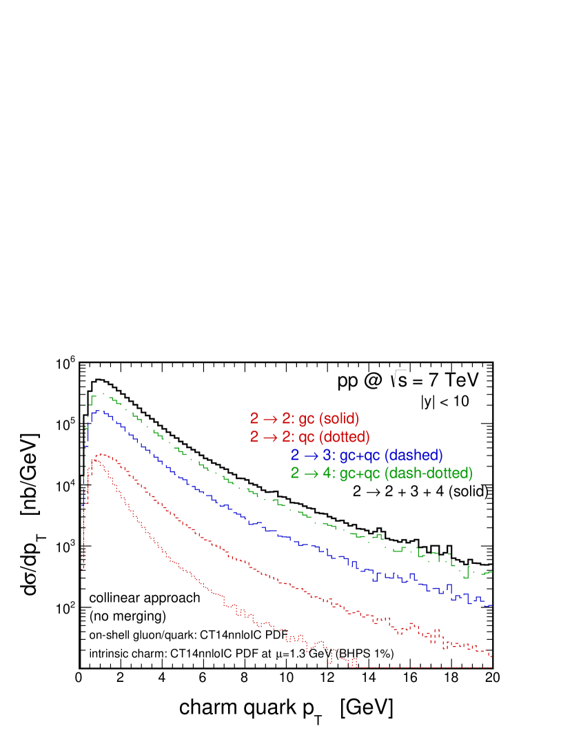
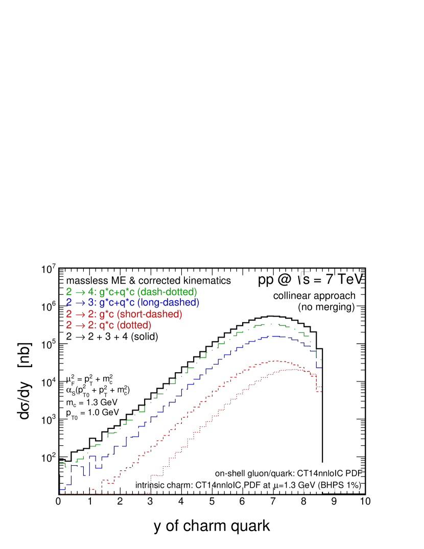
Figure 13: The same as in Fig. 9 but here results of the $2\to 2$ ($gc$ and $qc$ initial states), $2\to 3$ ($gc+qc$ initial states) and $2\to 4$ ($gc+qc$ initial states) mechanisms are shown separately. The calculations are done with massless matrix element and kinematics corrected for the charm quark mass. Details are specified in the figure.

IV.2 The hybrid model

Now we wish to start presentation of our numerical results obtained in the hybrid model. Here the incident small-$x$ parton is assumed to be off-mass shell in contrast to the large-$x$ intrinsic charm which is kept on-shell. In Fig. 14 we show theoretical predictions for charm quark transverse momentum (left panel) and rapidity (right panel) distributions for forward charm production within the leading-order $g^{*}c\to gc$ and the $q^{*}c\to qc$ mechanisms. Here the KMR-CT14lo gluon and light quark/antiquark uPDFs are used. We observe that here much larger cross sections are obtained than in the analogous calculations done in the collinear framework (see two lowest histograms in Fig. 13). Especially, in the hybrid model the gluonic component is much bigger than its collinear counterpart. Significant effects related to the off-shellness of the incident gluons are found. Considering far forward rapidities of the produced charm quark the transverse momenta (virtualities) of the incident small-$x$ gluons start to play a very important role and lead to a sizeable enhancement of the predicted cross section with respect to the leading-order collinear calculations.

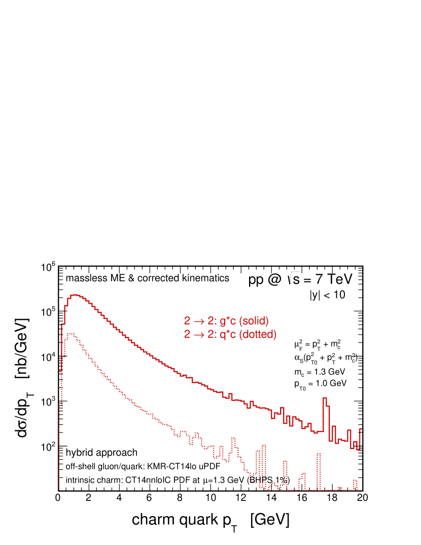
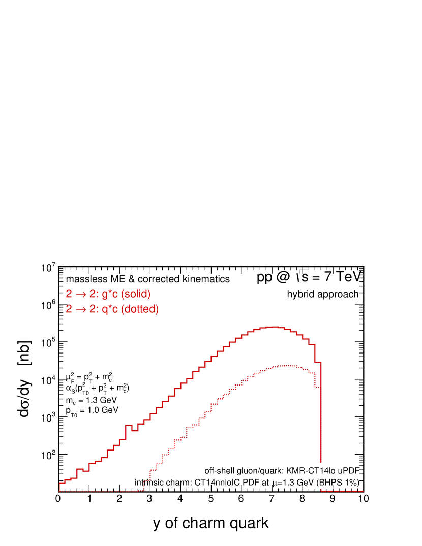
Figure 14: The charm quark transverse momentum (left) and rapidity (right) differential cross sections for $pp$-scattering at $\sqrt{s}=7$ TeV. The results correspond to the $g^{*}c\rightarrow gc$ and $q^{*}c\rightarrow qc$ mechanisms calculated within the intrinsic charm concept in the hybrid model with off-shell initial state gluon and/or off-shell light-quark. Here the KMR-CT14lo unintegrated parton densities were used.

Since in the hybrid model the leading-order quark component $q^{*}c\rightarrow qc$ is found to be negligible one can safely concentrate on the gluonic $g^{*}c\rightarrow gc$ channel only. In Fig. 15 we show the relevant predictions for different unintegrated gluon densities from the literature. We compare results obtained with the KMR-CT14lo (solid histograms), the CCFM JH-2013-set2 (dashed histograms) as well as the KS-linear (dotted histograms) and KS-nonlinear (dash-dotted histograms) gluon uPDFs. Different models lead to quite different results, however, they seem to be consistent with each other up to a factor of 5. Main differences appear at larger quark transverse momenta. At small transverse momenta predictions within the KMR-CT14lo, the JH-2013-set2 and the KS-linear uPDFs coincide. It translates also into the rapidity spectrum. Only the KS-nonlinear uPDF leads to a somewhat different behaviour of the cross section at small $p_{T}$’s. We observe that both the transverse momentum and rapidity distributions of charm quark are sensitive to the non-linear evolution effects that lead here to a sizeable damping of the predicted cross section. Thus, the forward production of charm within intrinsic charm concept might be a very good testing ground for studies of the non-linear term in the evolution of unintegrated gluon densities and may shed new light on phenomenon of parton saturation.

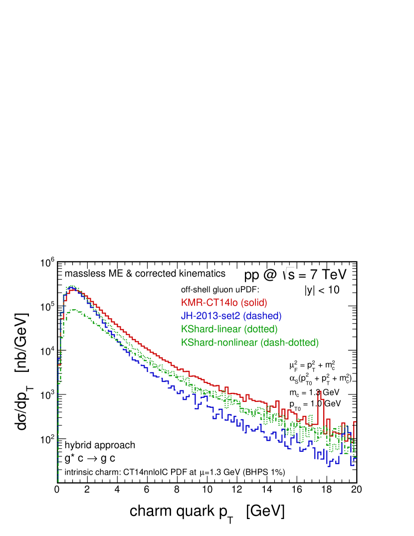
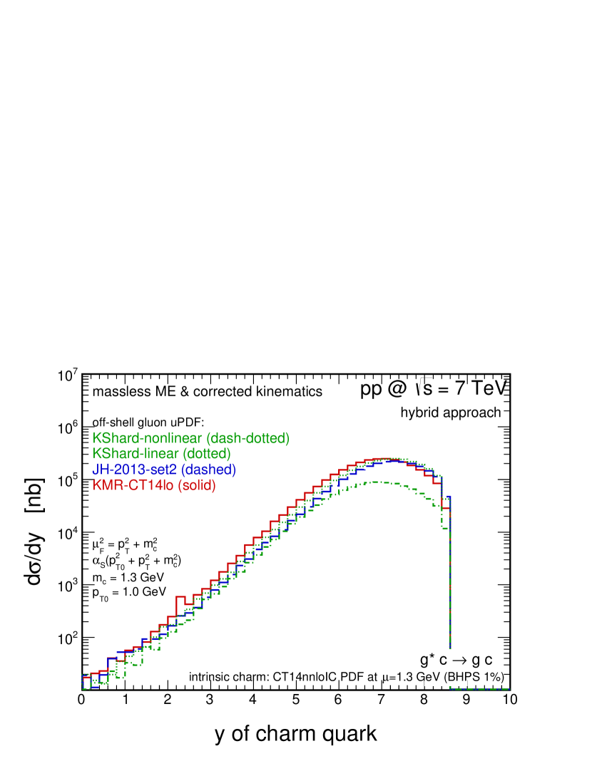
Figure 15: The same as in Fig. 14 but here results for four different unintegrated gluon densities in a proton are shown. Here only the $g^{*}c\rightarrow gc$ mechanism is taken into account.

Above, we have used those gluon uPDF models that are assumed to allow for an effective resummation of extra real emissions (real higher-order terms). Therefore, their can be successfully used in phenomenological studies based even on leading-order matrix elements (see a discussion in Refs. Maciula:2019izq ; Maciula:2020cfy ). Here we wish to present results obtained within the scheme of the calculations where the higher-order corrections are not resummed in the uPDF but are taken into account via the hard-matrix elements. This procedure can be tested with the help of the DGLAP-based Parton-Branching uPDFs as was proposed in Ref. Maciula:2019izq and further applied in Refs. Lipatov:2019izq ; Maciula:2020cfy . In Fig. 16 we show predictions of the hybrid model for the $2\to 2$, $2\to 3$ and $2\to 4$ mechanisms, as well as for their sum $2\to 2+3+4$ obtained using a dedicated merging procedure. The results are calculated with the PB-NLO-set1 quark and gluon uPDFs. For the leading-order $2\to 2$ mechanisms we show $g^{*}c$ and $q^{*}c$ channels separately while for the higher-order components we plot sum of all possible gluonic and quark channels. As in the collinear case, the higher-order mechanisms are found to be very important also here.

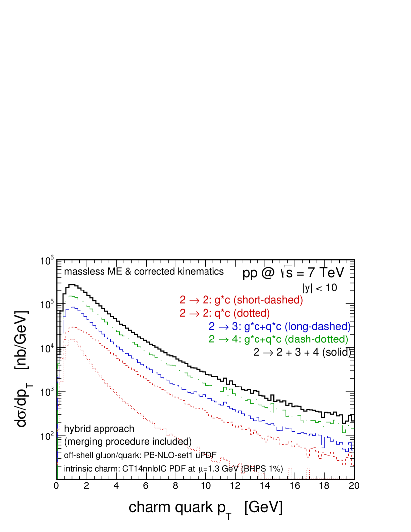
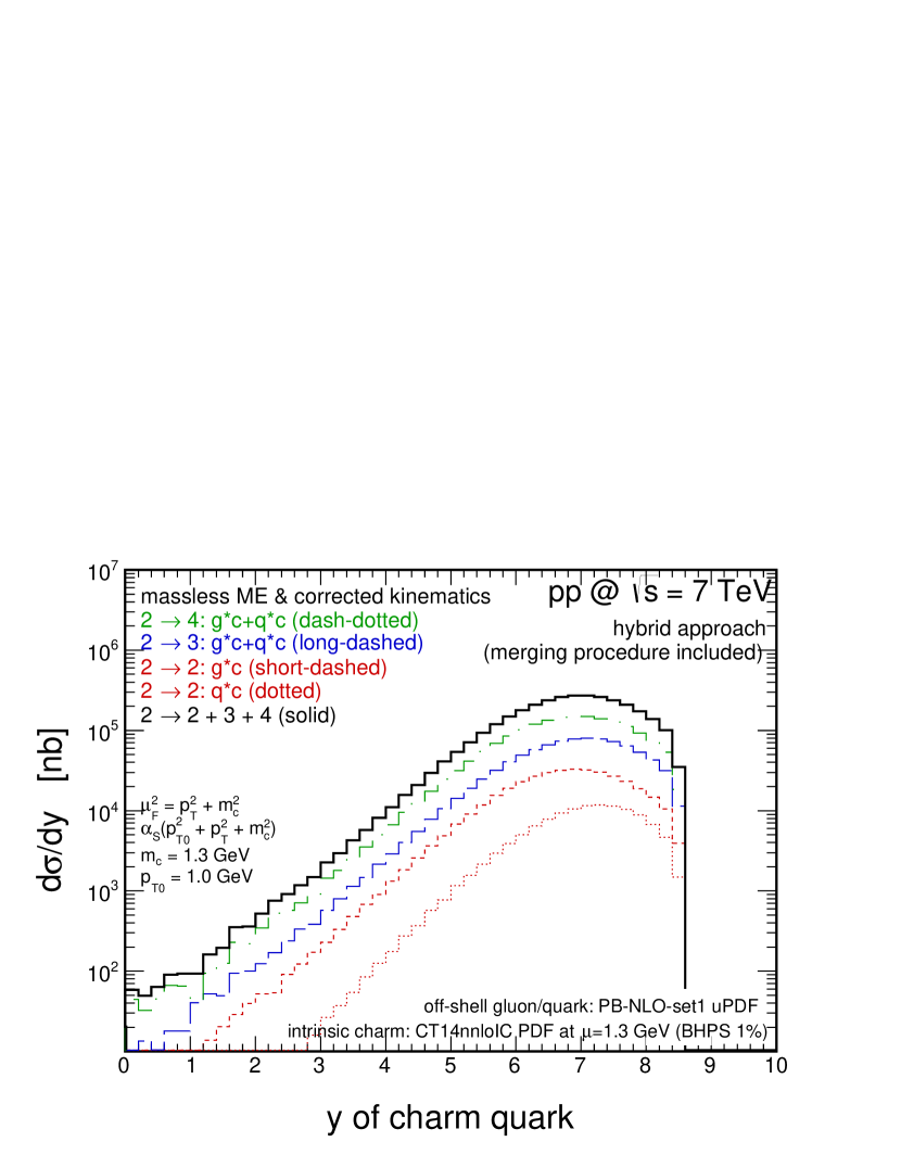
Figure 16: The same as in Fig. 14 but here results for PB-NLO-set1 unintegrated parton densities obtained within the $2\to 2+3+4$ scheme of the calculation. Here, the $2\to 2$, $2\to 3$, and $2\to 4$ components as well as their sum $2\to 2+3+4$ obtained including merging procedure are shown separately.

For a better transparency in Fig. 17 we compare the hybrid model results obtained with the KMR-CT14lo (solid histograms) with the PB-NLO-set1 (dashed histograms) uPDFs, that correspond to the two different hybrid calculation schemes, together with the results obtained in the collinear approach (dotted histograms). Both types of the hybrid model calculations seem to lead to a very similar predictions. It seems to justify the proposed $2\to 2+3+4$ hybrid calculation scheme with the PB uPDFs and with the applied merging in a qualitative way. On the other hand, the collinear $2\to 2+3+4$ results seem to be larger by a factor of 2 than their hybrid model counterpart. However, this might be related to a lack of a relevant merging procedure in the collinear case.

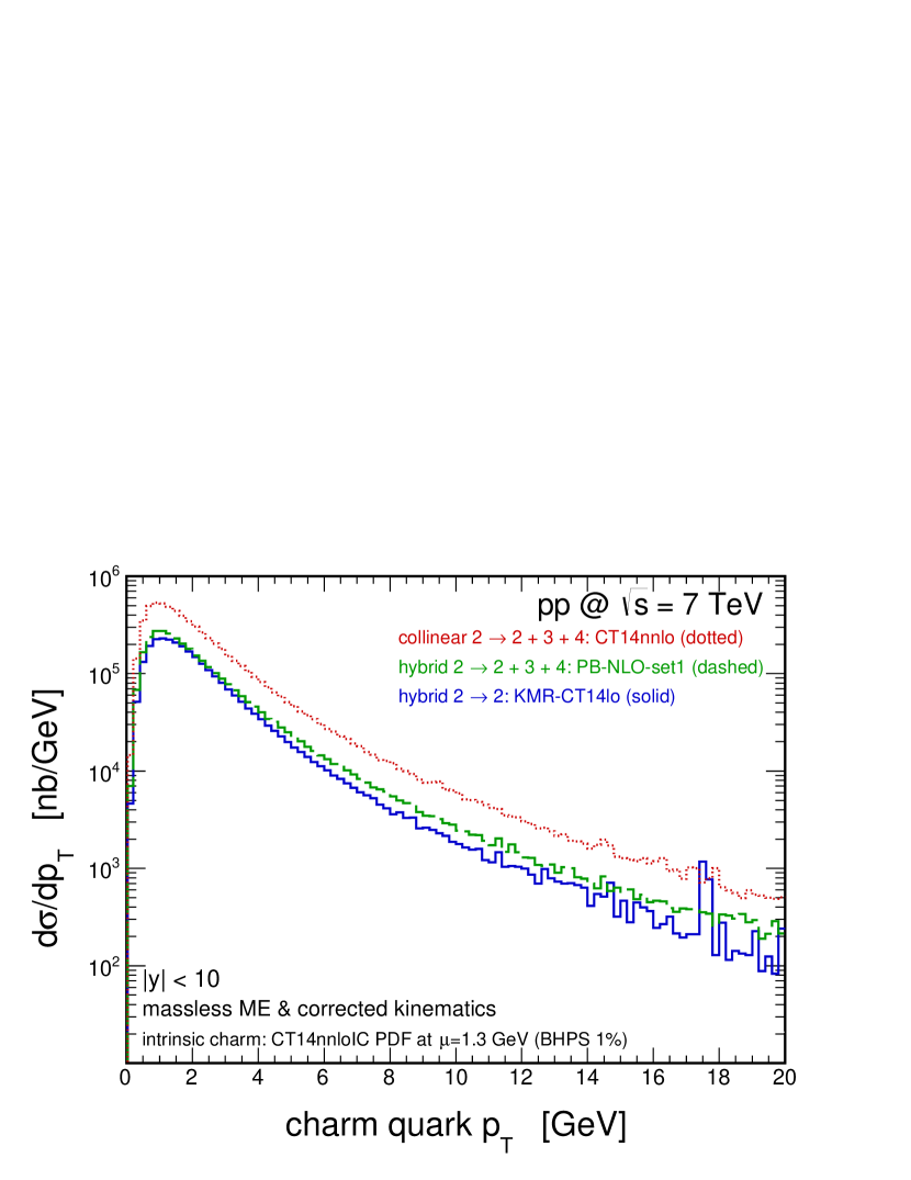
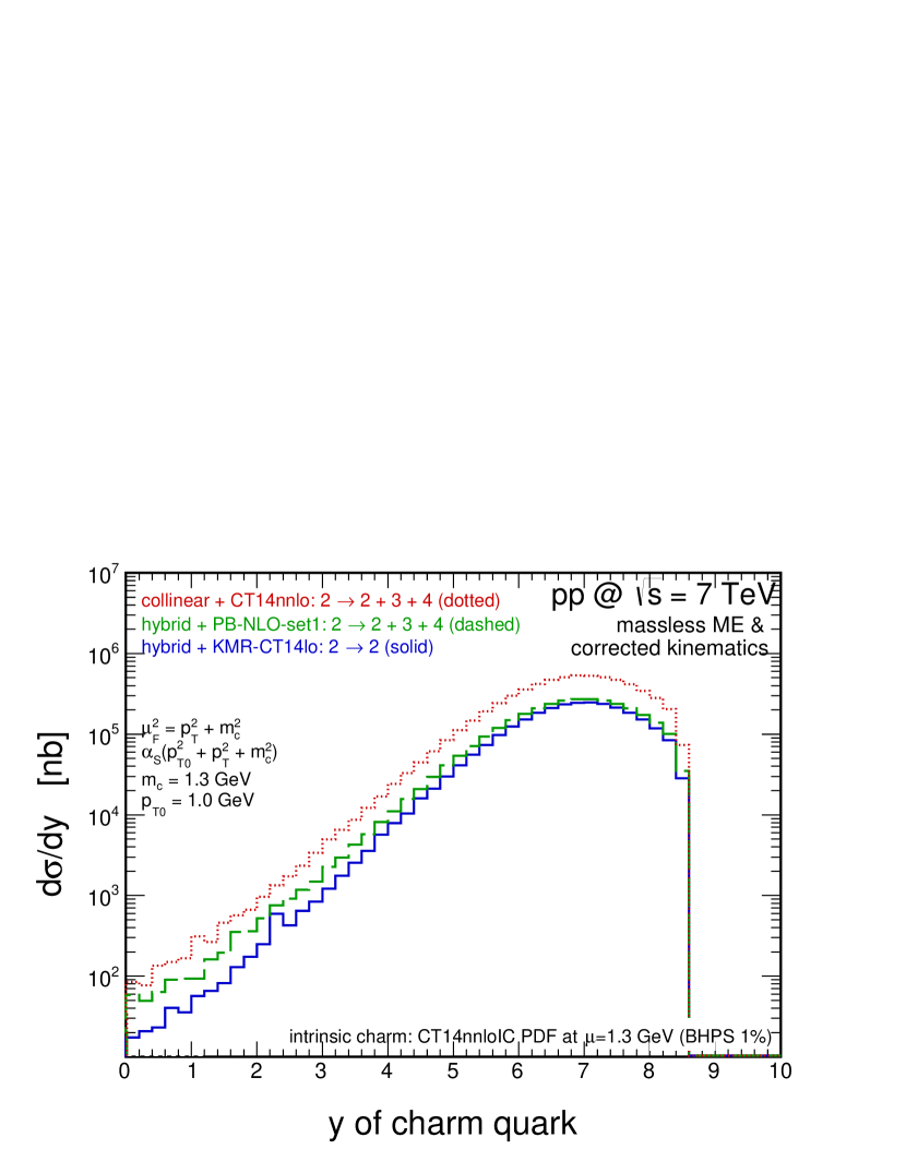
Figure 17: The same as in Fig. 14 but here we compare results for the CT14nnlo collinear PDFs with $2\to 2+3+4$ collinear model calculations, for the KMR-CT14lo uPDFs with the $2\to 2$ hybrid model calculations and for the PB-NLO-set1 uPDFs with $2\to 2+3+4$ hybrid model calculations including merging.

IV.3 The $\bm{k_{T}}$-factorization approach

Now we wish to present results obtained within the $k_{T}$-factorization approach. So here we take into account also effects related to off-shellness of $c$ quark of the intrinsic charm in the proton. The transverse momentum dependent intrinsic charm uPDF is obtained by Gaussian smearing of the collinear PDF. Rather small smearing parameter is used that do not allow for a large transverse momenta of the intrinsic charm. It seems to be appropriate for the case of the forward production of charm. For the unintegrated gluon density the KMR-CT14lo model is used.

In Fig. 18 we show predictions for the $g^{*}c^{*}\to gc$ mechanism with both initial state partons being off-shell. Here three different values of the smearing parameter in the calculation of the intrinsic charm uPDF are used: $\sigma_{0}=0.5$ GeV (solid histograms), $3.5$ GeV (dotted histograms) and $7.0$ GeV (dashed histograms). The larger $\sigma_{0}$ is taken the smaller cross section at small outgoing charm quark transverse momenta is obtained (left panel). The same is true for the rapidity spectrum in the forward region (right panel).

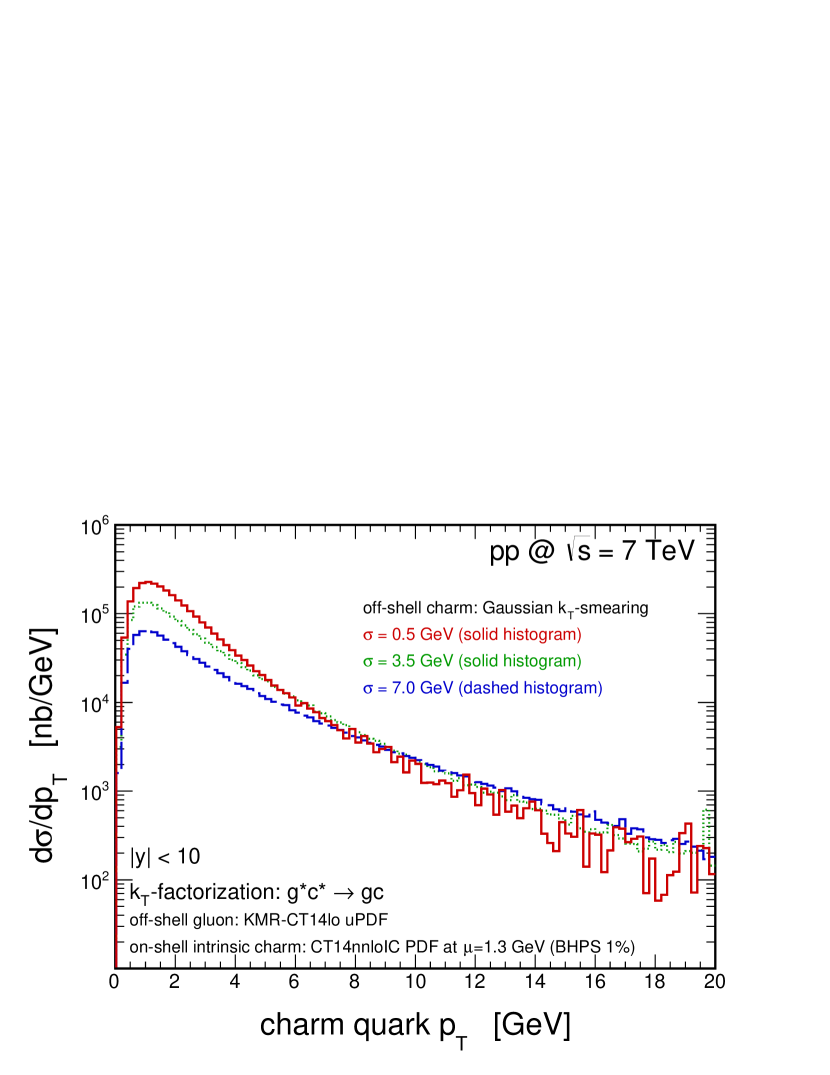
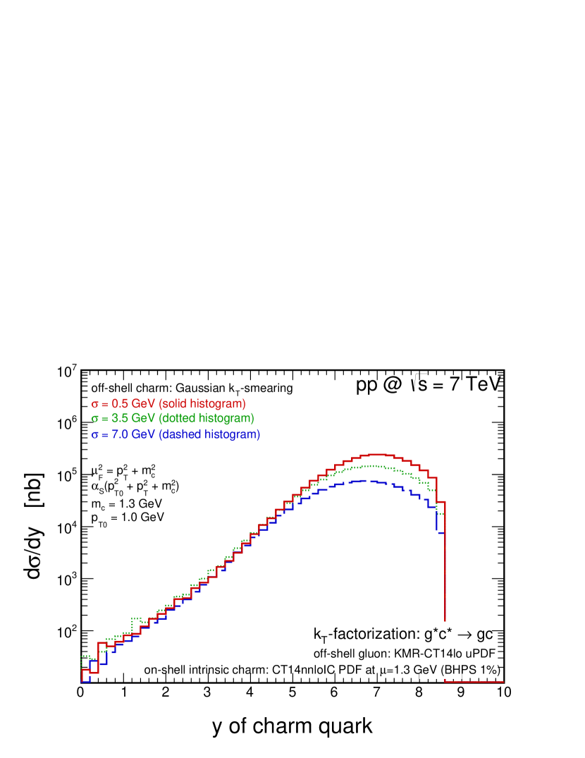
Figure 18: The charm quark transverse momentum (left) and rapidity (right) differential cross sections for $pp$-scattering at $\sqrt{s}=7$ TeV. The results correspond to the $g^{*}c^{*}\rightarrow gc$ mechanism calculated within the intrinsic charm concept in the $k_{T}$-factorization approach with both off-shell initial state partons. Here the KMR-CT14lo unintegrated gluon density and Gaussian $k_{t}$-distribution for off-shell charm quark were used. We show results for different values of the smearing parameter $\sigma$.

In Fig. 19 we illustrate mutual relations between the results obtained with the hybrid and the $k_{T}$-factorization frameworks. When the smearing parameter in the calculation of the intrinsic charm uPDF is small, e.g. $\sigma_{0}=0.5$ GeV, the hybrid model $g^{*}c\to gc$ results coincide with the $g^{*}c^{*}\to gc$ results obtained within the full $k_{T}$-factorization approach.

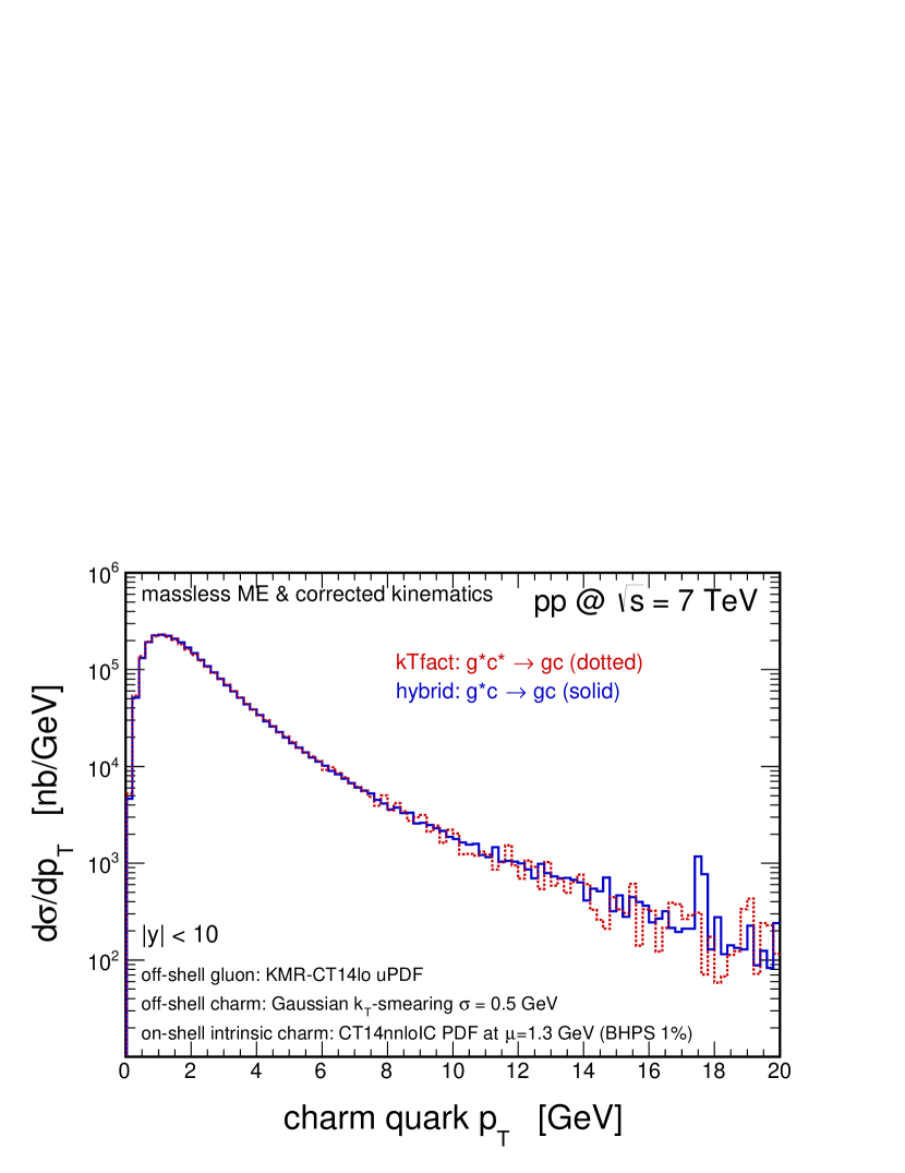
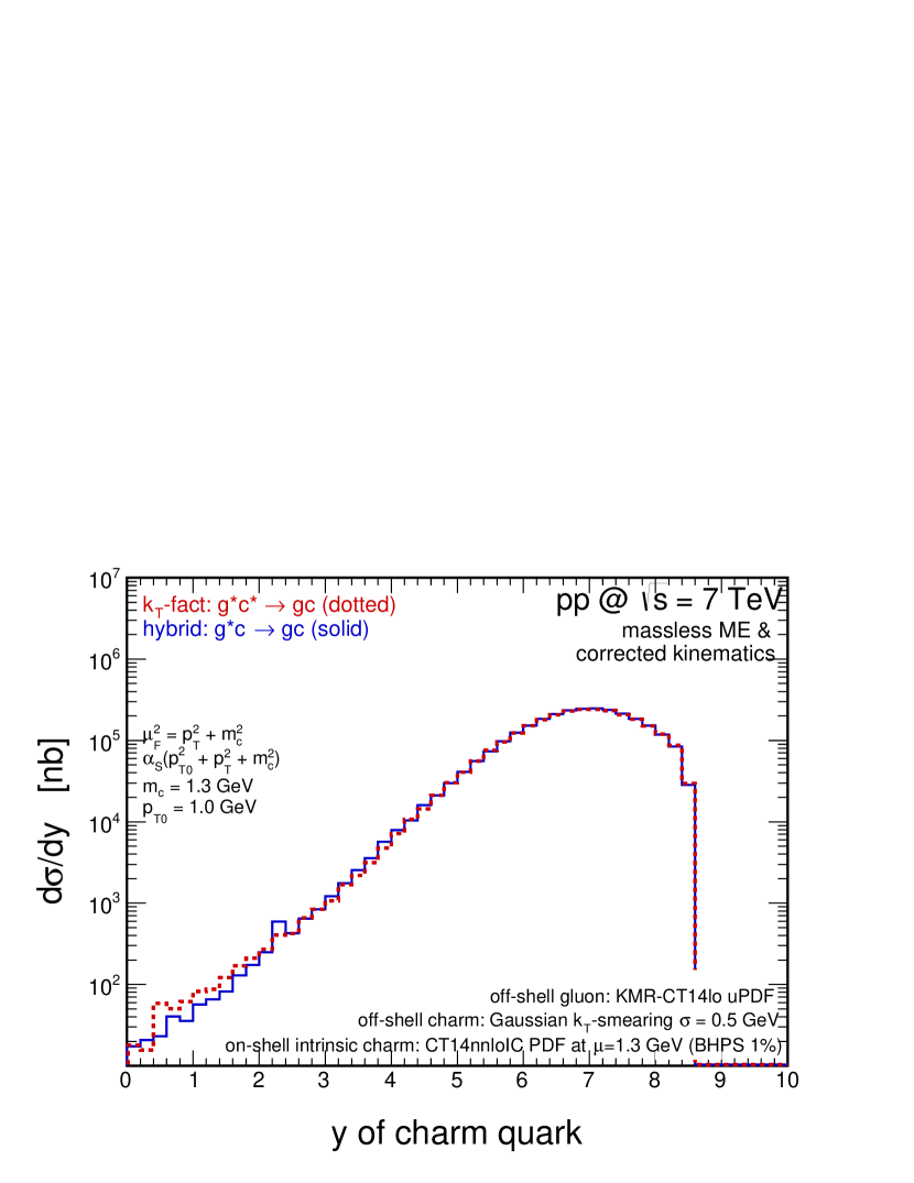
Figure 19: The same as in Fig. 18 but here we compare results for the hybrid $g^{*}c\to gc$ and the $k_{T}$-factorization $g^{*}c^{*}\to gc$ calculations obtained with the KMR-CT14lo unintegrated gluon densities. The off-shell charm quark Gaussian $k_{t}$-distribution is obtained with the the smearing parameter $\sigma_{0}=0.5$ GeV.

Finally, we wish to present results of the $k_{T}$-factorization approach for the $g^{*}c^{*}\to c$ mechanism. In Fig. 20 we compare the corresponding predictions obtained with the four different gluon uPDFs: the KMR-CT14lo (solid lines), the JH-2013-set2 (dotted lines), the KS-linear (dash-dotted lines) and the KS-nonlinear (dashed lines). Different models lead to quite different results. The discrepancies between the uPDF models obtained here seem to be larger than in the corresponding case of the $g^{*}c\to gc$ calculations within the hybrid model.

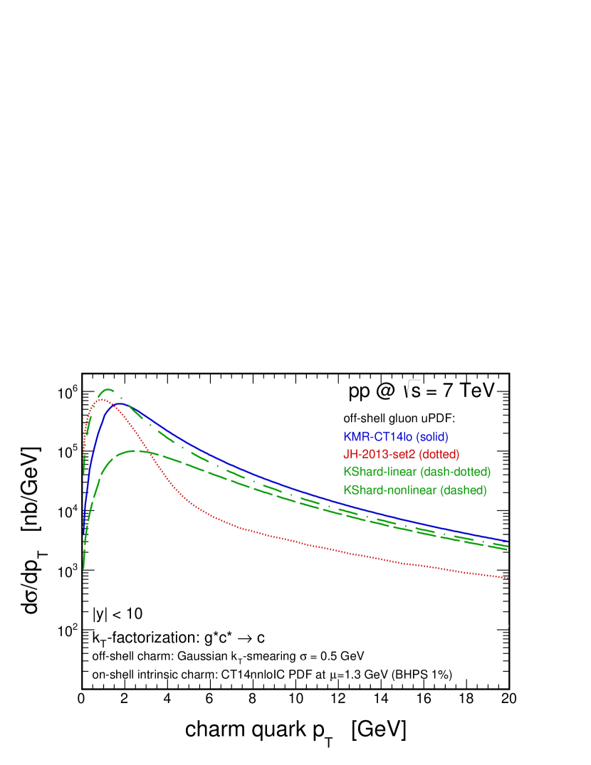
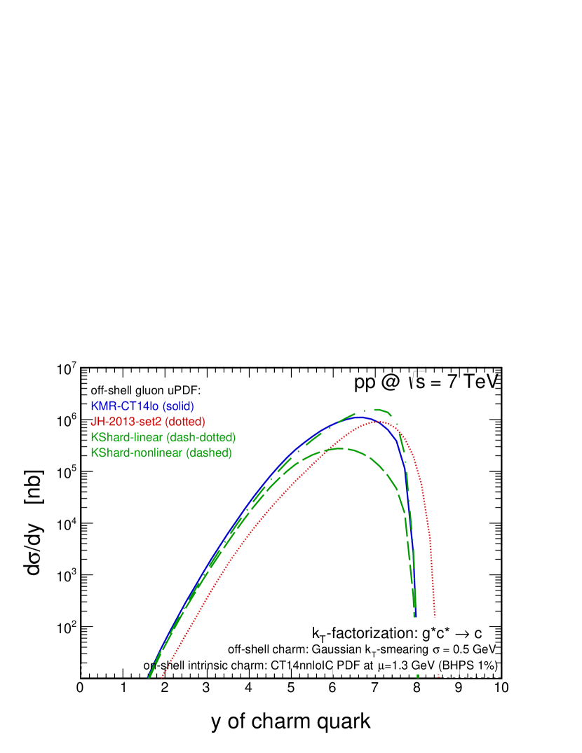
Figure 20: The charm quark transverse momentum (left) and rapidity (right) differential cross sections for $pp$-scattering at $\sqrt{s}=7$ TeV. The results correspond to the $g^{*}c^{*}\rightarrow c$ mechanism calculated within the intrinsic charm concept in the $k_{T}$-factorization approach with both off-shell initial state partons. Here the Gaussian $k_{t}$-distribution for off-shell charm quark were used. We show results for different gluon uPDFs.

IV.4 Predictions for future experiments

Before we go to predictions for different future and present experiments we wish to summarize the conclusions drawn in the previous subsection by a direct comparison of the results corresponding to the approaches discussed above.

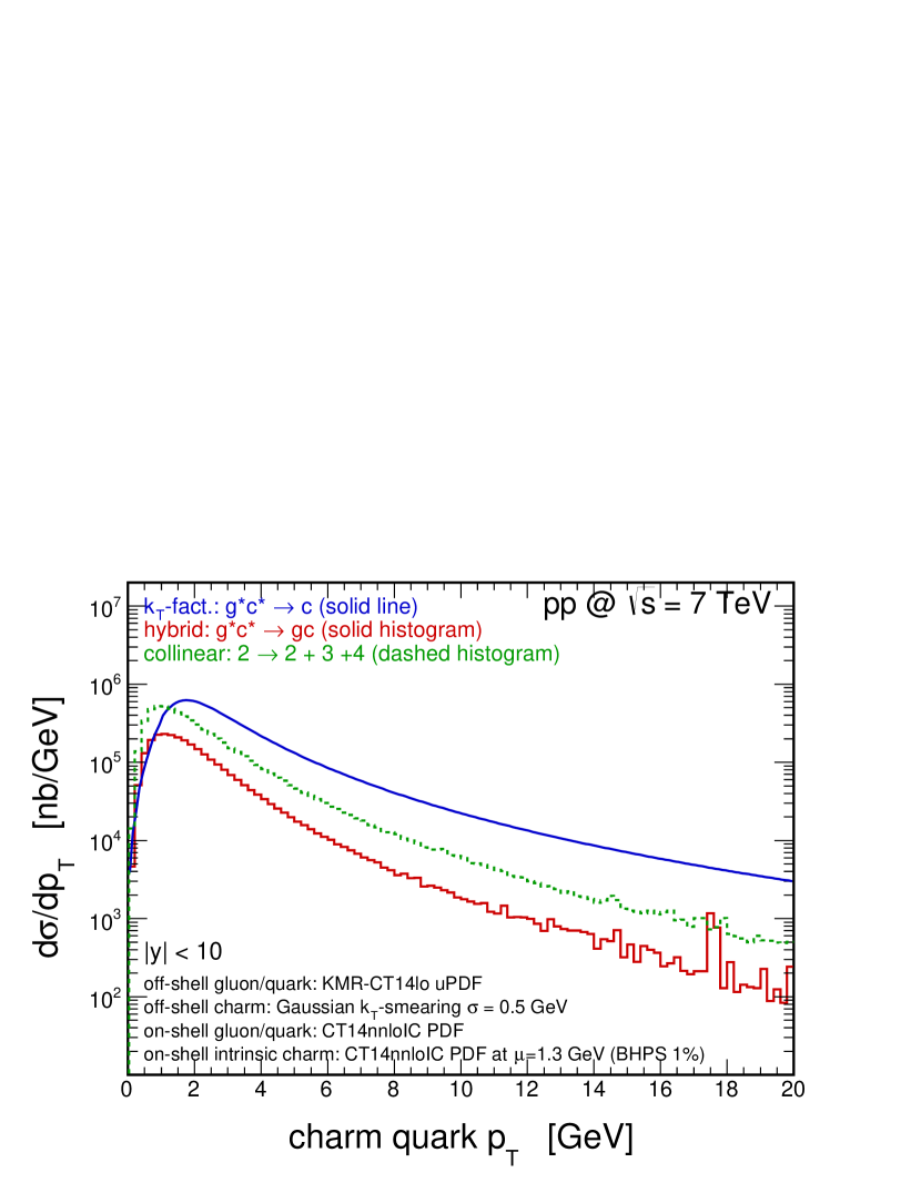
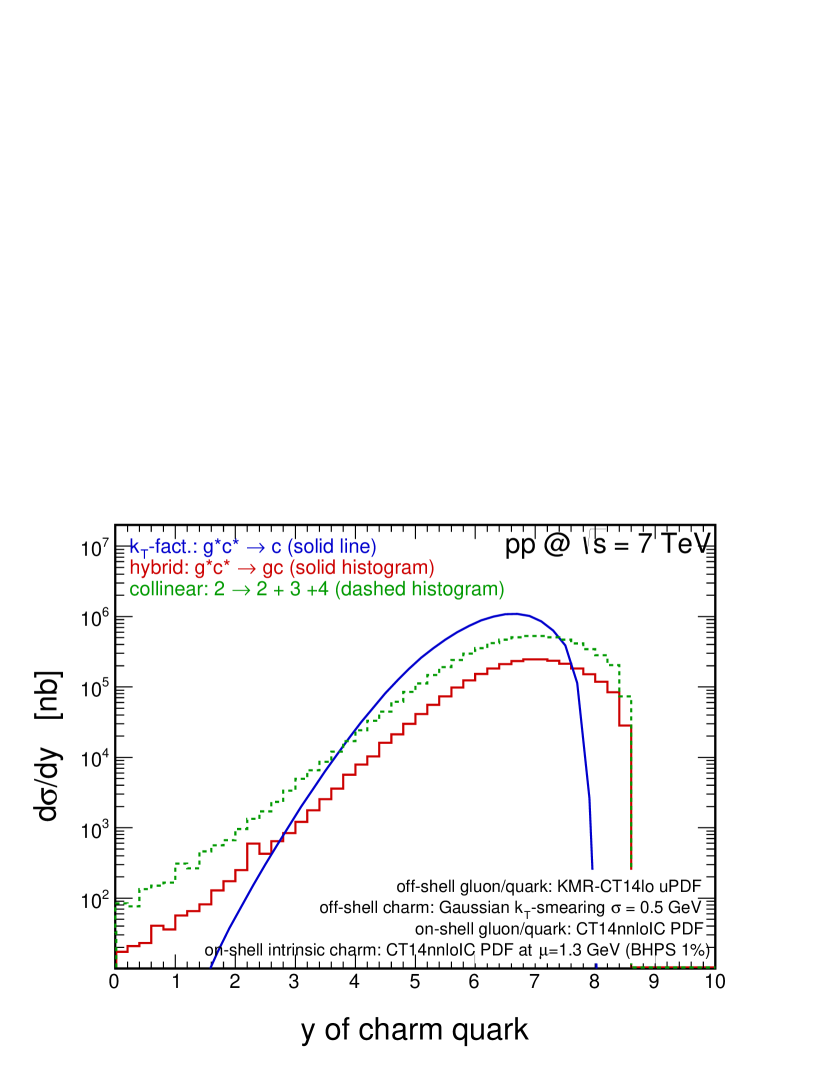
Figure 21: The charm quark transverse momentum (left) and rapidity (right) differential cross sections for $pp$-scattering at $\sqrt{s}=7$ TeV. Here we compare predictions of the three different approaches used in the previous subsections: the $2\to 2+3+4$ collinear, the hybrid $g^{*}c\to gc$ and the $k_{T}$-factorization $g^{*}c^{*}\to c$ calculations.

In Fig. 21 we compare predictions of the three different approaches used in the previous subsections: the $2\to 2+3+4$ collinear (dashed histograms), the hybrid $g^{*}c\to gc$ (solid histograms) and the $k_{T}$-factorization $g^{*}c^{*}\to c$ (solid lines) calculations. Different models lead to a very different results with more than one order of magnitude difference between the lowest and the highest predicted cross section. Huge cross section for $gc\to c$ or $cg\to c$ may be partly due to ignoring other emissions than $c$ or $\bar{c}$ in the evolution of $x_{1}$ and $x_{2}$. These large uncertainties of the predictions can be reduced only by a forward experiments at forward directions. Forward charm production data sets that will be dominated by the contribution from intrinsic charm are necessary to draw definite conclusions about the level of applicability of the different theoretical approaches.

Therefore, now we wish to present results of the study of the impact of the intrinsic charm component on the forward charm particle production in already existing or future experiments at different energies. We start with predictions for the high energy experiments at the LHC and the FCC, at $\sqrt{s}=13$ and $50$ TeV, respectively (top and bottom panels in Fig. 22). In the LHC case the considered kinematics correspond to the planned FASER experiment. Here we compare predictions of the $k_{T}$-factorization approach for the $g^{*}g^{*}\to c\bar{c}$ mechanism which is known to give a very good description of the LHC open charm data Maciula:2019izq , and predictions of the $g^{*}c\to gc$ mechanism (dashed) within the hybrid model. In both cases the charm production cross section starts to be dominated by the intrinsic charm component at very forward rapidities, i.e. $y\geq 7$. In this far-forward region, the transverse momentum distribution of charm quark is also dominated by the contributions of the intrinsic charm. The predicted enhancement of the charm cross section could certainly be examined by the FASER experiment dedicated to a measurement of forward neutrinos originating from semileptonic decays of $D$ mesons. The actual predictions for neutrinos will be presented elsewhere.

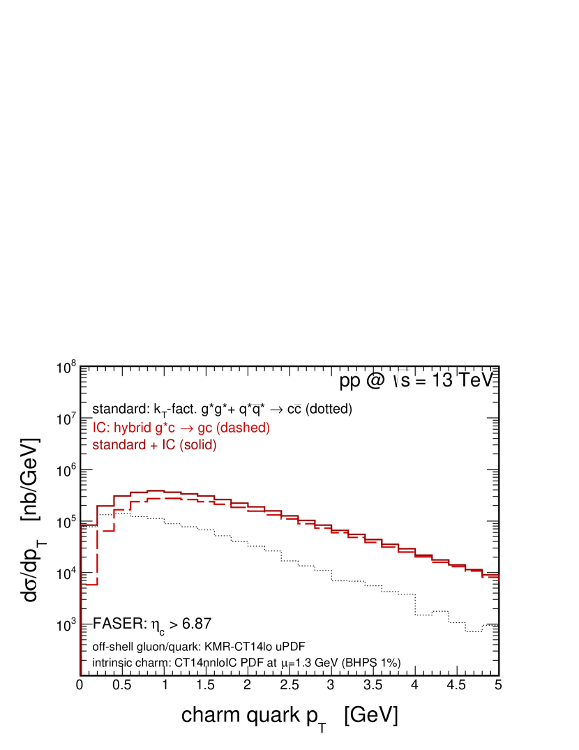
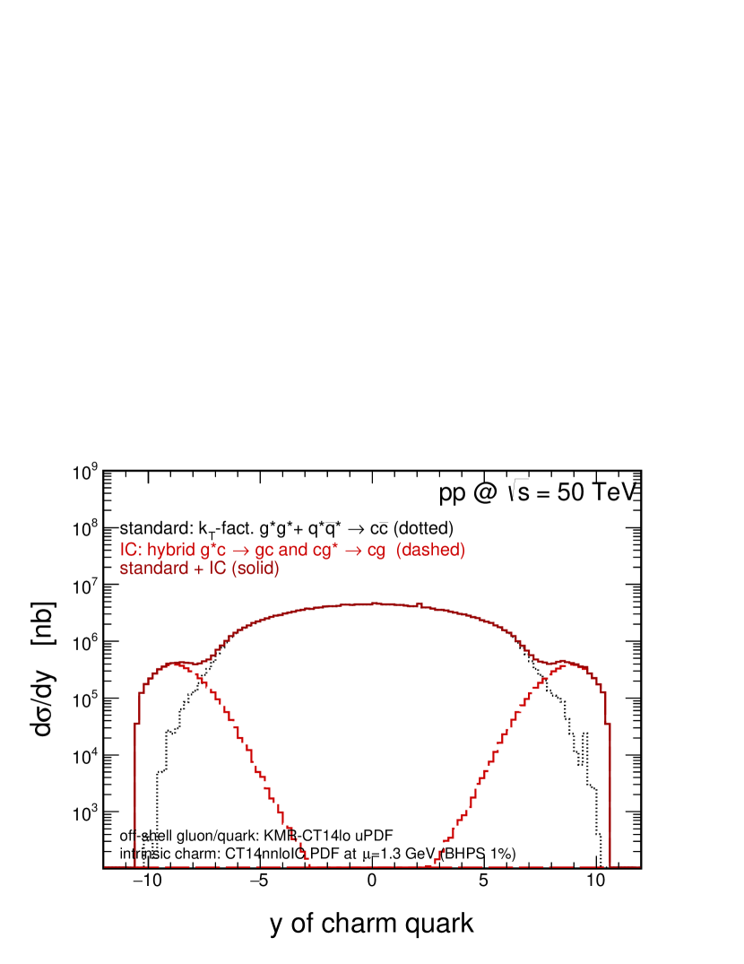
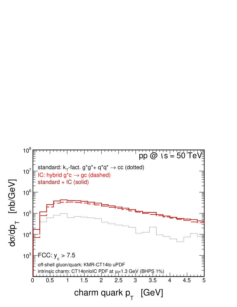
Figure 22: Predictions of the impact of the intrinsic charm component in charm quark production in different experiments. Here we explore kinematics relevant for the FASER experiment at the LHC and an exemplary experiment at the FCC.

In addition, we also analysed a possibility of experimental study of the intrinsic charm concept at lower energies. In Fig. 23 we show predictions for the fixed-target LHC and the SHIP experiment, at $\sqrt{s}=86.6$ and $27.4$ GeV, respectively (top and bottom panels). We observe that also at relatively small energies the intrinsic charm contributions could be identified experimentally. It seems that the already existing data set on open charm meson production in the fixed-target LHC mode Aaij:2018ogq needs to have the intrinsic charm component included in the theoretical description. Similarly, our results suggests that the predictions of the tau-neutrino flux that could be measured in the SHIP experiment should include effects related to a possible intrinsic charm content of the proton.

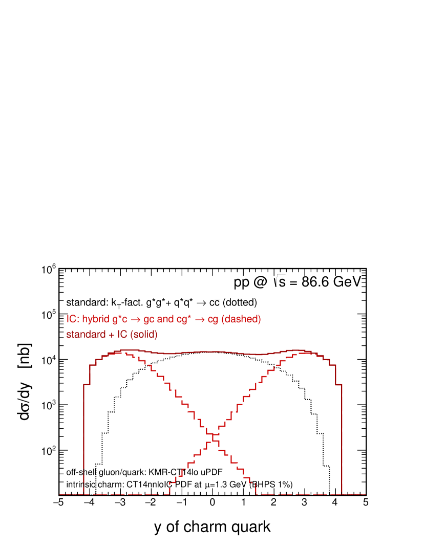
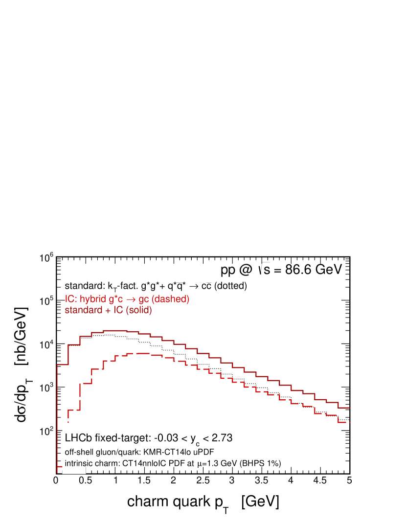
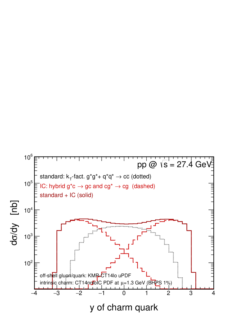
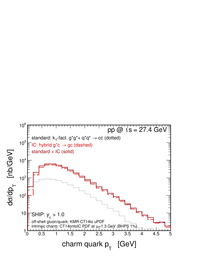
Figure 23: Predictions of the impact of the intrinsic charm component in charm production in different experiments. Here we explore kinematics of the fixed-target mode LHCb and the kinematics relevant for the SHIP experiment.

V Conclusions

In this paper we have discussed the effect of intrinsic charm in the proton on forward production of $c$ quark or $\bar{c}$ antiquark at different energies. Three different approaches: collinear, hybrid and $k_{T}$-factorization have been used with modern collinear and unintegrated parton distribution functions.

The production mechanism of $c$-quarks and $\bar{c}$-antiquarks originating from intrinsic charm in the nucleon is concentrated in forward/backward directions, but details depend on collision energy. The absolute normalization strongly depends on the approach used. The leading-order (LO) collinear framework leads to the smallest cross section. The cross section becomes much bigger in the $k_{T}$-factorization or in the hybrid model which effectively include higher-order corrections. The next-to-leading (NLO) and even next-to-next-to-leading (NNLO) tree-level corrections are found to be very important here. Therefore, the $k_{T}$-factorization or the hybrid model will give stringent limits on the intrinsic charm which cannot be constrained at present from first principles.

We have shown that in the collinear approach the LO calculations of the intrinsic charm component are insufficient. We have included the NLO and NNLO components at tree-level which were found to significantly contribute to the cross section.

Working in the hybrid model or in the $k_{T}$-factorization approach we have shown that the effects related to the off-shellness of the incident partons (especially gluons) are large. In both cases higher-order corrections are effectively included already within the basic $gc\to gc$ mechanism. We have used different models for gluon unintegrated parton distribution functions (uPDFs) from the literature. We obtained different results for different gluon uPDFs. The forward charm production was recognized as a useful testing ground for the small-$x$ behaviour of the gluon uPDFs. We have shown in addition that the final results are also sensitive to the concept of gluon saturation in a proton. Unintegrated gluon densities derived from linear and non-linear evolution equations lead to a quite different results. We have performed also leading-order calculations within $k_{T}$-factorization approach where the basic process is either $g+c\to c$ or $c+g\to c$ as done for forward production of charm quarks.

We have shown that the intrinsic charm component dominates over the standard pQCD (extrinsic) mechanism of $c\bar{c}$-pair production at forward (or far-forward) rapidities starting from low energy fixed-target experiment at $\sqrt{s}=27.4$ and $86.6$ GeV, through the LHC Run II nominal energy $\sqrt{s}=13$ TeV, and up to the energies relevant for the IceCube experiment ($\sqrt{s}=50$ TeV). The LHC experiments at low energies (fixed-target experiments) can provide valuable information already now. Future LHC experiments on $\nu_{\tau}$ neutrino production such as SHIP sand FASER are an interesting alternative in next few years.

In the present study we intentionally limited to the production of charm quarks/antiquarks. The production of charmed mesons or baryons is currently uder discussion and a new fragmentation scheme was proposed szczurek2020 very recently. We leave the predictions for production of charmed hadrons and their semileptonic decays for a separate study. However, the consequences for high-energy neutrino production have been discussed shortly in the context of the IceCube experiment and experiments proposed at the LHC (SHIP and FASER).

References

- (1) S.J. Brodsky, P. Hoyer, C. Peterson and N. Sakai, Phys. Lett. B93, 451 (1980).
- (2) V.D. Barger, F. Halzen and W.Y. Keung, Phys. Rev. D25, 112 (1982).
- (3) R. Vogt and S.J. Brodsky, Nucl. Phys. B438, 261 (1995), 478, 311 (1996).
- (4) F.S. Navarra, M. Nielsen, C.A.A. Nunes and M. Teixeira, Phys. Rev. D54, 842 (1996).
- (5) W. Melnitchouk and A.W. Thomas, Phys. Lett. B414, 134 (1997).
- (6) F.M. Steffens, W. Melnitchouk and A.W. Thomas, Eur. Phys. J. C11, 673 (1999).
- (7) F. Carvalho, F.O. Duraes, F.S. Navarra and M. Nielsen, Phys. Rev. Lett. 86 (2001) 5434.
- (8) T.J. Hobbs, J.T. Londergan and W. Melnitchouk, Phys. Rev. D89, 074008 (2014).
- (9) R.S. Sufian, T. Liu, A. Alexandru, S.J. Brodsky, G.F. de Teramond, H. G. Dosch, T. Draper, K.-F. Liu and Y.-B. Yang. arXiv:2003.01078 [hep-lat].
- (10) P.H. Beauchemin, V.A. Bednyakov, G.I. Lykasov, Y.Y. Stepanenko, Phys. Rev. D92, 0341014 (2015).
- (11) S. Rostami, A. Khorramian, A. Aleedaneshvar and M. Goharpour, J. Phys. G43, 055001 (2016).
- (12) A.V. Lipatov, G.I. Lykasov, Y.Y. Stepanenko and V.A. Bednyakov, Phys. Rev. D94, 053011 (2016).
- (13) V.A. Bednyakov, S.J. Brodsky, A.V. Lipatov, G.I. Lykasov, M.A. Malyshev, J. Smiesko and S. Tokar, arXiv:1712.09096 [hep-ph].
- (14) S. Brodsky, A. Kusina, F. Lyonnet, I. Schienbein, H. Spiesberger and R. Vogt, Adv. High Energy Phys. 2015, 231547 (2015).
- (15) R. D. Ball et al. [NNPDF], J. High Energy Phys. 04, 040 (2015).
- (16) T. J. Hou, S. Dulat, J. Gao, M. Guzzi, J. Huston, P. Nadolsky, C. Schmidt, J. Winter, K. Xie and C. P. Yuan, J. High Energy Phys. 02, 059 (2018).
- (17) R. Enberg, M.H. Reno and I. Sarcevic, Phys. Rev. D78, 043005 (2008).
- (18) R. Laha and S. Brodsky, Phys. Rev. D96, 123002 (2017), arXiv:1607.08240.
- (19) A.V. Giannini, V.P. Goncalves and F.S. Navarra, Phys. Rev. D98, 014012 (2018).
- (20) R. Maciuła and A. Szczurek, Phys. Rev. D 97, no.7, 074001 (2018).
- (21) W. Bai, M. Diwan, M. V. Garzelli, Y. S. Jeong and M. H. Reno, [arXiv:2002.03012 [hep-ph]].
- (22) W. Bai and M. H. Reno, J. High Energy Phys. 02, 077 (2019).
- (23) R. Aaij et al. [LHCb], Phys. Rev. Lett. 122, no.13, 132002 (2019).
- (24) R. Maciuła, [arXiv:2003.05702 [hep-ph]].
- (25) V.P. Goncalves, F.S. Navarra and T. Ulrich, Nucl. Phys. A842 59 (2010).
- (26) F. Carvalho, A.V. Giannini, V.P. Goncalves and F.S. Navarra, Phys. Rev. D96, 094002 (2017).
- (27) A. Edin and G. Ingelman, Phys. Lett. B432, 402 (1998).
- (28) M. Gluck, E. Reya and A. Vogt, Z. Phys. C 67, 433-448 (1995).
- (29) J. Pumplin, H.L. Lai and W.K. Tung, Phys. Rev. D75, 054029 (2007).
- (30) J. C. Collins, D. E. Soper and G. F. Sterman, Adv. Ser. Direct. High Energy Phys. 5, 1-91 (1989).
- (31) R. D. Ball et al. [NNPDF], Eur. Phys. J. C 76, no.11, 647 (2016).
- (32) L. Harland-Lang, A. Martin, P. Motylinski and R. Thorne, Eur. Phys. J. C 75, no.5, 204 (2015).
- (33) P. Jimenez-Delgado and E. Reya, Phys. Rev. D 89, no.7, 074049 (2014).
- (34) A. van Hameren, Comput. Phys. Commun. 224, 371-380 (2018).
- (35) T. Sjöstrand, S. Ask, J. R. Christiansen, R. Corke, N. Desai, P. Ilten, S. Mrenna, S. Prestel, C. O. Rasmussen and P. Z. Skands, Comput. Phys. Commun. 191, 159-177 (2015).
- (36) M. Deak, F. Hautmann, H. Jung and K. Kutak, J. High Energy Phys. 09, 121 (2009).
- (37) K. Kutak and S. Sapeta, Phys. Rev. D 86, 094043 (2012).
- (38) P. Kotko, K. Kutak, C. Marquet, E. Petreska, S. Sapeta and A. van Hameren, J. High Energy Phys. 09, 106 (2015).
- (39) F. Hautmann and H. Jung, Nucl. Phys. B 883, 1 (2014).
- (40) K. Kutak, Phys. Rev. D 91, no. 3, 034021 (2015).
- (41) A. Bermudez Martinez, P. Connor, H. Jung, A. Lelek, R. Žlebčík, F. Hautmann and V. Radescu, Phys. Rev. D 99, no. 7, 074008 (2019).
- (42) G. Watt, A. D. Martin and M. G. Ryskin, Eur. Phys. J. C 31, 73 (2003).
- (43) A. van Hameren, private communication
- (44) R. Maciuła and A. Szczurek, Phys. Rev. D 100, no. 5, 054001 (2019).
- (45) A. V. Lipatov, M. A. Malyshev and H. Jung, Phys. Rev. D 101, no. 3, 034022 (2020).
- (46) R. Maciuła, arXiv:2003.05702 [hep-ph].
-
(47)
S. Catani, M. Ciafaloni and F. Hautmann, Phys. Lett. B242 (1990) 97; Nucl. Phys. B366 (1991) 135; Phys. Lett. B307 (1993) 147.
J.C. Collins and R.K. Ellis, Nucl. Phys. B360, 3 (1991).
L.V. Gribov, E.M. Levin, and M.G. Ryskin, Phys. Rep. 100, 1 (1983);
E.M. Levin, M.G. Ryskin, Yu.M. Shabelsky and A.G. Shuvaev, Sov. J. Nucl. Phys. 53, 657 (1991). - (48) M. Nefedov, V. Saleev and A. V. Shipilova, Phys. Rev. D 87, no.9, 094030 (2013).
- (49) M. Czech and A. Szczurek, J. Phys. G32, 1253 (2006).
- (50) I. Babiarz, R. Pasechnik, W. Schäfer and A. Szczurek, J. High Energy Phys. 02 (2020) 037.
- (51) I. Babiarz, R. Pasechnik, W. Schäfer and A. Szczurek, J. High Energy Phys. 06, 101 (2020).
- (52) P. Lebiedowicz, R. Maciuła and A. Szczurek, Phys. Lett. B806, 135475 (2020).
- (53) R. Aaij et al. (LHCb collaboration), Phys. Lett.B718, 902 (2013).
- (54) K. Kutak, Phys. Rev. D91, 034021 (2015).
- (55) V.P. Goncalves, R. Maciuła, R. Pasechnik and A. Szczurek, Phys. Rev. D96 (2017) 094026.
- (56) V.P. Goncalves, R. Maciuła and A. Szczurek, Phys. Lett. B794 (2019) 29.
- (57) R. Maciuła, A. Szczurek, J. Zaremba and I. Babiarz, J. High Energy Phys. 01 (2020) 116.
- (58) A. Szczurek, arXiv:2006.12918 [hep-ph].