GASP XXI. Star formation rates in the tails of galaxies undergoing ram-pressure stripping

Abstract

Using MUSE observations from the GASP survey, we study 54 galaxies undergoing ram-pressure stripping (RPS) spanning a wide range in galaxy mass and host cluster mass. We use this rich sample to study how the star formation rate (SFR) in the tails of stripped gas depends on the properties of the galaxy and its host cluster. We show that the interplay between all the parameters involved is complex and that there is not a single, dominant one in shaping the observed amount of SFR.

Hence, we develop a simple analytical approach to describe the mass fraction of stripped gas and the SFR in the tail, as a function of the cluster velocity dispersion, galaxy stellar mass, clustercentric distance and speed in the intracluster medium. Our model provides a good description of the observed gas truncation radius and of the fraction of star-formation rate (SFR) observed in the stripped tails, once we take into account the fact that the star formation efficiency in the tails is a factor $\sim 5$ lower than in the galaxy disc, in agreement with GASP ongoing H I and CO observations. We finally estimate the contribution of RPS to the intracluster light (ICL) and find that the average SFR in the tails of ram-pressure stripped gas is $\sim 0.22M_{\sun}\,\mathrm{yr}^{-1}$ per cluster. By extrapolating this result to evaluate the contribution to the ICL at different epochs, we compute an integrated average value per cluster of $\sim 4\times 10^{9}M_{\sun}$ of stars formed in the tails of RPS galaxies since $z\sim 1$.

1 Introduction

Environmental effects play a primary role in galaxy evolution and in particular in shaping the star formation (SF) history of galaxies in groups and even more so in clusters (see e.g. Boselli & Gavazzi, 2006; Guglielmo et al., 2015). The capability of a galaxy to form stars crucially depends on its gas reservoir and, consequently, any process that is able to alter the content, the dynamics, and the distribution of the gas in a galaxy is likely to affect its SF history. Among the external mechanisms that can potentially impact on the gas content of galaxies and hence on their SF and evolution, ram-pressure stripping (RPS, Gunn & Gott, 1972) was proved to be one of the most efficient in clusters of galaxies (Giovanelli & Haynes, 1985; Gavazzi, 1989; Kenney et al., 2004; Jaffé et al., 2015).

RPS is the result of the interaction between the galaxy interstellar medium and the hot and dense intracluster medium (ICM); it affects only the gas in a galaxy with no direct effect on its stellar component but it has dramatic consequences on the formation of new stars. The most spectacular examples are jellyfish galaxies, that show tentacles of H$\alpha$ (Yoshida et al., 2004; Sun et al., 2006; Yagi et al., 2010; Smith et al., 2010; Hester et al., 2010; Merluzzi et al., 2013; Kenney et al., 2014; Fumagalli et al., 2014; Ebeling et al., 2014; Fossati et al., 2016; McPartland et al., 2016; Poggianti et al., 2019a) and/or UV (Boissier et al., 2012; Kenney et al., 2014; George et al., 2018; Poggianti et al., 2019b) emission in the stripped tails. RPS tails have been also revealed by HI and CO observations (Chung et al., 2007; Kenney et al., 2004; Vollmer et al., 2009; Abramson et al., 2011; Jáchym et al., 2014, 2017, 2019; Moretti et al., 2018a, 2020a).

In the vast majority of the ram-pressure stripped tails that have been studied so far there is evidence of ongoing star formation (see Poggianti et al. 2019a for a literature review) in agreement with theoretical predictions of models and numerical simulations (e.g. Kapferer et al., 2009; Tonnesen & Bryan, 2012). The only known case of a well studied jellyfish galaxy showing an extended H$\alpha$ tail but no reported evidence of ongoing SF is NGC4569 in the Virgo cluster, which is affected both by ram pressure and a strong close interaction. Boselli et al. (2016) suggested than mechanisms other than photoionisation, –such as shocks, heat conduction or magneto-hydrodynamic waves– are responsible for the gas ionisation.

The first systematic census of jellyfish galaxies were carried out only recently in nearby (Poggianti et al., 2016) and intermediate-redshift clusters (Ebeling et al., 2014; McPartland et al., 2016). The Poggianti et al. (2016) sample was used to select the targets for the GAs Stripping Phenomena in galaxies (GASP, Poggianti et al., 2017a) survey, which is based on an ESO Large Programme that was awarded 120 h observing time with the MUSE IFU at the VLT to observe 114 galaxies at $z=0.04\mbox{--}0.07$ in galaxy clusters and in the field. GASP MUSE data are complemented by ongoing observing campaigns with JVLA, APEX and ALMA to probe the cold atomic and molecular gas component. We are also collecting near- and far-UV imaging with UVIT on-board ASTROSAT to search for UV tails tracing SF regions. MUSE observations have demonstrated that SF is ubiquitous in the tails of GASP jellyfish galaxies (Poggianti et al., 2019a), in agreement with the detection of UV light (George et al., 2018); CO observations proved that the tail’s stellar component formed in-situ from large amounts of molecular gas detected well outside of the galaxy disks (Moretti et al., 2018b, 2020a).

Jellyfish galaxies offer the unique opportunity to study the SF process in the peculiar environment of the gas-dominated tails, in the absence of an underlying galaxy disk. Moreover, the SF processes in the tails could be influenced by thermal conduction from the hot ICM, which might heat the gas and therefore prevent it from collapsing into clouds. The first systematic study of the properties of SF regions in the tails of 16 jellyfish galaxies, based on GASP data, was presented by Poggianti et al. (2019a). In-situ SF was found to be ubiquitous in the tails of RPS galaxies, taking place in large and massive clumps with a median stellar mass up to $3\times 10^{7}M_{\sun}$; these clumps could therefore play a role in the formation of the population of ultra-compact dwarf galaxies, globular clusters, and dwarf spheroidal galaxies in clusters.

Studying SF in the tails of jellyfish galaxies and assessing the SFR in a statistically significant sample is fundamental to understand galaxy evolution as well as the role of RPS in building-up the stellar component of the ICM and the intracluster light (ICL). There is in fact still some tension between the conclusions of different works about the relative contribution of e.g. disruption of dwarf galaxies, violent mergers, tidal stripping of stars and in situ formation from stripped gas (see Giallongo et al., 2014; Adami et al., 2016; Montes & Trujillo, 2018; Contini et al., 2018; DeMaio et al., 2018, and references therein).

In this paper we use the complete sample of GASP galaxies in clusters to measure the ongoing star formation in the tails and in the galaxy main body to investigate how the amount and fraction of SFR in the tails depend on the properties of the galaxy and of the host cluster, and on the orbital properties of the galaxy in the host cluster, i.e. on the projected position and velocity of the galaxy relative to the cluster. The observed SFR in the tails is then used to estimate the integrated contribution of RPS to the ICL.

This paper is organised as follow: in Sect. 2 we present our data and in Sect. 3 we describe our measurements methods and analysis; in Sect. 4 we presents our observational results; in Sect. 5 we propose a simple analytical approach to estimate the fraction of SFR in the tails and we compare the results with our observations; in Sect. 6 we use our data to estimate the total contribution to the ICL due to ram-pressure stripping; in Sect. 7 we summarise our work and conclusions.

This paper adopts the Chabrier (2003) initial mass function and the standard concordance cosmology: $H_{0}=70$ $\mathrm{km}\,{{\rm{s}}}^{-1}\,{\mathrm{Mpc}}^{-1},{{\rm{\Omega}}}_{M}\,=0.3$, ${{\rm{\Omega}}}_{{\rm{\Lambda}}}=0.7$

2 Data

GASP observations were carried out between October 2015 and April 2018 in service mode with the Multi Unit Spectroscopic Explorer (MUSE) integral-field spectrograph (Bacon et al., 2010) mounted at the Nasmyth focus of the UT4 VLT, at Cerro Paranal in Chile. The MUSE spectral range, between 4500 and 9300 Å, is sampled at 1.25 Å  pixel^-1, with a spectral resolution of $\sim 2.6$ Å. The $1^{\prime}\times 1^{\prime}$ field of view is sampled at $0.2$ arcsec  pixel^-1; each datacube therefore consists of $\sim 10^{5}$ spectra. The MUSE FoV is large enough to completely cover 109 GASP targets; the remaining 5 targets (namely JO60, JO194, JO200, JO201, JO204, and JO206) were observed combining two pointings.

Raw data were reduced using the latest ESO MUSE pipeline available when observations were taken. The reduction procedure and the methods used for GASP data analysis are described in detail in Poggianti et al. (2017a). The sky-subtracted, flux-calibrated datacubes are corrected for Galactic extinction using the Schlafly & Finkbeiner (2011) reddening map and the Cardelli et al. (1989) extinction law. As a first step, to increase the signal-to-noise ratio in the low surface brightness regions, we applied a 5-pixel-wide boxcar filter in the spatial directions, replacing the value of each spaxel, at each wavelength, with the average value of the $5\times 5$ neighbouring spaxels. The kinematic of the stellar component was derived using the pPXF code (Cappellari & Emsellem, 2004) and the spatially resolved properties of the stellar populations were obtained using our spectro-photometric fitting code SINOPSIS (Fritz et al., 2017); the emission-only spectra of the gas component were computed by subtracting to the observed spectra the best-fit stellar model obtained with SINOPSIS to the datacubes corrected for extinction from our Galaxy. Gas emission line fluxes, velocities and velocity dispersions with associated errors were then computed using KUBEVIZ (Fossati et al., 2016). As a last step, we corrected the absorption-corrected line emission fluxes for the intrinsic extinction using the Balmer decrement, assuming a value H$\alpha$/H$\beta$ = 2.86 and the Cardelli et al. (1989) extinction law.

The 114 GASP galaxies include: (i) 64 cluster galaxies selected from the Poggianti et al. (2016) catalogue of candidate gas stripping galaxies; (ii) 12 control sample cluster galaxies from the WINGS (Fasano et al., 2006) and OmegaWINGS survey (Gullieuszik et al., 2015); (iii) 38 galaxies in low density environments (groups and filaments): 30 stripping candidates from the Poggianti et al. (2016) catalogue and 8 control sample galaxies from the Padova Millennium Galaxy and Group Catalog (PM2GC, Calvi et al. 2011 Colour images and H$\alpha$ emission maps of all 114 galaxies are available on a webpage at http://web.oapd.inaf.it/gasp/gasp_atlas. Redshift measurements obtained from MUSE observations showed that five of the 64 stripping candidates in clusters are actually non-members (nine of the GASP candidates in Poggianti et al. 2016 had no redshift measurement). Other five galaxies are found to have close companions and therefore they are likely merging/tidally interacting systems. For this paper we will consider the remaining 54 non-interacting gas stripping candidates in clusters which are listed in Table 1. The cluster redshift and velocity dispersion in Table 1 are taken from Biviano et al. (2017) and Moretti et al. (2017); the virial radius $R_{200}$ is taken from Biviano et al. (2017) when available; otherwise they are derived from the observed line of sight velocity dispersion by using Eq. 1 in Munari et al. (2013) and the relation

$$R_{200}=\left(\frac{G~{}M_{200}}{100~{}H_{z}^{2}}\right)^{1/3}$$ (1)

where $H_{z}$ is the Hubble constant at the redshift of the cluster.

3 analysis

3.1 Galaxy boundary definition

This paper is aimed at quantifying the amount of SFR in the tails of stripped gas as a function of galaxy and cluster properties, and galaxy orbital histories within the cluster. To define the tails, we would ideally need to assess the location of gas that is not gravitationally bound to the galaxy main body, which is clearly operatively not feasible.

We developed a procedure to define the galaxy boundary and estimate a conservative lower-limit to the amount of stripped material by using the continuum map obtained by the KUBEVIZ model of the H$\alpha$+[N II] lineset, to probe the stellar galactic component. First of all we defined the centre of the galaxy as the centroid of the brightest central region in the continuum map. The resulting centre positions are listed in Table 1. We then considered the faintest visible stellar isophote, which is defined as the one corresponding to a surface brightness $1\sigma$ above the sky background level. For galaxies undergoing ram-pressure stripping, this isophote does not have elliptical symmetry because of the emission from stars born in the stripped tail and of the (minor) contribution from the gas continuum emission. For this reason, we fit an ellipse to the undisturbed side of the isophote; this ellipse was used to replace the isophote on the disturbed side. The resulting contour defines a mask that we used to discriminate the galaxy main body and the ram-pressure stripped tail. In the following, we will refer to the regions within this mask as the galaxy main body, and to the regions outside the mask as tails. This definition of the galaxy main body and tail was already exploited by Poggianti et al. (2019a) and Vulcani et al. (2018). Examples to illustrate the definition of the mask for three galaxies at different stripping stages –the same three prototypical galaxies used by Jaffé et al. (2018)– are shown in Fig. 1; the same figures for all galaxies are available at http://web.oapd.inaf.it/gasp/inandout.

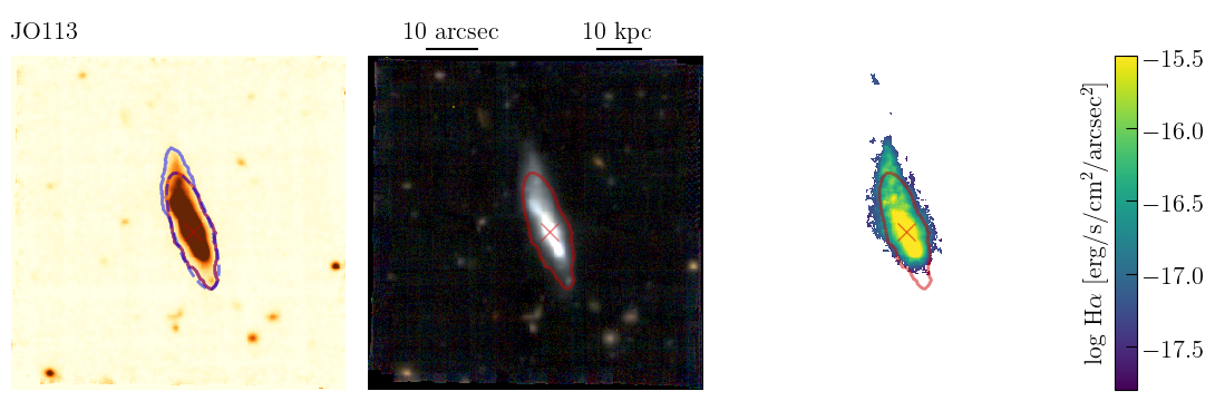
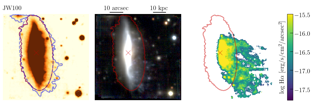
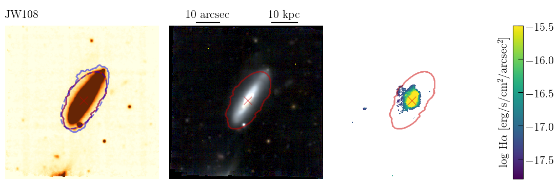
Figure 1: From left to right: (i) the continuum emission in the H$\alpha$ region; (ii) an RGB image obtained from $g-$, $r-$, and $i-$band images derived from the MUSE datacube; ; (iii) the H$\alpha$ emission of three galaxies at different stripping stages: JO113 (moderate stripping), JW100 (jellyfish galaxy), and JW108 (truncated disc or post stripping). The blue line is the isophote corresponding to a continuum surface brightness 1$\sigma$ above the background level; the dashed line is the ellipse that better describes the isophote on the undisturbed side of the galaxy and the red line is the resulting line that we used to define the galaxy main body. The same figure for all galaxies is available at http://web.oapd.inaf.it/gasp/inandout.

3.2 Stellar mass and star formation rates

As in Vulcani et al. (2018), we define the stellar mass of the galaxy main body $M_{\star}$ as the sum of the stellar mass computed with SINOPSIS for each spaxel within the galaxy main body mask. The resulting values are listed in Table 1 and shown in Fig. 2; they range between $6\times 10^{8}$ and $3\times 10^{11}M_{\sun}$. We note that besides SOS 114372 (Merluzzi et al., 2013, which is the GASP galaxy JO147) all other jellyfish galaxies studied in the literature before GASP have stellar masses below $3\times 10^{10}M_{\sun}$ (see the literature review in Poggianti et al. 2019a).

To investigate the gas ionisation mechanism we used the standard BPT diagrams (Baldwin et al., 1981), based on the [O III]5007/H$\beta$ vs [N II]6583/H$\alpha$ line ratios. Following Poggianti et al. (2017a), we adopted the classification scheme based on the results of Kewley et al. (2001), Kauffmann et al. (2003), and Sharp & Bland-Hawthorn (2010) to separate regions with AGN- and LINER-like from star-forming and composite (star-forming+LINER/AGN) regions. In most galaxies the tails are ionised mainly by massive young stars; extended regions with AGN-like emission are observed in JO135 and JO204 which are likely due to the ionisation cone of the central AGN (Gullieuszik et al., 2017; Poggianti et al., 2017b; Radovich et al., 2019).

The SFR was computed from the H$\alpha$ flux corrected for stellar and dust absorption excluding the regions classified as AGN or LINERS and adopting Kennicutt’s relation for a Chabrier (2003) IMF:

$$\mathrm{SFR}=4.6\times 10^{-42}L_{\mathrm{H}\alpha}.$$ (2)

The total SFR and the SFR in the tails (hereafter $\mathrm{SFR}^{\mathrm{TOT}}$ and $\mathrm{SFR}^{\mathrm{OUT}}$, respectively) for all galaxies considered in this paper are listed in Table 1.

Table 1: GASP galaxies used in this work

ID	RA	DEC	cluster	$\sigma_{\mathrm{cl}}$	log$M_{\star}$	$z$	$\mathrm{SFR}^{\mathrm{TOT}}$	$\mathrm{SFR}^{\mathrm{OUT}}$	$r_{\mathrm{cl}}/R_{200}$	$v/\sigma_{\mathrm{cl}}$	JC
	(J2000)	(J2000)		(km/s)			($M_{\sun}\,\mathrm{yr}^{-1}$)	($M_{\sun}\,\mathrm{yr}^{-1}$)
JO5	10:41:20.38	-08:53:45.6	A1069	542	10.27	0.0648	1.350	0.031	1.72	0.26	3
JO10	00:57:41.61	-01:18:44.0	A119	952	10.76	0.0471	3.083	0.000	0.50	0.81	1
JO13	00:55:39.68	-00:52:36.0	A119	952	9.82	0.0479	1.546	0.002	0.57	1.05	4
JO17	01:08:35.33	01:56:37.0	A147	387	10.16	0.0451	0.847	0.000	1.05	0.28	1
JO23	01:08:08.10	-15:30:41.8	A151	771	9.67	0.0551	0.298	0.000	0.45	0.67	1

Note. — This table is published in its entirety in the machine-readable format. A portion is shown here for guidance regarding its form and content.

Note. — Columns are: 1) GASP ID number from Poggianti et al. (2016); 2) and 3) Equatorial coordinate of the galaxy centre; 4) host cluster; 5) velocity dispersion of the host cluster; 6) logarithm of the galaxy stellar mass (in solar masses); 7) galaxy redshift; 8) total SFR; 9) SFR in the tails; 10) projected distance from the cluster centre in units of $R_{200}$; 11) line of sight velocity of the galaxy with respect to the cluster mean in units of the cluster velocity dispersion; 12) Jellyfish Class (JC) from Poggianti et al. (2016);

4 Observational Results

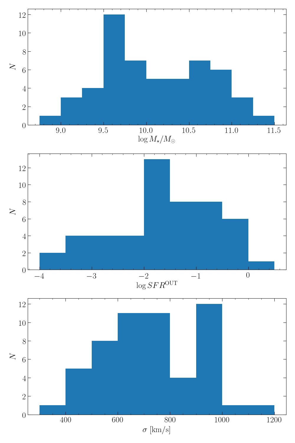
Figure 2: Distribution of the stellar mass (upper panel), SFR in the tails (central panel) and velocity dispersion of the host cluster (lower panel) for the sample galaxies.

Figure 2 shows the distributions of galaxy stellar masses, measured $\mathrm{SFR}^{\mathrm{OUT}}$, and host cluster velocity dispersion. We are sampling galaxies with a wide range of stellar masses, from less than $10^{9}$ to $10^{11.5}M_{\sun}$, hosted in low- and high-mass clusters, with a velocity dispersion from 400 to more than 1000 km s^-1. The SFRs we measured in the tails show a wide variation, reaching values up to more than $1M_{\sun}\,\mathrm{yr}^{-1}$. The decreasing number of galaxies with low $\mathrm{SFR}^{\mathrm{OUT}}$ is likely strongly affected by incompleteness, due to observational effects and/or selection biases.

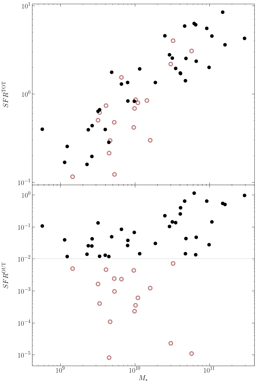
Figure 3: Total SFR (upper panel) and SFR in the tails (lower panel) as a function of the galaxy stellar mass. Red circles shows galaxies with SFR in the tail smaller than $10^{-2}M_{\sun}\,\mathrm{yr}^{-1}$.

The correlation between $\mathrm{SFR}^{\mathrm{TOT}}$ and galaxy stellar mass is shown in the upper panel in Fig. 3; a detailed analysis of this correlation is presented in Vulcani et al. (2018), which demonstrates a statistically significant enhancement of the SFR in both the discs and the tails of GASP ram-pressure stripped galaxies compared to undisturbed galaxies. The lower panel in Fig. 3 shows the relation between the SFR in the tails and the galaxy stellar mass. We define as galaxies with a significant SFR in the stripped tails those with a SFR outside the mask defined in the previous section larger than $10^{-2}M_{\sun}\,\mathrm{yr}^{-1}$; these are shown as black filled symbols in Fig. 3 and do not show a clear and well defined correlation between the SFR in the tail and the stellar mass. All galaxies with $M<10^{10}M_{\sun}$ are forming stars in the tails at a rate $\lesssim 0.1M_{\sun}\,\mathrm{yr}^{-1}$, while only among the most massive galaxies we observe SFR in the tails above this value and up to $1.6M_{\sun}\mathrm{yr}^{-1}$. In addition we found galaxies with low SFR in the tail (open red circles in the lower panel of Fig. 3) at all masses below $10^{11}M_{\sun}$.

The value of the observed $\mathrm{SFR}^{\mathrm{OUT}}$ is expected to depend on many different factors: (i) the total amount of gas available for forming stars; (ii) the efficiency of RPS which, in turn depends on the strength of the ram pressure and on the galaxy anchoring force (see Sect. 5); (iii) the star formation efficiency in the tails, which, in principle, can be different from the one in the galaxy main body. In the following, we use large number of ram-pressure stripped galaxies in the GASP sample to search for general trends.

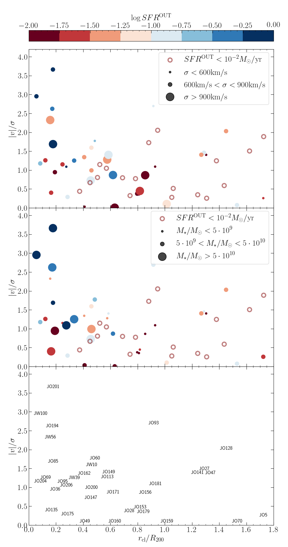
Figure 4: In the two upper panels we plot the phase-space diagram for galaxies with marginal or no star formation in the tails ($\mathrm{SFR}^{\mathrm{OUT}}<10^{-2}M_{\sun}/\textrm{yr}$) as red circles. All other galaxies are colour coded according to the SFR in the tail, as shown in the upper bar. In the upper panel, the point size indicates the host cluster velocity dispersion, in the lower panel the galaxy stellar mass. The bottom panel shows the names of the galaxies with $\mathrm{SFR}^{\mathrm{OUT}}\geq 10^{-2}M_{\sun}/\textrm{yr}$ at the points positions.

The position versus velocity phase-space diagram is an extremely useful tool to investigate environmental effects on the evolution of galaxies in clusters and it has been effectively used by Jaffé et al. (2018) to correlate the stripping stage of GASP galaxies with their orbital histories. The projected phase-space diagram of all our target galaxies is shown in Fig. 4; all galaxies with marginal ($<10^{-2}\rm M_{\odot}yr^{-1}$, empty red circles) SFR in the tails are found at relatively large projected distances ($r_{\textrm{cl}}>0.3R_{200}$). Among these, those at high speed are most likely being accreted (therefore have not been strongly stripped yet), while those at lower speed statistically have spent already more time in the cluster ($>2$Gyr) and probably have little gas left. However, projection effects can blend these two populations. Instead, galaxies with a conspicuous SFR in the tails are preferentially found in the inner cluster regions ($r_{cl}/R_{200}<0.6$) moving at high speed ($|v|>\sigma$) in the ICM (see the colourbar), which suggests they are on first infall into the cluster, on preferentially radial orbits. Figure 4 shows that in the most massive clusters (those with large velocity dispersion shown with the largest symbols in the upper panel in Fig. 4) it is possible to find galaxies with a significant amount of SF in the tail also at relatively large distance from the cluster centre (up to $\sim 0.5-0.6R_{200}$ and/or moving at not extreme velocities ($v/\sigma_{\mathrm{cl}}\lesssim 1.5$).

Galaxies moving at high speed ($|v|>2\sigma_{\mathrm{cl}}$) in the innermost cluster regions ($r_{\mathrm{cl}}<0.5R_{200}$) –the region of the phase-space diagram where the maximum effect of RPS is expected– that have a large SFR in the tails ($\log\mathrm{SFR}^{\mathrm{OUT}}>-0.25$) are all massive and are hosted in low mass clusters (large and small symbols in the lower and upper panel of Fig. 4, respectively). In these galaxies, therefore, the internal anchoring force is stronger due to the gravitational potential of the galaxy itself, and the expected ram-pressure is not so extreme due to the low-mass cluster environment. These galaxies should be the ones able to retain a significant fraction of their gas all the way until they reach the central regions of the cluster. If they were less massive, or within a more massive cluster, they would have been totally stripped before they reached short clustercentric distances. Their value of $\mathrm{SFR}^{\mathrm{OUT}}$ needs to be explained taking into account, therefore, all the parameters cited above.

Three of the four galaxies with $\mathrm{SFR}^{\mathrm{OUT}}<10^{-2}M_{\sun}\,\mathrm{yr}^{-1}$ that are found within $r_{\mathrm{cl}}<0.5R_{200}$ have truncated H$\alpha$ discs, namely JO10, JO23, and JW108. These galaxies likely developed tails at some point in the past that are now completely stripped. The only other GASP galaxy with a truncated disc is JO36. This galaxy has a $\mathrm{SFR}^{\mathrm{OUT}}=0.014M_{\sun}\,\mathrm{yr}^{-1}$, barely above the threshold we adopted, and indeed it lies in the same region of Fig. 4 as the other truncated discs (see Table 1) and has a similarly low $\mathrm{SFR}^{\mathrm{OUT}}$. We note that JO36 is likely undergoing also a gravitational interaction by a fly-by or a close encounter with another galaxy in the cluster which may have stripped part of the gas and hence increased the $\mathrm{SFR}^{\mathrm{OUT}}$ (Fritz et al., 2017). Although its very difficult to isolate back-splashing galaxies in the phase-space due to projection effects, these truncated-disc galaxies are good candidates (see also Yoon et al. 2017)

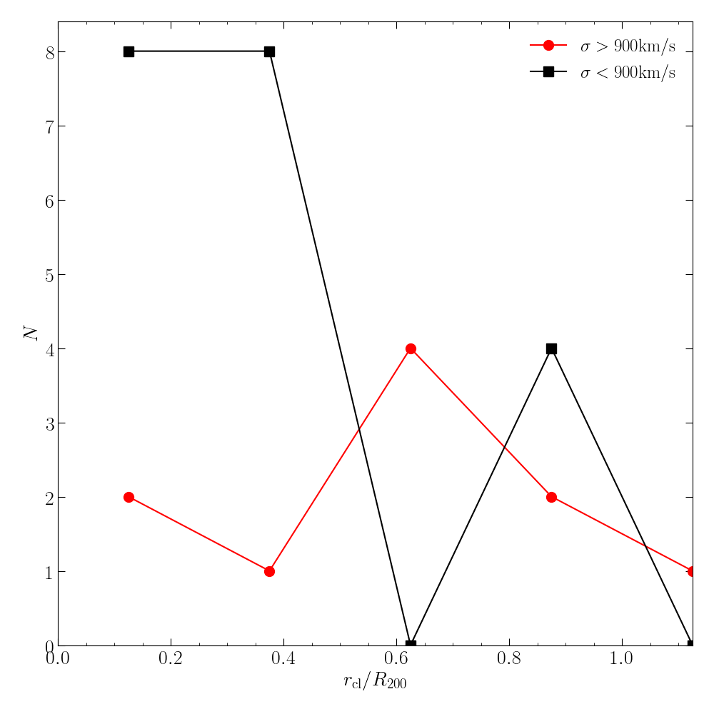
Figure 5: Radial distribution of galaxies with $\mathrm{SFR}^{\mathrm{OUT}}>10^{-2}M_{\sun}\,\mathrm{yr}^{-1}$.

Only a few galaxies with a significant $\mathrm{SFR}^{\mathrm{OUT}}$ ($>10^{-2}M_{\sun}\,\mathrm{yr}^{-1}$) are hosted in the central regions ($r_{\mathrm{cl}}<0.5R_{200})$ of very massive clusters while the majority of them belong to intermediate and low-mass environments. A direct evidence of this is shown in Fig. 5: while the radial distribution of galaxies with $\mathrm{SFR}^{\mathrm{OUT}}>10^{-2}M_{\sun}$ hosted in clusters with $\sigma_{\mathrm{cl}}<900\mathrm{km}\,\mathrm{s}^{-1}$ increases toward the central regions, the distribution of galaxies in clusters with $\sigma_{\mathrm{cl}}>900\mathrm{km}\,\mathrm{s}^{-1}$ is flat at $r_{\mathrm{cl}}\lesssim 0.6R_{200}$. Since the amount of SF in the tails is intimately linked to the gas stripping efficiency, this may be an indication that RPS occurs preferentially at intermediate clustercentric radii in massive clusters and at lower radii in intermediate and low-mass clusters. One of the 2 galaxies in the inner regions of massive clusters is JO85; this is a lopsided galaxy that is very likely undergoing nearly edge-on stripping, that is substantially less efficient than face-on stripping (see for example the simulations in Roediger et al. 2014); this would explain why a substantial fraction of the gas was not stripped during the infall.

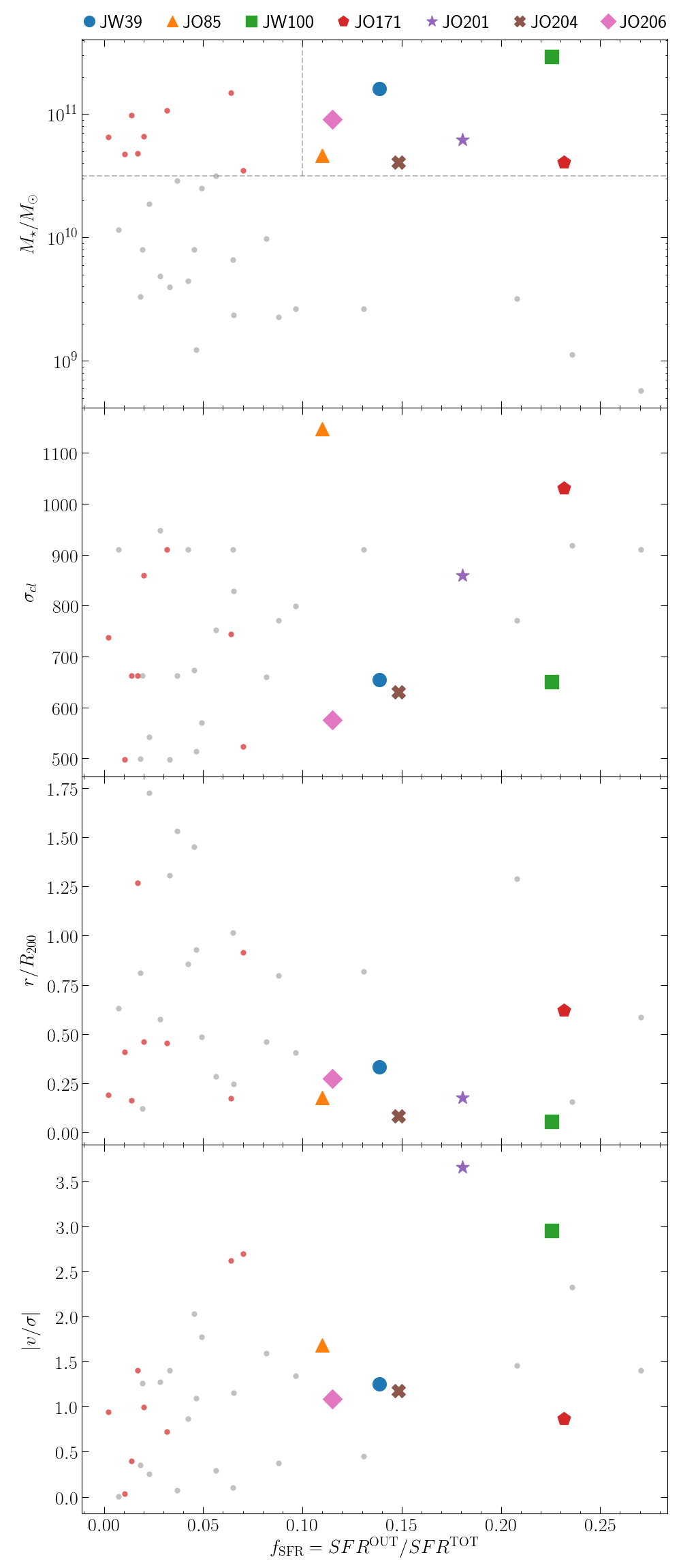
Figure 6: Fraction of SFR in the tails as a function of –from top to bottom panels– the disc stellar mass, the host cluster velocity dispersion, the clustercentric distance and the galaxy radial velocity. Small grey symbols are galaxies with $M_{\star}<10^{10.5}M_{\sun}$; red symbols are for galaxies more massive than this limit and a fraction of SFR in the tail smaller than 10%. Large symbols are massive galaxies with more then 10% of SFR in the tail; names of individual galaxies are given in the legend at the top.

The upper panel in Fig. 6 shows the fraction of SFR in the tail $\mathrm{SFR}^{\mathrm{OUT}}/\mathrm{SFR}^{\mathrm{TOT}}$ ($f_{\mathrm{SFR}}$ thereinafter) as a function of the stellar mass (only for galaxies with $\mathrm{SFR}^{\mathrm{OUT}}>10^{-2}M_{\sun}\mathrm{yr}^{-1}$). As already pointed out, the gravitational potential is much stronger in high-mass galaxies and consequently the anchoring force is stronger than in low-mass galaxies. We see that among the most massive galaxies ($\log M_{\star}/M_{\sun}>10.5$) there are 7 galaxies with a substantial fraction of SFR in the tail, $f_{\mathrm{SFR}}>10\%$. The ram-pressure acting on these galaxies should hence be particularly intense to overcome the anchoring force and strip the gas.

In the lower panels in Fig. 6 we show $f_{\mathrm{SFR}}$ as a function of the main observable quantities regulating the ram-pressure intensity, namely the cluster velocity dispersion (a proxy for the cluster mass, thus related to the ICM density), the clustercentric distance and the peculiar velocity within the ICM normalised by the cluster velocity dispersion. Let us consider the 7 massive galaxies with very high $f_{\mathrm{SFR}}$ values. JW100 is the most massive galaxy in the GASP sample and it is hosted in a relatively low-mass cluster, but it is moving at very high speed and it is very close to the cluster centre, where the ICM is denser. JO85 and JO171 are hosted in two of the most massive clusters ($\sigma_{\mathrm{cl}}>1000\mathrm{km}\,\mathrm{s}^{-1}$), while JO201 is moving at extremely high speed in the ICM of a relatively massive cluster. Finally, JO204, JO206 and JW39 are very close to the centre of their host cluster centre and moving at quite high speed. All these seven galaxies are in exceptional conditions regarding at least one the main parameters regulating the ram-pressure intensity. We note that, besides JO201, all other six galaxies have a tail of stripped gas with a long extension on the plane of the sky, indicating that the component on the plane of the sky of the velocity of the galaxies in the ICM is dominant with respect to the one along the line of sight; the measured radial velocity is therefore a lower limit of their actual speed. Five of these galaxies are studied in detail in dedicated papers ( JW100, Poggianti et al. 2019b; JO171, Moretti et al. 2018c; JO201, Bellhouse et al. 2017, 2019; JO204, Gullieuszik et al. 2017; JO206, Poggianti et al. 2017a).

To summarise, in this section we have described the star formation occurring in the tails of ram-pressure stripped galaxies in terms of both the properties of the galaxies and of the host cluster. We found general trends, but the interplay between all the parameters involved in defining the actual value of $\mathrm{SFR}^{\mathrm{OUT}}$ is complex and all of them must be taken into account. To better understand this scenario we developed an analytical model based on Gunn & Gott (1972) prescriptions aimed at providing an estimate of $\mathrm{SFR}^{\mathrm{OUT}}$ as a function of a limited number of relatively easily measurable quantities.

5 The analytical model

This section presents our analytical approach based on Gunn & Gott (1972) prescriptions to evaluate the fraction of star formation in the tail of ram-pressure stripped galaxies and following the work presented in Jaffé et al. (2018), with a formulation similar to Smith et al. (2012) and Owers et al. (2019).

The ram-pressure on a galaxy moving at a speed $v$ in an ICM with density $\rho$ is

$$P_{\mathrm{RAM}}=\rho v^{2}$$ (3)

The gas within a galaxy will be stripped when $P_{\mathrm{RAM}}$ overcomes the galaxy’s anchoring force $\Pi$ which can be modelled assuming the form:

$$\Pi=2\pi G\Sigma_{\star}\Sigma_{g}$$ (4)

where $G$ is the gravitational constant, $\Sigma_{g}$ and $\Sigma_{\star}$ are the surface density profiles of the gas and stellar discs, respectively. We assumed an exponential profile for both of them:

$$\Sigma_{\star}= \frac{M_{d,\star}}{2\pi R_{d,\star}^{2}}\,e^{-r/R_{d,\star}}$$ (5)

$$\Sigma_{g}= \frac{M_{d,g}}{2\pi R_{d,g}^{2}}\,e^{-r/R_{d,g}}$$ (6)

where $M_{d,g}$ and $M_{d,\star}$ are the mass, and $R_{d,g}$ and $R_{d,\star}$ are the scale lengths of the gas and stellar discs.

We also assumed that:

• galaxies are disc dominated, we therefore defined $M_{\star}\equiv M_{d,\star}$;

• the gas-to-stellar scale length ratio is 1.7, as in Jaffé et al. (2018); this corresponds to the ratio between the H I and optical radius of non-H I-deficient galaxies in Virgo cluster (Cayatte et al., 1994). In the following, the stellar disc scale length will be referred to as $R_{d}$.

We define the truncation radius $r_{t}$ as the distance from the galaxy centre where $\Pi=P_{\mathrm{RAM}}$. At radii larger than $r_{t}$ ram pressure overcomes the anchoring force and the gas is stripped. If we call $f_{\mathrm{gas}}=M_{d,g}/M_{\star}$ the gas mass fraction, we have:

$$\begin{split}\rho v^{2}=&2\pi G\cdot\frac{M_{\star}}{2\pi R_{d}^{2}}e^{-r_{t}/R_{d}}\cdot\frac{f_{\mathrm{gas}}M_{\star}}{2\pi\,1.7^{2}R_{d}^{2}}e^{-r_{t}/(1.7R_{d})}\\ =&\frac{f_{\mathrm{gas}}GM_{\star}^{2}}{2\pi 1.7^{2}R_{d}^{4}}e^{-2.7r_{t}/(1.7R_{d})}\end{split}$$ (7)

Taking the logarithm of both sides of this equation yields

$$\ln(\rho\,v^{2})=\ln\frac{f_{\mathrm{gas}}GM_{\star}^{2}}{2\pi 1.7^{2}R_{d}^{4}}-\frac{2.7r_{t}}{1.7R_{d}}$$ (8)

and hence we obtain

$$\frac{r_{t}}{R_{d}}=\frac{1.7}{2.7}\left[\ln\frac{f_{\mathrm{gas}}GM_{\star}^{2}}{2\pi 1.7^{2}R_{d}^{4}}-\ln(\rho v^{2})\right]$$ (9)

The fraction of remaining gas mass in the galaxy can be calculated by integrating the mass distribution of an exponential disc assuming that all gas outside the truncation disc is stripped and lost. If we call $M_{g}$ the total gas mass, $M_{g}^{\mathrm{IN}}$ the gas mass within $r_{t}$, $M_{g}^{\mathrm{OUT}}$ the mass of the (stripped) gas outside $r_{t}$, we have

$$\frac{M_{g}^{\mathrm{IN}}}{M_{g}}=\frac{\int_{0}^{r_{t}}r\Sigma_{g}\mathrm{d}r}{\int_{0}^{\infty}r\Sigma_{g}\mathrm{d}r}=1-\left[e^{-r_{t}/R_{d,g}}\left(\frac{r_{t}}{R_{d,g}}+1\right)\right]$$ (10)

$$\frac{M_{g}^{\mathrm{IN}}}{M_{g}}=1-\frac{M_{g}^{\mathrm{OUT}}}{M_{g}}$$ (11)

therefore, if we call $f_{M}$ the mass fraction of stripped gas –relative to the total mass– we have:

$$f_{M}=\frac{M_{g}^{\mathrm{OUT}}}{M_{g}}=e^{-r_{t}/(1.7R_{d})}\left(\frac{r_{t}}{1.7R_{d}}+1\right)$$ (12)

Using $r_{t}/R_{d}$ from Eq. 9 in Eq. 12, we have obtained an expression for the fraction of the stripped gas mass as a function of (i) the ICM density $\rho$, (ii) the galaxy gas mass fraction $f_{gas}$, (iii) the galaxy disc scale-length $R_{d}$, (iv) the velocity of the galaxy in the ICM $v$, and (v) the galaxy stellar mass $M_{\star}$. The first one of the above quantities can be expressed as a function of the cluster velocity dispersion $\sigma_{\mathrm{cl}}$ and the clustercentric distance of the galaxy in units of $R_{200}$, while (ii) and (iii) can be derived with some approximation from the galaxy stellar mass $M_{\star}$ under the assumptions described below.

The ICM density $\rho$ is calculated assuming a $\beta$ model:

$$\rho=\rho_{0}\left[1+\left(\frac{r_{\mathrm{cl}}}{R_{c}}\right)^{2}\right]^{-3\beta/2}$$ (13)

where $\rho_{0}$ is the gas density at the centre of the cluster, $R_{c}$ is the cluster core radius, and $r_{\mathrm{cl}}$ is the distance of the galaxy from the cluster centre. We linearly interpolated the values in Table 1 from Jaffé et al. (2018), taking into account the model revision described in Jaffé et al. (2019) to get an expression of $\rho_{0}$ and $R_{c}$ (in units of $R_{200}$) as a function of the cluster velocity dispersion $\sigma_{\mathrm{cl}}$:

$$\rho_{0}=-3.686\times 10^{-3}\sigma_{\mathrm{cl}}+6.200$$ (14)

$$R_{c}/R_{200}=6.738\times 10^{-5}\sigma_{\mathrm{cl}}-3.157\times 10^{-2}$$ (15)

with $\sigma_{\mathrm{cl}}$ in km/s and $\rho_{0}$ in $10^{-23}$ kg/m³. We assumed $\beta=0.5$ for all clusters. We therefore defined $\rho(r)$ as a function of $\sigma_{\mathrm{cl}}$ and the distance from the cluster centre in units of $R_{200}$.

$$\begin{split}\rho=&(-3.686\times 10^{-3}\sigma_{\mathrm{cl}}+6.200)\;\times\\ &\left[1+\left(\frac{r_{\mathrm{cl}}/R_{200}}{6.738\times 10^{-5}\sigma_{\mathrm{cl}}-3.157\times 10^{-2}}\right)^{2}\right]^{-0.75}\end{split}$$ (16)

Following Jaffé et al. (2018), we can express $f_{\mathrm{gas}}$ as a function of the galaxy mass; using the results of Popping et al. (2014) –obtained considering both H I and H₂– we adopted the following quadratic relation:

$$f_{\mathrm{gas}}=0.158\,(\log M_{\star}/M_{\sun})^{2}-3.548\,\log M_{\star}/M_{\sun}+19.964$$ (17)

We lastly assume the scaling relation between the stellar disc scale-length and the stellar mass of galaxies from Wu (2018):

$$\log R_{d}=0.321\times\log\left(M_{\star}/M_{\sun}\right)+0.343$$ (18)

with $R_{d}$ in kpc.

As a sanity check, in Fig. 7 we compare the $r_{t}$ computed by using Eq. 9 (with $R_{d}$ from Eq. 18) with the value estimated from our MUSE data; this was defined as the maximum extension of the H$\alpha$ emission along the galaxy major axis. The overall agreement between the observed $r_{t}$ and the value obtained by our model is satisfactory and supports the reliability of our modeling. The scatter in Fig. 7 originates both from projection effects in the derivation of the observed stripping radius, as well as the caveats inherent to the simple modelization. Figure 11 in the Appendix shows examples of the the computed $r_{t}$ compared with the H$\alpha$ distribution for galaxies with extended tails.

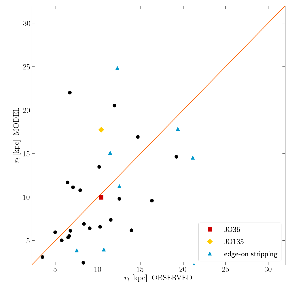
Figure 7: The truncation radius $r_{t}$ computed using the model described in Sect. 5 compared with the value estimated from our observations. The diagonal line is the 1:1 relation. Symbols are as in Fig.9

To conclude, using Eq. 9 and Eq. 12, and the above mentioned assumptions, we can compute the mass fraction of stripped gas $f_{M}$ as a function of cluster velocity dispersion $\sigma_{\mathrm{cl}}$, galaxy peculiar velocity $v$, clustercentric distance $r_{\mathrm{cl}}/R_{200}$, and stellar mass $M_{\star}$. A general view of the results obtained from the analytical model is presented in Fig. 8. At fixed values of all other parameters, the fraction of the stripped gas mass $f_{M}$ decreases for galaxies of increasing stellar mass; the slope of each curve is however rather shallow, indicating that the galaxy mass is not a driving parameter for the fraction of stripped gas. The increase of $f_{M}$ at increasing galaxy speed and host cluster mass due to the stronger ram-pressure is shown by the different sets of lines; the two panels show two different test cases for galaxies located at different clustercentric distances, to highlight the effect of the increased ram-pressure in the inner regions of the clusters on $f_{M}$.

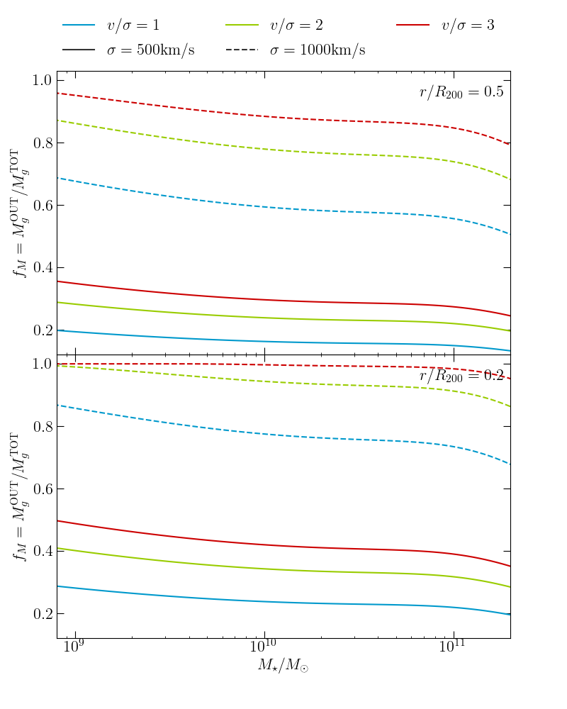
Figure 8: The two panels show the computed fraction of the gas mass stripped by ram-pressure as a function of the stellar mass for galaxies. As shown on the legend at the top of the figure, solid and dashed lines show the case for galaxies infalling into clusters of different velocity dispersion ($\sigma_{\mathrm{cl}}$) while the line colours indicate the value of the galaxy velocity (in units of $\sigma$) in the ICM. In the lower and in the upper panel we plot the values obtained for galaxies located respectively at 0.2 and 0.5 $R_{200}$ from the host cluster centre.

z

We now want to estimate the fraction of star formation which is in the tail from the gas stripped fraction. This will depend on the star formation efficiency, i.e. the amount of stars formed per unit of gas mass, and whether this varies from the disk to the tails. If the star formation efficiency were constant throughout the galaxy (in particular if there were no variations between the disc and the tails), then the fraction of SFR in the tail $f_{\mathrm{SFR}}$ would be equal to the mass fraction of the stripped gas $f_{M}$:

$$f_{M}=\kappa f_{\mathrm{SFR}}=\kappa\frac{\mathrm{SFR}^{\mathrm{OUT}}}{\mathrm{SFR}^{\mathrm{TOT}}}$$ (19)

with $\kappa=1$.

A constant $\kappa=1$ is a useful simplification, although observations find that the SFE decreases as a function of galaxy radius (e.g. Yim et al. 2014), so would be lower in the outer regions where gas is more likely to be removed. Indeed, molecular gas observations of stripped tails have suggested that the star formation efficiency is lower in the tails than in the disks (Jáchym et al., 2014, 2017; Verdugo et al., 2015; Moretti et al., 2018b, 2020a). Using Fig. 6 from Moretti et al. (2018b), based on CO(2-1) APEX observations of four GASP galaxies, we estimate that the difference in star formation efficiency is a factor of $\sim 4$. This is also confirmed by a recent analysis of ALMA data (Moretti et al., 2020b). In addition, by combining the results of our APEX and ALMA observations with H I measurements from JVLA of JO206 (Ramatsoku et al., 2019) we find that the total star formation efficiency (star formation per unit of molecular+neutral gas mass) is lower in the tail than in the disk by a factor 5.4.

In Fig. 9 we compare the $f_{M}$ computed with our model with the observed $f_{\mathrm{SFR}}$ values for galaxies with $\mathrm{SFR}^{\mathrm{OUT}}>10^{-2}M_{\sun}\,\mathrm{yr}^{-1}$. The data-points are clearly not distributed on the $f_{M}=f_{\mathrm{SFR}}$ relation, and the mean value of $\kappa$ (see Eq. 19) that we obtain from our data –excluding post-stripping and edge-on stripping galaxies– is 5.3 (median value 4.5), in striking agreement with the difference in star formation efficiency between tails and disks.

Thus, we observe a correlation between the observed SFR fraction in the tails and the expected mass fraction of the stripped gas based on our model; the relation between these two is compatible with the star formation efficiency measured from the GASP gas studies.

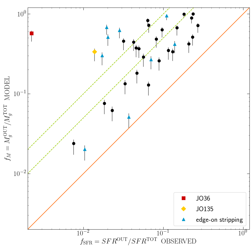
Figure 9: The stripped mass fraction computed with our model is plotted against the observed values of the SFR fraction in the tails of stripped galaxies (see text). Galaxies that are likely undergoing edge-on stripping are shown with triangles. Two galaxies, namely JO36 and JO135 are shown with different symbols and are discussed separately in the text. The solid line, shown for comparison, corresponds to $\kappa=1$ in Eq. 19 (the 1:1 relation), while the two dashed lines correspond to $\kappa=$5 and 10.

The scatter around this relation is large, and in the following we discuss some caveats that must be taken into consideration to properly interpret this result.

• As already noted in Jaffé et al. (2018), our approach likely overestimates RPS: galaxy models assume a pure disc profile and this may under-estimate the anchoring force by neglecting the contribution of the dark matter halo and bulge. The fraction of the stripped gas mass would then be over-estimated, shifting upwards the data-points in Fig. 9.

• Our analytical results refer to the case of galaxies falling nearly face-on into the ICM; in other cases, the ram-pressure would be lower than what is obtained assuming Gunn & Gott (1972) prescriptions. Consequently, our model is expected to overestimate the mass of stripped gas in the case of edge-on stripping. Not all edge-on stripped galaxies (blue triangles), however, lie above the median in Figure 8.

• A fraction of the stripped gas may be completely mixed with the ICM and/or a fraction of the ionised gas emission may be below the MUSE detection limit. Therefore, the gas in the stripped tail at the moment we observe it may be just a fraction of the gas ever stripped and the computed $f_{M}$ would over-estimate the observed $f_{\mathrm{SFR}}$. This effect is clearly more important for galaxies in a late stage of stripping, or even more for post-stripping galaxies. JO36 has a small tail and a truncated H$\alpha$ disc (see Fritz et al. 2017 for a detailed study of JO36); for this galaxy (red square in 9) in fact we measured a very low fraction of SFR in the tail ($<$1%) while our model predicts a consistent fraction of stripped gas. The most plausible scenario is therefore that most of the gas stripped from the galaxy is already lost and dispersed in the ICM and just a very minor fraction of it is close to the galaxy and in dense regions still able to form stars. The other 3 GASP galaxies with truncated H$\alpha$ disc (JO10, JO23, and JW108) are not included in Fig. 9 because they have $\mathrm{SFR}^{\mathrm{OUT}}<10^{-2}M_{\sun}\,\mathrm{yr}^{-1}$ and they would be placed in Fig. 9 even more to the left than JO36.

  In Fig. 9 we also note another outlier that lies in the upper-left region of the diagram. It is JO135 (shown as a yellow diamond). This massive galaxy has a rather long tail of ionised gas but we measure a low SFR in the tail ($\mathrm{SFR}^{\mathrm{OUT}}=0.03M_{\sun}\,\mathrm{yr}^{-1}$, $f_{\mathrm{SFR}}\sim 1\%$). This is likely due to the fact that part of the gas in its tail is ionised by the radiation from the central AGN (Poggianti et al., 2017b; Radovich et al., 2019) and this was consequently not considered in the computation of the total SFR in the tail. The measured $\mathrm{SFR}^{\mathrm{OUT}}$ could therefore be substantially under-estimated.

• Our results are affected by projection effects; both the measured radial velocity and the clustercentric distance component underestimate the 3D values. This induces opposite effects on the computed ram-pressure (an under-estimated speed implies an under-estimated ram-pressure while an under-estimated distance implies an over-estimated ram-pressure). To evaluate the impact of projection effects on our results and on the dispersion of the data-points in Fig. 9, we re-computed $f_{M}$ for each galaxy assuming a velocity $2\times$ the measured radial velocity and then assuming a clustercentric distance $2\times$ the measured component on the plane of the sky. The two resulting values for each galaxy are shown by the vertical bars in Fig. 9. We conclude that overall the distribution of the data-points is not significantly affected by projection effects.

Finally, we emphasise that our model is based on many approximations and strong assumptions and was developed to provide a description of general trends. We assumed a general relation to describe the gas distribution without any assumption on the spatial distribution of the different gas phases. In general, observations of undisturbed galaxies show that molecular gas dominates in the inner regions and atomic gas in the outer ones (see e.g. Bigiel & Blitz, 2012). Our assumptions are compatible with the total gas scale length found by Bigiel & Blitz (2012) (see footnote 1); further investigation of this will be carried out using data from our ongoing multi-wavelength observing campaign. This will probe atomic and molecular gas in GASP galaxies with a resolution similar to the one we obtained for ionised gas with MUSE and will allow us to investigate in detail the spatially resolved SFE. Fig. 9 shows that our approach provides a quite satisfactory description of the observations, which in turn implies that, albeit with a large scatter, the four quantities that can be derived from observations (cluster velocity dispersion, galaxy velocity, clustercentric distance and mass) can provide a crude approximation of the fraction of star formation taking place in the tails. This also suggests that additional factors (e.g. link with cluster substructure/merging) are probably only second order effects.

6 intracluster light

In this section, the GASP results will be used to obtain a rough estimate of the total contribution from RPS to the intracluster light. An implicit assumption we will make is that the stars formed in the regions which we call tails will be lost from the galaxy at some stage and will become part of the intracluster component, thus neglecting the fact that some of these stars might still be bound to the galaxy and eventually join the disk. Our generous choice of the disk boundaries should limit this effect, but this caveat should be kept in mind.

We used the complete catalogue of candidate RPS galaxies published from Poggianti et al. (2016), from which the GASP target galaxies were selected. This catalogue was compiled using data from WINGS (Fasano et al., 2006) and OmegaWINGS (Gullieuszik et al., 2015), which are two complete surveys of X-ray selected clusters in the redshift range 0.04-0.07 at galactic latitude $|l|>20^{\circ}$ (66% of the sky). The selection of GASP candidates was carried out trying to span the whole range of parameters of interest, in particular galaxy mass, cluster mass and JClass (degree of asymmetry in the optical galaxy morphology, see Poggianti et al., 2016). We can therefore assume that GASP provides a reasonably representative snapshot of the population of ram-pressure stripped galaxies in the nearby Universe.

Table 2: Integrated values of the SFR for all galaxies grouped according to the JClass classification from Poggianti et al. (2016). Columns are: 1) JClass; 2) total number of galaxies in Poggianti et al. (2016); 3) number of galaxies in this paper; 4) average of the $\mathrm{SFR}^{\mathrm{OUT}}$ in the tail for galaxies in this paper; 5) total $\mathrm{SFR}^{\mathrm{OUT}}$ multiplied by the number of galaxies in Poggianti et al. (2016).

JClass	$n^{\mathrm{P16}}_{\mathrm{JC}}$	$n_{\mathrm{JC}}$	$\mathrm{SFR}^{\mathrm{OUT}}_{\mathrm{JC}}$	$\mathrm{SFR}^{\mathrm{OUT}}_{\mathrm{JC,TOT}}$
			$M_{\sun}\mathrm{yr}^{-1}$	$M_{\sun}\mathrm{yr}^{-1}$
1	131	13	0.031	4.11
2	115	10	0.012	1.41
3	67	11	0.035	2.37
4	21	12	0.089	1.88
5	10	8	0.595	5.95

To estimate the total amount of SFR in the tails of ram-pressure stripped galaxies we grouped the GASP galaxies according to the JClass; for each of the five groups we computed the average tail SFR6 that we call $\mathrm{SFR}^{\mathrm{OUT}}_{\mathrm{JC}}$. We then multiplied the resulting values for the number of galaxies in each JClass in Poggianti et al. (2016). Results are reported in Table 2. The total SFR for all ram-pressure stripped galaxies is the sum of the five values obtained for each JClass:

$$\mathrm{SFR}^{\mathrm{OUT}}_{\mathrm{TOT}}=\sum_{\mathrm{JC}=1}^{5}n^{\mathrm{P16}}_{\mathrm{JC}}\times\mathrm{SFR}^{\mathrm{OUT}}_{\mathrm{JC}}=\sum_{\mathrm{JC}=1}^{5}\mathrm{SFR}^{\mathrm{OUT}}_{\mathrm{JC,TOT}}$$ (20)

The resulting estimate for the integrated SFR in the tails of all ram-pressure stripped galaxies in these clusters is $15.72M_{\sun}\mathrm{yr}^{-1}$. Since the total number of clusters hosting ram-pressure stripping candidates in Poggianti et al. (2016) is 71, the average value per cluster is $0.22M_{\sun}\mathrm{yr}^{-1}$.

We note that the sky coverage of our target clusters in not uniform, as the FoV of WINGS and OmegaWINGS imaging is $30^{\prime}$ and $1^{\circ}$, respectively, and only a fraction of clusters has OmegaWINGS observations. To assess the possible impact of this on our analysis, we repeated our computation by selecting GASP and Poggianti et al. (2016) data only for galaxies in clusters with OmegaWINGS observations. In this case we found an average SFR per cluster of $0.25M_{\sun}\mathrm{yr}^{-1}$. This value is not significantly different from the one we obtain from our complete dataset, showing that the different sky coverage of the WINGS/OmegaWINGS target clusters does not affect our conclusions.

We can now use our GASP results on the SFR in the tails to trace back in time the contribution of ram-pressure stripping to the ICL. This can be computed assuming that the average value of the SFR in the tail per cluster is simply proportional to the infalling rate of galaxies in the cluster. We consider the infall of galaxies at $z\leq 1$, an epoch at which the evolution of the ICM is negligible and WINGS/OMEGAWINGS clusters should have already developed their dense and hot ICM able to induce RPS (Leauthaud et al., 2010; Bulbul et al., 2019).

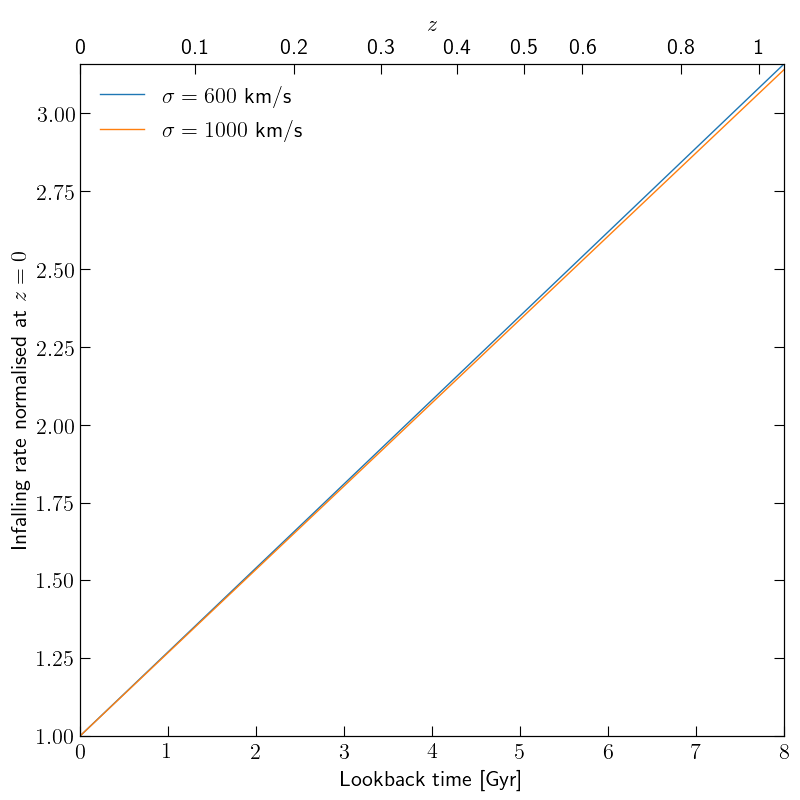
Figure 10: Infalling rates normalised to the value at $z=0$ for the two model clusters.

We compute the rate of galaxies infalling into galaxy clusters as a function of lookback time by using the semi-analytic model of Henriques et al. (2015). This model is based on implementing analytic equations which simplify the baryonic physics of galaxy formation on the background of a cosmological Millennium N-body simulation (Springel et al., 2005) which has been recalibrated to be consistent with the cosmological model favoured by the Planck satellite (Planck Collaboration et al., 2014). This model assumes a $\sigma_{8}$ = 0.829, and has cosmological parameters closer to those used in our observations than the original Millennium simulation. The small differences in our adopted $\Omega_{M}$ and $\Omega_{\Lambda}$ do not have appreciable differences in the infall histories recovered.

This semi-analytic model is the most recent version of the Munich galaxy formation model, and was particularly focused on tweaking the analytics implementations to correctly reproduce star formation rates, colours and stellar masses of galaxies. While semi-analytic models can vary in their underlying equations, and therefore in their predictions, in this work we only use the predictions for the stellar masses of galaxies at any particular redshift which are most robustly predicted by different models. Indeed, we recover similar results when using a recent version of the Durham galaxy formation model for the same cosmology.

To take into account the possible influence of the cluster halo mass on the infalling rate, we calculated it for two different halo masses: one corresponding to a low-mass cluster ($\sim 3\times 10^{14}M_{\sun}$) and one to high-mass one ($\sim 2\times 10^{15}M_{\sun}$). Therefore, from the Henriques et al. models we select all halos having a velocity dispersion between 500 and 600 km/s and 800 and 1200 km/s, respectively. We then selected, within each halo, every galaxy with a stellar mass M${}_{\mathrm{stellar}}>$ M_stellar,cut and track it through the simulation to find the time at which it was first accreted into the final cluster. The results were examined for M_stellar,cut = 10¹⁰ and 10⁹ and in both total halo mass bins. To exclude from our analysis galaxies that were pre-processed before being accreted into the halo, we considered for our calculations only objects at first infall. This selection was accomplished by ignoring galaxies which were in a dark matter halo with a velocity dispersion of $<$ 500 km/s at the time of their accretion into the main cluster.

The cumulative fractions of galaxies infalling into the two simulated clusters as a function of lookback time were fitted using a second-order polynomial. The infalling rates are obtained as the derivative of the cumulative fraction of infalling galaxies and therefore result to be a linear function of the look-back time. As expected the infalling rates are larger for the high-mass halo. However, we are only interested in the evolution of the infall rate, not its absolute value, so we can normalize it to the infalling rate at z=0, which roughly represents the epoch of the GASP observations. After this normalization, the evolution of the infall rate is almost independent of the cluster velocity dispersion bin or the stellar mass cut. As this normalised infalling rate is essentially driven by the underlying cosmology, the mass independence is not surprising. The results are shown in Fig. 10.

The computed normalized infalling rates, simply multiplied by our GASP estimate of the average total SFR in the tails per cluster ($0.22M_{\sun}\mathrm{yr}^{-1}$, see above) gives our estimate of the evolution of the contribution of ram-pressure stripping to the ICM per average cluster. At $z=1$ it results to be $\approx$3 times the value at $z=0$. By integrating our results we estimate a total value of $\approx 4\times 10^{9}M_{\sun}$ of stars formed per cluster in the ICM from ram-pressure stripped gas since z$\sim 1$. We stress that this value has been derived for a set of clusters with an average value of velocity dispersion of $750\mathrm{km}\,\mathrm{s}^{-1}$ at $z\sim 0$ (Poggianti et al., 2016), while this number could be higher for more massive clusters.

The contribution of ram-pressure stripping in shaping the ICL is still extremely uncertain. Adami et al. (2016) concluded that RPS is the most plausible process generating the ICL sources; other studies proposed different mechanisms, such as tidal stripping of massive (DeMaio et al., 2018; Montes & Trujillo, 2018) or low-mass (Morishita et al., 2017) galaxies. Direct measurements of the ICL are challenging, mostly because it is extremely difficult to disentangle the diffuse component of the ICL from the contribution of the galaxies and in particular from the Brightest Cluster Galaxy (BCG). A clear understanding of the origin of the ICL is also hampered by the uncertainties on the properties of the mass, the age and metallicity of the ICL’s stellar component. Most of the literature studies of the ICL are in fact based on broad-band imaging data and photometric SED fitting. Only a few spectroscopic studies have been published so far and it is not possible to draw final conclusions on the properties and the origin of the ICL (see e.g. Coccato et al. 2011; Melnick et al. 2012 based on long-slit/MOS spectroscopy and Adami et al. 2016 based on MUSE IFU spectroscopy). More spectroscopic observations are still required to further investigate the physical processes driving the formation and the evolution of the ICL. The exceptional spatial resolution, FoV and sensitivity of MUSE could most likely play a primary role.

7 Summary and conclusions

As part of the GASP project based on an ESO Large Programme with MUSE, this paper focuses on the SFR in the tails of cluster galaxies underging ram-pressure stripping. By considering all GASP cluster galaxies –excluding merging and tidally interacting systems – we used a sample of 54 galaxies; our sample covers a wide parameter space in terms of galaxy stellar mass, between less than $10^{9}$ and $10^{11.5}M_{\sun}$, and host cluster mass/velocity dispersion, between 400 to more than 1000 $\mathrm{km}\,\mathrm{s}^{-1}$. We defined a method to conservatively define a mask to disentangle the ram-pressure stripped gas tail from the galaxy main body. We computed the SFR from the H$\alpha$ emission by using BPT diagnostic diagrams to exclude the gas not ionised by SF. We used our measurements to study how the SFR in the tail depends on the properties of the galaxy and of its host cluster. We found that there is not a single dominant parameter driving the observed value of the $\mathrm{SFR}^{\mathrm{OUT}}$; the mass of the galaxy, its position and velocity in the host cluster and all the parameters defining the distribution of the ICM density are all to be considered to properly account for the $\mathrm{SFR}^{\mathrm{OUT}}$. However we found general trends that are here summarized.

All galaxies with marginal $\mathrm{SFR}^{\mathrm{OUT}}$ are found at relatively large distances from the host cluster center. Some of these are galaxies at the first infall in the cluster that are being accreted and therefore had not been stripped yet.

All the galaxies with large $\mathrm{SFR}^{\mathrm{OUT}}$ ($>0.25M_{\sun}\,\mathrm{yr}^{-1}$) that are moving at large speed in the innermost regions of the clusters are massive and hosted in low-mass clusters; only under these conditions the gravitational potential can contrast the extreme ram-pressure stripping that would otherwise strip most of the gas before these galaxies could reach the inner cluster regions

RPS occurs preferentially at intermediate clustercentric distance in massive clusters and at lower distances in intermediate and low-mass clusters. This is because galaxies are nearly completely stripped when they reach the dense region of high-mass clusters.

To provide a method to predict the amount of SFR in the tails using observable quantities, based on our observational results. We developed a simple analytical approach based on ram-pressure prescriptions from Gunn & Gott (1972); we aimed at deriving the fraction of stripped mass as a function of galaxy and clusters parameters that can be easily obtained from observations. Following other literature work (e.g. Smith et al., 2012; Owers et al., 2019; Jaffé et al., 2018), we made standard assumptions and we adopted scaling relations for (i) the galaxy gas fraction and disc scale-length as a function of the galactic stellar mass and (ii) the ICM central density and core radius as a function of the cluster velocity dispersion. As a result, we obtained an analytic expression for the mass fraction of stripped gas as a function of four parameters: the cluster velocity dispersion, the galaxy stellar mass, its clustercentric distance and speed in the ICM. To assess the reliability of our model, we compared the computed truncation radius –the galactocentric distance at which the ram-pressure equals the gravitational anchoring force– with the ionised gas emission maps obtained from MUSE observations; the remarkable agreement is a strong indication that our assumptions provides a reasonable description of the properties of the galaxies and their host cluster.

A direct comparison of the fraction of stripped mass computed with our model with the observed fraction of SFR in the tails shows a very good agreement (albeit with a large scatter) between the two quantities if the total (molecular+neutral) star-formation efficiency is lower in the tail than in the disk by a factor $\sim 5$, in excellent agreement with the efficiency derived from our ongoing CO and H I observing campaign with APEX, ALMA and JVLA (Moretti et al., 2018b; Ramatsoku et al., 2019; Moretti et al., 2020b).

We used the values of the SFR in the tails of stripped gas to estimate the contribution of RPS to the ICL. By statistically correcting our GASP measurements using the whole GASP parent candidate catalog from Poggianti et al. (2016), we found that the average SFR for all ram-pressure stripped galaxies per cluster is $0.22M_{\sun}\,\mathrm{yr}^{-1}$. We finally used this result to extrapolate the contribution to the ICL at different look-back times, by assuming that it is proportional to the number of galaxies at first infall into the cluster. The infalling rate was computed using the cosmological semi-analytical model by Henriques et al. (2015) based on the Millenium N-body Simulation. We estimated a total average value per cluster of $\approx 4\times 10^{9}M_{\sun}$ of stars formed in the ICM from ram-pressure stripped gas since $z=1$. This estimate can be used to evaluate the contribution of RPS in shaping the ICL and therefore is a valuable contribution to the still open debate about the physical processes driving the formation and the evolution of the ICL.

Appendix A Truncation radius

Figure 11 shows examples of the the computed $r_{t}$ compared with the H$\alpha$ distribution. Only galaxies with extended tails were considered, excluding cases of edge-on stripping.

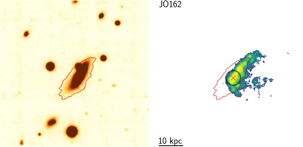
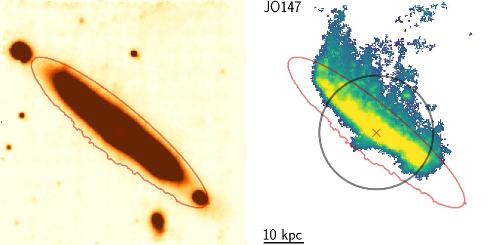
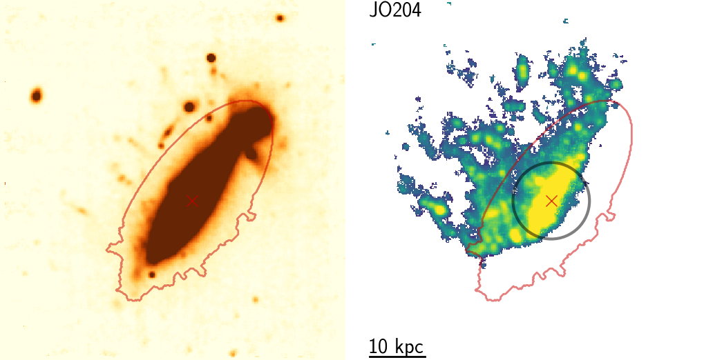
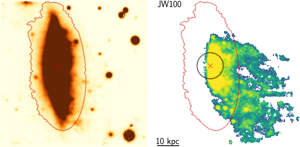
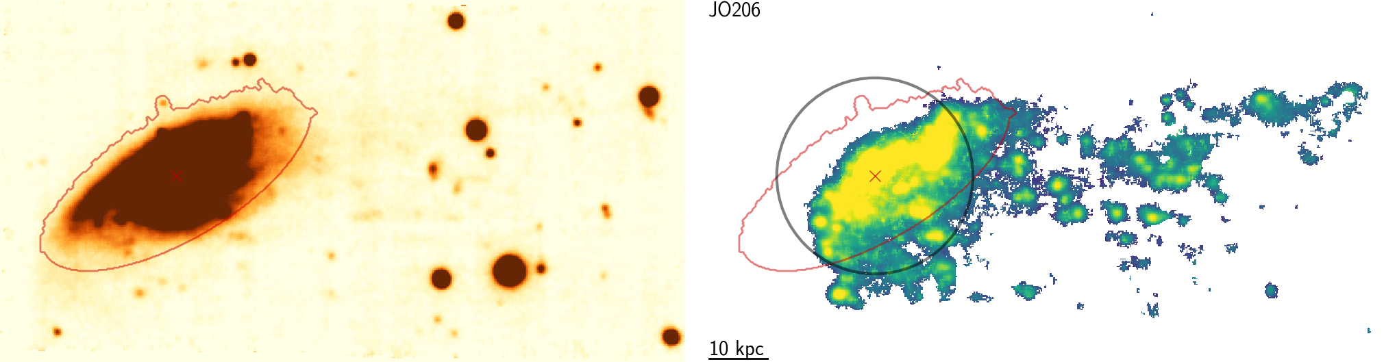
Figure 11: Continuum emission map, H$\alpha$ emission, and the contour used to define the galaxy main body as in Fig. 1 for jellyfish galaxies with extended tails. The blue circle show the truncation radius $r_{t}$ computed using the model described in Sect. 5.

References

- Abramson et al. (2011) Abramson, A., Kenney, J. D. P., Crowl, H. H., et al. 2011, AJ, 141, 164
- Adami et al. (2016) Adami, C., Pompei, E., Sadibekova, T., et al. 2016, A&A, 592, A7
- Bacon et al. (2010) Bacon, R., Accardo, M., Adjali, L., et al. 2010, in Proc. SPIE, Vol. 7735, Ground-based and Airborne Instrumentation for Astronomy III, 773508
- Baldwin et al. (1981) Baldwin, J. A., Phillips, M. M., & Terlevich, R. 1981, PASP, 93, 5
- Bellhouse et al. (2017) Bellhouse, C., Jaffé, Y. L., Hau, G. K. T., et al. 2017, ApJ, 844, 49
- Bellhouse et al. (2019) Bellhouse, C., Jaffé, Y. L., McGee, S. L., et al. 2019, MNRAS, 485, 1157
- Bigiel & Blitz (2012) Bigiel, F., & Blitz, L. 2012, ApJ, 756, 183
- Biviano et al. (2017) Biviano, A., Moretti, A., Paccagnella, A., et al. 2017, A&A, 607, A81
- Boissier et al. (2012) Boissier, S., Boselli, A., Duc, P. A., et al. 2012, A&A, 545, A142
- Boselli & Gavazzi (2006) Boselli, A., & Gavazzi, G. 2006, PASP, 118, 517
- Boselli et al. (2016) Boselli, A., Cuillandre, J. C., Fossati, M., et al. 2016, A&A, 587, A68
- Bulbul et al. (2019) Bulbul, E., Chiu, I. N., Mohr, J. J., et al. 2019, ApJ, 871, 50
- Calvi et al. (2011) Calvi, R., Poggianti, B. M., & Vulcani, B. 2011, MNRAS, 416, 727
- Cappellari & Emsellem (2004) Cappellari, M., & Emsellem, E. 2004, PASP, 116, 138
- Cardelli et al. (1989) Cardelli, J. A., Clayton, G. C., & Mathis, J. S. 1989, ApJ, 345, 245
- Cayatte et al. (1994) Cayatte, V., Kotanyi, C., Balkowski, C., & van Gorkom, J. H. 1994, AJ, 107, 1003
- Chabrier (2003) Chabrier, G. 2003, PASP, 115, 763
- Chung et al. (2007) Chung, A., van Gorkom, J. H., Kenney, J. D. P., & Vollmer, B. 2007, ApJ, 659, L115
- Coccato et al. (2011) Coccato, L., Gerhard, O., Arnaboldi, M., & Ventimiglia, G. 2011, A&A, 533, A138
- Contini et al. (2018) Contini, E., Yi, S. K., & Kang, X. 2018, MNRAS, 479, 932
- DeMaio et al. (2018) DeMaio, T., Gonzalez, A. H., Zabludoff, A., et al. 2018, MNRAS, 474, 3009
- Ebeling et al. (2014) Ebeling, H., Stephenson, L. N., & Edge, A. C. 2014, ApJ, 781, L40
- Fasano et al. (2006) Fasano, G., Marmo, C., Varela, J., et al. 2006, A&A, 445, 805
- Fossati et al. (2016) Fossati, M., Fumagalli, M., Boselli, A., et al. 2016, MNRAS, 455, 2028
- Fritz et al. (2017) Fritz, J., Moretti, A., Gullieuszik, M., et al. 2017, ApJ, 848, 132
- Fumagalli et al. (2014) Fumagalli, M., Fossati, M., Hau, G. K. T., et al. 2014, MNRAS, 445, 4335
- Gavazzi (1989) Gavazzi, G. 1989, ApJ, 346, 59
- George et al. (2018) George, K., Poggianti, B. M., Gullieuszik, M., et al. 2018, MNRAS, 479, 4126
- Giallongo et al. (2014) Giallongo, E., Menci, N., Grazian, A., et al. 2014, ApJ, 781, 24
- Giovanelli & Haynes (1985) Giovanelli, R., & Haynes, M. P. 1985, ApJ, 292, 404
- Guglielmo et al. (2015) Guglielmo, V., Poggianti, B. M., Moretti, A., et al. 2015, MNRAS, 450, 2749
- Gullieuszik et al. (2015) Gullieuszik, M., Poggianti, B., Fasano, G., et al. 2015, A&A, 581, A41
- Gullieuszik et al. (2017) Gullieuszik, M., Poggianti, B. M., Moretti, A., et al. 2017, ApJ, 846, 27
- Gunn & Gott (1972) Gunn, J. E., & Gott, III, J. R. 1972, ApJ, 176, 1
- Henriques et al. (2015) Henriques, B. M. B., White, S. D. M., Thomas, P. A., et al. 2015, MNRAS, 451, 2663
- Hester et al. (2010) Hester, J. A., Seibert, M., Neill, J. D., et al. 2010, ApJ, 716, L14
- Jáchym et al. (2014) Jáchym, P., Combes, F., Cortese, L., Sun, M., & Kenney, J. D. P. 2014, ApJ, 792, 11
- Jáchym et al. (2017) Jáchym, P., Sun, M., Kenney, J. D. P., et al. 2017, ApJ, 839, 114
- Jáchym et al. (2019) Jáchym, P., Kenney, J. D. P., Sun, M., et al. 2019, ApJ, 883, 145
- Jaffé et al. (2015) Jaffé, Y. L., Smith, R., Candlish, G. N., et al. 2015, MNRAS, 448, 1715
- Jaffé et al. (2018) Jaffé, Y. L., Poggianti, B. M., Moretti, A., et al. 2018, MNRAS, 476, 4753
- Jaffé et al. (2019) —. 2019, MNRAS, 482, 3454
- Kapferer et al. (2009) Kapferer, W., Sluka, C., Schindler, S., Ferrari, C., & Ziegler, B. 2009, A&A, 499, 87
- Kauffmann et al. (2003) Kauffmann, G., Heckman, T. M., Tremonti, C., et al. 2003, MNRAS, 346, 1055
- Kenney et al. (2014) Kenney, J. D. P., Geha, M., Jáchym, P., et al. 2014, ApJ, 780, 119
- Kenney et al. (2004) Kenney, J. D. P., van Gorkom, J. H., & Vollmer, B. 2004, AJ, 127, 3361
- Kewley et al. (2001) Kewley, L. J., Dopita, M. A., Sutherland, R. S., Heisler, C. A., & Trevena, J. 2001, ApJ, 556, 121
- Leauthaud et al. (2010) Leauthaud, A., Finoguenov, A., Kneib, J.-P., et al. 2010, ApJ, 709, 97
- Leroy et al. (2008) Leroy, A. K., Walter, F., Brinks, E., et al. 2008, AJ, 136, 2782
- McPartland et al. (2016) McPartland, C., Ebeling, H., Roediger, E., & Blumenthal, K. 2016, MNRAS, 455, 2994
- Melnick et al. (2012) Melnick, J., Giraud, E., Toledo, I., Selman, F., & Quintana, H. 2012, MNRAS, 427, 850
- Merluzzi et al. (2013) Merluzzi, P., Busarello, G., Dopita, M. A., et al. 2013, MNRAS, 429, 1747
- Montes & Trujillo (2018) Montes, M., & Trujillo, I. 2018, MNRAS, 474, 917
- Moretti et al. (2017) Moretti, A., Gullieuszik, M., Poggianti, B., et al. 2017, A&A, 599, A81
- Moretti et al. (2018a) Moretti, A., Paladino, R., Poggianti, B. M., et al. 2018a, MNRAS, 480, 2508
- Moretti et al. (2018b) —. 2018b, MNRAS, 480, 2508
- Moretti et al. (2018c) Moretti, A., Poggianti, B. M., Gullieuszik, M., et al. 2018c, MNRAS, 475, 4055
- Moretti et al. (2020a) Moretti, A., Paladino, R., Poggianti, B. M., et al. 2020a, ApJ, 889, 9
- Moretti et al. (2020b) —. 2020b, arXiv e-prints, arXiv:2006.13612
- Morishita et al. (2017) Morishita, T., Abramson, L. E., Treu, T., et al. 2017, ApJ, 846, 139
- Munari et al. (2013) Munari, E., Biviano, A., Borgani, S., Murante, G., & Fabjan, D. 2013, MNRAS, 430, 2638
- Owers et al. (2019) Owers, M. S., Hudson, M. J., Oman, K. A., et al. 2019, ApJ, 873, 52
- Planck Collaboration et al. (2014) Planck Collaboration, Ade, P. A. R., Aghanim, N., et al. 2014, A&A, 571, A16
- Poggianti et al. (2016) Poggianti, B. M., Fasano, G., Omizzolo, A., et al. 2016, AJ, 151, 78
- Poggianti et al. (2017a) Poggianti, B. M., Moretti, A., Gullieuszik, M., et al. 2017a, ApJ, 844, 48
- Poggianti et al. (2017b) Poggianti, B. M., Jaffé, Y. L., Moretti, A., et al. 2017b, Nature, 548, 304
- Poggianti et al. (2019a) Poggianti, B. M., Gullieuszik, M., Tonnesen, S., et al. 2019a, MNRAS, 482, 4466
- Poggianti et al. (2019b) Poggianti, B. M., Ignesti, A., Gitti, M., et al. 2019b, ApJ, 887, 155
- Popping et al. (2014) Popping, G., Somerville, R. S., & Trager, S. C. 2014, MNRAS, 442, 2398
- Radovich et al. (2019) Radovich, M., Poggianti, B., Jaffé, Y. L., et al. 2019, MNRAS, 486, 486
- Ramatsoku et al. (2019) Ramatsoku, M., Serra, P., Poggianti, B. M., et al. 2019, MNRAS, 487, 4580
- Roediger et al. (2014) Roediger, E., Bruggen, M., Owers, M. S., Ebeling, H., & Sun, M. 2014, MNRAS, 443, L114
- Schlafly & Finkbeiner (2011) Schlafly, E. F., & Finkbeiner, D. P. 2011, ApJ, 737, 103
- Sharp & Bland-Hawthorn (2010) Sharp, R. G., & Bland-Hawthorn, J. 2010, ApJ, 711, 818
- Smith et al. (2012) Smith, R., Fellhauer, M., & Assmann, P. 2012, MNRAS, 420, 1990
- Smith et al. (2010) Smith, R. J., Lucey, J. R., Hammer, D., et al. 2010, MNRAS, 408, 1417
- Springel et al. (2005) Springel, V., White, S. D. M., Jenkins, A., et al. 2005, Nature, 435, 629
- Sun et al. (2006) Sun, M., Jones, C., Forman, W., et al. 2006, ApJ, 637, L81
- The Astropy Collaboration et al. (2018) The Astropy Collaboration, Price-Whelan, A. M., Sipőcz, B. M., et al. 2018, ArXiv e-prints, arXiv:1801.02634
- Tonnesen & Bryan (2012) Tonnesen, S., & Bryan, G. L. 2012, MNRAS, 422, 1609
- Verdugo et al. (2015) Verdugo, C., Combes, F., Dasyra, K., Salomé, P., & Braine, J. 2015, A&A, 582, A6
- Vollmer et al. (2009) Vollmer, B., Soida, M., Chung, A., et al. 2009, A&A, 496, 669
- Vulcani et al. (2018) Vulcani, B., Poggianti, B. M., Gullieuszik, M., et al. 2018, ApJ, 866, L25
- Wu (2018) Wu, P.-F. 2018, MNRAS, 473, 5468
- Yagi et al. (2010) Yagi, M., Yoshida, M., Komiyama, Y., et al. 2010, AJ, 140, 1814
- Yim et al. (2014) Yim, K., Wong, T., Xue, R., et al. 2014, AJ, 148, 127
- Yoon et al. (2017) Yoon, H., Chung, A., Smith, R., & Jaffé, Y. L. 2017, ApJ, 838, 81
- Yoshida et al. (2004) Yoshida, M., Ohyama, Y., Iye, M., et al. 2004, AJ, 127, 90