Non-Markovian decoherence dynamics of the hybrid quantum system
with a cavity strongly coupling to a spin ensemble: a master equation approach

Abstract

Based on the recent experiments on the hybrid quantum system of a superconducting microwave cavity coupling strongly to an inhomogeneous broadening spin ensemble under an external driving field, we use the exact master equation approach to investigate its non-Markovian decoherence dynamics. Here the spin ensemble is made by negatively charged nitrogen-vacancy (NV) defects in diamond. Our exact master equation theory for open systems depicts the experimental decoherence results and reveals the mechanism how the decoherence induced by the inhomogeneous broadening is suppressed in the strong-coupling regime. Moreover, we show how the spectral hole burning generates localized states to further suppress the cavity decoherence. We also investigate the two-time correlations in this system to further show how quantum fluctuations manifest quantum memory.

I Introduction

Cavity QED systems have become promising quantum devices for individual quantum system controlling and for quantum information storage, processing and transmission Haroche2006 . Such systems are also attracted great interest in the study of the fundamental quantum theory of open systems and the measurement-induced decoherence dynamics Carmichael93 . Cavity QED is the study of interaction between matters and quantized electromagnetic fields. Since the early 1980s, the investigation of cavity QED has moved towards strong coupling systems with high quality factor cavities Kimble03 . The strong coupling cavity QED has been experimentally realized with a multitude of physical systems including Rydberg atoms in microwave cavities Haroche96 ; Walther01 , alkali atoms in optical cavities Kimble92 ; Kimble98 ; Kimble04 , and superconducting circuits Girvin04 ; Mooij04 , etc. For certain circumstance, in the strong-coupling regime, decoherence (coherence loss) of photon and atom states can be effectively suppressed in cavity QED and single photon and single atom states can be dynamically manipulated.

Meanwhile, an alternative realization of strong-coupling cavity QED has also been developed with the hybrid quantum systems of large spin or atom ensembles coupled to superconducting microwave cavities Xiang13 , where the collective coupling strength is proportional to the square root of the number of emitters. Also the spin or atomic ensemble plays the role of quantum memories that quantum information can be coherently stored and retrieved at some later time. Such hybrid systems have been realized with various spin ensembles, such as negatively charged nitrogen-vacancy (NV) defects in diamond Majer11 ; Kubo11 , rare-earth spin ensembles Probst13 , and magnons in yttrium iron garnet Huebl13 ; Tabuchi14 , etc. In particular, the NV centers in diamond have the long coherence time even at room temperature, which shows the great potential for quantum information storage. The strong coupling of such spin ensembles with microwave cavities could make coherent transfer of quantum information more feasible.

However, due to the local magnetic dipole-dipole couplings of NV centers constituting the ensemble to residual nitrogen paramagnetic impurities, the resonance line of a large NV electron spin ensemble is inhomogeneously broadened Stanwix10 ; Kurucz11 ; Diniz11 ; Sandner11 . Inhomogeneous spin ensemble broadening could induce decoherence to the cavity system and therefore may limit the performance of the coherent transfer and storage of quantum information. However, in the strong-coupling regime, inhomogeneous broadening induced decoherence may be suppressed upon the width and shape of the inhomogeneous broadening, which is called as ”cavity protection effect” Kurucz11 ; Diniz11 . Recently, Putz et al. have experimentally demonstrated such effect through the real-time dynamics of a superconducting microwave cavity coupled strongly to the spin ensemble of NV centers Putz14 ; Putz17 . By appropriately choosing microwave pulses, they can increase the amplitude of coherent oscillations between the cavity and the spin ensemble. They also used a semi-classical mean field approximation to explain their observation Krimer14 ; Krimer15 . In this paper, we will study the real-time dynamics of such hybrid quantum systems from the dynamics of open quantum systems with the exact master equation approach we developed Tu2008 ; Lei2012 ; Zhang2012 ; Zhang2018 . With this master equation formulation, some new insights of the decoherence dynamics in this hybrid quantum system can be revealed.

The experimental setup Putz14 ; Putz17 of the superconducting microwave cavity coupled strongly to the spin ensemble of NV centers can be described by the Tavis-Cummings model TCmodel . Therefore in this paper, we will start with the Tavis-Cummings model to investigate the decoherence dynamics of cavity QED due to the spin ensemble. Such decoherence dynamics heavily involves non-Markovian memory processes. The Tavis-Cummings model with the spin ensemble at arbitrary temperature cannot be solved exactly. However, the experimental setup enables one to convert the spin ensemble into a bosonic ensemble using the Holstein-Primakoff approximation HP1938 , from which we can derive the exact master equation. Then we can systematically study the non-Markovian dynamics of Tavis-Cummings model using the master equation incorporating an external driving field Lei2012 ; Zhang2012 . We can also addresses rigorously quantum dissipation and thermal fluctuation together to depict the decoherence dynamics. As a result, the non-Markovian decoherence dynamics in this hybrid quantum systems can be understood better. It reveals the mechanism of how the decoherence induced by the inhomogeneous broadening can be suppressed in the strong-coupling regime. Also, we show that the solution of the decoherence suppression by the spectral hole burning is due to the localized bound states (localized modes) between the cavity and the spin ensemble generated by the hole burning spectral density. Localized states are dissipationless as a general property of open quantum systems Zhang2012 . We also use two time-correlation functions to explore quantum memory effect Ali2015 ; Ali2017 ; min-review . It enables us to accurately address the dynamics of the cavity photons in the quantum regime.

The rest of the paper is organized as follows. In Sec. II, we discuss the master equation theory of open quantum systems for the hybrid system studied in this paper. We will briefly discuss the generalized Tavis-Cummings model for the hybrid quantum system consisting of a superconducting microwave cavity coupled strongly to a spin ensemble of NV centers under the control of microwave pulse driving field. With the Holstein-Primakoff approximation to the spin ensemble under the experimental setup, we obtain the exact master equation for the cavity system with the external driving field. We also discuss the physical consequence of the dissipation and fluctuations from the master equation through the comparison with the exact quantum Langevin equation. We further explore how the two-time correlation functions characterize quantum memory. In Sec. III and Sec. IV, we study in detail the decoherence dynamics of the cavity field and compare with the experiment data and other theoretical methods for different setups of the spin ensemble in this hybrid quantum system. We also use the time correlation functions to study quantum memory far from the semiclassical dynamics in Sec. V. In the last, a conclusion is given in Sec. VI.

II Tavis-Cummings model with external driving field and the exact master equation method

The hybrid quantum system consists of a superconducting microwave cavity coupled strongly to the spin ensemble of NV centers and the cavity is driven by an appropriate microwave pulse. This system can be described by a generalized Tavis-Cummings model with the following Hamiltonian,

$$H(t)=\, \hbar\omega_{c}a^{\dagger}a+\big{[}f(t)a^{\dagger}+f^{*}(t)a\big{]}$$

$$+\sum_{k}\big{[}\Delta_{k}\sigma^{z}_{k}+V_{k}a^{\dagger}\sigma^{-}_{k}+V^{*}_{k}\sigma^{+}_{k}a\big{]}$$

$$+\sum_{l}\big{[}\hbar\omega_{l}b^{\dagger}_{l}b_{l}+V_{l}a^{\dagger}b_{l}+V^{*}_{l}b^{\dagger}_{l}a\big{]}.$$ (1)

where the first term describes a single-mode cavity, and $a^{\dagger}$($a$) is the corresponding bosonic creation (annihilation) operator with $\omega_{c}$ being the resonate frequency. The second term describes the microwave pulse driving field $f(t)=\eta(t)\mathrm{e}^{-i\omega_{p}t}$ acting on the cavity with the time-dependent field strength $\eta(t)$ and the phase frequency $\omega_{p}$. The driving pulse is used to control the dynamics of the hybrid system through the cavity. The third term is the Hamiltonian of the spin ensemble of NV centers and its coupling with the cavity, where $\sigma^{z}_{k},\sigma^{\pm}_{k}$ represent the three Pauli matrices for each spin with $\Delta_{k}$ being the corresponding two level energy splitting, and $g_{k}$ is the coupling amplitude. The remaining Hamiltonian describes the cavity leakage into the free space electromagnetic background environment, where $c_{l}^{\dagger}$($c_{l}$) is the creation (annihilation) operator of the photonic mode $l$ with frequency $\omega_{l}$ in the background environment, and $V_{l}$ is the coupling amplitude between the cavity mode and the background environmental mode $l$.

The dynamics of the total systems (the cavity system, the spin ensemble and the free space environmental modes) is given by the total density matrix following the unitary evolution,

$$\rho_{\text{tot}}(t)=U(t,t_{0})\rho_{\text{tot}}(t_{0})U^{\dagger}(t,t_{0}),$$ (2)

where $U(t,t_{0})$=$\mathcal{T}\text{exp}\left(\frac{1}{i\hbar}\int^{t}_{t_{0}}d\tau H(\tau)\right)$ is the time evolution operator of the total system, and ${\cal T}$ is the time-ordering operator. Initially, the cavity system is empty, the spin ensemble and the environment are in the partitioned thermal state, that is, $\rho_{\text{tot}}(t_{0})$=$\rho_{\text{c}}(t_{0})$$\otimes$$\rho_{\text{s}}(t_{0})$$\otimes$$\rho_{\text{e}}(t_{0})$. Indeed, the density matrix of the cavity state $\rho_{\text{c}}(t_{0})$ can be arbitrary, and the others are thermal equilibrium states: $\rho_{\text{s}}(t_{0})$=$\frac{1}{Z_{s}}e^{-\beta_{s}\sum_{k}\Delta_{k}\sigma^{z}_{k}}$ and $\rho_{\text{e}}(t_{0})$=$\frac{1}{Z_{e}}e^{-\beta_{e}\sum_{l}\hbar\omega_{l}b^{\dagger}_{l}b_{l}}$, where $\beta_{s}=1/(kT_{s})$ and $\beta_{e}=1/(kT_{e})$ are the inverse of their initial temperatures which could be the same or different. Immediately after the time $t_{0}$, the cavity, the spin ensemble and the environment evolve into a non-equilibrium state under Eq. (2). Because experimentally one measures the physical observables of the cavity system, such as the cavity field intensity (photon numbers) and photon correlations, we shall focus on the cavity photon state dynamics only, which is determined by the reduced density matrix

$$\rho_{c}(t)=\text{Tr}_{s+e}\big{[}\rho_{\text{tot}}(t)\big{]}$$ (3)

that encompasses all the influences caused by the spin ensemble and the environment after we trace over all all the spin and environmental states.

In the experimental setup Putz14 ; Putz17 , only a small percentage of spins ($\approx\!\!10^{6}$) are excited in comparison with the total spin number ($\approx\!10^{12}$) in the ensemble, which corresponds to the high polarization spin ensemble Kurucz11 . Thus the Holstein-Primakoff approximation HP1938

$$\sigma^{z}_{k}\equiv c^{\dagger}_{k}c_{k}-1/2,~{}~{}\sigma^{+}_{k}\equiv c^{\dagger}_{k}\sqrt{1-c^{\dagger}_{k}c_{k}}\simeq c^{\dagger}_{k}$$ (4)

can be applied to the spin variables, where $c^{\dagger}_{k},c_{k}$ correspond to the creation and annihilation operators of the boson mode $k$. As a result, the Hamiltonian Eq. (5) can be reduced to

$$H=\, \hbar\omega_{c}a^{\dagger}a+\big{[}f(t)a^{\dagger}+f^{*}(t)a\big{]}$$

$$+\sum_{k}\big{[}\Delta_{k}c^{\dagger}_{k}c_{k}+V_{k}a^{\dagger}c_{k}+V^{*}_{k}c^{\dagger}_{k}a\big{]}$$

$$+\sum_{l}\big{[}\hbar\omega_{l}b^{\dagger}_{l}b_{l}+V_{l}a^{\dagger}b_{l}+V^{*}_{l}b^{\dagger}_{l}a\big{]},$$ (5)

with a good accuracy in the comparison with experimental data, as we will show later. Then the dynamics of the hybrid quantum system (the cavity, the spin ensemble and the environment) can be exactly solved. Usually decoherence of photon states due to environmental leakages and atomic absorptions can be treated with constant decay rates (Markov decoherence phenomena) Carmichael93 . For the strong coupling cavity QED system with the spin ensemble, the resonance line of the NV spin ensemble is inhomogeneously broadened so that non-Markovian decoherence dominates the dynamics in this hybrid quantum system. To study the non-Markovian decoherence dynamics of the system, we apply the exact master equation approach developed recently Tu2008 ; Lei2012 ; Zhang2012 ; Zhang2018 , which has been used in many other applications Lei2011 ; Yang2014 ; Lo2015 ; Ali2015 ; Yang2017 ; Yang2018 ; Lai2018 .

Following the standard procedure given in Ref. Lei2012 , after traced over all the spin and environmental states from Eq. (2), we obtain the exact master equation of the reduced density matrix for the cavity system governed by the total Hamiltonian of Eq. (5),

$$\frac{d}{dt}\rho_{c}(t)= \frac{1}{i\hbar}\big{[}\omega^{\prime}_{c}(t,t_{0})a^{\dagger}a{+}f^{\prime*}(t,t_{0})a{+}f^{\prime}(t,t_{0})a^{\dagger},\rho_{c}(t)\big{]}$$

$$+\gamma(t,t_{0})\big{[}2a\rho_{c}(t)a^{\dagger}\!-\!a^{\dagger}a\rho_{c}(t)\!-\!\rho_{c}(t)a^{\dagger}a\big{]}$$

$$+\widetilde{\gamma}(t,t_{0})\big{[}a\rho_{c}(t)a^{\dagger}\!+\!a^{\dagger}\rho_{c}(t)a$$

$$~{}~{}~{}~{}~{}~{}~{}~{}~{}~{}~{}~{}~{}~{}~{}~{}~{}~{}~{}~{}~{}~{}~{}~{}\!-\!a^{\dagger}a\rho_{c}(t)\!-\!\rho_{c}(t)aa^{\dagger}\big{]},$$ (6)

where the first term describes a unitary evolution of cavity photon states, in which the effective cavity frequency $\omega^{\prime}_{c}(t,t_{0})$ and the effective external driving field $f^{\prime*}(t,t_{0})$ have taken into account the renormalized effects nonpturbatively due to the coupling to the spin ensemble. The other two terms in the master equation represent the non-unitary evolution due to the dissipation and fluctuations that are induced completely by the the spin ensemble and the environment. The dissipation and fluctuations are characterized explicitly with the dissipation and fluctuation coefficients, $\gamma(t,t_{0})$ and $\widetilde{\gamma}(t,t_{0})$, respectively. They describe the detailed relaxation of the cavity field and the thermalization between the cavity and the spin ensemble. The most important feature in the above exact master equation is that the time nonlocal renormalized cavity frequency $\omega^{\prime}_{c}(t,t_{0})$, renormalized external driving field $f^{\prime*}(t,t_{0})$, dissipation coefficient $\gamma(t,t_{0})$ and fluctuation coefficient $\widetilde{\gamma}(t,t_{0})$ are determined nonperturbatively by the nonequilibrium Green functions Lei2012 ,

$$i\omega_{c}^{\prime}(t,t_{0})+\gamma(t,t_{0})=-\frac{\dot{u}(t,t_{0})}{u(t,t_{0})},$$ (7a)

$$f^{\prime}(t,t_{0})=i\dot{y}(t,t_{0})-i\left[\frac{\dot{u}(t,t_{0})}{u(t,t_{0})}y(t,t_{0})\right],$$ (7b)

$$\tilde{\gamma}(t,t_{0})=\lim_{\tau\rightarrow t}\frac{\partial{v}(\tau,t)}{\partial\tau}-\left[\frac{\dot{u}(t,t_{0})}{u(t,t_{0})}v(t,t)+\text{c.c}\right],$$ (7c)

where the nonequilibrium Green functions $u(t,t_{0})$, $y(t,t_{0})$ and $v(\tau,t)$ obey the following integro-differential equations

$$\frac{d}{dt}u(t,t_{0})\!+\!i\omega_{c}u(t,t_{0})+\!\!\int^{t}_{t_{0}}\!\!\!d\tau g(t,\tau)u(\tau,t_{0})=0,$$ (8a)

$$\frac{d}{dt}y(t,t_{0})\!+\!i\omega_{c}y(t,t_{0})+\!\!\int^{t}_{t_{0}}\!\!\!d\tau g(t,\tau)y(\tau,t_{0})=\frac{1}{i\hbar}f(t),$$ (8b)

$$\frac{d}{d\tau}v(\tau,t)\!+\!i\omega_{c}v(\tau,t)+\!\!\int^{\tau}_{t_{0}}\!\!\!d\tau^{\prime}g(\tau,\tau^{\prime})v(\tau^{\prime},t)$$

$$~{}~{}~{}~{}~{}~{}~{}~{}~{}~{}~{}~{}~{}~{}~{}~{}~{}~{}~{}~{}~{}~{}~{}~{}=\!\!\int^{t}_{t_{0}}\!\!\!dt^{\prime}\widetilde{g}(\tau,t^{\prime})\bar{u}(t^{\prime},t),~{}~{}(\tau\leq t)$$ (8c)

subjected to the boundary conditions $u(t_{0},t_{0})$=$1$, $y(t_{0},t_{0})$=$0$ and $v(t_{0},t)$=$0$. In Eq. (8), the nonlocal integral kernels, $g(t,\tau)$ and $\widetilde{g}(t,\tau)$, are given as follows,

$$g(t,\tau) =\frac{1}{\hbar^{2}}\!\sum_{k}|V_{k}|^{2}\mathrm{e}^{-i\Delta_{k}(t-\tau)/\hbar}+\frac{1}{\hbar^{2}}\!\sum_{l}|V_{l}|^{2}\mathrm{e}^{-i\omega_{l}(t-\tau)}$$

$$=\sum_{\alpha=s,e}\int_{0}^{\infty}\frac{d\omega}{2\pi}J_{\alpha}(\omega)\mathrm{e}^{-i\omega\left(t-\tau\right)},$$ (9a)

$$\widetilde{g}(t,\tau) =\frac{1}{\hbar^{2}}\!\sum_{k}|V_{k}|^{2}\bar{n}(\Delta_{k}/\hbar,T_{s})\mathrm{e}^{-i\Delta_{k}(t-\tau)/\hbar}$$

$$~{}~{}~{}+\frac{1}{\hbar^{2}}\!\sum_{l}|V_{l}|^{2}\bar{n}(\omega_{l},T_{e})\mathrm{e}^{-i\omega_{l}(t-\tau)}$$

$$=\sum_{\alpha=s,e}\int_{0}^{\infty}\frac{d\omega}{2\pi}J_{\alpha}(\omega)\bar{n}(\omega,T_{\alpha})\mathrm{e}^{-i\omega\left(t-\tau\right)},$$ (9b)

where

$$J_{s}(\omega)=\frac{2\pi}{\hbar^{2}}\sum_{k}|V_{k}|^{2}\delta(\omega-\Delta_{k}/\hbar),$$ (10a)

$$J_{e}(\omega)=\frac{2\pi}{\hbar^{2}}\sum_{l}|V_{l}|^{2}\delta(\omega-\omega_{l})\simeq 2\kappa$$ (10b)

are the spectral densities associated with the spin ensemble or the environment, respectively, and $\bar{n}_{s,e}(\omega,T_{s,e})=1/(e^{\hbar\omega/kT_{s,e}}-1)$ are the corresponding particle distribution function. The frequency-dependence of $J_{s}(\omega)$ depicts the inhomogeneous broadening of the spin ensemble spectrum, and the cavity decay rate $\kappa$ characterizes the cavity leakage effect.

From the above result, we can further simplify the integro-differential equation of $u(t,t_{0})$ as

$$\frac{d}{dt}u(t,t_{0})+ (i\omega_{c}+\kappa)u(t,t_{0})=$$

$$- \!\!\int^{t}_{t_{0}}\!\!\!d\tau\!\!\int_{0}^{\infty}\!\!\frac{d\omega}{2\pi}J_{s}(\omega)\mathrm{e}^{-i\omega\left(t-\tau\right)})u(\tau,t_{0}).$$ (11)

The result shows that without the spin ensemble, the solution of $u(t,t_{0})$ simply describes the spontaneous decay of the cavity field. The last term in Eq. (11) determines the dynamical process of the cavity photons dissipating into the spin ensemble, as will be seen clearer later. Furthermore, because of the boundary conditions $y(t_{0},t_{0})$=$0$ and $v(t_{0},t)$=$0$, Eqs. (8c)-(8b) can be analytically solved in terms of $u(t,t_{0})$ Lei2012 ,

$$y(t,t_{0})=\frac{1}{i\hbar}\int^{t}_{t_{0}}\!\!d\tau u(t,\tau)f(\tau),$$ (12a)

$$v(\tau,t)=\int^{\tau}_{t_{0}}\!\!\!dt_{1}\!\!\int^{t}_{t_{0}}\!\!\!dt_{2}u(\tau,t_{1})\widetilde{g}(t_{1},t_{2})u^{\dagger}(t,t_{2}).$$ (12b)

As we will see later from Eq. (18), $y(t,t_{0})$ is the driving-field-induced cavity field combining with the dissipation effect raised from the spin ensemble and the environment. More precisely speaking, $y(t,t_{0})$ comes from the driving field directly and then decays mainly due to the coupling of the cavity with the spin ensemble. While, the two-time function $v(\tau,t)$ is the correlation associated with the initial state of the spin ensemble and also the free-space environment. If the spin ensemble and the environment can be initially prepared at zero temperature, then $v(\tau,t)=0$. Therefore, $v(\tau,t)$ is the quantum correlation of the cavity photon mixed with thermal fluctuations.

Now, using the exact master equation, we can easily compute the experimentally measured cavity field $\langle a(t)\rangle=\operatorname{Tr}[a\rho_{c}(t)]$ or more precisely the cavity intensity (cavity photon number) $\langle n(t)\rangle=\operatorname{Tr}[a^{\dagger}a\rho_{c}(t)]$:

$$\langle a(t)\rangle= u(t,t_{0})\langle a(t_{0})\rangle+y(t,t_{0}),$$ (13a)

$$\langle n(t)\rangle= |u(t,t_{0})|^{2}\langle a^{\dagger}(t_{0})a(t_{0})\rangle+|y(t,t_{0})|^{2}+v(t,t)$$

$$+[u^{*}(t,t_{0})y(t,t_{0})\langle a^{\dagger}(t_{0})\rangle+{\rm c.c.}]$$ (13b)

The semiclassical method Putz et al. used based on the Volterra integral equation to explain their experimental observations Putz14 ; Putz17 can be equivalently written as

$$\langle n(t)\rangle_{\rm sc}=|\langle a(t)\rangle|^{2}=|u(t,t_{0})\langle a(t_{0})\rangle|^{2}+|y(t,t_{0})|^{2}$$

$$+[u^{*}(t,t_{0})y(t,t_{0})\langle a^{\dagger}(t_{0})\rangle+{\rm c.c.}].$$ (14)

The difference between the full quantum mechanical solution given here and the semiclassical solution in Refs. Putz14 ; Putz17 is the quantum fluctuation

$$\langle n(t)\rangle- \langle n(t)\rangle_{\rm sc}=v(t,t)$$

$$+ |u(t,t_{0})|^{2}(\langle a^{\dagger}(t_{0})a(t_{0})\rangle-\langle a^{\dagger}(t_{0})\rangle\langle a(t_{0})\rangle).$$ (15)

which is negligible in the semiclassical regime (the average photon number $\langle n(t)\rangle\sim 10^{6}$ as was measured in experiments Putz14 ; Putz17 ). However, in the quantum regime where $\langle n(t)\rangle$ is the order of one or less, quantum fluctuations becomes significant and the semiclassical method used in Putz14 ; Putz17 becomes invalid. This effect should become particularly important in the study of quantum memory for quantum information processing, as we will discuss in Sec. V.

For a self-consistency check and also for a clearer physical interpretation to the decoherence dynamics described in the master equation, the above result can also be obtained from the quantum Langevin equation derived from Heisenberg equation of motion. Using the Heisenberg equation of motion and eliminating the variables of the spin ensemble as well as the free-space environmental modes, we have derived the following quantum Langevin equation Yang2014 ; Tan2011 ; Yang2015 ; Yang2017 for the cavity field operator $a(t)$

$$\frac{d}{dt} a(t)+(i\omega_{c}+\kappa)a(t)$$

$$+\!\!\int^{t}_{t_{0}}\!\!d\tau\!\!\int_{0}^{\infty}\!\!\!\frac{d\omega}{2\pi}J_{s}(\omega)\mathrm{e}^{-i\omega\left(t-\tau\right)}a(\tau)=\frac{1}{i\hbar}\big{[}f(t)+\xi(t)\big{]},$$ (16)

where $\xi(t)$ is the noise force induced by the spin ensemble and also the environment:

$$\xi(t)=\!\sum_{k} V_{k}\mathrm{e}^{-i\Delta_{k}(t-t_{0})/\hbar}c_{k}(t_{0})+\!\sum_{l}V_{l}\mathrm{e}^{-i\omega_{l}(t-t_{0})}b_{l}(t_{0}).$$ (17)

Moreover, due to the linearity of Eq. (II), the general solution of the quantum Langevin equation is

$$a(t)=u(t,t_{0})a(t_{0})+y(t,t_{0})+\chi(t,t_{0}),$$ (18)

from which we can find that $u(t,t_{0})$ and $y(t,t_{0})$ are given by Eq. (11)-(12a), and $\chi(t,t_{0})$ is the noise field induced by the noise force $\xi(t)$:

$$\chi(t,t_{0})=\frac{1}{i\hbar}\int^{t}_{t_{0}}d\tau u(t,\tau)\xi(\tau)$$ (19)

It is easy to check that the correlation function $v(t,t)$ of Eq. (12b) obtained in the master equation method is indeed the noise correlation:

$$v(\tau,t)=\langle\chi^{\dagger}(t,t_{0})\chi(\tau,t_{0})\rangle,$$ (20)

at $\tau=t$. Thus, we recover the results from the master equation. These results show that all the time nonlocal parameters in the master equation are fully determined by the cavity’s Green function $u(t,t_{0})$ from Eq. (11). It should be pointed out that it is the convolution integral in Eq. (11) that takes into account all the possible non-Markovian effects of the cavity system interacting with the spin ensemble Zhang2018 .

III Decoherence dynamics of the cavity coupled strongly to the spin ensemble

In the two recent experimental setup by Putz et al. Putz14 ; Putz17 , the superconducting microwave cavity frequency $\omega_{c}$ is set to $2\pi$$\times$$2.69$ GHz, and the main frequency $\omega_{s}$ of the spin spectral density is resonant with the cavity, $\omega_{c}=\omega_{s}$, but has the broadening effect. To reduce the thermal fluctuation effect, the entire experimental setup is cooled down to $T_{s}=25$ mK, which is only about one-fifth of the excitation energy of spins. Besides, spins are surrounded by a Helmholtz coil which supplies a strong magnetic field to modify the spins in a relative ground state. By controlling the strength of the driving pulse, the number of injected photons is manifested to be about or less than $10^{6}$, which is much lower than the total number of spins $\approx$ $10^{12}$ in the cavity so that the Holstein-Primakoff approximation to the spin ensemble becomes applicable. By applying the driving field, the cavity photonic state may be coherently stored and retrieved from the spin ensemble for quantum information processing.

The main difference between Putz14 and Putz17 is the manipulation of the broadening spectral density of the spin ensemble. The spectral density of Eq. (10a) is experimentally fitted as a q-Gaussian spectral density Putz14

$$J_{s}(\omega)=2\pi\Omega^{2}\cdotp C\cdotp\left[1-(1-q)\frac{(\omega-\omega_{s})^{2}}{\Delta^{2}}\right]^{\frac{1}{1-q}},$$ (21)

which is an intermediate form between a Gaussian spectral density and a Lorentzian spectral density with $q=1.39$, where C is its normalization constant, and $\omega_{s}$ is the main frequency of the spin ensemble, $\Delta$ is determined by the full-width at the half maximum of $J_{s}(\omega)$ which is given by $\gamma$=$2\Delta\sqrt{\frac{2^{q}-2}{2q-2}}$=$18.8\pi$ MHz, and the coupling strength $2\Omega$=$2\pi\times 17.2$ MHz represents a strong coupling in Ref. Putz14 . The specific profile of the spectral density $J_{s}(\omega)$ is shown in Fig. 1(a). While the spectral density in the experiment Putz17 is a modification of Eq. (21) as shown in Fig. 1(b), which is made by the spectral hole burning technique, a well-established technique in quantum optics used to turn off the excitations at some specific frequencies in the spin ensemble. Here, the particular frequencies of $\omega_{s}$$\pm$$\frac{\Omega_{R}}{2}$ are burnt out as shown in Fig. 1(b). Besides, in the experiment Putz17 , the full-width at half maximum of the spectral density is changed slightly to $18.2\pi$ MHz, and the coupling strength $\Omega\approx\frac{\Omega_{R}}{2}{=}21.3\pi$ MHz with $\Omega_{R}$ being the Rabi frequency. The cavity decay rate $\kappa/2\pi=0.4$ MHz. Our calculations are all based on these experimental parameter setup.

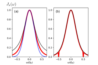
Figure 1: The spectral density of the spin ensemble as a function of the frequency in the unit of $\Omega_{R}$ by a central frequency shifting $\omega-\omega_{s}\rightarrow\omega$. (a) The black, blue and red curves correspond to the spectral densities of a Gaussian form, a Lorentzian form, and the q-Gaussian form of Eq. (21), respectively. (b) The black (thin) curve is the original q-Gaussian form, and the red (thick) curve is modified from the q-Gaussian form by the hole burning technique Putz17 .

The full quantum mechanical description of the hybrid quantum system given in the last section shows that the cavity dissipation or decoherence dynamics is fully determined by the Green function $u(t,t_{0})$ of Eq. (11). Its general solution has been given in Zhang2012 . Explicitly, taking a modified Laplace transformation $U(z)=\int^{\infty}_{t_{0}}u(t,t_{0})\mathrm{e}^{iz(t-t_{0})}dt$ to Eq. (11), we have

$$U(z)=\frac{i}{z-\omega_{c}+i\kappa-\Sigma(z)},$$ (22)

where $\Sigma(z)$ is the self-energy correction,

$$\Sigma(z)=\int^{\infty}_{-\infty}\frac{d\omega}{2\pi}\frac{J_{s}(\omega)}{z-\omega},$$ (23)

and

$$\lim_{z\to\omega\pm i\epsilon}\Sigma(z)=\Delta(\omega)\mp\frac{i}{2}\!J_{s}(\omega).$$ (24)

Here $\Delta(\omega)$=$\sum_{\alpha}\mathcal{P}\int^{\infty}_{-\infty}\frac{d\omega^{\prime}}{2\pi}\frac{J_{\alpha}(\omega^{\prime})}{\omega-\omega{\prime}}$ is the principal value of Eq.(23), which gives the cavity frequency shift due to the spin ensemble. The general solution to $u(t,t_{0})$ is expressed as Zhang2012

$$u(t,t_{0})= \sum_{\omega_{b}}\mathcal{Z}(\omega_{b})\mathrm{e}^{-i\omega_{b}(t-t_{0})}$$

$$+\frac{2}{\pi}\!\int_{-\infty}^{\infty}\!\!d\omega\frac{J_{s}(\omega)\mathrm{e}^{-i\omega(t-t_{0})}}{4\big{[}\omega-\omega_{c}-\Delta(\omega)+i\kappa\big{]}^{2}+J^{2}_{s}(\omega)}.$$ (25)

where the first term is a dissipationless term contributed from localized modes and the residues $\mathcal{Z}_{\omega_{b}}{=}\frac{1}{1-\Sigma^{\prime}(\omega_{s})}$ are the corresponding wave function amplitudes. A localized mode can exist only when the spectrum density has gaps or is a finite band, that is, $\sum_{\alpha}J_{\alpha}(\omega_{b})$=$0$ such that $\omega_{b}{=}\omega_{c}{+}\Delta(\omega_{b})$. The second term of Eq. (III) is a contribution from the branch cut due to the discontinuity of $\Sigma(z)$, so does $U(z)$, across the real axis on the complex space $z$ in the inverse Laplace transformation of Eq. (22). It is shown by Eq. (24). This branch cut induces an non-exponential decay. Both contributions in Eq. (III) are evidences of non-Markovian dynamics in open quantum systems Zhang2012 .

Because the cavity decay rate $\kappa\neq 0$, strictly speaking, no localized mode can exist in this hybrid quantum system. Thus, the solution to $u(t,t_{0})$ is simply given by

$$u(t{-}t_{0})=\frac{2}{\pi}\!\!\int_{-\infty}^{\infty}\!\!\!d\omega\frac{J_{s}(\omega)\mathrm{e}^{-i\omega(t-t_{0})}}{4\big{[}\omega-\omega_{c}-\Delta(\omega)+i\kappa\big{]}^{2}+J^{2}_{s}(\omega)}.$$ (26)

Figure 2 shows the detailed solution of the Green function $u(t,t_{0})$ with the q-Gaussian spectral density Eq. (21) for the spin ensemble. It contains all the decoherence information of the cavity system strongly coupled with the spin ensemble, as shown in Fig. 2(d). These results are independent of the specific initial state of the cavity.

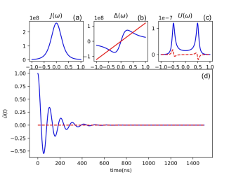
Figure 2: (a) The q-Gaussian spectral density $J(\omega)$ with respect to the frequency $\omega$ in the unit of $\Omega_{R}$ (after a central frequency shift $\omega-\omega_{s}\rightarrow\omega$, with $\omega_{s}=\omega_{c}$), which is also the imaginary part of the self-energy. (b) The blue curve is the real part of the self-energy, the cross points with the red line is the solution of $\Delta(\omega){=}\omega$ at which $J(\omega)\neq 0$ so that there is no localized bound states. (c) The blue (real) and red (dot) curves are the real and imaginary parts of $U(\omega)$, respectively. (d) The inverse Laplace transformation of $U(\omega)$, i.e., the Green function $\tilde{u}(t,t_{0})$. Here we plot the real and imaginary parts [the blue (real) and the red (dot ) curves] of $\tilde{u}(t,t_{0})\equiv u(t,t_{0})e^{i\omega_{c}(t-t_{0})}$ with $t_{0}{=}0$.

Experimentally, the photon number is measured by detecting the transmission intensity of the cavity field. Our theory gives the solution to the cavity photon number, i.e., Eq. (13b) which is divided into four terms. The first term represents the dissipation of the initial photons in the cavity. The second term is the photons injected into the cavity through the driving field. The third term shows the photon quantum fluctuations induced by the spin ensemble and the environment. The last term indicates the interference between the initial cavity photons and injected photons. In the experiment Putz14 , the cavity system is initially set in the vacuum. Hence, the first and the last terms are equal to zero in Eq.(13b) so that it is simply reduced to

$$\langle n(t)\rangle =|y(t,t_{0})|^{2}+v(t,t),$$ (27)

where $y(t,t_{0})$ and $v(t,t)$ are given by Eq. (12) which is determined by the solution of the Green function Eq. (26).

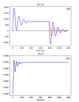
Figure 3: (a) The blue line is the evolution of the driving-field-induced cavity field $\tilde{y}(t,t_{0}){=}y(t,t_{0})\mathrm{e}^{i\omega_{c}(t{-}t_{0})}$, in which the dampings are caused by the spin ensemble for the q-Gaussian spectral density, and a rectangular driving field is applied with the resonant frequency $\omega_{p}=\omega_{c}=\omega_{s}$. The red-dashed line is given by Eq. (29) for the time duration $t\geq t_{\text{off}}$. (b) The photon fluctuation $v(t,t)$ of Eq. (12b) induced by spin ensemble at temperature 25 mK, which is negligible in comparison with the driving-field-induced cavity field $|y(t,t_{0})|^{2}$.

The solutions of $y(t,t_{0})$ and $v(t,t)$ are plotted in Fig. 3 in which $\tilde{y}(t,t_{0}){=}y(t,t_{0})\mathrm{e}^{i\omega_{c}(t{-}t_{0})}$. It shows that the driving-field-induced cavity field undergoes two damping processes. The first damping takes place when photons are injected into the cavity through a rectangular driving field. The cavity photons are raised up to the maximum very quickly. Meantime they are dissipated into the spin ensemble which is described Eq. (12a) through the Green function $u(t,t_{0})$, the corresponding oscillation decay is similarly shown in Fig. 2(d). The decay lasts a certain time $t_{s}$ ($t_{s}<600$ ns for the parameters given in Putz14 ), and the cavity photons gradually reach a saturation, i.e., $y(t_{s},t_{0})\simeq y(t_{\text{off}})=\langle a^{\dagger}(t_{\text{off}})\rangle$ after $t_{s}\simeq 600$ ns. Also note that the oscillating decay is a manifestation of the non-Markovian cavity decoherence induced by the inhomogeneous broadening of the spin ensemble spectrum, as we will see more later.

After the driving field is turned off at the time $t_{\text{off}}$, the cavity field undergoes the second damping, as shown by the blue solid line in Fig. 3(a). This result is directly obtained from the solution of $y(t_{\text{off}}+\tau,t_{0})$ which can be reduced to

$$\tilde{y}(t_{\text{off}}{+}\tau,t_{0}) =\tilde{y}(t_{\text{off}}){-}\tilde{y}(\tau,t_{0}),$$ (28)

which shows that the second damping process is off-phase with the first damping process. As a result, the time scale of the second damping in the observation of the cavity intensity is only a half of the decay time of the first damping, as shown in Fig. 4. On the other hand, the second damping process contains two parts, one is the re-started damping of the cavity field $y(t_{\text{off}})$ after the driving field is turned off, which is given by

$$\tilde{y}_{1}(t_{\text{off}}{+}\tau,t_{0}) =\tilde{y}(t_{\text{off}})\tilde{u}(\tau,t_{0}).$$ (29)

The result is shown by the red-dashed line in Fig. 3(a). The difference between the blue-solid line and the red-dashed line in Fig. 3(a) is the field retrieved from the spin ensemble. This part is the field retrieved back from the spin ensemble, as a demonstration of quantum memory in this hybrid systems Putz14 .

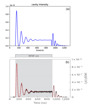
Figure 4: (a) The cavity intensity under a rectangular driving field calculated from our theory. (b) The cavity intensity measured (black curve) in experiment and the semiclassical description (red curve) given in Putz14 .

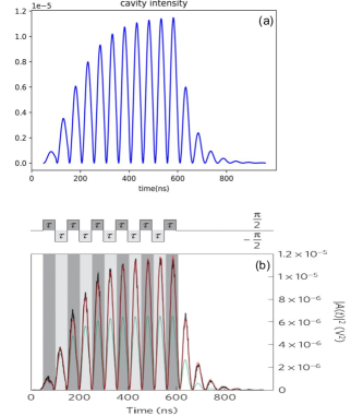
Figure 5: (a) The cavity intensity under a phase-shifting driving field calculated from our theory. (b) The cavity intensity measured (black curve) in experiment and the semiclassical description (red curve) presented in Putz14 .

With the above picture how the cavity field induced by the driving field is decohered (stored) into the spin ensemble and how it is retrieved back from the spin ensemble after the driving field is turned off, we present in Figs. 4(a) and 5(a) the cavity intensity of Eq. (27) with a rectangular driving field and a $\pi$ phase-shifting driving field, respectively, observed in the experiment Putz14 . Figures 4(a) and 5(a) show that our theoretical predictions are in good agreement with the experimental data presented in Figs. 4(b) and Fig. 5(b) of Ref. Putz14 . In fact, the authors of Ref. Putz14 used a semiclassical approach (the Volterra integral equation) to describe the cavity photon dynamics, and their results (see the red curves in Figs. 4(b) and Fig. 5(b)) also fitted the experimental data very well. This is because, when the injected photons through the driving field is very large ($\approx 10^{6}$) and the temperature is set to be very low ($\approx 25mK\sim\frac{1}{5}\hbar\omega_{c}$) in the experiment, the photon fluctuations given by $v(t,t)$ is indeed very very small, namely, $v(t,t)\ll|y(t,t_{0})|^{2}$, as shown in Fig. 3 [comparing the magnitude difference between Fig. 3(a) and Fig. 3(b)]. This gives the reason why the semiclassical approach used in Putz14 can fit very well with their experimental data.

On the other hand, the oscillation decays in Figs. 4 and 5 manifest the non-Markovian decoherence dynamics of the cavity field induced by the spin ensemble, here the cavity leakage is very small ($\kappa=2\pi\times 0.4$ MHz $\ll\Omega=2\pi\times 8.6$ MHz) in the experiment setup Putz14 . These oscillation decays can be characterized by the dissipation coefficient $\gamma(t,t_{0})$ in the exact master equation Eq. (II) and can be explicitly computed through Eq. (7a) which is again determined by the Green function $u(t,t_{0})$ of Eq. (26),

$$\gamma(t,t_{0})=-{\rm Re}[\dot{u}(t,t_{0})/u(t,t_{0})].$$ (30)

Some results are plotted in Fig. 6. Taking the same parameters used in experiment Putz14 , we find that when the coupling strength $\Omega/2\pi<2$ MHz, the Green function $u(t,t_{0})$ shows an exponential decay, see Fig. 6(a), which is the Markovian decoherence process. The corresponding decay rate is given by the asymptotic value of $\gamma(t,t_{0})$, see Fig. 6(c). The asymptotic value is $\gamma(t\rightarrow\infty,t_{0})\simeq 2\kappa+J_{s}(\omega_{s})$, as expected in the experiment observation in Putz14 .

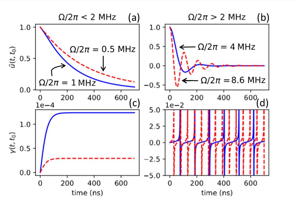
Figure 6: Decoherence dynamics of the cavity photons dissipating into the spin ensemble for different coupling strength $\Omega$ between the cavity and the spin ensemble, the same other parameters are taken as given in the experiment Putz14 . (a)-(b) The time evolution of the Green function $u(t,t_{0})$ for the coupling strength $\Omega/2\pi=0.5,1.0$ MHz and $4,8.6$ MHz, respectively; (c)-(d) The corresponding dissipation coefficient $\gamma(t,t_{0})$ determined by Eq. (30).

For the strong coupling regime (here $\Omega/2\pi>2$ MHz), the decoherence dynamics is very different. The Green function $u(t,t_{0})$ is no longer an exponential decay, it involves an oscillation decay for the cavity field as shown in Fig. 6(b). Such oscillations lead to the stronger oscillation of the dissipation coefficient $\gamma(t,t_{0})$ in time, as shown in Fig. 6(d). As it is well-known, such an oscillation shown in the dissipation coefficient between the positive and negative value is the strong effect of non-Markovian decoherence dynamics. In particular, the sudden change in the dissipation coefficient from a huge positive value to a huge negative value corresponds to the rapid forward and backward flows of photons (and information) between the cavity and the spin ensemble in a very short time. As the coupling becomes stronger and stronger, such rapid forward and backward flows of photons (or information) between the cavity and the spin ensemble get faster and faster. It is this unusual non-Markovian dynamics suppresses the cavity photon decoherence, as observed in this hybrid quantum system Putz14 . Also, such non-Markovian phenomena usually occurs in the symmetric spectral density with respect to the system energy state. This is the underlying mechanism how the decoherence induced by the inhomogeneous broadening is suppressed in the strong-coupling regime. This rapid forward and backward flows of photons between the cavity and the spin ensemble play a similar role of dynamical decoupling by a rapid, time-dependent control modulation to suppress decoherence DD1 ; DD2 even though the mechanisms of decoherence suppression are completely different. The former comes from the symmetric spectral density where the spectral density is the decoherence source, while the latter is generated from the external control pulses. Therefore, symmetricalized spectral densities may provide an alternative way to suppress decoherence for structured environments.

IV Decoherence suppression by hole-burning spectra

In another experiment of Putz et al. Putz17 , the spectral density of the spin ensemble is modified by the spectral hole burning technique. The spectral density after hole-burning frequencies at $\omega_{s}{\pm}\frac{\Omega_{R}}{2}$ is plotted in Fig. 1(a) [also see Fig. 7(a)]. In Fig. 7(b), the intersection points of the self-energy $\Delta(\omega)$ with the red line are located at frequencies $\omega_{s}{\pm}\frac{\Omega_{R}}{2}$, which could result in two localized modes Zhang2012 by the condition $\omega-\omega_{s}-\Delta(\omega)=0$ if the cavity leakage $\kappa$ can be ignored. It should be pointed out that the localize modes are the bound states of the cavity incorporating all possible modes of the spin ensemble. These localized modes are actually different from the dark states in quantum optics. Correspondingly, in Fig. 7(c), the two sharp peaks at $\omega_{s}{\pm}\frac{\Omega_{R}}{2}$ show the positions of the two localized modes, respectively. As a result, the Green function $u(t,t_{0})$ keeps oscillation in time, coming from these two localized modes, as shown in Fig. 7(d). In other words, the cavity field will not reach a steady state with the spin ensemble, as a dissipationless process induced by the localized modes due to the hole burning spectral density. This could change significantly the decoherence dynamics of the cavity field. Note that in principle, the peaks resulting from localized modes in Fig. 7(c) should be $\delta$-functions. However, due to the existence of a small cavity leakage ($\kappa\neq 0$), the peaks have a small finite width which results the cavity field in a slow decay in a very long time which is not shown in the Fig. 7(d).

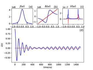
Figure 7: (a) The spectral density after the spectral hole burning. (b) The blue curve is the real part of the corresponding self-energy, the cross points with the red line are the solutions of $\Delta(\omega){=}\omega$, corresponds to the localized mode frequencies $\omega_{b}=\omega_{s}{\pm}\frac{\Omega_{R}}{2}$. (c) The real part (blue real line) and the imaginary part (red dot line) of the the spectrum of $u(t,t_{0})$. (d) The real part (blue real line) and the imaginary part (red dot line) of $\tilde{u}(t,t_{0})$ with $t_{0}{=}0$.

In the experiment Putz17 , the cavity transmission intensity is measured by applying a sinusoidal modulated pulse. Figure 8 shows a comparison of the cavity intensity with and without the spectral hole burning on the spin ensemble spectrum. Both the theoretical calculations and the experimental results show that, without the spectral hole burning, the cavity intensity has a linear decay in time after the driving field is turned off, see Fig. 8(a) and (b). While, with the spectral hole burning to the spin ensemble spectrum, the damping of the cavity intensity slows down significantly after the driving field is turned off, see Fig. 8(c) and 8(d). In other words, the coherence time is substantially improved. This is an effect of the dissipationless localized modes induced by the spectral hole burning of the spin ensemble.

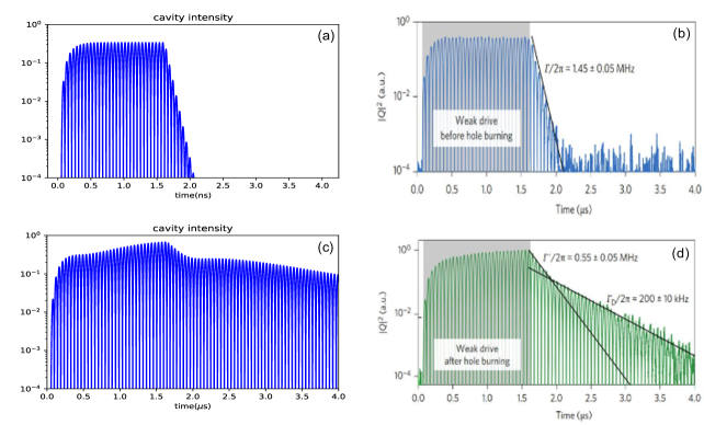
Figure 8: Cavity intensity for the q-Gaussian spectral density without (a-b) and with (c-d) the spectral hole burning, under a sinusoidal driving field, in which (a) and (c) the theoretical calculation from our theory; (b) and (d) are the experimental measurement by Putz et al. Putz17 .

Note that the theoretical and the experimental results shown in Fig. 8(c)-(d) do not fit each other very well. This is because the decoherence dynamics is very sensitive to the position and the shapes of the burning holes. In addition to the spectral hole burning at frequencies given in Putz17 , we also consider burning frequencies at different position to see how the decoherence dynamics of the cavity field sensitively depends on the shape of the spectral density. In Fig. 9(a), the spectrum is burnt at $\omega_{s}{=}\omega_{c}$. Theoretically, there may exist a localized mode at frequency $\omega_{s}$ if the cavity decay $\kappa$ can be negligible so that the decoherence can be suppressed. However, because the slope of $\Delta(\omega)$ at $\omega_{s}$ [see Fig. 9(a)] is so steep such that the amplitude of this localized mode is very small. In other words, the burning frequency almost has no effect on the cavity decoherence dynamics, as shown in the inset of Fig. 9(a). If the spectrum is burnt at $\omega_{s}{\pm}\frac{\Omega_{R}}{4}$ as shown in Fig. 9(b). Qualitatively, the decoherence dynamics is no much difference in comparing with the case without the hole burning, see in Fig. 2(d), although the decay is slow down a little bit. This shows that the burning frequencies must locate at the position of the intersection points with the red line in Fig. 9(b) so that the dissipationless localized modes can exist.

In summary, theoretically the suppression of cavity decoherence or the improvement of the transmission cavity field through the spectral hole-burning technique are resulted from the dissipationless localized modes between the system and the spin ensemble with gaped spectral density. In particular, these two localized modes are collective bound states (with many photons and spins) localized in energy domain Zhang2012 , which is quite different from usual dark states interpretation given in Putz17 . These states can be used to store (trap) information but are not easy to retrieve the information back. Therefore, it may not be useful for quantum memories but it can be used to serve as qubit states for quantum information processing, because these states can be made as decoherence-free states with specific design of spectral hole burning to the spin or atomic ensembles, even for heat ensembles.

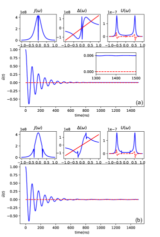
Figure 9: The same plot as Fig. 7 with different burning frequencies. (a) burning frequency at $\omega=\omega_{s}$. (b) A pair burning frequencies at $\omega=\omega_{s}{\pm}\frac{\Omega_{R}}{4}$.

V Characterizing Quantum memory with two-time correlation functions

As one sees, dynamical properties of the cavity system are fully determined by the Green function $u(t,\tau)$, from which one can find how the driving-field-induced cavity field $y(t,t_{0})$ changes inside the cavity through Eq. (12). It contains all the information on cavity decoherence induced by the spin ensemble through the spectral density $J_{s}(\omega)$. In this section, we show how the memory effect between the cavity and the spin ensemble can be explored specifically. To investigate the memory effect, we shall explore the two-time correlation functions, which measure the correlation of a past event with its future and therefore provide a physically observable definition of memory Ali2015 . Meantime, the two-time correlation function is now experimentally measurable in the real-time domain. In quantum optics, the familiar two-time correlation functions are the first-order and the second-order coherence functions, defined by

$$g^{(1)}(t,t+\tau) =\frac{\langle a^{\dagger}(t)a(t+\tau)\rangle}{\sqrt{\langle a^{\dagger}(t)a(t)\rangle\langle a^{\dagger}(t+\tau)a(t+\tau)\rangle}},$$ (31)

$$g^{(2)}(t,t+\tau) =\frac{\langle a^{\dagger}(t)a^{\dagger}(t+\tau)a(t+\tau)a(t)\rangle}{{\langle a^{\dagger}(t)a(t)\rangle}\langle a^{\dagger}(t+\tau)a(t+\tau)\rangle},$$ (32)

which can be calculated in terms of the functions $u(t,t_{0})$, $v(\tau,t)$ and $y(t,t_{0})$ in out theory. Explicitly,

$$\langle a^{\dagger}(t)a(t+\tau)\rangle= u^{*}(t,t_{0})u(t+\tau,t_{0})\langle a^{\dagger}(t_{0})a(t_{0})\rangle$$

$$+y^{*}(t,t_{0})y(t+\tau,t_{0})+v(t+\tau,t)$$

$$+u^{*}(t,t_{0})y(t+\tau,t_{0})\langle a^{\dagger}(t_{0})\rangle$$

$$+u(t+\tau,t_{0})y^{*}(t,t_{0})\langle a(t_{0})\rangle.$$ (33)

The second-order correlation function is more complicated although it can still be expressed in terms of the basic Green functions $u(t,t_{0})$, $v(\tau,t)$ and $y(t,t_{0})$.

Here we only present the result $\langle a^{\dagger}(t)a(t+\tau)\rangle$ to demonstrate the memory effect in this hybrid quantum system. Because the cavity is initially empty, the above solution is reduced to

$$\langle a^{\dagger}(t)a(t+\tau)\rangle=y^{*}(t,t_{0})y(t+\tau,t_{0})+v(t+\tau,t).$$ (34)

It shows that the coherence function is divided into two parts, the first part (the first term) is related to the coherence of the driving-field-induced cavity field at two different times, and the second term is associated with spin-ensemble-induced photon correlation. The cavity intensity presented in the previous two sections is the special case with the delay time $\tau=0$. In Fig. 4, it shows that the driving-field-induced cavity photons dissipate into the spin ensemble in a finite time scale, then the cavity field reaches a saturation (steady state). After turning off the driving field, the remained photons in the cavity continuously dissipate into the spin ensemble, mixed with some photons retrieved back from the spin ensemble. The question to ask is how these photons coherent with the photons previously injected into the cavity through the driving field.

Figure 10(a) shows the first-order coherence function $\langle a^{\dagger}(t)a(t+\tau)\rangle$ of the cavity field for a rectangular driving field with the same parameters used in Fig. 4. The result shows that the coherence between time $t$ and $t{+}\tau$ decays gradually before the driving field is turned off. However, once the driving field is turned off, the value of the first-order coherence drops to be a negative value. This negative correlation corresponds to an opposite $\pi$ phase coherence between the cavity fields at time $t$ and $t{+}\tau$, respectively. This is clearly shown by Eq. (28), and is manifested significantly in Fig. 10(a). Moreover, we have pointed out that this $\pi$-phase shift of the cavity field at a later time turns out a reduction of the damping oscillation period time by a half, which is also clearly seen in Fig. 10(a). On the other hand, Fig. 10(b) shows how the coherence function is changed by the spectral hole burning. The coherence behavior with the spectral hole burning is obviously lasted much longer, which indicates that the spectral hole burning can effectively suppress the decoherence and maintain the cavity field coherence for longer time.

Figure 10: First-order correlation (coherence) function $\langle\tilde{a}^{\dagger}(t)\tilde{a}(t+\tau)\rangle$ under the rectangular driving field (a) in the q-Gaussian spectral density and (b) with the spectral hole burning.

However, the coherence functions shown in Fig. 10 are acturaly dominated by the classical coherences or classical correlations because the cavity field contains a large number of photons (the order of $\sim 10^{6}$) which is in classical limit. To make the quantum coherence manifest, one should use a very weak driving field that maybe only contain one photon or less. The results are presented in Fig. 11.

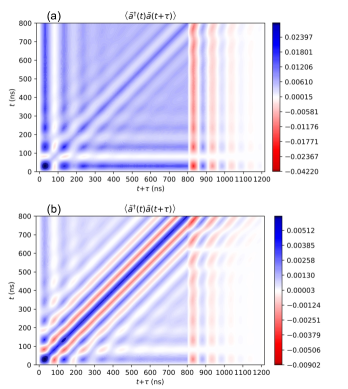
Figure 11: The same plot as Fig. 10 with a deduced driving field amplitude by an order of $10^{-4}$.

As one can see, after reduced down the driving field pulse by a order of $10^{-4}$, the two-time correlations are significantly changed. This change is mainly because the quantum noise correlation given by $v(t,t+\tau)$ becomes no longer negligible. The diagonal fringes in Fig. 11 are the manifestation of this quantum noise correlation.

To see more clear the quantum correlations, we plot the noise correlation alone by subtracting the classical part

$$\langle a^{\dagger}(t)a(t+\tau)\rangle-\langle a^{\dagger}(t)\rangle\langle a(t+\tau)\rangle=v(t+\tau,t)$$ (35)

The result is presented in Fig. 12. Actually the quantum noise correlation itself is independent from the driving field, it manifests the quantum memory effect between the cavity system and the spin ensemble, and is sensitive to the spectral structure of the spin ensemble. Figure 12(a) and (b) shows a clear difference of the quantum correlations between the q-Gaussian spectrum and the corresponding spectral hole burning. As one can see from Fig. 12(a) that without spectral hole burning, there is no obvious quantum correlation for the injected cavity field with cavity field after the driving field turned off. But with the spectral hole burning, the spin-ensemble-induced decoherence is suppressed and quantum memory can be maintained, which is displayed by the fringes in the right-bottom corner in Fig. 12(b). It shows a long time correlation or a long time quantum memory effect in this hybrid quantum systems, which should be interest to measure in further experiments.

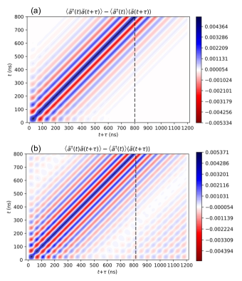
Figure 12: (a) First-order quantum correlation function in the q-Gaussian spectrum. (b) First-order quantum correlation function with the spectral hole burning.

VI Discussions and Outlook

In conclusion, we provide a master equation approach to study the decoherence dynamics of the hybrid quantum systems consisting of a microwave cavity coupled with an inhomogeneous broadening spin ensemble. The spin ensemble is made by negatively charged nitrogen-vacancy (NV) defects in diamond. Under the condition that less spins ($\sim 10^{6}$) are excited for a large spin ($\sim 10^{12}$) ensemble, the spin ensemble can be treated by a bosonic ensemble under the Holstein-Primakoff approximation, and from which we can derive the exact master equation for the cavity field. Our exact master equation describes the transient dynamics of the cavity system under the control of the external driving field in both the classical and the quantum regimes. The study of non-Markovian decoherence dynamics of the cavity coupled strongly to the spin ensemble is reduced to solve the Green functions $u(t,t_{0})$, $v(\tau,t)$ and $y(t,t_{0})$, i.e. Eqs. (12) and (26). These Green functions can be analytically solved and the results depict explicitly the detailed dissipation, quantum correlations and quantum memory effects in such hybrid quantum systems.

We apply the theory to the recent experiments by Putz et al. Putz14 ; Putz17 and interpret the corresponding experimental observation. Although the experimental observations have also been described with the semiclassical mean-field approach in terms of the Volterra integral equation in Putz14 ; Putz17 , or can be described by other approaches, such as the approaches presented in Refs. Kurucz11 ; Diniz11 ; Sandner11 , our results lead to a clearer physical picture of the decoherence. In particular, we find that the suppression of the decoherence induced by the inhomogeneous broadening of the spin ensemble in the strong-coupling regime is due to the rapid forward and backward photon flows between the cavity and the spin ensemble manifested in terms of the time-dependent dissipation coefficient in the master equation. The rapid forward and backward photon flows are also a typical non-Markovian decoherence effect. Such a rapid forward and backward photon flows become faster with the stronger coupling strength, manifested by the rapid oscillation of dissipation coefficient from the huge positive value to the huge negative value, see Fig. 6(d). It plays a similar role of dynamical decoupling by a rapid, time-dependent control modulation for decoherence suppression DD1 ; DD2 but it comes from the symmetric spectral density with respect to the cavity frequency rather than the external control pulses. This is the mechanism how the decoherence is suppressed in the strong-coupling regime in cavity QED. Moreover, the further suppression of decoherence through spectral hole burning Putz17 is due to the fact that the hole burning spectral density generates localized states which is dissipationless, as we pointed out early Zhang2012 .

We further explore the quantum memory in this hybrid quantum system through the two-time correlation functions. From a measurement perspective, the correlation between past events and their future is a measurable memory feature. We calculate the first-order coherence correlation function, and show how the cavity field correlated each other before and after the driving field turned off. In particular, we show how the quantum correlation or quantum memory can be manifested in the correlations function in the quantum regime with a low photonic intensity, which should be not difficult to be measured in experiments. Furthermore, based on our master equation, we can solve explicitly the reduce density matrix of the cavity field in this system, from which one can examine how the quantum states are stored in the spin ensemble and retrieved in a later time through quantum state tomography. This will remain in our further research.

- (1) S. Haroche and J.-M. Raimond, Exploring the Quantum: Atoms, Cavities, and Photons (Oxford University Press, New York, USA, 2006).
- (2) H. J. Carmichael, An Open Systems Approach to Quantum Optics, Lecture Notes in Physics m18 (Springer-Verlag, 1993).
- (3) H. J. Kimble and T. W. Lynn, Cavity QED with Strong Coupling - Toward the Deterministic Control of Quantum Dynamics, Coherence and Quantum Optics VIII Edited by Bigelow et aI. (Kluwer Academic/Plenum Publishers, 2003).
- (4) M. Brune, F. Schmidt-Kaler, A. Maali, J. Dreyer, E. Hagley, J. M. Raimond and S. Haroche, Quantum Rabi Oscillation: A Direct Test of Field Quantization in a Cavity, Phys. Rev. Lett. 76, 1800 (1996);
- (5) S. Brattke, B. T. H. Varcoe, and H. Walther, Generation of Photon Number States on Demand via Cavity Quantum Electrodynamics, Phys. Rev. Lett. 86, 3534 (2001).
- (6) R. J. Thompson, G. Rempe, and H. J. Kimble, Observation of normal-mode splitting for an atom in an optical cavity, Phys. Rev. Lett. 68, 1132 (1992).
- (7) C. J. Hood, M.S. Chapman, T. W. Lynn and H.J. Kimble, Real-Time Cavity QED with Single Atoms, Phys. Rev. Lett. 80, 4157 (1998).
- (8) J. McKeever, A. Boca, A.D. Boozer, R. Miller, J.R. Buck, A. Kuzmich and H.J. Kimble, Deterministic Generation of Single Photons from One Atom Trapped in a Cavity, Science 303, 1992 (2004)
- (9) A. Wallraff, D. I. Schuster, A. Blais, L. Frunzio, R.-S. Huang, J. Majer, S. Kumar, S. M. Girvin, and R. J. Schoelkopf, Strong coupling of a single photon to a superconducting qubit using circuit quantum electrodynamics, Nature 431, 162 (2004).
- (10) I. Chiorescu, P. Bertet, K. Semba, Y. Nakamura, C. J. P. M. Harmans, and J. E. Mooij, Coherent dynamics of a flux qubit coupled to a harmonic oscillator, Nature 431, 159 (2004).
- (11) Z. L. Xiang, S. Ashhab, J. Q. You, and F. Nori, Hybrid quantum circuits: superconducting circuits interacting with other quantum systems. Rev. Mod. Phys. 85, 623 (2013).
- (12) R. Amsüss, et. al., Cavity QED with Magnetically Coupled Collective Spin States, Phys. Rev. Lett. 107, 060502 (2011).
- (13) Y. Kubo, et al., Hybrid Quantum Circuit with a Superconducting Qubit Coupled to a Spin Ensemble Phys. Rev. Lett. 107, 220501 (2011).
- (14) S. Probst, et al., Anisotropic Rare-Earth Spin Ensemble Strongly Coupled to a Superconducting Resonator, Phys. Rev. Lett. 110, 157001 (2013).
- (15) H. Huebl, et al., High Cooperativity in Coupled Microwave Resonator Ferrimagnetic Insulator Hybrids, Phys. Rev. Lett. 111, 127003 (2013).
- (16) Y. Tabuchi, et al., Hybridizing Ferromagnetic Magnons and Microwave Photons in the Quantum Limit, Phys. Rev. Lett. 113, 083603 (2014).
- (17) P. L. Stanwix, et al., Coherence of nitrogen-vacancy electronic spin ensembles in diamond, Phys. Rev. B 82, 201201(R) (2010).
- (18) Z. Kurucz, J. H. Wesenberg and K. Mlmer, Spectroscopic properties of inhomogeneously broadened spin ensembles in a cavity. Phys. Rev. A 83, 053852 (2011).
- (19) I. Diniz, et al. Strongly coupling a cavity to inhomogeneous ensembles of emitters: Potential for long-lived solid-state quantum memories. Phys. Rev. A 84, 063810 (2011).
- (20) K. Sandner, et al. Strong magnetic coupling of an inhomogeneous nitrogen-vacancy ensemble to a cavity. Phys. Rev. A 85, 053806 (2012).
- (21) S. Putz, et al., Protecting a spin ensemble against decoherence in the strong-coupling regime of cavity QED, Nat. Phys., 10, 720 (2014).
- (22) S. Putz, et al., Spectral hole burning and its application in microwave photonics, Nature Photonics, 11, 36 (2017).
- (23) D. O. Krimer, S. Putz, J. Majer and S. Rotter, Non-Markovian dynamics of a single-mode cavity strongly coupled to an inhomogeneously broadened spin ensemble, Phys. Rev. A 90, 043852 (2014).
- (24) D. O. Krimer, B. Hartl and S. Rotter, Hybrid quantum systems with collectively coupled spin states: suppression of decoherence through spectral hole burning. Phys. Rev. Lett. 115, 033601 (2015).
- (25) M. W. Y. Tu and W. M. Zhang, Non-Markovian decoherence theory for a double-dot charge qubit, Phys. Rev. B 78, 235311 (2008).
- (26) C. U. Lei, and W. M. Zhang, A quantum photonic dissipative transport theory, Ann. Phys. 327, 1408 (2012).
- (27) W. M. Zhang, P. Y. Lo, H. N. Xiong, M. W. Y. Tu, and F. Nori, General non-Markovian dynamics of open quantum systems, Phys. Rev. Lett. 109, 170402 (2012).
- (28) W. M. Zhang, Exact master equation and general non-Markovian dynamics in open quantum systems, Eur. Phys. J. Spec. Top. 227, 1849 (2019).
- (29) M. Tavis and F. W. Cummings, Exact solution for an N-molecule-radiation-field Hamiltonian, Phys. Rev. 170, 379 (1968).
- (30) H. Primakoff and T. Holstein, Many-body interactions in atomic and nuclear systems, Phys. Rev. 55, 1218 (1939).
- (31) M. M. Ali, P. Y. Lo, M. W. Y. Tu, and W. M. Zhang, Non-Markovianity measure using two-time correlation functions. Phys. Rev. A 92, 062306 (2015).
- (32) M. M. Ali, and W. M. Zhang, Nonequilibrium transient dynamics of photon statistics. Phys. Rev. A 95, 033830 (2017).
- (33) A. I. Lvovsky, B. C. Sanders, and W. Tittel. Optical quantum memory. Nat. Photonics, 3, 706, (2009).
- (34) C. U Lei and W. M. Zhang, Decoherence suppression of open quantum systems through a strong coupling to non-Markovian reservoirs, Phys. Rev. A 84, 052116 (2011).
- (35) P. Y. Yang, C. Y. Lin and W. M. Zhang, Transient current-current correlations and noise spectra, Phys. Rev. B 89, 115411 (2014).
- (36) P. Y. Lo, H. N. Xiong and W. M. Zhang, Breakdown of Bose-Einstein Distribution in Photonic Caystals, Sci. Rep. 5, 9423 (2015).
- (37) P. Y. Yang and W. M. Zhang, Master equation approach to transient quantum transport in nanostructures, Frontiers of Physics, 12, 127204 (2017).
- (38) P. Y. Yang and W. M. Zhang, Buildup of Fano resonances in time-domain in a double quantum dot Aharonov-Bohm interferometer, Phys. Rev. B 97, 054301 (2018).
- (39) H. L. Lai, Y. W. Huang, P. Y. Yang, and W. M. Zhang, Exact master equation and non-Markovian decoherence dynamics of Majorana zero modes under gate-induced charge fluctuations, Phys. Rev. B 97, 054508 (2018).
- (40) H. T. Tan, and W. M. Zhang, Non-Markovian dynamics of an open quantum system with initial system-reservoir correlations: A nanocavity coupled to a coupled-resonator optical waveguide, Phys. Rev. A 83, 032102 (2011).
- (41) P. Y. Yang, C. Y. Lin, and W. M. Zhang, Master equation approach to transient quantum transport in nanostructures incorporating initial correlations, Phys. Rev. B 92, 165403 (2015).
- (42) L. Viola, E. Knill, ands S. Lloyd, S. Dynamical Decoupling of Open Quantum Systems, Phys. Rev. Lett. 82 2417 (1999).
- (43) W. Yang, Z. Y. Wang, and R. B. Liu, Preserving qubit coherence by dynamical decoupling, Frontiers of Physics, 6, 2 (2010).