A didactic approach to the Machine Learning application to weather forecast

Abstract

We propose a didactic approach to use the Machine Learning protocol in order to perform weather forecast. This study is motivated by the possibility to apply this method to predict weather conditions in proximity of the Etna and Stromboli volcanic areas, located in Sicily (south Italy). Here the complex orography may significantly influence the weather conditions due to Stau and Foehn effects, with possible impact on the air traffic of the nearby Catania and Reggio Calabria airports. We first introduce a simple thermodynamic approach, suited to provide information on temperature and pressure when the Stau and Foehn effect takes place. In order to gain information to the rainfall accumulation, the Machine Learning approach is presented: according to this protocol, the model is able to “learn” from a set of input data which are the meteorological conditions (in our case dry, light rain, moderate rain and heavy rain) associated to the rainfall, measured in mm. We observe that, since in the input dataset provided by the Salina weather station the dry condition was the most common, the algorithm is very accurate in predicting it. Further improvements can be obtained by increasing the number of considered weather stations and time interval.

I Introduction

The Earth’s atmosphere is a part of a very complex system, known as Earth System Sciences. In addition to the atmosphere, it also includes the hydrosphere (the water envelope formed by seas, rivers, lakes and underground waters), the cryosphere (the part of the Earth’s surface that is covered from the ice), the biosphere (the set of areas of the Earth in which the conditions necessary for animal and plant life exist) and the lithosphere (the outermost part of the Earth, formed by two layers, the crust and the mantle) Wallace:77 . Generally, the atmosphere is divided into different layers on the basis of the vertical profile of the temperature (temperature gradient) or on the basis of particular physical or chemical phenomena characterizing it. The temperature gradient allows one to identify the various atmospheric layers on the basis of the different characteristics between them Orlanki:75 . It is possible to identify two macro layers of the atmosphere: in the heterosphere (altitude $\geq$ 100 km) the average molecular free path is greater than one meter. Under these conditions the concentration of the heavier elements decreases with the altitude, compared to the lighter ones and there is no dependence with the vertical profile of the temperature. In the omosphere (altitude $\leq$ 100 km) the concentration of the main constituents tends to be uniform and independent of altitude due to the turbulent mixing; there is dependence on the vertical temperature profile. In the omosphere it is possible to identify the following layers of the atmosphere: troposphere, stratosphere, and mesosphere. A pictorial view of troposphere and stratosphere is reported in Fig. 1, where the separation between them (tropopause) is also visible. Among the different atmospheric layers, the troposphere plays a fundamental role since it contains the eighty percent of the total mass of the atmosphere; it also contains almost all the water vapor and, therefore, is the location where meteorological phenomena develop Fletcher:62 .

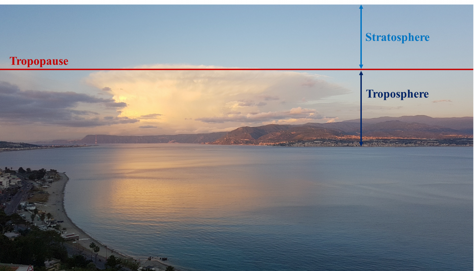
Figure 1: Visual representation of the troposphere and stratosphere, along with the separation between them, called tropopause.

Usually, in the troposphere there is a constant decrease in temperature with the altitude: this is due both to the possibility for an atmospheric layer to expand adiabatically (less pressure and therefore cooling) and, expecially, to the fact that the main source of heat is provided by the soil. The decreasing trend of the temperature with the altitude in the troposphere is the basis of the condensation phenomenon of the water vapor due to the orographic forcing. In this context, when the motion of mass of air is hampered by the presence of an orographic obstacle, the mass it is forced to rise. In this case, as the altitude increases, the temperature decreases. This cooling causes the condensation of water vapor thus favoring the genesis of extensive cloud systems with precipitation on the windward side (Stau effect). Then, when the air mass reaches the leeward slope, it starts a downward motion, with a corresponding increse of the pressure and therefore heating by adiabatic compression (Foehn effect). These effects occur especially in areas with a complex orography such as that which characterizes the Sicily region. The most important examples in this context are constituted by Etna and Stromboli volcanic areas. In particular, with its height of 3300 meters and its proximity to the Peloritani and Nebrodi mountains, Etna can favor the cooling and subsequent heating of the air masses, thus acting as a trigger for the genesis of even extreme weather events. Indeed, in the Ionian area of Sicily, it is not unusual that rainfall accumulations on the ground close to 300 mm in 2-3 hours occur MTCaccamo:17 . In principle, a proper knowledge of the nucleation processes Restuccia:18 and of cloud microphysics Castorina:19 could be significantly helpful, but, due to the complex weather conditions, this is not a straightforward task. In this context, the need to develop novel approaches suited to predict or reproduce such weather events clearly emerges.
The aim of the present work is twofold: from the one hand, we plan to provide a didactic explanation of the complex weather phenomena usually happening in region characterized by a complex orography, such as the Etna and Stromboli volcanic areas. From the other hand, we also develop a novel strategy to perform weather forecast avoiding the implementation of complex mathematical models and making use of the Machine Learning approach. The Machine Learning technique uses data to identify useful information without needing to know any mathematical formulas or specific codes, since the algorithm generates its own logic, based on the data entered in input and output Alpaydin:20 . One of these algorithms is called classification: it can insert data into different groups based on common characteristics that it is able to identify them independently. Learning can be supervised or unsupervised: the first one must know the previous answers to the problem (also called training data) and is able to work backwards to understand the logic between input and output. Instead, the unsupervised has no known answers to the problem used for training and the training set is not labeled as in the supervised case. The Machine Learning protocol has been recently implemented to predict weather forecast uncertainty Scher:18 , measure raindrops Denby:01 , perform drought forecasting for ungauged areas Rhee:17 and apply nowcasting methods based on real‐time reanalysis data Han:17 .
In this work, we illustrate how to apply the Machine Learning techniques to the weather forecasting. The input signals are get by sensors providing data related to the most important physical quantities (for instance temperature, pressure, rainfall, etc.) taken from fixed stations located in Sicily. Data concerning the output signals are related to the weather forecast of the days at issue, taking into account that the weather condition is affected by the input data. The work is organized as follows: in the next section a thermodynamic approach to describe the Stau and Foehn effects is presented; the Machine Learning technique is described in Section 3 and the results are presented in Section 4. Conclusions follow in the last section.

II Weather conditions and complex orography: the cases of the Stau and Foehn effects

A forced lifting occurs when a moving mass of air is forced to rise in front of an orographic obstacle (forced orographic ancestry). Lifting speeds are in the range of [0.5 - 1] m/s, with a decrease in temperature in the unit of time greater than that observed in large baric centers. The cooling, in general, causes the condensation of water vapor with extensive cloud formations and rainfall on the windward side. If the air is initially unsaturated, its upward movement takes place along a dry adiabatic, with a cooling rate of 1 ^∘C every 100 meters, up to the level where this cooling does not produce condensation: indeed the heat released by the condensation attenuates the cooling of the rising air. The lifting continues according to the saturated adiabatic with a thermal gradient that depends on the initial values of temperature, specific humidity and ascent rate. A realistic value for this thermal gradient is approximately 0.5 - 0.6 ^∘C per 100 meters. The upward movement of the air on the windward side of a mountain range (for example the Etna and Stromboli volcanic areas), with the formation of clouds and rainfall is called the Stau effect. In this phase, the abundant rainfall dry the rising air mass. When the latter crosses the leeward slope, in its downward motion, it undergoes an adiabatic compression with a corresponding heating of 1 ^∘C every 100 meters. This heat gain, not used to re-evaporate the clouds formed in the ascent phase (now dry air masses) is absorbed entirely by the air mass, which therefore reaches ground in a warmest and driest condition than it was originally. This is know as Foehn effect. The adiabatic expansions and compressions are well known examples of thermodynamic processes and have been recently investigated also by means of the Rüchardt’s experiment MTCaccamo:19 and the frequency analysis procedure Castorina:18 . The Stau and Foehn effects can be thermodynamically described by making use of the first thermodynamic law, which can be written as:

$$\Delta U=Q-L\,,$$ (1)

where $\Delta U$ indicates the variation of the internal energy of a thermodynamic system and $Q$ and $L$ are the amount of heat adsorbed by the system and the work performed by the system on the surrounding environment. Since, in the case of the Stau and Foehn effects, the thermodynamic process takes place without exchanging heat with the environment (i.e. adiabatically), $Q=0$. Therefore, Eq. 1 amounts to:

$$\Delta U=-L\,.$$ (2)

Since both the effects can be studied through an adiabatic process, for the sake of simplicity here we discuss in detail the Foehn effect only. According to the Foehn effect, the altitude decreases during the process, and hence the pressure increases, this leading to an adiabatic compression. Assuming the approximation of the ideal gases, the infinitesimal variation of internal energy can be written as follows:

$$dU=nC_{V}dT\,,$$ (3)

where $n$ is the number of moles, $C_{V}$ the specific heat at constant volume and $dT$ the infinitesimal variation of the temperature. Since the work performed by the systems corresponds to its pressure multiplied by the volume change, combining Eqs. 2 and  3 we obtain:

$$pdV=dL=-dU=-nC_{V}dT\,.$$ (4)

The equation of perfect gases can be written in a differential form as:

$$d(pV)=d(nRT)\rightarrow pdV+Vdp=nRdT\,,$$ (5)

where $R$ is the universal gas constant. By using Eq. 4, Eq. 5 may be rewritten as:

$$Vdp=nRdT+nC_{V}dT\,.$$ (6)

Eq. 6 my be expressed in terms of the specific heat at constant pressure, $C_{P}$, which is defined as:

$$C_{P}=R+C_{V}\,.$$ (7)

Therefore, Eq. 6 becomes:

$$Vdp=nC_{P}dT\,.$$ (8)

By dividing Eq. 8 by Eq. 4 we obtain:

$$\frac{Vdp}{pdV}=-\frac{nC_{P}dT}{nC_{V}dT}=-\frac{C_{P}}{C_{V}}=-\gamma\,,$$ (9)

where $\gamma$ is defined as the ratio $C_{P}/C_{V}$. By rearranging Eq. 9, a useful relation between pressure and volume can be found:

$$\frac{dp}{p}=-\gamma\frac{dV}{V}\,,$$ (10)

which, after integration, provides the result:

$${\rm ln}\frac{p_{f}}{p_{i}}=-\gamma{\rm ln}\frac{V_{f}}{V_{i}}\,,$$ (11)

where the indexes $f$ and $i$ label the final and initial state, respectively. Eq. 11 can be rearranged in turn as:

$$p_{i}V_{i}^{\gamma}=p_{f}V_{f}^{\gamma}\,,$$ (12)

which is known as Poisson equation; the latter, finally, leads to the expression:

$$pV^{\gamma}=constant\,,$$ (13)

which provides the relation between pressure and volume in the course of the adiabatic transformation which takes places during the Foehn effect. However, Eq. 13 does not provide any information on the temperature. The latter can be obtained by combining Eq. 12 with the equation of the perfect gases:

$$pV=nRT\,.$$ (14)

From Eq. 12 and Eq. 14 we obtain:

$$p_{i}\bigg{[}\frac{nRT_{i}}{p_{i}}\bigg{]}^{\gamma}=p_{f}\bigg{[}\frac{nRT_{f}}{p_{f}}\bigg{]}^{\gamma}\,,$$ (15)

which can be rewritten as:

$$p_{i}^{1-\gamma}T_{i}^{\gamma}=p_{f}^{1-\gamma}T_{f}^{\gamma}\,.$$ (16)

A proper rearrangement of Eq. 16 provides:

$$T_{i}p_{i}^{\frac{1-\gamma}{\gamma}}=T_{f}p_{f}^{\frac{1-\gamma}{\gamma}}\,.$$ (17)

For the sake of simplicity, we define a new constant $\alpha\equiv\frac{1-\gamma}{\gamma}$; therefore, Eq. 17 becomes:

$$T_{i}p_{i}^{\alpha}=T_{f}p_{f}^{\alpha}\,.$$ (18)

By taking the logarithm of both the members of Eq. 18 we obtain:

$${\rm ln}(T_{i})+\alpha{\rm ln}(p_{i})={\rm ln}(T_{f})+\alpha{\rm ln}(p_{f})\,,$$ (19)

which can be rearranged into:

$${\rm ln}\bigg{(}\frac{T_{i}}{T_{f}}\bigg{)}=\alpha{\rm ln}\bigg{(}\frac{p_{f}}{p_{i}}\bigg{)}\,.$$ (20)

Now we can rewrite $\alpha$ as follows:

$$\alpha\equiv\frac{1-\gamma}{\gamma}=\frac{1-C_{P}/C_{V}}{C_{P}/C_{V}}=\frac{C_{V}-C_{P}}{C_{P}}\,.$$ (21)

Since $C_{V}=C_{P}-R$, Eq. 21 finally becomes:

$$\alpha=\frac{C_{P}-R-C_{P}}{C_{P}}=-\frac{R}{C_{P}}\,.$$ (22)

Combining Eq. 22 with Eq. 20 we obtain:

$${\rm ln}\bigg{(}\frac{T_{i}}{T_{f}}\bigg{)}=-\frac{R}{C_{P}}{\rm ln}\bigg{(}\frac{p_{f}}{p_{i}}\bigg{)}\,,$$ (23)

which, after rearranging the second member, finally turns into:

$${\rm ln}\bigg{(}\frac{T_{i}}{T_{f}}\bigg{)}=\frac{R}{C_{P}}{\rm ln}\bigg{(}\frac{p_{i}}{p_{f}}\bigg{)}\,.$$ (24)

Eq. 24 provides a clear relationship between the values of temperature and pressure at the beginning and at the end of the adiabatic transformation and therefore is particularly useful in order to gain knowledge on these thermodynamic variables during the process. In particular, upon setting $p_{i}=1000$ hPa, corresponding to the atmospheric pressure at the sea level, it is possible to introduce the concept of potential temperature $\Phi$:

$$\Phi=T_{f}\frac{p_{0}}{p_{f}}{\rm exp}\bigg{[}\frac{R}{C_{P}}\bigg{]}\,.$$ (25)

The potential temperature indicates the final temperature reached by an atmospheric layer during an adiabatic expansion or compression from a given initial state till to the sea-level pressure. An important consequence of the definition of potential temperature is that it does not depend on the altitude $z$, i.e.

$$\frac{d\Phi}{dz}=0\rightarrow\Phi=constant\,.$$ (26)

As a consequence, its value does not change during the whole adiabatic process. A surface defined by Eq. 26 is known as isentropic surface and an atmospheric layer which lies on such a surface will remain on it in the course of the adiabatic transformation. Further details on the way to obtain the potential temperature, along with its numerous applications, can be found in Ref. Molders:14 .
It emerges that, under adiabatic conditions, many information on the weather conditions can be gained by using simple thermodynamic relationships. On the other hand, this approach can not provide information on other physical quantities, such as rainfall accumulations or wind speed, that are of great importance for a proper determination of the weather conditions. For such an aim, in parallel to the thermodynamic approach, we propose a novel methodology for the weather forecast, based on the Machine Learning protocol, which is discussed of the next section.

III The Machine Learning approach

The Machine Learning protocol is schematically depicted in Fig. 2.

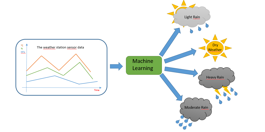
Figure 2: Illustration of the four different weather conditions investigated in this work by using the Machine Learning approach.

As can be seen from the graphical representation, the approach learns directly from the data. Specifically, we provide the input and output data to the algorithm and the software “will have to learn” how to solve the problem; this step is defined as a real training. The model so obtained can be used to define the meteorological activity which will be defined in four different conditions:
1. Dry;
2. Light rain;
3. Moderate rain;
4. Heavy rain.
A block illustration of the model workflow is provided in Fig. 3: a proper definition of the model is not a simple task, since data can come from many different sources, including sensors, images or database. Another important aspect concerns the data preprocessing, which requires specific algorithms for a specific application domain. For instance, if the input data are constituted by images, we must use algorithms that extract the features, whereas if they are constituted by historical series, statistical algorithms are needed. A proper choice of the most accurate algorithm among the large amount of possible protocols can require long time; usually, the best model is that one which guarantees a good balance between speed, accuracy and complexity. The last step of the procedure requires to iteratively repeat the workflow that led us to identify the best model.

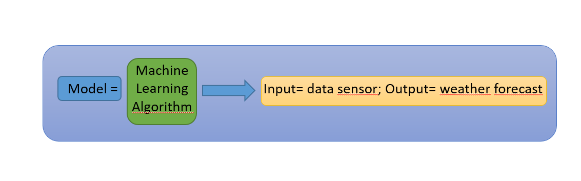
Figure 3: Schematic representation of the Machine Learning workflow.

We can divide the workflow into two steps, as shown in Fig. 4. The first step is the training, where the data coming from the weather stations are first processed by using statistical methods, and then a classifier is applied on the processed data, in order to build the model. The latter is then obtained through several iteration cycles. During the second step we use the trained model to perform the prediction, and therefore a new dataset is provided for testing the neural network.

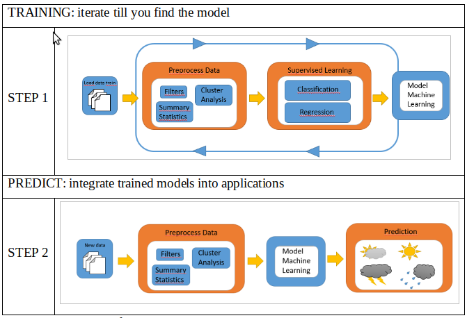
Figure 4: Illustration of the two steps of training and prediction.

In this context it is worth to point out the importance to have as much data as possible. In the present work, the input data for the training phase are physical quantities determining the weather conditions and are listed below:
1. Wind speed [m/s] and direction [^∘];
2. Atmospheric pressure [hPA];
3. Maximum and minimum humidity [%];
4. Maximum and minimum temperature [^∘C];
5. Rainfall [mm].
These data have been recorded by the weather station located on the island of Salina and have been provided by SIAS (Sicilian Agrometeorological Information Service), and collected with an hourly frequency for the days considered.

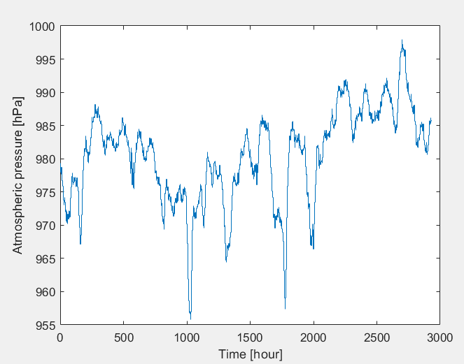
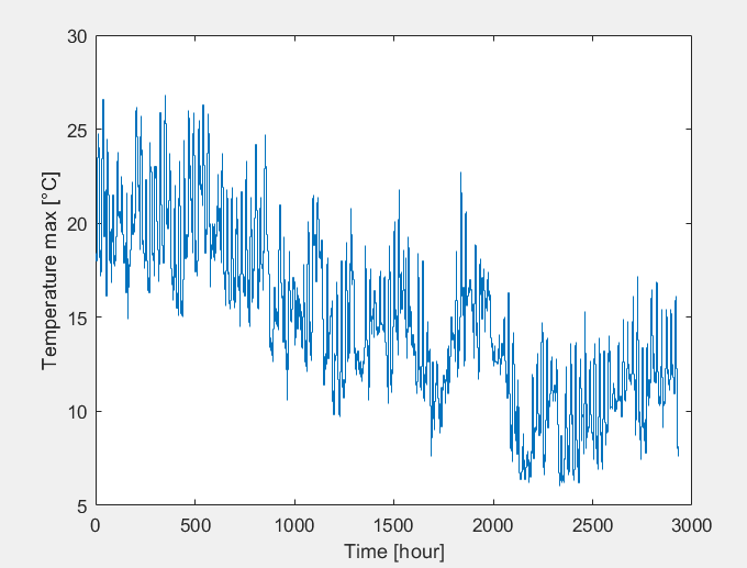
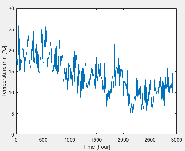
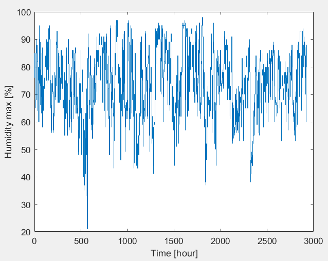
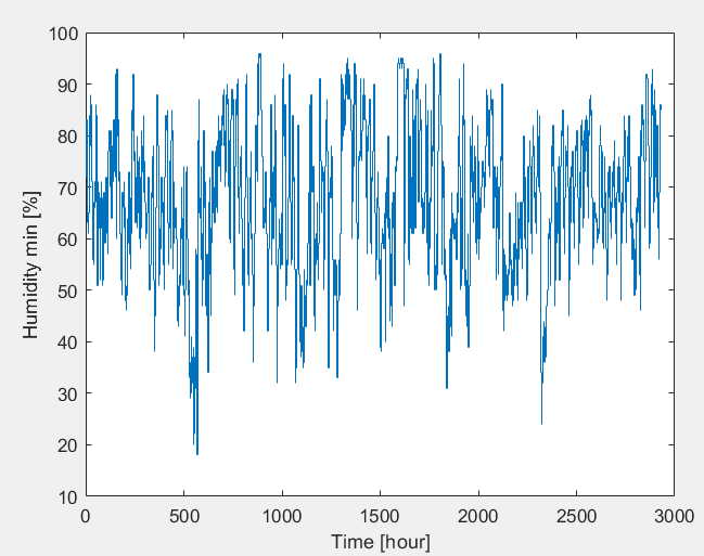
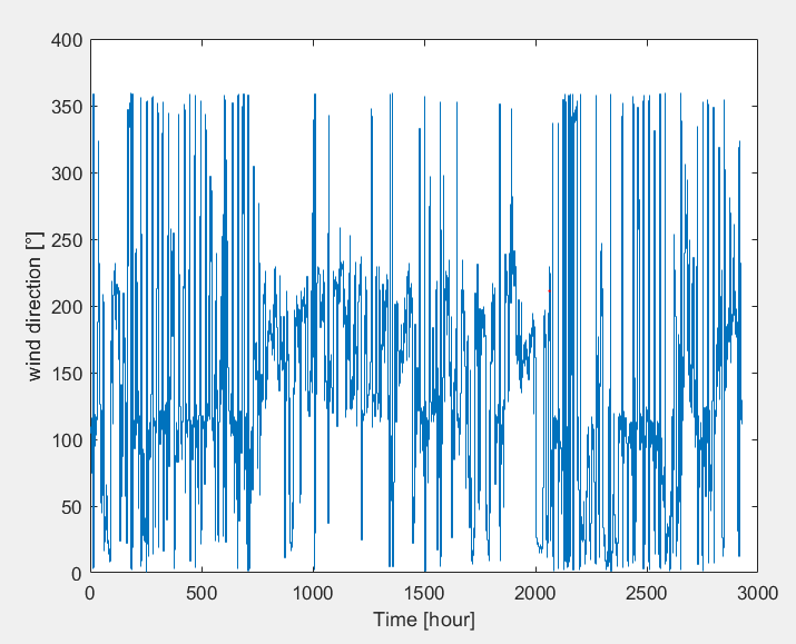
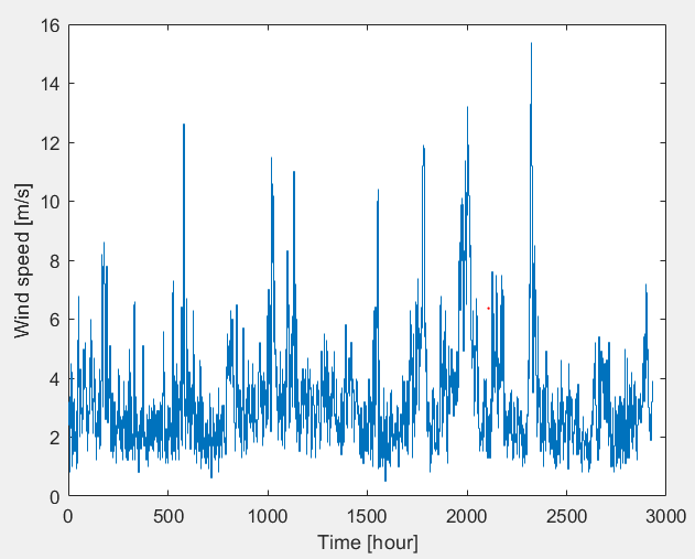
Figure 5: Input data for the model training obtained from the Salina weather station.

Such data, plotted in Fig. 5, cover a time interval going from 10/01/2019 to 01/31/2020, collecting 2929 total measurements. The data implemented for the functional test of the Machine Learning algorithm are 1945 measurements made from 02/01/2020 to 04/21/2020. The Machine Learning approach adopted in the present work is defined as a classification method and the algorithm is called supervised; in the training phase, this type of model needs to know the answers, i.e. the output of a given event. The input data of the system are provided by the Salina weather station which records every hour of every day certain quantities such as temperature, humidity, pressure, speed and wind direction. The output data that provide the wanted weather condition on a certain hour of a certain day are given by the measured rainfall. In particular, we have set the following matches Giuliacci:03 :
1. Dry occurs when there is no rainfall;
2. Low rain occurs when rainfall is less than 2 mm/h;
3. Moderate rain occurs when rainfall is between 2 and 6 mm/h;
4. Heavy rain occurs when rainfall is greater than 6 mm/h.
By using these information, the input data are classified through the weather condition, so that the system can be trained to recognize which physical quantities come into play in the determination of a rainfall. For such an aim, an Excel file was organized with all the data imported from the Salina weather station. The workflow for organizing such data is reported in Fig. 6.

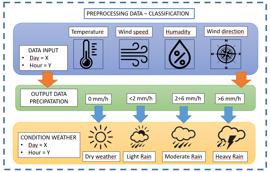
Figure 6: Schematic representation of the data organization according to the Machine Learning protocol.

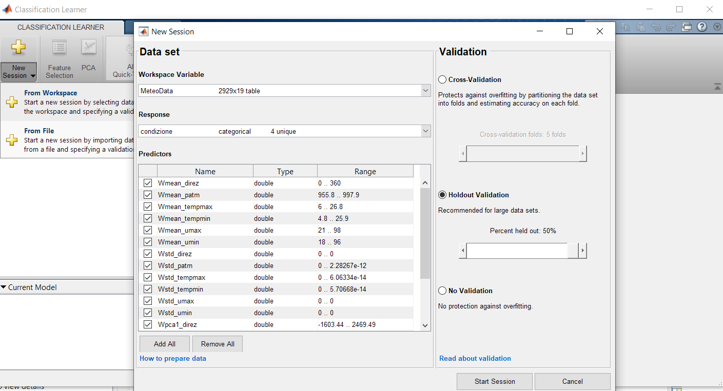
Figure 7: Schematic description of the Classification Learner K-Nearest Neighbours (KNN).

After the data organization, the next step concerns the data preprocessing: for such an aim, the Matlab software has been implemented. In particular, after importing the data into the workspace, it is necessary to manipulate these data in order to make it easily usable by our Machine Learning algorithms, through extraction of features; the extraction has been performed by means of the statistical laws, and in particular by using average value functions, standard deviation functions and functions of the analysis of the main components. After performing this transformation, we need to create a table that includes all the data. The next step is the opening of the Classification Learner which is a Matlab function whose task is to import the table containing the data (see Fig. 7). In this phase it is possible to choose the method for the data validation among two possible mechanisms: the first one is called cross-validation and is used in case of few available data, with the software trying to make more efficient use of such data. The second case is known as holdout validation and allows one to select some data for the validation and the remaining amount of data for the training phase; in this study, we have applied both the methods with the same frequency. When the data are read by the classifier, it is possible to choose the algorithm among those selectable to start the training phase. In Fig. 8 it is possible to note the percentages that refer to the prediction accuracy of the algorithm defined as K-Nearest Neighbours (KNN) Liu:16 .

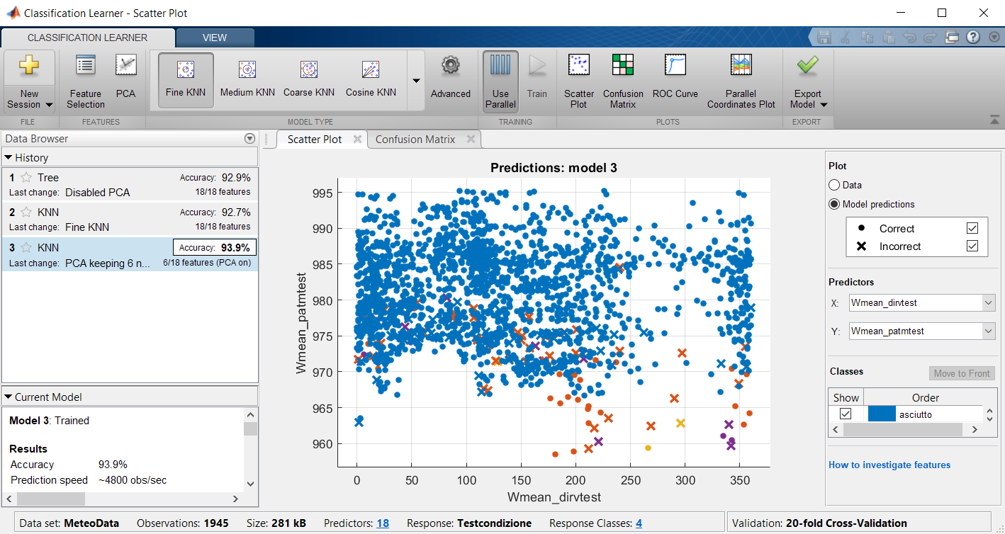
Figure 8: Prediction accuracy of the Classification Learner KNN.

IV The Machine Learning predictions

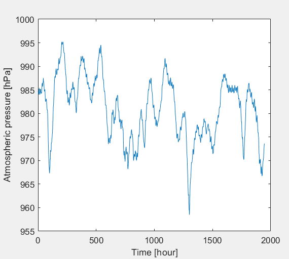
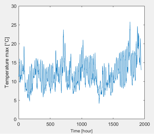
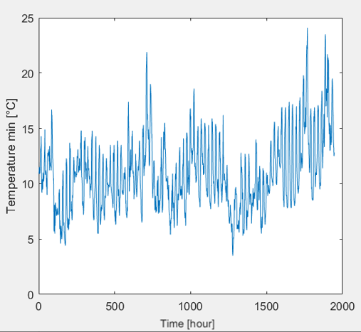
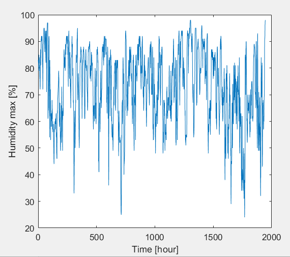
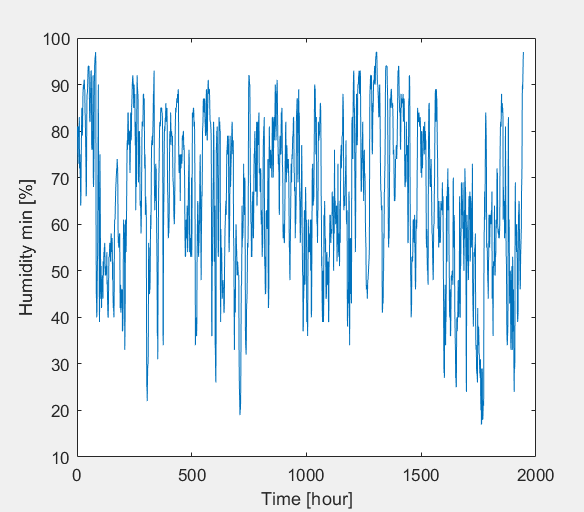
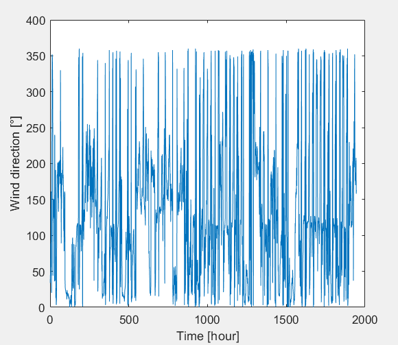
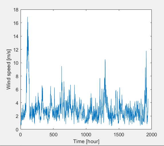
Figure 9: Input data for the model test.

The last step of the training phase is the export of the model; subsequently, another data set was taken, for the testing phase of the Machine Learning algorithm, with a different time span from that of the training. The data were treated in the same way as the training data: in particular, they are processed by using Excel, through the association of the physical quantities with the meteorological condition detected. Then, the data are imported on Matlab and finally statistical models for feature extraction (average, standard deviation and analysis of the main components) are applied. The input data for the model test are collectively shown in Fig. 9: in close analogy with the training data, also in this case the hourly values of atmospheric pressure, maximum and minimum temperature and humidity, and wind speed and direction are reported over the whole temporal interval. The testing phase consists on the compilation of an algorithm for plotting the results. This algorithm is written on Matlab, and it is suited to make a comparison between the real conditions measured by the weather stations and the prediction that the trained model carries out. To evaluate the quality of an algorithm, it is possible to use tools making the Classification Learner available. A largely adopted example of these tools is constituted by the confusion matrix reported in Fig. 10. The rows of this matrix indicate the model predictions, while columns refer to the data measured by the weather stations. Each matrix element show the correspondence (expressed in percentage) between predicted and observed data Choi:16 . The accuracy of the algorithm can be deduced by looking at the main diagonal, which shows (in green) the correct predictions. All other (wrong) predictions, corresponding to the other matrix elements, are reported in red. In particular, in Fig. 10 it can be seen that the dry condition is very well predicted, with an accuracy of 98%: this clearly depends on the amount of data chosen for testing the program, where the dry days are the majority. This problem could be solved by extending the data acquisition time to a larger period and increasing the number of weather stations examined. It is worth noting that, due to the approximation to unity, the sum of all the elements on a row does not exactly match the 100%. In addition, we also note that the element corresponding to the fourth row and third column is white, since this particular combination was never observed by the algorithm.

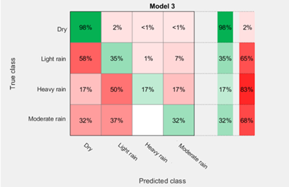
Figure 10: Machine Learning results represented through the confusion matrix.

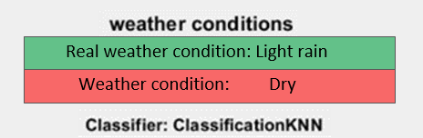
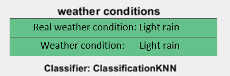
Figure 11: Accuracy of the Machine Learning predictions of the different weather conditions.

The prediction performances can be summarized in a more intuitive way in Fig. 11: here, when the correspondence between predicted and observed data is good, we can identify two green rectangles, which show real and the predicted weather conditions, respectively. According to the confusion matrix, the dry condition is almost always guessed. In the other panels of Fig. 11 it is possible to note the existence of incorrect predictions, indicated by the red rectangles. Finally, in the last panel we have reported two green rectangles also for the case of weak rain, since, after the dry case, this is the best reprented condition, even though the accuracy is only of 35%.

V Conclusions

In the present work we have presented a didactic approach suited to describe the Machine Learning application to the general problem of weather forecast. In particular, we have been focused on the predictions of weather conditions on geographic areas characterized by a complex orography, such the case of Sicily. A well known example is provided by the Etna and Stromboli volcanoes, whose presence significantly influences the weather conditions, due to Stau and Foehn effects, with possible impact on the air traffic of the nearby Catania and Reggio Calabria airports. We have shown that it is possible to use a simple thermodynamic approach to calculate the final temperature of a mass of air undergoing an adiabatic expansion or compression, such in the case of Stau and Foehn effects, but no information are provided on the rainfall accumulation. For such an aim we have proposed a Machine Learning approach which, while being only at its initial formulation, is able to provide indication on the weather conditions after a proper training phase with data input provided by the Salina weather station. Specifically, in the case at issue we have shown that the algorithm shows a great accuracy in predicting a dry condition, since the data provided by the analyzed weather station registered mostly this particular condition. The Machine Learing protocol described in the present work can be easily improved, for instance by enriching it with further input data and enlarging the time span considered.

References

- (1) J. M. Wallace and P. V. Hobbs, Atmospheric science: An introductory survey. Academic Press (New York), 1977.
- (2) I. Orlanski, “A rational subdivision of scales for atmospheric process,” Bull. Am Meteorol. Soc., vol. 56, no. 5, 1975.
- (3) N. H. Fletcher, The Physics of Rainclouds. Cambridge University Press, 1962.
- (4) M. T. Caccamo, G. Castorina, F. Colombo, V. Insinga, E. Maiorana, and S. Magazù, “Weather forecast performances for complex orographic areas: Impact of different grid resolutions and of geographic data on heavy rainfall event simulations in sicily,” Atmos. Res., vol. 198, pp. 22–33, 2017.
- (5) G. Castorina, M. T. Caccamo, S. Magazù, and L. Restuccia, “Multiscale mathematical and physical model for the study of nucleation processes in meteorology,” A.A.P.P., vol. 96, p. A6, 2018.
- (6) G. Castorina, M. T. Caccamo, and S. Magazù, “Study of convective motions and analysis of the impact of physical parametrization on the wrf-arw forecast model,” A.A.P.P., vol. 97, p. A19, 2019.
- (7) E. Alpaydin, Introduction to Machine Learning. MIT Press, 4th ed., 2020.
- (8) S. Scher and G. Messori, “Predicting weather forecast uncertainty with machine learning,” Q. J. R. Meteorol. Soc., vol. 144, pp. 2830–2841, 2018.
- (9) B. Denby et al., “Combining signal processing and machine learning techniques for real time measurement of raindrops,” IEEE Trans. Instrum. Meas., vol. 50, pp. 1717–1724, 2001.
- (10) J. Rhee and J. Im, “Meteorological drought forecasting for ungauged areas based on machine learning: Using long-range climate forecast and remote sensing data,” Agric. For. Meteorol, vol. 237-238, pp. 105–122, 2017.
- (11) L. Han, J. Sun, W. Zhang, Y. Xiu, H. Feng, and Y. Lin, “A machine learning nowcasting method based on real‐time reanalysis data,” IEEE Trans. Instrum. Meas., vol. 122, pp. 4038–4051, 2017.
- (12) M. T. Caccamo, G. Castorina, F. Catalano, and S. Magazù, “Rüchardt’s experiment treated by fourier transform,” Eur. J. Phys., vol. 40, p. 025703, 2019.
- (13) G. Castorina, M. T. Caccamo, and S. Magazù, “A new approach to the adiabatic piston problem through the arduino board and innovative frequency analysis procedures,” in New Trends in Physics Education Research (S. Magazù, ed.), pp. 133–156, Nova science publishers, 2018.
- (14) N. Mölders and G. Kramm, Lectures in Meteorology. Springer, 2014.
- (15) A. G. M. Giuliacci and P. Corazzone, Manuale di meteorologia. Alpha test, 2003.
- (16) Z. Liu and Z. Zhang, “Solar forecasting by k-nearest neighbors method with weather classification and physical model,” 2016 North American Power Symposium (NAPS), pp. 1–6, 2016.
- (17) S. Choi, Y. J. Kim, S. Briceno, and D. Mavris, “Prediction of weather-induced airline delays based on machine learning algorithms,” 2016 IEEE/AIAA 35th Digital Avionics Systems Conference (DASC), pp. 1–6, 2016.