Learning Hamiltonian Monte Carlo in R

Abstract

Hamiltonian Monte Carlo (HMC) is a powerful tool for Bayesian computation. In comparison with the traditional Metropolis-Hastings algorithm, HMC offers greater computational efficiency, especially in higher dimensional or more complex modeling situations. To most statisticians, however, the idea of HMC comes from a less familiar origin, one that is based on the theory of classical mechanics. Its implementation, either through Stan or one of its derivative programs, can appear opaque to beginners. A lack of understanding of the inner working of HMC, in our opinion, has hindered its application to a broader range of statistical problems. In this article, we review the basic concepts of HMC in a language that is more familiar to statisticians, and we describe an HMC implementation in R, one of the most frequently used statistical software environments. We also present hmclearn, an R package for learning HMC. This package contains a general-purpose HMC function for data analysis. We illustrate the use of this package in common statistical models. In doing so, we hope to promote this powerful computational tool for wider use. Example code for common statistical models is presented as supplementary material for online publication.

Keywords: Bayesian computation, Hamiltonian Monte Carlo, MCMC, Stan

1 Introduction

Hamiltonian Monte Carlo (HMC) is one of the newer Markov Chain Monte Carlo (MCMC) methods for Bayesian computation. An essential advantage of HMC over the traditional MCMC methods, such as the Metropolis-Hastings algorithm, is its greatly improved computational efficiency, especially in higher-dimensional and more complex models. But despite the method’s computational prowess and the existence of excellent introductions (Neal et al., 2011; Betancourt, 2017), practitioners still face daunting challenges in applying the method to their own applications. Difficulties mainly arise in three areas: (1) unfamiliarity with the theory behind the algorithm, (2) lack of understanding of how the existing software works, (3) inability to tune the HMC parameters. These difficulties have limited the use of HMC to those who understand the theory and have the programming skills to implement the algorithm. But it does not have to be so.

The emergence of modern Bayesian software such as Stan (Carpenter et al., 2017) has, to some extent, alleviated these difficulties. Stan is a powerful and versatile programming language that has a syntax similar to that of WinBUGS, but uses HMC instead of Gibbs sampling to generate posterior samples (Gelman et al., 2015). Stan translates its code to a lower-level language to maximize speed and efficiency. Importantly, it automates the tuning of HMC parameters and thus significantly reduces the burden of implementation. For R and Python users, packages have been created that allow Stan be called from those languages. For people who are familiar with WinBUGS and comfortable with programming in probabilistic terms, Stan is an ideal choice for HMC implementation. But for beginners who want to learn HMC, Stan can come across as a “black box”. Other high-performance software, such as PyMC and Edward (Salvatier et al., 2016; Tran et al., 2016), presents similar challenges. While scalability and efficiency are often the foremost considerations in software development, a good understanding of the methodology is more essential to learners, as it instills confidence in the practical use of new methods.

The objectives of the current paper are largely pedagogical, i.e., helping practitioners learn HMC and its algorithmic ingredients. Toward that end, we developed a general-purpose R function hmc for the fitting of common statistical models. We also present details of HMC parameter tuning for those who are interested in writing and implementing their own programs. Multiple examples are presented, with accompanying R code. We have assembled all of the learning material, including the necessary HMC functions, example code, and data in an R package, hmclearn, for convenience of the readers.

2 Markov Chain Monte Carlo: The Basics

MCMC is a broad class of computational tools for integral approximation and posterior sample generation. In Bayesian analysis, MCMC algorithms are primarily used to simulate samples for approximation of the posterior distribution.

In Bayesian analysis, estimation and inference of the parameter of interest are made based on the observed data $\mathcal{D}$ together with the a priori information that one has on the parameters of interest $\bm{\theta}=(\theta_{1},...,\theta_{k})^{T}\in\mathbb{R}^{k}$. The posterior distribution $f(\bm{\theta}|\mathcal{D})$ combines both the data and prior information in accordance to the Bayes formula, and is proportional to the product of the likelihood function $f(\mathcal{D}|\bm{\theta})$ and the prior density $f(\bm{\theta})$ (Carlin & Louis, 2008) ,

$$f(\bm{\theta}|\mathcal{D}) =\frac{f(\mathcal{D}|\bm{\theta})f(\bm{\theta})}{\int f(\mathcal{D}|\bm{\theta})f(\bm{\theta})d\bm{\theta}},$$

$$\propto f(\mathcal{D}|\bm{\theta})f(\bm{\theta}).$$

The integral in the denominator is usually difficult to evaluate. But since the denominator is constant with respect to $\bm{\theta}$, one could work with the unnormalized posterior $f(\mathcal{D}|\bm{\theta})f(\bm{\theta})$. In the absence of an explicit expression of the posterior, approximating it with simulated samples following $f(\bm{\theta}|\mathcal{D})$ becomes a desirable alternative.

2.1 Metropolis-Hastings

Metropolis algorithm is the first widely-used MCMC method for generating Markov Chain samples following $f(\bm{\theta}|\mathcal{D})$. The method originated from a physics application in the 1950’s (Metropolis et al., 1953), and was further extended nearly two decades later by Hastings (1970), thus giving rise to the name of Metropolis-Hastings (MH) algorithm. We begin with a brief description of MH, as HMC was built on a similar concept.

MH generates a sequence of values of $\bm{\theta}$ that form a Markov chain, whose values can be used to approximate a posterior density $f(\bm{\theta}|\mathcal{D})$. For brevity, we drop $\mathcal{D}$ from the expression and write the posterior simply as $f(\bm{\theta})$. Values in the Markov chain $\bm{\theta}^{(t)}$ are indexed by $t=0,1,..,N$, where $\bm{\theta}^{(0)}$ is a user or program-specified starting value.

MH defines a transition probability that assures the Markov chain is ergodic and satisfies detailed balance and reversibility (Chib & Greenberg, 1995). These technical conditions are put in place to ensure the chain samples from the full support of $\bm{\theta}$ without bias.

In MH, values of $\bm{\theta}^{(t)}$ in the chain are defined in part by a proposal density $q(\bm{\theta}^{\text{PROP}}|\bm{\theta}^{t-1})$, where $\bm{\theta}^{\text{PROP}}$ is a proposal for the next value in the chain. This proposal density is conditioned on the previous value $\bm{\theta}^{(t-1)}$. A variety of proposal functions can be used, with random walk proposals being the most common choice.

Algorithm 1 Metropolis-Hastings

1:procedure MH($\bm{\theta}^{(0)},f(\bm{\theta}),q(\bm{\theta}^{(1)}|\bm{\theta}^{(2)}),N$)

2:     Calculate $f(\bm{\theta}^{(0)})$

3:     for $t=1,...,N$ do

4:         $\bm{\theta}^{\text{PROP}}\leftarrow q(\bm{\theta}^{\text{PROP}}|\bm{\theta}^{(t-1)})$

5:         $u\leftarrow U(0,1)$

6:         $\alpha=\min\left(1,\frac{f(\bm{\theta}^{\text{PROP}})q(\bm{\theta}^{(t-1)}|\bm{\theta}^{\text{PROP}})}{f(\bm{\theta}^{(t-1)})q(\bm{\theta}^{\text{PROP}}|\bm{\theta}^{(t-1)})}\right)$

7:         If $\alpha<u$, then $\bm{\theta}^{(t)}\leftarrow\bm{\theta}^{\text{PROP}}$. Otherwise, $\bm{\theta}^{(t)}\leftarrow\bm{\theta}^{(t-1)}$

8:     end for

9:     return $\bm{\theta}^{(1)}...\bm{\theta}^{(N)}$

10:end procedure

In MH, a proposal is accepted with probability

$$\alpha=\min\left(1,\frac{f(\bm{\theta}^{\text{PROP}})q(\bm{\theta}^{(t-1)}|\bm{\theta}^{\text{PROP}})}{f(\bm{\theta}^{(t-1)})q(\bm{\theta}^{\text{PROP}}|\bm{\theta}^{(t-1)})}\right),$$ (1)

When $q$ is symmetric i.e., $q(\bm{\theta}^{(t-1)}|\bm{\theta}^{\text{PROP}})=q(\bm{\theta}^{\text{PROP}}|\bm{\theta}^{(t-1)})$, this simplifies to

$$\alpha=\min\left(1,\frac{f(\bm{\theta}^{\text{PROP}})}{f(\bm{\theta}^{(t-1)})}\right),$$

which is used in the original Metropolis algorithm.

The denominator in the posterior is constant with respect to $\bm{\theta}$. As such, the ratio of posterior densities at two different points $\bm{\theta}^{PROP}$ and $\bm{\theta}^{(t-1)}$ can be compared even when the denominator is unknown, with the denominators being cancelled out. Because a derivation of the full posterior distribution (numerator and denominator) is not necessary to implement MH (and HMC, as we will see), data analysts have considerable flexibility to select models of their liking.

The acceptance rate $\alpha$ in (1) is an important gauge of the efficiency of an MH algorithm. A careful examination of $\alpha$’s roles gives a more intuitive understanding of the algorithm:

1. When $f(\bm{\theta}^{PROP})\geq f(\bm{\theta}^{(t-1)})$, the proposal $f(\bm{\theta}^{PROP})$ represents a “more likely” value than the previous value $\bm{\theta}^{(t-1)}$, as quantified by the density functions. When this occurs, the proposal is always accepted (i.e. with probability 1).

2. When $f(\bm{\theta}^{PROP})<f(\bm{\theta}^{(t-1)})$, the proposal $\bm{\theta}^{PROP}$ has a lower density in comparison to the previous value, and we accept the proposal at random with probability $\alpha\in(0,1)$, which indicates the relative likelihood of observing $\bm{\theta}^{PROP}$ from $f$, as compared to $\bm{\theta}^{(t-1)}$. The larger the $\alpha$, the greater the chance of accepting $\bm{\theta}^{PROP}$. If the proposal is not accepted, the proposal will be discarded and the chain will remain in place $\bm{\theta}^{(t)}:=\bm{\theta}^{(t-1)}$, and we will start with a new proposal.

With such a scheme, the algorithm frequents regions of higher posterior density, while occasionally visiting the low density areas (e.g., tails in one-dimensional situations). Provided the algorithm satisfies the conditions for ergodicity (Tierney, 1994) and runs a sufficient number of iterations, the empirical distribution of the MCMC chain samples should approximate the true posterior density. The simulated values can therefore be used for estimation and inference based on the posterior distribution. See Carlin & Louis (2008) Chib & Greenberg (1995) Gelman et al. (2013) for additional details on MH.

2.2 Limitations of Metropolis-Hastings

The theoretical requirements for using MH are quite minimal, thus making it an attractive choice for Bayesian inference. Limitations of MH are primarily computational. With randomly generated proposals, it often takes a large number of iterations to get into areas of higher posterior density. Even efficient MH algorithms sometimes accept less than $25\%$ of the proposals (Roberts et al., 1997). In lower dimensional situations, increased computational power may compensate the lower efficiency to some extent. But in higher dimensional and more complex modeling situations, bigger and faster computers alone are rarely sufficient to overcome the challenge.

Gibbs sampling can be a viable and more efficient alternative to MH in some situations (Geman & Geman, 1987). In fact, several popular software platforms, such as WinBUGS and JAGS, use Gibbs to generate posterior samples (Lunn et al., 2000; Plummer et al., 2003). Gibbs’ requirement for explicitly expressed conditional posterior densities, however, has prevented it from being used in many practical situations. In addition to this restriction, Gibbs also has its own efficiency limitations (Robert, 2001). It is in this context that HMC emerges as a preferred alternative for Bayesian analysis.

3 Hamiltonian Monte Carlo

Hamiltonian Monte Carlo improves the efficiency of MH by employing a guided proposal generation scheme. More specifically, HMC uses the gradient of the log posterior to direct the Markov chain towards regions of higher posterior density, where most samples are taken. As a result, a well-tuned HMC chain will accept proposals at a much higher rate than the traditional MH algorithm (Roberts et al., 1997).

It is important to note that although the HMC algorithm frequently samples in regions of higher density, referred to as the typical set (Betancourt, 2017), it still samples the tail areas properly. While both MH and HMC produce ergodic Markov chains, the mathematics of HMC is substantially more complex than that of MH. In this paper, we provide a less technical introduction of the ideas behind HMC. More technical expositions can be found elsewhere (Neal et al., 2011; Betancourt, 2017).

3.1 The idea

The methods one uses to generate proposals strongly influences the efficiency of MCMC. Suppose $f(\theta)$ is a one-dimensional posterior density function, and $-\log f(\theta)$ assumes the shape of an inverse bell-shaped curve as depicted by Figure 1. To generate $\theta$ in a region of high posterior density, one needs to sample $\theta$ in the region corresponding to the lower values of $-\log f(\theta)$; the region can be reached with the guidance of the gradient of $-\log f(\theta)$. In a sense, the approach is analogous to the movement of a hypothetical object on a frictionless curve, where the object traverses and lingers at the bottom of the valley while occasionally visiting the higher grounds on both sides. In classical mechanics, such movements are described by the Hamiltonian equations, where the exchanges of kinetic and potential energy dictate the object’s location at any given moment.

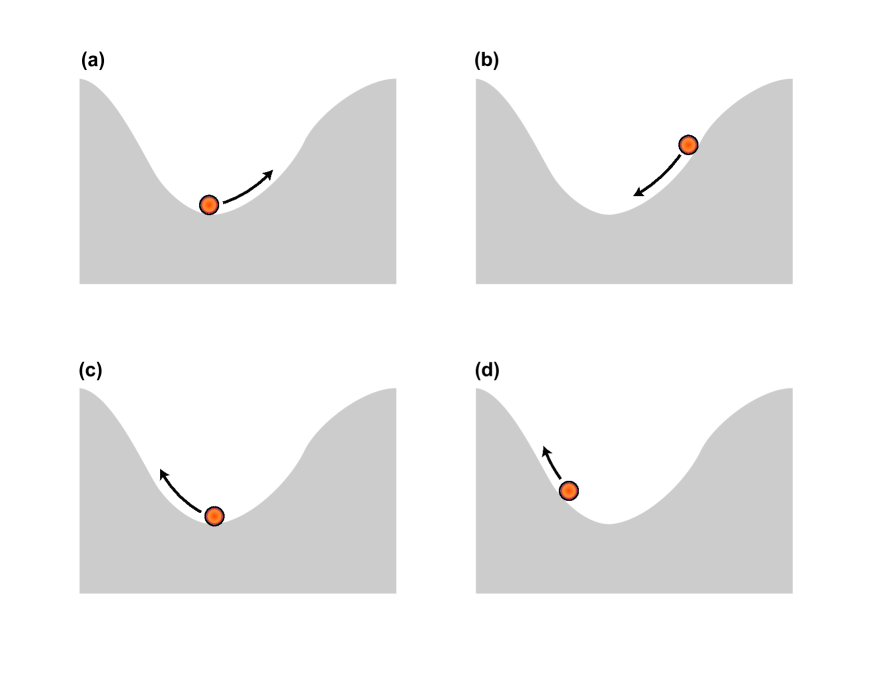
Figure 1: One-dimensional HMC example - movement of an object on a smooth, frictionless curve. (a) We apply a force with randomly generated direction and strength to the object. This object acquires a certain amount of kinetic energy, which makes it move in the direction of the applied force. The momentum, proportional to the object’s velocity, changes throughout the path of the curve. When the object moves up along the curve, the velocity of the object and its momentum decrease. Its kinetic energy converts to potential energy, while the total energy remains constant. (b) The object will stop at a point when all of its kinetic energy is converted to potential energy. The potential energy then makes the object move in the opposite direction, converting its potential energy back to kinetic energy. (c) At the lowest point of the curve, all of the energy is in the kinetic form (peak velocity/momentum), which pushes the object up to the left side of the curve. (d) As the object goes up on the curve, its kinetic energy again converts to potential energy, until all is in the form of potential energy. Then, the object would stop and then slide back as guided by its potential energy. Since the surface is frictionless, the total energy remains constant throughout these repeated movements.

In a Hamiltonian system, the horizontal and vertical positions are given by $(\theta,p)$. In MCMC, we are interested in $\theta$. The parameter $p$, which is often referred to as the momentum, is an auxiliary quantity that we use to simulate $\theta$ under the Hamiltonian equations.

3.2 The Hamiltonian Equations

We introduce HMC in a generic MCMC setting, where $\bm{\theta}$ follows the posterior density $f(\bm{\theta})$ of interest, and the momentum $\mathbb{p}$ is generated from a parametric distribution. The momentum matches the dimensionality of $\bm{\theta}$ as a vector of length $k$.

We write the Hamiltonian function as $H(\bm{\theta},\mathbb{p})$, which consists of potential energy $U(\bm{\theta})$ and kinetic energy $K(\mathbb{p})$: $H(\bm{\theta},\mathbb{p})=U(\bm{\theta})+K(\mathbb{p})$, where $\mathbb{p}$ and $\bm{\theta}\in\mathbb{R}^{k}$.

In statistical applications of MCMC, we are primarily interested in generating $\bm{\theta}$ from a given distribution $f(\bm{\theta})$. To do so, we let $U(\bm{\theta}):=-\log f(\bm{\theta})$. Such a designation would ensure $\bm{\theta}$ generated from the Hamiltonian function follows the desired distribution. For momentum, we typically assume $\mathbb{p}\sim N_{k}(0,\mathbb{M})$, where $\mathbb{M}$ is a user-specified covariance matrix.

Under this formulation, we have

$$H(\bm{\theta},\mathbb{p})=-\log f(\bm{\theta})+\frac{1}{2}\mathbb{p}^{T}\mathbb{M}^{-1}\mathbb{p}.$$ (2)

Over time, HMC travels on trajectories that are governed by the following first-order differential equations, known as the Hamiltonian equations

$$\begin{split}\frac{d\mathbb{p}}{dt}&=-\frac{\partial H(\bm{\theta},\mathbb{p})}{\partial\bm{\theta}}=-\frac{\partial U(\bm{\theta})}{\partial\bm{\theta}}=\nabla_{\bm{\theta}}\log f(\bm{\theta}),\\ \frac{d\bm{\theta}}{dt}&=\frac{\partial H(\bm{\theta},\mathbb{p})}{\partial\mathbb{p}}=\frac{\partial K(\mathbb{p})}{\partial\mathbb{p}}=\mathbb{M}^{-1}\mathbb{p},\end{split}$$ (3)

where $\nabla_{\bm{\theta}}\log f(\bm{\theta})$ is the gradient of the log posterior density. A solution to the Hamiltonian equations is a function that defines the path of $(\bm{\theta},\mathbb{p})$ from which specific values of $\bm{\theta}$ could be sampled. Within an MCMC iteration, we sample a value $\bm{\theta}$ from this path. The randomness of the MCMC samples comes from the momentum $\mathbb{p}\sim N_{k}(0,\mathbb{M})$ and the specific $\bm{\theta}$ value we choose.

3.3 Solving the Hamiltonian Differential Equations

Solving the Hamiltonian equations, therefore, becomes a critical step in HMC simulation. A standard approach for solving differential equations is Euler’s method, which produces a discrete function that approximates the solution at each time t. Values of $(\bm{\theta},\mathbb{p})$ that satisfy the Hamiltonian equations would be legitimate values for the HMC. But as Neal et al. (2011) have noted, errors tend to accumulate in Euler’s method, especially after a larger number of steps. In HMC, one often has to take a larger number of steps to ensure the new proposal is sufficiently far from the location of the previous sample.

The leapfrog method is a good alternative to the standard Euler’s method for approximating the solutions to Hamiltonian equations (Ruth, 1983). The leapfrog algorithm modifies Euler’s method by using a discrete step size $\epsilon$ individually for $\mathbb{p}$ and $\bm{\theta}$, with a full step $\epsilon$ in $\bm{\theta}$ sandwiched between two half-steps $\epsilon/2$ for $\mathbb{p}$,

$$\begin{split}\mathbb{p}(t+\epsilon/2)&=\mathbb{p}(t)+(\epsilon/2)\nabla_{\bm{\theta}}\log f(\bm{\theta}(t)),\\ \bm{\theta}(t+\epsilon)&=\bm{\theta}(t)+\epsilon\mathbb{M}^{-1}\mathbb{p}(t+\epsilon/2),\\ \mathbb{p}(t+\epsilon)&=\mathbb{p}(t+\epsilon/2)+(\epsilon/2)\nabla_{\bm{\theta}}\log f(\bm{\theta}(t+\epsilon)).\end{split}$$ (4)

For HMC, multiple leapfrog steps are typically required to move a sufficient distance to the next proposal. Research has shown that discrete approximations remain accurate, even after many steps. The stability of the leapfrog algorithm is due to the leapfrog’s symplectic property. (Channell & Scovel, 1990; Betancourt, 2017). Symplecticity ensures that the volume of the support is preserved when mapping from one point to another, such as through one or more consecutive iterations of the leapfrog algorithm(Neal et al., 2011).

For a given momentum vector $\mathbb{p}$ within an HMC iteration, the path defined by the Hamiltonian equations is deterministic. Proposals generated from an exact solution of these equations, if achievable, would always be accepted. But since our solution from the leapfrog is an approximation, a Metropolis style accept/reject step is added to ensure the newly generated proposal does not deviate too far from the specified Hamiltonian $H(\bm{\theta},\mathbb{p})$. The acceptance rate of HMC proposals is therefore less than 100%, but generally higher than that of the Metropolis algorithm.

3.4 Hamiltonian Monte Carlo Algorithm

The flowchart in Figure 2 shows the key steps in HMC. Initial values for $\bm{\theta}$ and $\mathbb{p}$ are required to start the algorithm. With $\bm{\theta}^{(0)}$ and $\mathbb{p}^{(0)}$ specified, the leapfrog algorithm is used to find approximate solutions to the Hamiltonian equations. The leapfrog solutions define the path of $(\bm{\theta},\mathbb{p})$ over time within an iteration.

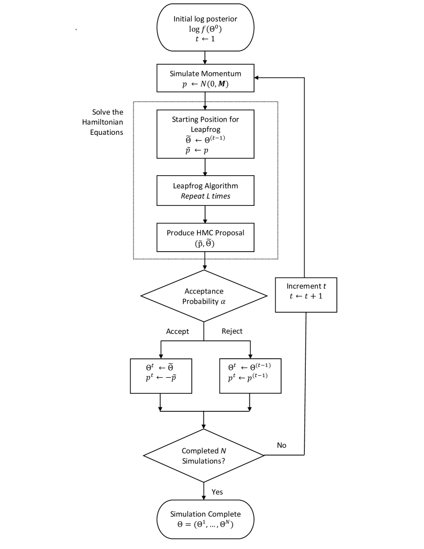
Figure 2: Main Steps of the Hamiltonian Monte Carlo Method

Typically, multiple steps, each of length $\epsilon$, are taken to generate an HMC proposal. Parameter $L$ represents the number of steps. While $L$ is often fixed to a positive integer value, some randomness can be introduced to ensure a valid exploration of the space of $(\bm{\theta},\mathbb{p})$. A generic HMC is given below in Algorithm 2.

Algorithm 2 Hamiltonian Monte Carlo

1:procedure HMC($\bm{\theta}^{(0)},\log f(\bm{\theta}),\mathbb{M},N,\epsilon,L$)

2:     Calculate $\log f(\bm{\theta}^{(0)})$

3:     for $t=1,...,N$ do

4:         ${\mathbb{p}}\leftarrow N(0,\mathbb{M})$

5:         $\bm{\theta}^{(t)}\leftarrow\bm{\theta}^{(t-1)},\tilde{\bm{\theta}}\leftarrow\bm{\theta}^{(t-1)},\tilde{\mathbb{p}}\leftarrow{\mathbb{p}}$

6:         for $i=1,...,L$ do

7:              $\tilde{\bm{\theta}},\tilde{\mathbb{p}}\leftarrow\text{Leapfrog}(\tilde{\bm{\theta}},\tilde{\mathbb{p}},\epsilon,\mathbb{M})$

8:         end for

9:         $\alpha\leftarrow\min{\left(1,\frac{\exp(\log{f(\tilde{\bm{\theta}}})-\frac{1}{2}{\mathbb{\tilde{p}}^{T}\mathbb{M}^{-1}{\mathbb{\tilde{p}})}}}{\exp(\log f(\tilde{\bm{\theta}}^{(t-1)})-\frac{1}{2}{\mathbb{p}^{T}}\mathbb{M}^{-1}\mathbb{p})}\right)}$

10:         With probability $\alpha$, $\bm{\theta}^{(t)}\leftarrow\tilde{\bm{\theta}}$ and $\mathbb{p}^{(t)}\leftarrow-\tilde{\mathbb{p}}$

11:     end for

12:     return $\bm{\theta}^{(1)},...,\bm{\theta}^{(N)}$

13:     function Leapfrog($\bm{\theta}^{*},\mathbb{p}^{*},\epsilon,\mathbb{M}$)

14:         $\tilde{\mathbb{p}}\leftarrow\mathbb{p}^{*}+(\epsilon/2)\nabla_{\bm{\theta}}\log f(\bm{\theta}^{*})$

15:         $\tilde{\bm{\theta}}\leftarrow\bm{\theta}^{*}+\epsilon\mathbb{M}^{-1}\tilde{\mathbb{p}}$

16:         $\tilde{\mathbb{p}}\leftarrow\tilde{\mathbb{p}}+(\epsilon/2)\nabla_{\bm{\theta}}\log f(\tilde{\bm{\theta}})$

17:         return $\tilde{\bm{\theta}},\tilde{\mathbb{p}}$

18:     end function

19:end procedure

As with other valid MCMC algorithms, HMC’s transition probability is designed to meet the theoretical requirements for detailed balance and reversibility. These conditions ensure that our HMC samples provide a valid representation of the posterior distribution. If we denote the transition probability from $\bm{\theta}^{(t)}$ to $\bm{\theta}^{(t+1)}$ as $T(\bm{\theta}^{(t)},\bm{\theta}^{(t+1)})$, then detailed balance requires that $f(\bm{\theta}^{(t)})T(\bm{\theta}^{(t)},\bm{\theta}^{(t+1)})=f(\bm{\theta}^{(t+1)})T(\bm{\theta}^{(t+1)},\bm{\theta}^{(t)})$. The HMC transition probability includes two components to ensure that detailed balance and reversibility hold true:

1. the accept/reject step, and

2. the negation of the momentum after the final leapfrog step.

The negated momentum illustrates the reversibility of HMC transitions, which can be demonstrated by stepping through the leapfrog from the proposed state to the original state. Tierney (1994) described the theoretical requirements for MCMC algorithms in general, while Betancourt (2017) provided a detailed exposition specific to HMC.

In Section 4, we describe a general-purpose function hmc in our proposed package. Within the package, the gradient functions for commonly used generalized linear mixed effect models under the default priors are provided. The hmc function can also take user-defined posterior density and gradient functions for non-standard statistical models. In situations where analytical derivation of gradient functions is infeasible, one could consider using numerical auto-differencing functions. Automated differencing libraries capable of calculating the gradient exactly such as the Stan math library (Carpenter et al., 2015), also called Autodiff, are appropriate for direct use in HMC applications.

3.5 HMC Tuning for Improved Efficiency

The efficiency of an HMC algorithm can be improved through parameter tuning and reparameterization. HMC tuning involves selection and adjustment of the various HMC parameters. Two parameters that need to be specified are the step size $\epsilon$ and the number of leapfrog steps $L$. Elements in the covariance matrix $\mathbb{M}$ may also be adjusted from the default identity matrix for efficiency improvement.

It is generally a good practice to set $\epsilon$ to a smaller value relative to the magnitude of the parameter of interest. A smaller $\epsilon$ results in closer approximations and thus higher acceptance rates. But a small $\epsilon$ must be coupled with a large $L$ to ensure the trajectory length $\epsilon L$ is large enough to move the simulated parameter to a distant point in the distribution. On the other hand, if $\epsilon L$ is too large the trajectory is likely to circle back, causing waste in simulation. To tune $\epsilon$ and $L$ is to find the right combinations of these values, which are usually chosen via monitoring the acceptance rate. Neal et al. (2011) suggested an optimal acceptance rate is approximately 65%. At the same time, it is often helpful to examine the trace plots of the MCMC samples for signs of autocorrelation. Slow-moving chains with stronger autocorrelation often indicate insufficient $\epsilon L$. While $\epsilon$ and $L$ can be tuned jointly, most analysts choose to select the step size first, then under a given step size, they fine-tune the number of steps per leapfrog $L$.

Additional adjustments may be made to the tuning parameters beyond these basic steps. For example, one could use different values of $\epsilon$ for each of the $k$ parameters in $\bm{\theta}$ to increase the sampling efficiency. The hmc function in hmclearn allows setting $\epsilon$ to a vector instead of a single number to give analysts the flexibility to use different step sizes for different parameters. The parameter for the number of steps $L$ must be a natural number. However, randomly chosen $L$ could be used to guard against periodicity of the Markov chain. The step size $\epsilon$ may also be randomized. In the hmc function, random $\epsilon$ and $L$ can be automatically applied via parameter setting. A useful algorithm known as the No U-Turn Sampler (NUTS) automatically selects $L$ for each sample; NUTS is a commonly used alternative to manual parameter tuning (Hoffman & Gelman, 2014).

The efficiency of sampling in the standard HMC algorithm can also be improved for multivariate models when the parameters have an orthogonal basis. One common method of ensuring an orthogonal basis involves applying QR decomposition (Voss, 2013) . In many statistical models, especially linear models, the design matrix helps to define the model itself and is central to the model fitting computation. In HMC, QR decomposition is often applied to the design matrix to create the orthogonal basis for sampling. Applying this transformation in practice can improve the computational efficiency of HMC for many models (Team, 2017). After the simulation is complete, the MCMC samples are transformed back to the original basis for inference.

4 A Package for Learning HMC

HMC presents considerable challenges to beginners attempting to learn the algorithm. First, the method can be difficult to comprehend because its idea originated from physics applications of the Hamiltonian equations. Second, it is often difficult to learn the inner working of HMC from programs such as Stan, because they are not designed as teaching tools. In fact, Stan specifies models in a probabilistic syntax and shields users from the actual HMC steps.

In this paper, we present an R package hmclearn to provide users with the software tools to learn the intricacies of the HMC, through explicit specification of log posterior and gradient functions, as well as parameter tuning. It is designed to give user a hands-on experience for implementing HMC analysis for a broad class of statistical models. Once users have understood and mastered the essential HMC steps, they could go on to write their own code for specific applications. To download hmclearn, go to https://cran.r-project.org/web/packages/hmclearn/index.html.

The core function in hmclearn is hmc, which is a general-purpose function for MCMC sample generation by using the HMC method. This function takes user-defined log posterior and gradient functions as inputs and produces MCMC samples. Here we do not ask for an explicit specification of prior $f(\bm{\theta})$ as an input function. Instead, we let users define their log posterior $\log f(\bm{\theta|}\bm{y})=\log f(\bm{y}|\bm{\theta})+\log f(\bm{\theta})$, which includes $f(\bm{\theta})$. Such a design reduces the number of required input functions, while preserving users’ flexibility in choosing different priors.

Other input parameters to hmc include the number of samples $N$, the step size $\epsilon$, the number of leapfrog steps $L$, and the Mass matrix $\mathbb{M}$. These are the essential elements to start an HMC simulation, but the user will typically need to adjust at least some of these parameters to tailor the simulation to their specific applications. Users are required to provide their own starting values for $\bm{\theta}$ when using the hmc function for their own applications. Examples of log posterior and gradient functions are provided in hmclearn for various generalized linear mixed effect models, which can be used as templates for less standard models.

Running multiple MCMC chains is often desirable to determine if each chain converges to the same distribution of $\bm{\theta}$. Since modern computers almost universally have multiple core processors, parallel processing can be an efficient way to run multiple chains at the same time. To that end, hmclearn includes parameters to enable parallel processing as well as multiple chains.

Finally, a variety of Bayesian graphical functions are provided based on the bayesplot package (Gabry & Mahr, 2016). Functionalities incorporated in hmclearn include trace plots, histograms, density plots, and credible interval plots. The integrated functions comprise the core diagnostic plotting functions typical for MCMC applications. Additional diagnostics can be programmed directly or called based on the output of the hmc function.

5 HMC in Statistical Models

5.1 A general process

In this section, we discuss the general steps of HMC implementation in statistical models. We describe the process through examples of generalized linear models. The major steps required to fit a statistical model are summarized in Figure 3. Following the steps illustrated in the diagram, one could generate HMC samples with user-specified posterior and gradient functions, by using the hmc function in the hmclearn package.

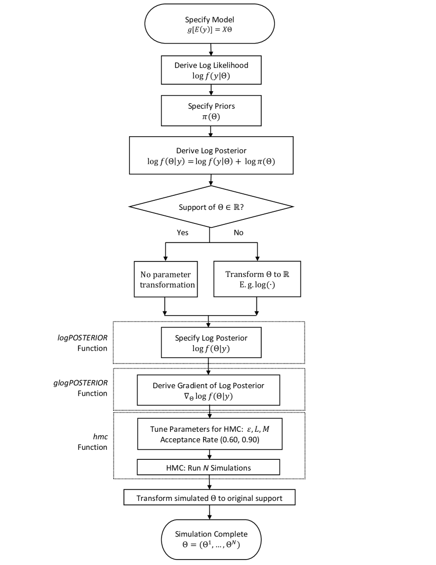
Figure 3: Major steps of HMC implementation

5.2 Examples

We present three examples to illustrate how to fit various linear models using HMC. Our notation for these examples reflects the programming of the sample log posterior and gradient functions in hmclearn. This programming uses matrix and vector multiplication instead of for loops, which can be computationally slow in R.

5.2.1 Example 1: Linear Regression

We consider a linear regression model $y_{i}=\mathbb{x}_{i}^{T}\bm{\beta}+\epsilon_{i}$, where $y_{i}$ is the response for the ith subject, $i=1,...,n$, and $\mathbb{y}=(y_{1},...,y_{n})^{T}$ is a vector of responses. The covariate values for the ith subject are $\mathbb{x}_{i}^{T}=(x_{i0},...,x_{iq})$, where $x_{i0}$ is frequently set to one as an intercept term for all subjects. We write the full design matrix as $\mathbb{X}=(\mathbb{x}_{1}^{T},...,\mathbb{x}_{n}^{T})^{T}\in\mathbb{R}^{n\times(q+1)}$. The regression coefficients for the $q$ covariates plus an intercept are written as $\bm{\beta}=(\beta_{0},...,\beta_{q})^{T}$. The error term for each subject is $\epsilon_{i}$. All error terms $\bm{\epsilon}=(\epsilon_{1},...,\epsilon_{n})^{T}$ are assumed to be independent and normally distributed with mean zero and constant variance $\sigma_{\epsilon}^{2}$.

The log likelihood for linear regression, omitting the constants, can be written as

$$\log f(\mathbb{y}|\bm{\beta},\sigma_{\epsilon}^{2})\propto-n\log\sigma_{\epsilon}-\frac{1}{2\sigma_{\epsilon}^{2}}(\mathbf{y}-\mathbf{X}\bm{\beta})^{T}(\mathbf{y}-\mathbf{X}\bm{\beta}).$$

We specify a multivariate normal prior for $\bm{\beta}$ with covariance matrix $\sigma_{\beta}^{2}\mathbb{I}$ where $\sigma_{\beta}^{2}$ is a hyperparameter set by the analyst, and an inverse gamma (IG) prior for $\sigma_{\epsilon}^{2}$. The IG prior has hyperparameters $a$ and $b$, which are also set by the analyst. We write

$$f(\bm{\beta}|\sigma_{\beta}^{2}) \propto\exp\left(-\frac{\bm{\beta}^{T}\bm{\beta}}{2\sigma_{\beta}^{2}}\right)\quad\textrm{ and}\quad f(\sigma_{\epsilon}^{2}|a,b) =\frac{b^{a}}{\Gamma{(a)}}(\sigma_{\epsilon}^{2})^{-a-1}\exp\left(-\frac{b}{\sigma_{\epsilon}^{2}}\right).$$

The support of $\sigma_{\epsilon}^{2}$ is $(0,\infty)$. We apply a logarithmic transformation to expand the support to $\mathbb{R}$. We have

$$\gamma =\log\sigma_{\epsilon}^{2},\quad\sigma_{\epsilon}^{2}=g^{-1}(\gamma)=e^{\gamma},$$

$$f(\gamma|a,b) =\frac{b^{a}}{\Gamma(a)}\exp\left(-a\gamma-\frac{b}{e^{\gamma}}\right),$$

$$\log f(\gamma|a,b) \propto-a\gamma-be^{-\gamma}.$$

The log posterior is proportional to the log likelihood plus the log prior,

$$\log f(\bm{\beta},\gamma|\mathbb{y},\mathbb{X},\sigma_{\beta}^{2},a,b) \propto-\left(\frac{n}{2}+a\right)\gamma-\frac{e^{-\gamma}}{2}(\mathbf{y}-\mathbf{X}\bm{\beta})^{T}(\mathbf{y}-\mathbf{X}\bm{\beta})-\frac{\bm{\beta}^{T}\bm{\beta}}{2\sigma_{\beta}^{2}}-be^{-\gamma}.$$

The parameters of interest are defined as $\bm{\theta}:=(\beta_{0},...,\beta_{q},\gamma)^{T}$, where $k=q+2$. To fit this model using hmc, the user must provide a function for the log posterior where the first function parameter is a vector for the parameters of interest $\bm{\theta}$. Additional function parameters can be included for the data and hyperparameters. An example log posterior function for this model and specification of priors is included in hmclearn.

The Hamiltonian function (2) is composed of the log posterior and the log density function of the momentum, where $\mathbb{p}\sim N_{k}(0,\mathbb{M})$. Writing the Hamiltonian function for our linear regression model is straightforward once the log posterior is developed,

$$H(\bm{\theta},\mathbb{p}) =H(\bm{\beta},\gamma,\mathbb{p})\propto\log f(\bm{\beta},\gamma|\mathbb{y},\mathbb{X},\sigma_{\beta}^{2},a,b)+\frac{1}{2}\mathbb{p}^{T}\mathbb{M}^{-1}\mathbb{p}.$$

With the Hamiltonian function explicitly defined, we can write the Hamiltonian equations (3) for this particular model.

The steps of the leapfrog algorithm are integrated with hmc in a self-contained function. This function requires, as an input, a separate standalone function that returns a vector for the gradient of the log posterior. As with the log posterior function, the first function parameter must be a vector for $\bm{\theta}$. The gradient functions for the model in this example are also included in hmclearn,

$$\nabla_{\bm{\beta}}\log f(\bm{\beta},\gamma|\mathbb{y},\mathbb{X},\sigma_{\beta}^{2},a,b) \propto e^{-\gamma}\mathbf{X}^{T}(\mathbf{y}-\mathbf{X}\bm{\beta})-\bm{\beta}/\sigma_{\beta}^{2},$$

$$\nabla_{\gamma}\log f(\bm{\beta},\gamma|\mathbb{y},\mathbb{X},\sigma_{\beta}^{2},a,b) \propto-\left(\frac{n}{2}+a\right)+\frac{e^{-\gamma}}{2}(\mathbf{y}-\mathbf{X}\bm{\beta})^{T}(\mathbf{y}-\mathbf{X}\bm{\beta})+be^{-\gamma}.$$

We now have everything we need to solve the Hamiltonian equations via the leapfrog algorithm and generate samples for the posterior $f(\bm{\theta})$. The main hmc function handles the details of the HMC sample generation process for the user. A description of the function parameters is in Section A.1 of the Appendix. Additional programming details are provided with the hmclearn package, including detailed vignettes with additional examples.

For a numerical example we use the warpbreaks dataset (Tippett, 1950), which is one of the sample datasets included with base R. In this example, we estimate the associations between the yarn’s type of wool and tension and the number of warp breaks per loom. We write the model as follows

$$\begin{split}\text{Breaks}_{i}=&\beta_{0}+\beta_{1}\text{woolB}_{i}+\beta_{2}\text{tensionM}_{i}+\beta_{3}\text{tensionH}_{i}+\beta_{4}\text{woolB}_{i}:\text{tensionM}_{i}+\\ &\beta_{5}\text{woolB}_{i}:\text{tensionH}_{i}+\epsilon_{i},\end{split}$$

where $y_{i}:=\text{Breaks}_{i}$ and the ith row of $\mathbb{X}$ is $\mathbb{x}_{i}^{T}=(1,\text{woolB}_{i},\text{tensionM}_{i},\text{tensionH}_{i},\text{woolB}_{i}:\text{tensionM}_{i},\text{woolB}_{i}:\text{tensionH}_{i})$.

To fit this model using hmc, we must first specify the initial values of $\bm{\theta}$ for the MCMC chain. The initial values are provided as a vector of length $k=7$, including 6 for $\bm{\beta}$ and 1 for $\gamma$. We use the default hyperparameters for the sample log posterior and gradient functions in hmclearn, such that $\sigma_{\beta}^{2}=1\mathrm{e}{3}$ and $a=b=1\mathrm{e}{-4}$.

The HMC simulation takes approximately 6 seconds to run on a 2015 Macbook Pro with a 2.5GHz processor. Users have a number of options to summarize and visualize the HMC samples. The generic summary function provides quantiles from the posterior samples in a table. Many data visualization options are available through direct integration with the bayesplot package (Gabry & Mahr, 2016). Graphical options for visualizing the posterior samples include histograms, density plots, and credible interval plots. General MCMC diagnostics such as trace plots, autocorrelation plots, and $\hat{R}$ statistics are also readily available. Additional customized analyses can be performed using the posterior sample output from hmc.

The marginal posterior sample distributions for $f(\bm{\theta})$ are found to be well-behaved and similar to frequentist estimates. The R code for fitting the model is presented in Section A.2 of the Appendix.

5.2.2 Example 2: Logistic Regression

We consider a logistic regression model $\begin{aligned} P(y_{i}=1|\mathbb{x}_{i},\bm{\beta})=\left[1+\exp(-\mathbb{x}_{i}^{T}\bm{\beta})\right]^{-1},\end{aligned}$ where $y_{i}$ is the binary response for the ith subject $i=1,\dots,n$, and $\mathbb{y}=(y_{1},...,y_{n})^{T}$ is a vector of responses for all subjects. The covariate values for the ith subject are $\mathbb{x}_{i}^{T}=(x_{i0},...,x_{iq})$, where $x_{i0}$ is frequently set to one as an intercept term for all subjects. Frequently, $x_{i0}$ is set to one for all individuals as an intercept term. We write the full design matrix as $\mathbb{X}=(\mathbb{x}_{1}^{T},...,\mathbb{x}_{n}^{T})^{T}\in\mathbb{R}^{n\times(q+1)}$. The regression coefficients for $q$ covariates plus an intercept are a vector $\bm{\beta}=(\beta_{0},...,\beta_{q})^{T}$.

The log likelihood for the logistic regression model is

$$\log f(\mathbb{y}|\mathbb{X},\bm{\beta}) =\bm{\beta}^{T}\mathbf{X}^{T}(\mathbf{y}-\mathbf{1}_{n})-\mathbf{1}_{n}^{T}[\log(1+e^{-\mathbf{x}_{i}^{T}\bm{\beta}})]_{n\times 1},$$

where $\bm{\beta}$ is the regression coefficient vector and the parameter we intend to estimate, and $[\log(1+e^{-\mathbf{x}_{i}^{T}\bm{\beta}})]_{n\times 1}$ indicates an $n\times 1$ vector $\forall i=1,\dots,n$. We specify a multivariate normal prior for $\bm{\beta}$ with covariance matrix $\sigma_{\beta}^{2}\mathbb{I}$, where $\sigma_{\beta}^{2}$ is a hyperparameter set by the analyst.

The log posterior is proportional to the sum of the log likelihood and log prior of $\bm{\beta}$. Excluding constants, we write the log posterior as

$$\log f(\bm{\beta}|\mathbb{y},\mathbb{X},\sigma_{\beta}^{2}) \propto\bm{\beta}^{T}\mathbf{X}^{T}(\mathbf{y}-\mathbf{1}_{n})-\mathbf{1}_{n}^{T}[\log(1+e^{-\mathbf{x}_{i}^{T}\bm{\beta}})]_{n\times 1}-\frac{\bm{\beta}^{T}\bm{\beta}}{2\sigma_{\beta}^{2}}.$$

The parameters of interest are defined as $\bm{\theta}:=\bm{\beta}=(\beta_{0},...,\beta_{q})^{T}$, where $k=q+1$. To fit this model using hmc, the user must provide a log posterior function containing the parameters of interest $\bm{\theta}$, the observed data, and possibly additional hyperparameters. The log posterior function for this model and the specification of priors are described in hmclearn.

The Hamiltonian function (2) is composed of the log posterior and the log density function of the momentum $\mathbb{p}\sim N_{k}(0,\mathbb{M})$. Writing the Hamiltonian function for our example model is straightforward once the log posterior is specified,

$$H(\bm{\theta},\mathbb{p}) =H(\bm{\beta},\mathbb{p})\propto\log f(\bm{\beta}|\mathbb{y},\mathbb{X},\sigma_{\beta}^{2})+\frac{1}{2}\mathbb{p}^{T}\mathbb{M}^{-1}\mathbb{p}.$$

With the Hamiltonian function explicitly defined, we can write the Hamiltonian equations for this particular model. To generate samples from $f(\bm{\theta})$, we then use the leapfrog method to find a discrete approximation. The leapfrog steps are integrated with hmc in a self-contained function, using user-supplied gradients.

$$\nabla_{\bm{\beta}}\log f(\bm{\beta}|\mathbb{y},\mathbb{X},\sigma_{\beta}^{2}) \propto\mathbf{X}^{T}\left(\mathbf{y}-\mathbf{1}_{n}+\left[\frac{e^{-\mathbf{x}_{i}^{T}\bm{\beta}}}{1+e^{-\mathbf{x}_{i}^{T}\bm{\beta}}}\right]_{n\times 1}\right)-\bm{\beta}/\sigma_{\beta}^{2}.$$

With the gradient function specified, we can solve the Hamiltonian equations via the leapfrog algorithm, and generate posterior samples following $f(\bm{\theta})$. The main function hmc handles the implementation of the HMC sample generation process.

We analyzed data of 189 births at a U.S. hospital Hosmer et al. (1989) to examine the risk factors of low birth weight. Data are available from the MASS package (Venables & Ripley, 2013). We prepare the data for analysis as noted in the text.

The logistic regression model formulation for this application is

$$\begin{split}\text{logit}\left[P(\text{low}_{i}=1)\right]=&\beta_{0}+\beta_{1}\text{age}_{i}+\beta_{2}\text{lwt}_{i}+\beta_{3}\text{race2black}_{i}+\beta_{4}\text{race2other}+\beta_{5}\text{smoke}_{i}+\beta_{6}\text{ptd}_{i}+\\ &\beta_{7}\text{ht}_{i}+\beta_{8}\text{ui}_{i}+\beta_{9}\text{ftv21}_{i}+\beta_{10}\text{ftv22plus}_{i}.\end{split}$$

Here $\mathbb{x}_{i}^{T}=(1,\text{age}_{i},\text{lwt}_{i},\text{race2black}_{i},\text{race2other}_{i},\text{smoke}_{i},\text{ptd}_{i},\text{ht}_{i},\text{ui}_{i},\text{ftv21}_{i},\text{ftv22plus}_{i})$, where the elements indicate the mother’s age in years age, mother’s weight in pounds at last menstrual period lwt, black race2black and other races race2other, smoking during pregnancy smoke, premature birth ptd, hypertension ht, presence of uterine irritability ui, one physician visit during the first trimester ftv21, and two or more physician visits during the first trimester ftv22plus.

To fit this model using hmc, the user needs to set the initial values for $\bm{\beta}$, a vector of length $k=11$, as well as the value of the hyperparameter $\sigma_{\beta}^{2}$, which we set at $1e3$. In this example, we set the step size parameter $\epsilon$ to different values for continuous and dichotomous variables.

The HMC simulation takes about 6 seconds to run on a 2015 Macbook Pro with a 2.5GHz processor. The R code for fitting the model is presented in Section A.3 of the Appendix. The marginal posterior sample distributions for $f(\bm{\theta})$ are found to be well-behaved with central locations similar to frequentist estimates.

5.2.3 Example 3: Poisson regression with random subject effects

Finally, we consider a random effect model for count data

$$g[E(\mathbb{y}_{i}|u_{i})]=\mathbb{X}_{i}\bm{\beta}+\mathbb{z}_{i}u_{i},$$

for $i=1,...,n$ subjects, where each subject’s response vector $\mathbb{y}_{i}=(y_{i1},...,y_{id})^{T}$ contains $j=1,...,d$ observations. Each individual has a subject-specific random intercept parameter $u_{i}$, and $\mathbb{u}=(u_{1},...,u_{n})^{T}$. The fixed effects design matrix $\mathbb{X}_{i}=(\mathbb{x}_{i1}^{T},...,\mathbb{x}_{id}^{T})^{T}\in\mathbb{R}^{d\times(q+1)}$, where the jth row of $\mathbb{X}_{i}$ contains the $q+1$ covariate values of that observation, including a common intercept. The fixed effects regression coefficients for $q$ covariates and a global intercept are a vector $\bm{\beta}=(\beta_{0},...,\beta_{q})^{T}$. The random intercept vector is $\mathbb{z}_{i}=(z_{i1},...,z_{id})^{T}=\mathbb{1}_{d}$, The distribution of $\mathbb{y}_{i}$ conditional on $u_{i}$ follows a Poisson distribution with a log link function, where $\log[E(\mathbb{y}_{i}|u_{i})]=\mathbb{X}_{i}\bm{\beta}+\mathbb{z}_{i}u_{j}$.

The subject-level response vectors are combined in a single vector, $\mathbb{y}=(\mathbb{y}_{i}^{T},...,\mathbb{y}_{n}^{T})^{T}\in\mathbb{R}^{nd\times 1}$. The full fixed-effects design matrix for all subjects is $\mathbb{X}=(\mathbb{X}_{1},...,\mathbb{X}_{n})^{T}\in\mathbb{R}^{nd\times(q+1)}$, and the random effects design matrix is $\mathbb{Z}=\mathbb{I}_{n}\otimes\mathbb{1}_{d}\in\mathbb{R}^{nd\times n}$. The log likelihood for the Poisson mixed effects model, omitting constants, can be written as

$$\log f(\mathbb{y}|\mathbb{X},\mathbb{Z},\bm{\beta},\mathbb{u}) \propto-\mathbf{1}_{nd}^{T}\left[e^{\mathbf{x}_{ij}^{T}\bm{\beta}+z_{ij}u_{i}}\right]_{nd\times 1}+\mathbf{y}^{T}(\mathbf{X}\bm{\beta}+\mathbf{Z}\mathbb{u}),$$

where $\bm{\beta}$ is the fixed-effect coefficient vector, $u_{i}$ is the random intercept, and $\left[e^{\mathbf{x}_{ij}^{T}\bm{\beta}+z_{ij}u_{i}}\right]_{nd\times 1}$ is an $nd\times 1$ vector $\forall i=1,\dots,n\text{ and }j=1,\dots d$. We specify multivariate normal priors $\bm{\beta}|\sigma_{\beta}^{2}\sim N(0,\sigma_{\beta}^{2}\mathbb{I})$ and $\mathbb{u}\sim N(0,\mathbb{G})$, where $\sigma_{\beta}^{2}$ is a hyperparameter set by the analyst and $\mathbb{G}$ is parameterized for efficient Bayesian computation.

We parameterize the covariance matrix of $\mathbb{G}$ for efficient sampling of hierarchical models such that $\mathbb{G}^{1/2}:=\lambda\mathbb{I}\bm{\tau}$, where $\bm{\tau}=(\tau_{1},...,\tau_{n})^{T}\sim N(0,\mathbb{I}_{n})$ (Betancourt & Girolami, 2013). For $\lambda$, we assign a 2-parameter half-t prior per the recommendation of Gelman et al. (2006) for hierarchical models.

One final parameter transformation is necessary before applying HMC. Since the support of $\lambda$ is $(0,\infty)$, we apply a logarithmic transformation to expand the support to $\mathbb{R}$. We write

$$\xi =\log\lambda,\quad\lambda=g^{-1}(\xi)=e^{\xi},$$

$$f(\xi|a,b) \propto\left(1+\frac{1}{\nu_{\xi}}\left(\frac{e^{\xi}}{A_{\xi}}\right)^{2}\right)^{-(\nu_{\xi}+1)/2}e^{\xi},$$

$$\log f(\xi|a,b) \propto-\frac{\nu_{\xi}+1}{2}\log\left(1+\frac{1}{\nu_{\xi}}\left(\frac{e^{\xi}}{A_{\xi}}\right)^{2}\right)+\xi,$$

where $\nu_{\xi}$ and $A_{\xi}$ are hyperparameters set by the analyst.

Omitting constants, we write the log posterior as

$$\log f(\bm{\beta},\bm{\tau},\xi|\mathbb{y},\mathbb{X},\mathbb{Z},\sigma_{\beta}^{2},\nu_{\xi},A_{\xi}) \propto-\mathbf{1}_{nd}^{T}\left[e^{\mathbf{x}_{ij}^{T}\bm{\beta}+e^{\xi}z_{ij}\tau_{i}}\right]_{nd\times 1}+\mathbf{y}^{T}(\mathbf{X}\bm{\beta}+e^{\xi}\mathbf{Z}\bm{\tau})-\frac{\bm{\beta}^{T}\bm{\beta}}{2\sigma_{\beta}^{2}}-$$

$$\qquad\frac{\nu_{\xi}+1}{2}\log\left(1+\frac{1}{\nu_{\xi}}\left(\frac{e^{\xi}}{A_{\xi}}\right)^{2}\right)+\xi-\frac{1}{2}\bm{\tau}^{T}\bm{\tau},$$

where the parameters of interest can be written as $\bm{\theta}:=(\beta_{0},...,\beta_{q},\tau_{1},...,\tau_{n},\xi)^{T}$, with $k=q+n+2$.

Assuming $\mathbb{p}\sim N_{k}(0,\mathbb{M})$, we write the Hamiltonian function as,

$$H(\bm{\theta},\mathbb{p}) =H(\bm{\beta},\bm{\tau},\xi,\mathbb{p})\propto\log f(\bm{\beta},\bm{\tau},\xi|\mathbb{y},\mathbb{X},\mathbb{Z},\sigma_{\beta}^{2},\nu_{\xi},A_{\xi})+\frac{1}{2}\mathbb{p}^{T}\mathbb{M}^{-1}\mathbb{p},$$

from which we can derive the Hamiltonian equations, and then use the leapfrog method to find approximate solutions.

We write the gradient functions for readers’ convenience,

$$\nabla_{\bm{\beta}}\log f(\bm{\beta},\xi,\bm{\tau}|\mathbf{y},\mathbf{X},\mathbf{Z},\sigma_{\beta}^{2},\nu_{\xi},A_{\xi}) \propto\mathbf{X}^{T}\left(-\left[e^{\mathbf{x}_{ij}^{T}\bm{\beta}+e^{\xi}z_{ij}\tau_{i}}\right]_{nd\times 1}+\mathbf{y}\right)-\bm{\beta}/\sigma_{\beta}^{2},$$

$$\nabla_{\xi}\log f(\bm{\beta},\xi,\bm{\tau}|\mathbf{y},\mathbf{X},\mathbf{Z},\sigma_{\beta}^{2},\nu_{\xi},A_{\xi}) \propto e^{\xi}\bm{\tau}^{T}\mathbf{Z}^{T}\left(-\left[e^{\mathbf{x}_{ij}^{T}\bm{\beta}+e^{\xi}z_{ij}\tau_{i}}\right]_{nd\times 1}+\mathbf{y}\right)-\frac{\nu_{\xi}+1}{1+\nu_{\xi}A_{\xi}^{2}e^{-2\xi}}+1,$$

$$\nabla_{\bm{\tau}}\log f(\bm{\beta},\xi,\bm{\tau}|\mathbf{y},\mathbf{X},\mathbf{Z},\sigma_{\beta}^{2},\nu_{\xi},A_{\xi}) \propto e^{\xi}\mathbf{Z}^{T}\left(-\left[e^{\mathbf{x}_{ij}^{T}\bm{\beta}+e^{\xi}z_{ij}\tau_{i}}\right]_{nd\times 1}+\mathbf{y}\right)-\bm{\tau}.$$

For numerical example, we consider data generated by a study on gopher tortoises (Ozgul et al., 2009; Fox et al., 2015; Bolker, 2018). The mortality of the tortoise populations is measured by the number of shells. We estimate the associations of the number of shells to year (2004, 2005, 2006) and seroprevalence of bacterium Mycoplasma agassizii. The random effects are the intercepts for each of $n=10$ sites in Florida. Each site has $d=3$ observations, one for each year. The fixed effects are a global intercept, two indicator variables for the three years, and seroprevalence of M. agassizii.

The poisson mixed effects model can be written as

$$\begin{split}\log[E(\textbf{shells})]&\propto\sum_{i=1}^{10}\sum_{j=1}^{3}\left[-e^{[1,I(2005)_{ij},I(2006)_{ij},\text{prev}_{ij}]\bm{\beta}+e^{\xi}z_{ij}\tau_{i}}+\right.\\ &\qquad\left.y_{ij}\left([1,I(2005)_{ij},I(2006)_{ij},\text{prev}_{ij}]\bm{\beta}+e^{\xi}z_{ij}\tau_{i}\right)\right]-\\ &\quad\frac{\bm{\beta}^{T}\bm{\beta}}{2\sigma_{\beta}^{2}}-\frac{\nu_{\xi}+1}{2}\log\left(1+\frac{1}{\nu_{\xi}}\left(\frac{e^{\xi}}{A_{\xi}}\right)^{2}\right)+\xi-\frac{1}{2}\bm{\tau}^{T}\bm{\tau},\end{split}$$ (5)

where $\mathbb{y}:=(\textbf{shells}_{1},....,\textbf{shells}_{10})^{T}$ and $\textbf{shells}_{i}=(\text{shells}_{1},\text{shells}_{2},\text{shells}_{3})^{T}$. The fixed effects design matrix is composed from $\mathbb{x}_{ij}^{T}=[1,I(2005)_{ij},I(2006)_{ij},\text{prev}_{ij}]$, and the random effects design matrix from $z_{ij}=1$ for $\text{site}\;i$ and 0 otherwise, for all observations $j=1,2,3$.

To fit this model using hmc, we first specify the initial values of $\bm{\theta}$ in a vector of length $k=15$ and use the default hyperparameters $\sigma_{\beta}^{2}=1e3,\nu_{\xi}=1,\text{and }A_{\xi}=25$. The step sizes are selected as part of the tuning process.

The HMC simulation takes about 23 seconds to run on a 2015 Macbook Pro with a 2.5GHz processor. The marginal posterior sample distributions for $f(\bm{\theta})$ are found to be well-behaved with central locations similar to frequentist estimates. The R code for fitting the model is presented in Section A.4 of the Appendix.

In each of the above examples, we set $N=2000$ HMC samples including a short burn-in period. The $\hat{R}$ statistics for each of the simulations is close to one, indicating that multiple chains converged to the same distribution for each example. Informally, the relatively low number of HMC simulations illustrates the efficiency benefits of this algorithm over traditional MCMC methods, such as the Metropolis algorithm, which often require many thousands of simulations to achieve a converge. A substantially larger number of simulations can push Metropolis to have a longer runtime than hmc in hmclearn, even when Metropolis is programmed in an efficient compiled language like C++.

6 Discussion

Since its becoming of a general-purpose computational method in the early 1990s, MCMC has fundamentally changed the landscape of Bayesian data analysis (Robert & Casella, 2011). Previous confinement to the conjugate families of distributions has been lifted, and analysts have been freed from the burden of explicitly deriving the posteriors. Over the past three decades, tremendous progress has been made in refining the MCMC methods, models are becoming more flexible, algorithms more comprehensive, and software easier to use. Despite the progress, however, as analysts begin to take on increasingly complex statistical models, suboptimal efficiency has become a predominant concern, especially in models involving high dimensional parameters. In many of those situations, the traditional MCMC is often too slow to be practically useful.

One of the newer variants of MCMC algorithms designed to address the efficiency problem is HMC. With the aid of the posterior gradient functions and the Hamiltonian equations, HMC tends to converge to regions of higher posterior density more quickly in comparison with Metropolis-Hastings. For example, Section 5.7.1 of Agresti (2015) uses MCMCpack (Martin et al., 2011) to fit a logistic regression model using Metropolis-Hastings. The compiled C++ code from this package is computationally advantageous compared to the fully R-based hmclearn. However, the run-time of this example with MCMCpack is approximately 2.6 minutes on a 2015 Macbook Pro with a 2.5GHz processor, versus 40 seconds with hmclearn on the same computer, a 5x difference. The code for this example is detailed in the Logistic Regression vignette provided for hmclearn on CRAN. Analysts who require efficient HMC computation without the need for manually computing gradients or tuning parameters may consider Stan (Carpenter et al., 2017) for practical use. Stan translates BUGS-like (Spiegelhalter et al., 1999) code to C++ code for efficient computation.

These exciting developments, however, have not been translated into analytical practice. Many statistical practitioners remain unfamiliar with these powerful tools and, thus, hesitant to use them. Some have attempted to generate HMC samples by mimicking the Stan code, but in the absence of an in-depth understanding of the method and the ideas behind it, many analysts have not acquired a level of comfort to write HMC code for less standard analyses. We contend that the best way to learn a new method is through hands-on data analysis, with common statistical models on a familiar computational platform. With this in mind, we have put forward an introductory level description of HMC, not with the original terminology of classical mechanics, but in a more familiar language of statistics. We have disseminated the components of the HMC algorithm and discussed the implementation details, from prior specification, posterior and gradient function derivation, to solving the Hamiltonian differential equations, and to the tuning of HMC parameters. Herein, we present an R package hmclearn to help beginners to experiment with HMC in a familiar computing environment. The main function of this package, hmc is designed for general use – analysts could use it to produce MCMC samples by using user-supplied posterior functions. We have provided many concrete data examples, in the package as well as in this manuscript, to help learners study and appreciate the inner workings of the algorithm. In comparison with commonly used Bayesian data analysis software such as Stan, our package hmclearn is designed primarily as a teaching tool. As such, the input functions require hands-on programming, so that the data generation process is made more transparent to its users. This said, we would not trivialize the potential challenges in implementing a successful HMC program. The tuning of parameters, for example, often requires much practice and experience. Notwithstanding such limitations, we hope that this paper provides an intuitive introduction of a powerful and yet intricate computational tool.

7 Supplementary Materials

Appendix:

R code for HMC examples. (pdf file type)

R-package for learning HMC:

R-package hmclearn contains a general-purpose function as well as utility functions for the model fitting methods described in the article. Example data sets and code are also made available in the package. The package hmclearn can be accessed at https://cran.r-project.org/web/packages/hmclearn/index.html.

References

- (1)
- Agresti (2015) Agresti, A. (2015), Foundations of Linear and Generalized Linear Models, Wiley. Google-Books-ID: bWiAoAEACAAJ.
-
Betancourt (2017)
Betancourt, M. (2017), ‘A Conceptual
Introduction to Hamiltonian Monte Carlo’, arXiv preprint
arXiv:1701.02434 pp. 1–60.
http://arxiv.org/abs/1701.02434 -
Betancourt & Girolami (2013)
Betancourt, M. J. & Girolami, M. (2013), ‘Hamiltonian monte carlo for hierarchical models’.
http://arxiv.org/abs/1312.0906 - Bolker (2018) Bolker, B. (2018), ‘Glmm Worked Examples’, https://bbolker.github.io/mixedmodels-misc/ecostats_chap.html. Accessed: 2019-12-09.
- Carlin & Louis (2008) Carlin, B. P. & Louis, T. A. (2008), Bayesian Methods for Data Analysis, CRC Press. Google-Books-ID: GTJUt8fcFx8C.
- Carpenter et al. (2017) Carpenter, B., Gelman, A., Hoffman, M. D., Lee, D., Goodrich, B., Betancourt, M., Brubaker, M., Guo, J., Li, P. & Riddell, A. (2017), ‘Stan: A Probabilistic Programming Language’, Journal of Statistical Software 76(1).
- Carpenter et al. (2015) Carpenter, B., Hoffman, M. D., Brubaker, M., Lee, D., Li, P. & Betancourt, M. (2015), ‘The Stan Math Library: Reverse-Mode Automatic Differentiation in C++’, arXiv preprint arXiv:1509.07164 .
-
Channell & Scovel (1990)
Channell, P. J. & Scovel, C. (1990), ‘Symplectic Integration of Hamiltonian Systems’, Nonlinearity
3(2), 231.
http://stacks.iop.org/0951-7715/3/i=2/a=001 - Chib & Greenberg (1995) Chib, S. & Greenberg, E. (1995), ‘Understanding the Metropolis-Hastings Algorithm’, The American Statistician 49(4), 327–335.
- Fox et al. (2015) Fox, G. A., Negrete-Yankelevich, S. & Sosa, V. J. (2015), Ecological Statistics: Contemporary Theory and Application, Oxford University Press, USA.
- Gabry & Mahr (2016) Gabry, J. & Mahr, T. (2016), ‘bayesplot: Plotting for bayesian models. r package version 1.1. 0’.
- Gelman et al. (2013) Gelman, A., Carlin, J. B., Stern, H. S., Dunson, D. B., Vehtari, A. & Rubin, D. B. (2013), Bayesian Data Analysis, CRC Press.
- Gelman et al. (2015) Gelman, A., Lee, D. & Guo, J. (2015), ‘Stan: A probabilistic programming language for bayesian inference and optimization’, Journal of Educational and Behavioral Statistics 40(5), 530–543.
- Gelman et al. (2006) Gelman, A. et al. (2006), ‘Prior distributions for variance parameters in hierarchical models (comment on article by browne and draper)’, Bayesian analysis 1(3), 515–534.
- Geman & Geman (1987) Geman, S. & Geman, D. (1987), Stochastic Relaxation, Gibbs Distributions, and the Bayesian Restoration of Images, in ‘Readings in Computer Vision’, Elsevier, pp. 564–584.
-
Hastings (1970)
Hastings, W. K. (1970), ‘Monte Carlo
Sampling Methods Using Markov Chains and Their Applications’,
Biometrika 57(1), 97–109.
https://doi.org/10.1093/biomet/57.1.97 - Hoffman & Gelman (2014) Hoffman, M. D. & Gelman, A. (2014), ‘The No-U-Turn Sampler: Adaptively Setting Path Lengths in Hamiltonian Monte Carlo.’, Journal of Machine Learning Research 15(1), 1593–1623.
- Hosmer et al. (1989) Hosmer, D. W., Lemeshow, S. & Sturdivant, R. X. (1989), ‘The multiple logistic regression model’, Applied Logistic Regression 1, 25–37.
- Lunn et al. (2000) Lunn, D. J., Thomas, A., Best, N. & Spiegelhalter, D. (2000), ‘WinBUGS-a Bayesian Modelling Framework: Concepts, Structure, and Extensibility’, Statistics and Computing 10(4), 325–337.
-
Martin et al. (2011)
Martin, A. D., Quinn, K. M. & Park, J. H. (2011), ‘MCMCpack: Markov chain monte carlo in R’, Journal of Statistical Software 42(9), 22.
http://www.jstatsoft.org/v42/i09/ - Metropolis et al. (1953) Metropolis, N., Rosenbluth, A. W., Rosenbluth, M. N., Teller, A. H. & Teller, E. (1953), ‘Equation of State Calculations by Fast Computing Machines’, The Journal of Chemical Physics 21(6), 1087–1092.
- Neal et al. (2011) Neal, R. M., Brooks, S., Gelman, A. & Jones, G. (2011), Handbook of Markov Chain Monte Carlo, CRC Press.
- Ozgul et al. (2009) Ozgul, A., Oli, M. K., Bolker, B. M. & Perez-Heydrich, C. (2009), ‘Upper respiratory tract disease, force of infection, and effects on survival of gopher tortoises’, Ecological Applications 19(3), 786–798.
- Plummer et al. (2003) Plummer, M. et al. (2003), Jags: A program for analysis of bayesian graphical models using gibbs sampling, in ‘Proceedings of the 3rd international workshop on distributed statistical computing’, Vol. 124, Vienna, Austria., p. 10.
- Robert (2001) Robert, C. (2001), The Bayesian Choice: From Decision-Theoretic Foundations to Computational Implementation, Springer Science & Business Media.
- Robert & Casella (2011) Robert, C. & Casella, G. (2011), ‘A short history of markov chain monte carlo: Subjective recollections from incomplete data’, Statistical Science pp. 102–115.
- Roberts et al. (1997) Roberts, G. O., Gelman, A., Gilks, W. R. et al. (1997), ‘Weak convergence and optimal scaling of random walk metropolis algorithms’, The annals of applied probability 7(1), 110–120.
- Ruth (1983) Ruth, R. D. (1983), ‘A canonical integration technique’, IEEE Trans. Nucl. Sci. 30(CERN-LEP-TH-83-14), 2669–2671.
- Salvatier et al. (2016) Salvatier, J., Wiecki, T. V. & Fonnesbeck, C. (2016), ‘Probabilistic Programming in Python Using PyMC3’, PeerJ Computer Science 2, e55.
- Spiegelhalter et al. (1999) Spiegelhalter, D., Thomas, A., Best, N. & Gilks, W. (1999), ‘BUGS: Bayesian inference using gibbs sampling, version 0.5 (version ii)’.
-
Team (2017)
Team, S. D. (2017), ‘Stan Modeling
Language Users Guide and Reference Manual’.
http://mc-stan.org -
Tierney (1994)
Tierney, L. (1994), ‘Markov Chains for
Exploring Posterior Distributions’, Ann. Statist. 22(4), 1701–1728.
https://doi.org/10.1214/aos/1176325750 - Tippett (1950) Tippett, L. H. C. (1950), Technological applications of statistics, Wiley.
- Tran et al. (2016) Tran, D., Kucukelbir, A., Dieng, A. B., Rudolph, M., Liang, D. & Blei, D. M. (2016), ‘Edward: A library for probabilistic modeling, inference, and criticism’, arXiv preprint arXiv:1610.09787 .
- Venables & Ripley (2013) Venables, W. N. & Ripley, B. D. (2013), Modern Applied Statistics with S-PLUS, Springer Science & Business Media.
- Voss (2013) Voss, J. (2013), An Introduction to Statistical Computing: A Simulation-Based Approach, John Wiley & Sons. Google-Books-ID: 1UqaAAAAQBAJ.