A non-linear EFT description of $gg\to HH$ at NLO interfaced to POWHEG

Abstract

We present the implementation of Higgs boson pair production in gluon fusion within a non-linear Effective Field Theory framework containing five anomalous couplings for this process. The code, available within the POWHEG-BOX-V2, includes full NLO QCD corrections with massive top quarks. All five couplings can be modified by the user. We show $m_{hh}$ distributions at seven benchmark points provided by an $m_{hh}$ shape analysis at NLO and showered $p_{T}^{hh}$ distributions resulting from an interface to PYTHIA-8 and HERWIG-7.2.

1 Introduction

Precise measurements of the Higgs boson couplings to other particles and itself are among the main goals for the next phases of LHC and beyond. As the precision of the measurements increases, it is of great importance to have Standard Model predictions well under control, and to have reliable simulations of the effects of anomalous couplings. In fact, measurements of Higgs couplings to electroweak bosons and the top quark are already reaching a level where systematic uncertainties play an increasingly important role Aad:2019mbh ; Sirunyan:2018sgc . The trilinear Higgs-boson self-coupling $c_{hhh}$ still is rather weakly constrained, however the window of possible $c_{hhh}$-values has been narrowed considerably in Run II Sirunyan:2018two ; Aad:2019uzh .

Higgs boson pair production in gluon fusion in the SM has been calculated at leading order in Refs. Eboli:1987dy ; Glover:1987nx ; Plehn:1996wb . The NLO QCD corrections with full top quark mass dependence became available more recently Borowka:2016ehy ; Borowka:2016ypz ; Baglio:2018lrj ; Baglio:2020ini . The NLO results of Refs. Borowka:2016ehy ; Borowka:2016ypz have been combined with parton shower Monte Carlo programs in Refs. Heinrich:2017kxx ; Jones:2017giv ; Heinrich:2019bkc , where Ref. Heinrich:2019bkc allows the trilinear Higgs coupling to be varied.

Before the full NLO QCD corrections became available, the $m_{t}\to\infty$ limit, sometimes also called “Higgs Effective Field Theory (HEFT)” approximation or “Heavy Top Limit (HTL)”, has been used. In this limit, the NLO corrections were first calculated in Ref. Dawson:1998py using the so-called “Born-improved HTL”, which involves rescaling the NLO results in the $m_{t}\to\infty$ limit by a factor $B_{\rm FT}/B_{\rm HTL}$, where $B_{\rm FT}$ denotes the LO matrix element squared in the full theory. In Ref. Maltoni:2014eza an approximation called “FT_approx”, was introduced, which contains the real radiation matrix elements with full top quark mass dependence, while the virtual part is calculated in the Born-improved $m_{t}\to\infty$ approximation.

In the $m_{t}\to\infty$ limit, the NNLO QCD corrections have been computed in Refs. deFlorian:2013uza ; deFlorian:2013jea ; Grigo:2014jma ; deFlorian:2016uhr . The calculation of Ref. deFlorian:2016uhr has been combined with results including the top quark mass dependence as far as available in Ref. Grazzini:2018bsd , and soft gluon resummation on top of these results has been presented in Ref. deFlorian:2018tah . N³LO corrections have become available recently Chen:2019lzz ; Chen:2019fhs , where in Ref. Chen:2019fhs the N³LO results in the heavy top limit have been “NLO-improved” using the results of Refs. Heinrich:2017kxx ; Heinrich:2019bkc .

The scale uncertainties at NLO are still at the 10% level, while they are decreased to about 5% when including the NNLO corrections and to about 3% at N³LO in the “NLO-improved” variant. The uncertainties due to the chosen top mass scheme have been assessed in Refs. Baglio:2018lrj ; Baglio:2020ini .

For a more detailed description of the various developments and phenomenological studies concerning Higgs boson pair production we refer to recent review articles, e.g. Refs. Amoroso:2020lgh ; Cepeda:2019klc ; DiMicco:2019ngk ; Dawson:2018dcd .

The main purpose of this paper is to present an update of the public Monte Carlo event generator POWHEG-BOX-V2/ggHH, where the user can choose the values of five anomalous couplings relevant to Higgs boson pair production as input parameters. It is based on the implementation of the fixed-order NLO results Borowka:2016ehy ; Borowka:2016ypz , combined with a non-linear Effective Field Theory framework Buchalla:2018yce , in the POWHEG-BOX Nason:2004rx ; Frixione:2007vw ; Alioli:2010xd . It builds on the code described in Ref. Heinrich:2019bkc which allows variations of the trilinear Higgs coupling (and the top Yukawa coupling) only. We also show results for seven benchmark points, which have been identified by an $m_{hh}$ shape analysis presented in Ref. Capozi:2019xsi , based on the full NLO calculation, and compare NLO effects to effects from anomalous couplings. Further, we show results matched to the PYTHIA-8 Sjostrand:2014zea and HERWIG-7.2 Bellm:2017bvx parton showers to enable the assessment of parton-shower related uncertainties.

This paper is organised as follows. In Section 2 we describe the theoretical framework and the definition of the anomalous couplings. In Section 3 we describe the code and the usage of the program within the POWHEG-BOX-V2. Section 4 contains the discussion of phenomenological results, before we conclude in Section 5. More detailed usage instructions are given in an appendix.

2 Anomalous couplings in Higgs boson pair production

The calculation builds on the ones presented in Refs. Buchalla:2018yce ; Heinrich:2019bkc and therefore will be described only briefly here.

We work in a non-linear EFT framework, sometimes also called Electroweak Chiral Lagrangian (EWChL) including a light Higgs boson Alonso:2012px ; Buchalla:2013rka . It relies on counting the chiral dimension of the terms contributing to the Lagrangian Buchalla:2013eza , rather than counting the canonical dimension as in the Standard Model Effective Field Theory (SMEFT). In this way, the EWChL is also suitable for describing strong dynamics in the Higgs sector. Applying this framework to Higgs boson pair production in gluon fusion, keeping terms up to chiral dimension four, we obtain the effective Lagrangian relevant to this process as

$${\cal L}\supset-m_{t}\left(c_{t}\frac{h}{v}+c_{tt}\frac{h^{2}}{v^{2}}\right)\,\bar{t}\,t-c_{hhh}\frac{m_{h}^{2}}{2v}h^{3}+\frac{\alpha_{s}}{8\pi}\left(c_{ggh}\frac{h}{v}+c_{gghh}\frac{h^{2}}{v^{2}}\right)\,G^{a}_{\mu\nu}G^{a,\mu\nu}\;.$$ (1)

In the EWChL framework there are a priori no relations between the couplings. In general, all couplings may have arbitrary values of ${\cal O}(1)$. The conventions are such that in the SM $c_{t}=c_{hhh}=1$ and $c_{tt}=c_{ggh}=c_{gghh}=0$. The leading-order diagrams are shown in Fig. 1.

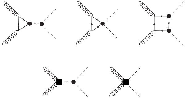
Figure 1: Higgs boson pair production in gluon fusion at leading order in the chiral Lagrangian. The black dots indicate vertices from anomalous couplings present already at leading order in the Lagrangian, the black squares denote effective interactions from contracted loops.

In Ref. Buchalla:2018yce the NLO QCD corrections were calculated within this framework, and NLO results were presented for the twelve benchmark points defined in Ref. Carvalho:2015ttv .

In Ref. Capozi:2019xsi , shapes of the Higgs boson pair invariant mass distribution $m_{hh}$ were analysed in the 5-dimensional space of anomalous couplings using machine learning techniques to classify $m_{hh}$-shapes, starting from NLO predictions. In more detail, $10^{5}$ NLO distributions were produced to train a neural network based on an autoencoder which extracts common shape features, like an enhanced tail or a double peak, in the $m_{hh}$ distribution. Then a KMeans clustering algorithm from scikit-learn scikit was used to identify distinct shape clusters. The aim was to produce clusters that distinguish characteristic shape features without picking on minor details. The cluster centres in the coupling parameter space resulting from this procedure were then associated with candidate benchmark points. However, if the corresponding total cross section exceeded the limit of $6.9\times\sigma_{SM}$ Aad:2019uzh , which is currently the most stringent bound on the total cross section, we proceeded to the parameter point corresponding to the curve next-closest to the cluster center. This method led to seven new benchmark points being identified, which we use here to discuss our phenomenological results. For convenience we repeat the benchmark points in Table 1, together with the corresponding values for the cross section at $\sqrt{s}=14$ TeV.

benchmark	$c_{t}$	$c_{hhh}$	$c_{tt}$	$c_{ggh}$	$c_{gghh}$	$\sigma_{\rm{NLO}}$ [fb]	K-factor	ratio to SM
SM	1	1	0	0	0	32.90 $\pm$ 0.03	1.66	1.00
1	0.94	3.94	-$\frac{1}{3}$	0.5	$\frac{1}{3}$	222.63 $\pm$ 0.12	1.90	6.77
2	0.61	6.84	$\frac{1}{3}$	0.0	-$\frac{1}{3}$	168.13 $\pm$ 0.07	2.14	5.11
3	1.05	2.21	-$\frac{1}{3}$	0.5	0.5	151.94 $\pm$ 0.09	1.83	4.62
4	0.61	2.79	$\frac{1}{3}$	-0.5	$\frac{1}{6}$	63.14 $\pm$ 0.03	2.15	1.92
5	1.17	3.95	-$\frac{1}{3}$	$\frac{1}{6}$	-0.5	154.77 $\pm$ 0.23	1.63	4.70
6	0.83	5.68	$\frac{1}{3}$	-0.5	$\frac{1}{3}$	179.35 $\pm$ 0.18	2.16	5.45
7	0.94	-0.10	1	$\frac{1}{6}$	-$\frac{1}{6}$	131.06 $\pm$ 0.08	2.28	3.98

Table 1: NLO benchmark points derived in Ref. Capozi:2019xsi . The values for the cross section are given at $\sqrt{s}=14$ TeV.

There are different normalisation conventions for the anomalous couplings in the literature. In Table 2 we summarise the conventions commonly used.

Eq. (1), i.e. ${\cal L}$ of Ref. Buchalla:2018yce	Ref. Carvalho:2015ttv	Ref. Grober:2015cwa
$c_{hhh}$	$\kappa_{\lambda}$	$c_{3}$
$c_{t}$	$\kappa_{t}$	$c_{t}$
$c_{tt}$	$c_{2}$	$c_{tt}/2$
$c_{ggh}$	$\frac{2}{3}c_{g}$	$8c_{g}$
$c_{gghh}$	$-\frac{1}{3}c_{2g}$	$4c_{gg}$

Table 2: Translation between the conventions for the definition of the anomalous couplings.

We also give the relation to the corresponding parameters in the SMEFT, using the following Lagrangian based on the counting of canonical dimensions:

$$\Delta{\cal L}_{6} =\frac{\bar{c}_{H}}{2v^{2}}\partial_{\mu}(\phi^{\dagger}\phi)\partial^{\mu}(\phi^{\dagger}\phi)+\frac{\bar{c}_{u}}{v^{2}}y_{t}(\phi^{\dagger}\phi\,\bar{q}_{L}\tilde{\phi}t_{R}+{\rm h.c.})-\frac{\bar{c}_{6}}{2v^{2}}\frac{m^{2}_{h}}{v^{2}}(\phi^{\dagger}\phi)^{3}$$

$$+\frac{\bar{c}_{ug}}{v^{2}}g_{s}(\bar{q}_{L}\sigma^{\mu\nu}G_{\mu\nu}\tilde{\phi}t_{R}+{\rm h.c.})+\frac{4\bar{c}_{g}}{v^{2}}g^{2}_{s}\phi^{\dagger}\phi\,G^{a}_{\mu\nu}G^{a\mu\nu}\;,$$ (2)

where we follow the conventions used in Giudice:2007fh ; Grober:2015cwa , except for $\bar{c}_{g}$ which differs by inclusion of the weak coupling $g^{2}$: $\bar{c}_{g}\Big{|}_{\text{Ref.\cite[cite]{\@@bibref{Authors Phrase1YearPhrase2}{Grober:2015cwa}{\@@citephrase{(}}{\@@citephrase{)}}}}}=g^{2}\,\bar{c}_{g}\Big{|}_{\text{Eq.}(\ref{eq:lsmeft})}$. The term proportional to $\bar{c}_{ug}$ denotes the chromomagnetic operator, which does not contribute at the order in the chiral counting we are considering here ($d\chi\leq 4$), because it gets an additional loop suppression factor $1/16\pi^{2}$ due to the fact that dimension-6 operators involving field strength tensors (such as $\sigma^{\mu\nu}G_{\mu\nu}$) can only be generated through loop diagrams Arzt:1994gp ; Buchalla:2018yce . The remaining coefficients $\bar{c}_{i}$ in Eq. (2) can be related to the couplings of the physical Higgs field $h$ and compared with the corresponding parameters of the chiral Lagrangian (1). After a field redefinition of $h$ to eliminate $\bar{c}_{H}$ from the kinetic term one finds Azatov:2015oxa ; Grober:2015cwa

$$c_{t} =1-\frac{\bar{c}_{H}}{2}-\bar{c}_{u}\;,\;c_{tt}=-\frac{\bar{c}_{H}+3\bar{c}_{u}}{4}\;,\;c_{hhh}=1-\frac{3}{2}\bar{c}_{H}+\bar{c}_{6}\;,$$ (3)

$$c_{ggh} =2c_{gghh}=(16\pi^{2})\times 8\bar{c}_{g}\;.$$ (4)

3 Description of the code

3.1 Structure of the code

The code is an extension of the one presented in Ref. Heinrich:2019bkc to include the possibility of varying all five anomalous couplings rather than only the trilinear Higgs coupling. For the virtual two-loop corrections, we have built on the results of the calculations presented in Refs. Borowka:2016ehy ; Borowka:2016ypz . These results were obtained by performing a (partial) reduction of the two-loop amplitude to master integrals based on Reduze Studerus:2009ye ; vonManteuffel:2012np and a subsequent numerical evaluation of the master integrals using the program SecDec Borowka:2015mxa ; Borowka:2017idc . This has been done with the top quark- and Higgs masses fixed to a numerical value. Therefore these mass values should not be changed in the ggHH code.

The real radiation matrix elements were implemented using the interface between GoSam Cullen:2011ac ; Cullen:2014yla and the POWHEG-BOX Alioli:2010xd ; Luisoni:2013cuh . The extra matrix elements occurring in the EFT framework have been generated by GoSam via a model file in UFO format Degrande:2011ua which has been developed in Ref. Buchalla:2018yce , derived from the effective Lagrangian in Eq. (1) using FeynRules Alloul:2013bka .

The framework presented in Ref. Heinrich:2019bkc to interface the two-loop virtual contribution in POWHEG is generalised in the following way: instead of a second-order polynomial (as for variations of $c_{hhh}$ only), at NLO we can write the squared matrix element for variations of all five anomalous couplings as in Eq. (5), following Refs. Azatov:2015oxa ; Carvalho:2015ttv ; Buchalla:2018yce .

$$|\mathcal{M}_{\rm BSM}|^{2} =a_{1}\,c_{t}^{4}+a_{2}\,c_{tt}^{2}+a_{3}\,c_{t}^{2}c_{hhh}^{2}+a_{4}\,c_{ggh}^{2}c_{hhh}^{2}+a_{5}\,c_{gghh}^{2}+a_{6}\,c_{tt}c_{t}^{2}+a_{7}\,c_{t}^{3}c_{hhh}$$

$$+a_{8}\,c_{tt}c_{t}\,c_{hhh}+a_{9}\,c_{tt}c_{ggh}c_{hhh}+a_{10}\,c_{tt}c_{gghh}+a_{11}\,c_{t}^{2}c_{ggh}c_{hhh}+a_{12}\,c_{t}^{2}c_{gghh}$$

$$+a_{13}\,c_{t}c_{hhh}^{2}c_{ggh}+a_{14}\,c_{t}c_{hhh}c_{gghh}+a_{15}\,c_{ggh}c_{hhh}c_{gghh}\,+a_{16}\,c^{3}_{t}c_{ggh}$$

$$+a_{17}\,c_{t}c_{tt}c_{ggh}+a_{18}\,c_{t}c_{ggh}^{2}c_{hhh}+a_{19}\,c_{t}c_{ggh}c_{gghh}\,+a_{20}\,c_{t}^{2}c_{ggh}^{2}$$

$$+a_{21}\,c_{tt}c_{ggh}^{2}+a_{22}\,c_{ggh}^{3}c_{hhh}+a_{23}\,c_{ggh}^{2}c_{gghh}\,.$$ (5)

For the Born-virtual interference term, we produce grids using 6715 points (5194 points at $\sqrt{s}=14$ TeV and 1521 points at $100$ TeV) for 23 linearly independent sets of couplings. This enables us to derive, for each phase-space point, the coefficients $a_{1},\dots,a_{23}$ by interpolation. Once the user has chosen a set of anomalous couplings, the 23 grids are combined into one using Eq. (5). This step is performed only once, in the first POWHEG parallel stage. The Born and real contributions are evaluated exactly for the chosen anomalous couplings without relying on a grid or interpolation. Note that the $a_{i}$ coefficients of Eq. (5) are not equal to the $A_{i}$ coefficients of Ref. Buchalla:2018yce , which are derived for the (normalised) cross-section and not for the Born-virtual interference term.

The original phase space points were produced with SM couplings, therefore some regions, for example the low $m_{hh}$-region, are less populated than the peak of the $m_{hh}$-distribution in the SM. The statistical uncertainty on the input data induces a systematic uncertainty on the 23 grids. We have checked the relative size of the uncertainties of the virtual corrections in each bin of the $m_{hh}$ distributions for all seven benchmark points. This uncertainty is below 2% throughout the whole $m_{hh}$ range, except for the first bin. This bin is poorly populated in the SM and therefore the uncertainties in this bin are larger for coupling configurations where the low-$m_{hh}$ region is very different from the SM case or where the relative size of the virtual contribution is large. Hence we find uncertainties in the first $m_{hh}$ bin of about 6% for all benchmarks except for benchmark 5, which has a 12% uncertainty in this bin.

3.2 Usage of the code

The code can be found at the web page

http://powhegbox.mib.infn.it

under User-Processes-V2 in the ggHH process directory. An example input card (powheg.input-save) and a run script (run.sh) are provided in the testrun folder accompanying the code.

In the following we only describe the input parameters that are specific to the process $gg\to HH$ including five anomalous couplings. The parameters that are common to all POWHEG-BOX processes can be found in the POWHEG manual V2-paper.pdf in the POWHEG-BOX-V2/Docs directory.

Running modes

The code contains the SM NLO QCD amplitudes with full top quark mass dependence. A detailed description of the different approximations can be found in Ref. Borowka:2016ypz . For the Standard Model case as well as for BSM-values of the trilinear Higgs coupling $c_{hhh}$, the code can be run in four different modes, either by changing the flag mtdep in the POWHEG-BOX run card powheg.input-save, or by using the script run.sh [mtdep mode]. If all five anomalous couplings are varied, there is only the possibility of either calculating at

• NLO with full top quark mass dependence, or

• LO (setting bornonly=1) in either the full theory or in the $m_{t}\to\infty$ limit.

In more detail, the following choices are available:

mtdep=0:

all amplitudes are computed in the $m_{t}\to\infty$ limit (HTL). This option is only available at NLO in the SM case or if only $c_{hhh}$ is varied, or at LO.

mtdep=1:

computation using Born-improved HTL. In this approximation the fixed-order part is computed at NLO in the heavy top limit and reweighted pointwise in the phase-space by the LO matrix element with full mass dependence divided by the LO matrix element in the HTL. This option is only available at NLO in the SM case or if only $c_{hhh}$ is varied, or at LO.

mtdep=2:

computation in the approximation FT_approx. In this approximation the matrix elements for the Born and the real radiation contributions are computed with full top quark mass dependence, whereas the virtual part is computed as in the Born-improved HTL. This option is only available at NLO in the SM case or if only $c_{hhh}$ is varied, or at LO.

mtdep=3:

NLO computation with full top quark mass dependence.

Input parameters

The bottom quark is considered massless in all four mtdep modes. The Higgs bosons are generated on-shell with zero width. A decay can be attached through the parton shower in the narrow-width approximation. However, the decay is by default switched off (see the hdecaymode flag in the example powheg.input-save input card in testrun).

The masses of the Higgs boson and the top quark are set by default to $m_{h}=125$ GeV, $m_{t}=173$ GeV, respectively, and their widths have been set to zero. The full SM two-loop virtual contribution has been computed with these mass values hardcoded, therefore they should not be changed when running with mtdep = 3, otherwise the two-loop virtual part would contain a different top or Higgs mass from the rest of the calculation. It is no problem to change the values of $m_{h}$ and $m_{t}$ via the powheg.input-save input card when running with mtdep set to $0$, $1$ or $2$.

The Higgs couplings as defined in the context of the Electroweak Chiral Lagrangian (see Buchalla:2018yce and references within), can be varied directly in the powheg.input card. These are, with their SM values as default:

chhh=1.0:

the ratio of the Higgs trilinear coupling to its SM value,

ct=1.0:

the ratio of the Higgs Yukawa coupling to the top quark to its SM value,

ctt=0.0:

the effective coupling of two Higgs bosons to a top quark pair,

cggh=0.0:

the effective coupling of two gluons to the Higgs boson,

cgghh=0.0:

the effective coupling of two gluons to two Higgs bosons.

The possibility of varying all Higgs couplings (rather than $c_{hhh}$ only) is only available in the mode mtdep=3 (full NLO). More details about the mtdep=3 running mode are given in Appendix A.1.

The runtimes are dominated by the evaluation of the real radiation part. When run in the full NLO mode, the runtimes we observed were in the ballpark of 100 CPU hrs for an uncertainty of about 0.1% on the total cross section.

4 Phenomenological results

We present results calculated at a centre-of-mass energy of $\sqrt{s}=14$ TeV using the PDF4LHC15_nlo_30_pdfas Butterworth:2015oua ; CT14 ; MMHT14 ; NNPDF parton distribution functions interfaced to our code via LHAPDF Buckley:2014ana , along with the corresponding value for $\alpha_{s}$. The masses of the Higgs boson and the top quark have been fixed to $m_{h}=125$ GeV, $m_{t}=173$ GeV and their widths have been set to zero. The top quark mass is renormalised in the on-shell scheme. Jets are clustered with the anti-$k_{T}$ algorithm Cacciari:2008gp as implemented in the FastJet package Cacciari:2005hq ; Cacciari:2011ma , with jet radius $R=0.4$ and a minimum transverse momentum $p_{T,\mathrm{min}}^{\rm{jet}}=20$ GeV. The scale uncertainties are estimated by varying the factorisation/renormalisation scales $\mu_{F},\mu_{R}$, where the bands represent 3-point scale variations around the central scale $\mu_{0}=m_{hh}/2$, with $\mu_{R}=\mu_{F}=c\,\mu_{0}$, where $c\in\{0.5,1,2\}$. For the case $c_{hhh}=c_{hhh}^{\mathrm{SM}}=1$ we checked that the bands obtained from these variations coincide with the bands resulting from 7-point scale variations.

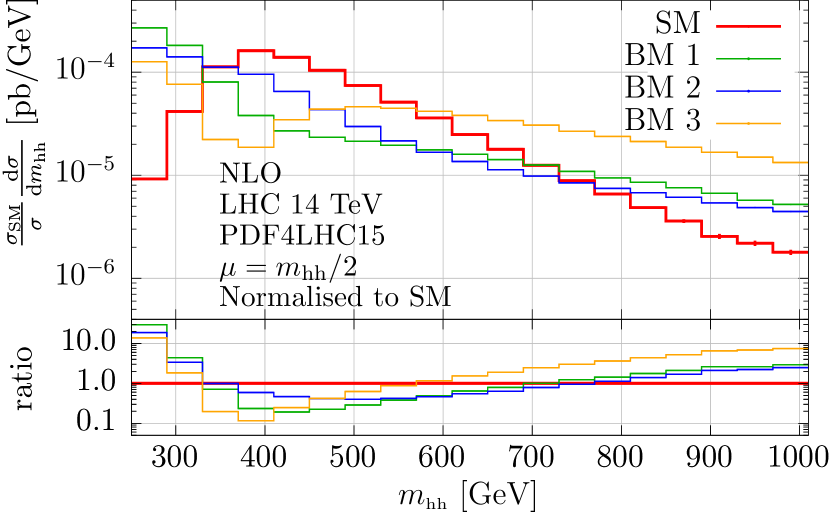
(a)

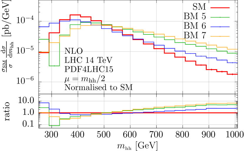
(b)

Figure 2: Normalised Higgs boson pair invariant mass distributions, (a) for benchmark points 1, 2 and 3 compared to the SM, (b) for benchmark points 5, 6 and 7 compared to the SM. All curves are at full NLO. The uncertainties shown are statistical only.

In Fig. 2(a) we show the Higgs boson pair invariant mass distributions for benchmark points 1, 2 and 3 compared to the SM case. The magnitudes of the cross sections are similar, due to the fact that the benchmark points were defined with the constraint that the total cross section should not exceed $6.9\times\sigma_{\rm{SM}}$ at 13 TeV Capozi:2019xsi . Nonetheless, the curves are normalised to the SM cross section, such that only shape differences appear in the figure. Benchmark point 3 has a value of $c_{hhh}$ where the destructive interference between box- and triangle-type contributions is large, which leads to the dip in the $m_{hh}$ spectrum, while the tail is enhanced due to non-zero $c_{ggh}$ and $c_{gghh}$ values. Benchmark point 1 shows the largest enhancement of the very low $m_{hh}$ region, even though its value for $c_{hhh}$ is smaller than the one for benchmark point 2. This behaviour can be attributed to the interplay with the nonzero value of $c_{tt}$, as can be concluded from the analysis in Ref. Capozi:2019xsi .

In Fig. 2(b) the $m_{hh}$ distribution for benchmark points 5, 6 and 7 is shown, normalised to the SM cross section. Benchmark point 5 shows a narrow dip below $m_{hh}=2m_{t}$, which would not be present for $c_{hhh}=3.95$ if all other couplings were SM-like. In fact, from the analysis in Ref. Capozi:2019xsi it can be inferred that the negative $c_{gghh}$ value in combination with $c_{hhh}=3.95$ is causing this dip in the shape.

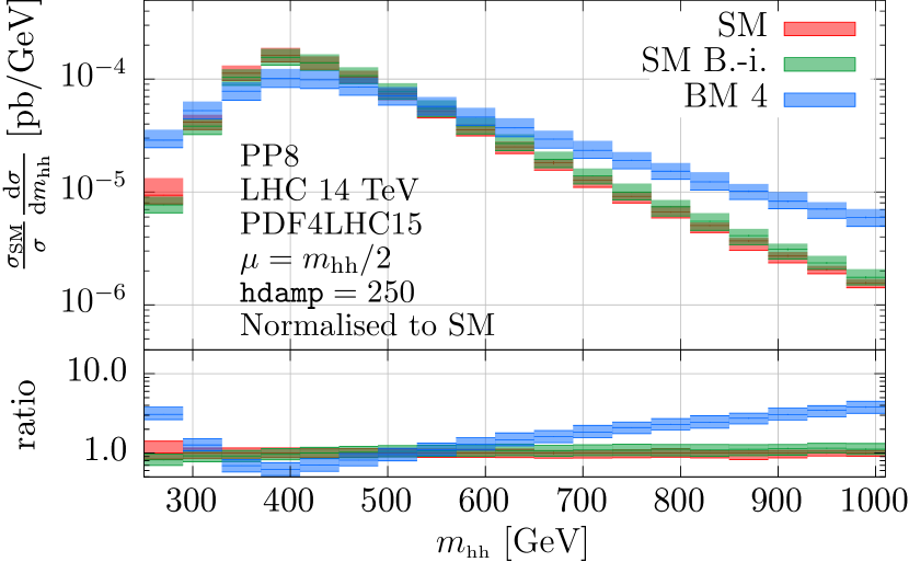
(a)

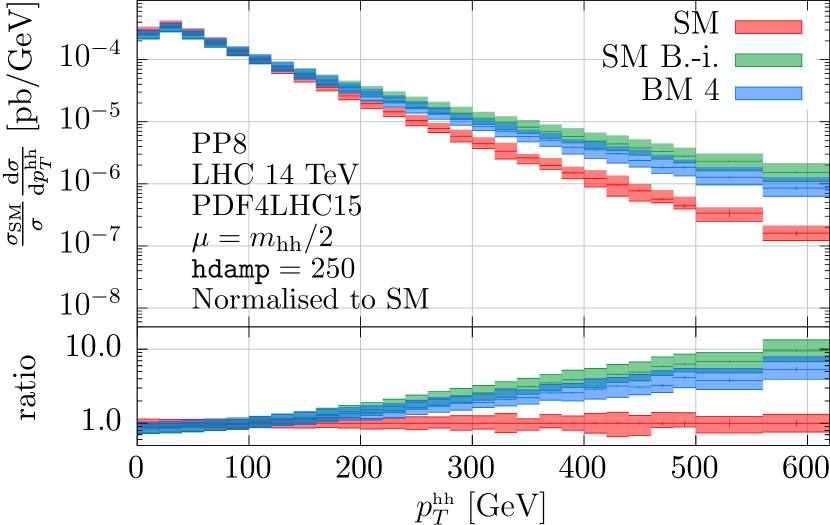
(b)

Figure 3: Normalised distributions for the SM compared to benchmark point 4, both at NLO matched to PYTHIA-8 (PP8). For the SM case, results with the full $m_{t}$-dependence and in the Born-improved (B.-i.) $m_{t}\to\infty$ approximation are shown. (a) Higgs boson pair invariant mass distribution, (b) transverse momentum of the Higgs boson pair.

In Fig. 3(a) we consider benchmark point 4 compared to the full NLO SM as well as in the Born-improved $m_{t}\to\infty$ limit, matched to PYTHIA-8 in all cases. The curves for the Born-improved HTL SM case and for benchmark point 4 are normalised to the SM cross section. Even though the $m_{t}\to\infty$ approximation shows an enhanced tail compared to the full SM, the enhancement of the tail in the case of benchmark 4 is much more pronounced. The situation is different for the $p_{T}^{hh}$ distribution, shown in Fig. 3(b). For this observable, the results for benchmark 4 and the Born-improved $m_{t}\to\infty$ approximation are very close. This fact again shows the importance of the full NLO corrections in order to clearly identify new physics effects.

In both Fig. 3(a) and Fig. 3(b), in order to obtain the scale uncertainty bands, the variation curves were normalised by the ratio of the central-scale prediction to the SM cross section. Thus the bands have the same relative size as in an unnormalised plot. We also investigated a different option to produce the scale bands for the normalised cross section, where the scale uncertainties are not normalised by the ratio $\sigma_{\rm{SM}}/\sigma(\mu_{0})$, but rather by $\sigma_{\rm{SM}}/\sigma(c\,\mu_{0}),\;c\in\{0.5,1,2\}$, i.e. by their own cross section at the considered scale. For the $m_{hh}$ distribution this type of normalisation makes the scale bands disappear within the statistical uncertainties. This is because for central scale choice $\mu_{0}=m_{hh}/2$ the scale variations do not introduce significant shape changes for this observable. For the $p_{T}^{hh}$ distribution the situation is different, firstly because the central scale choice is not aligned with the observable, and secondly because the tail of the $p_{T}^{hh}$ distribution is dominated by $HH$+jet events, which are the leading order in this channel and therefore show larger scale uncertainties. Indeed we observe that when normalised to their own cross-section prediction, the scale uncertainty bands differ from the central prediction by $\pm(3\mbox{-}4)\%$ for $p_{T}^{hh}\lesssim 200$ GeV, and up to $\mp 18\%$ at $p_{T}^{hh}=600$ GeV. This is to be compared to an overall scale uncertainty of $30\mbox{-}40\%$ at $p_{T}^{hh}=600$ GeV with the default normalisation method. To confirm this interpretation, we also investigated scale-varied differential cross sections for the distribution of the transverse momentum of one (any) of the Higgs bosons $p_{T}^{h}$, which is an observable that is not aligned with the choice of scale $\mu=m_{hh}/2$, but which does get contributions from genuine radiative corrections at NLO. When normalised to their own cross section, the scale-varied predictions differ by $\pm 1\%$ from the central prediction at low-to-moderate $p_{T}^{h}$, and grow up to $\mp(8\mbox{-}10)\%$ in the tail at $p_{T}^{h}=600$  GeV. As expected, the scale uncertainties are non-vanishing but still smaller than for the $p_{T}^{hh}$ distribution. In comparison, the full (unnormalised) scale uncertainties are of the order of $\pm(20\mbox{-}25)\%$ across the $p_{T}^{h}$ range.

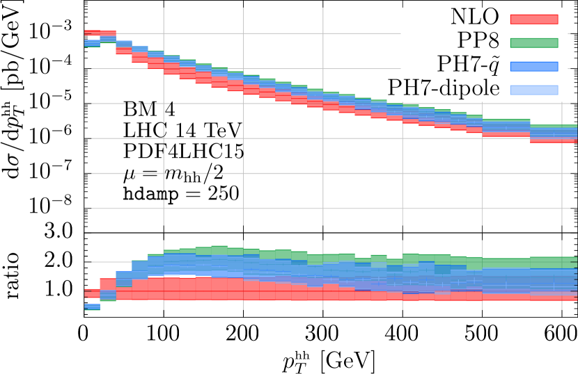
(a)

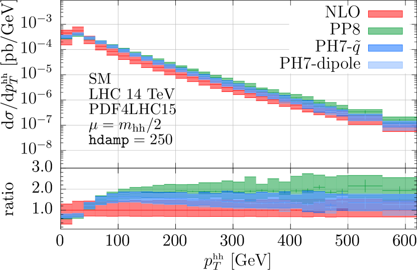
(b)

Figure 4: (a) Transverse momentum of the Higgs boson pair for benchmark point 4, at NLO matched to PYTHIA-8 (PP8) and two different HERWIG-7.2 parton showers (PH7-$\tilde{q}$ and PH7-dipole), compared to the fixed-order result (NLO); (b) same as in (a) but for the SM case.

In Fig. 4 we compare NLO predictions matched to different parton showers, namely PYTHIA-8 and two HERWIG-7.2 parton showers (the angular-ordered $\tilde{q}$ and the dipole shower), to the fixed-order case, (a) for benchmark point 4, and (b) for the SM case. We observe that the enhancement of the tail with POWHEG+PYTHIA-8 present in the SM case is much less pronounced for benchmark 4, where the POWHEG+PYTHIA-8 result also touches onto the fixed-order result at large $p_{T}^{hh}$. This behaviour is most likely due to the non-zero values for $c_{ggh}$ and $c_{gghh}$ for benchmark 4, which cause the tail of the distribution already to be harder than in the SM, such that additional hard radiation created by the shower has a lower relative impact.

5 Conclusions

We have presented a publicly available implementation of Higgs boson pair production in gluon fusion within an Effective Field Theory framework, calculated at full NLO QCD, in the POWHEG-BOX-V2. The code allows five anomalous couplings relevant for di-Higgs production to be varied and offers the possibility to produce fully differential final states.

We have also investigated the behaviour of the shape of the invariant mass distribution of the Higgs boson pair, $m_{hh}$, for seven benchmark points representing characteristic $m_{hh}$-shapes based on an NLO analysis Capozi:2019xsi . In addition, for one of the benchmark points (benchmark 4), characterised by an enhanced tail in the $m_{hh}$ distribution, we carried out a comparison to the full NLO SM result as well as to the $m_{t}\to\infty$ approximation, including scale uncertainties, for both the $m_{hh}$ and the $p_{T}^{hh}$ distributions. We found that the two distributions show different characteristics concerning the distinction of the BSM curve from the SM (and approximate SM) curves: while in the $m_{hh}$ distribution the enhanced tail of benchmark 4 is clearly outside the uncertainty bands of the SM predictions, in the $p_{T}^{hh}$ distribution the bands for benchmark 4 and the SM in the $m_{t}\to\infty$ approximation overlap. This again demonstrates the importance of using full NLO predictions, particularly in trying to resolve partly degenerate directions in the space of anomalous couplings.

We further produced results for the $p_{T}^{hh}$ distribution matched to three different parton showers: PYTHIA-8 and two different HERWIG-7.2 parton showers. The two HERWIG-7.2 parton showers show very similar results. From previous SM results, it is known that loop-induced processes like $gg\to HH$ in POWHEG matched to PYTHIA-8 can show a harder tail than with other parton showers. However, in the case of benchmark point 4, PYTHIA-8 produces less additional hard radiation than in the SM case, such that the PYTHIA-8 and HERWIG-7.2 results are much more similar.

Our studies show that the behaviour of higher-order effects known from the SM does not necessarily carry over to the BSM case, such that precise predictions for both cases are necessary to clearly identify new physics effects. With our code, fully exclusive studies of anomalous couplings in Higgs boson pair production at NLO QCD are possible.

A Appendix

A.1 Running with full top quark mass dependence (mtdep=3)

In this appendix we give some further details about the running mode with full top quark mass dependence.

The two-loop virtual amplitudes in the NLO calculation with full top quark mass dependence are computed via a grid which encodes the dependence of the virtual two-loop amplitude on the kinematic invariants $\hat{s}$ and $\hat{t}$ Heinrich:2017kxx . We emphasize that the numerical values $m_{H}=125$ GeV and $m_{t}=173$ GeV are hardcoded in this grid and therefore should not be changed in powheg.input-save when running in the mtdep=3 mode. The grid is generated using python code and is directly interfaced to the POWHEG-BOX fortran code via a python/C API. In order for the grid to be found by the code, the files (events.cdf, createdgrid.py, Virt_full_*E*.grid) from the folder Virtual need to be copied into the local folder where the code is run. Instead of copying the files, we suggest to create a symbolic link to the needed files. All this is done automatically if you use the script run.sh.

To do this manually: assuming the code is run from a subfolder (e.g. testrun) of the process folder, the link can be created in this subfolder as follows:

ln -s ../Virtual/events.cdf events.cdf

ln -s ../Virtual/creategrid.py creategrid.py

for grid in ../Virtual/Virt_full_*E*.grid; do ln -s $grid; done

Once the links are in place, the code can be run with mtdep=3 as usual. The python code creategrid.py will then combine the virtual grids generated with the 23 combinations of coupling values to produce a new file Virt_full_*E*.grid corresponding to the values of $c_{hhh},c_{t},c_{tt},c_{ggh},c_{gghh}$ defined by the user in the powheg.input-save file.

The python code for the grid relies on the numpy and sympy packages, which the user should install separately. When building the ggHH process the Makefile will find the embedded python 3 library via a call to python3-config, which the user should ensure is configured correctly and points to the correct library. Note that on some systems the python/C API does not search for packages (such as numpy and sympy) in the same paths as the python executable would, the user should ensure that these packages can be found also by an embedded python program. To ensure that the linked files are found, we recommend to add the run subfolder to PYTHONPATH.

A.2 Powheg input and run scripts

The run.sh script in the testrun folder allows the different stages of POWHEG to be run easily. By typing ./run.sh without any argument a menu with the 4 mtdep running modes described above is shown. For all mtdep running modes, run.sh will make the code go through the various steps (parallel stages) of the calculation:

parallelstage=1:

generation of the importance sampling grid for the Monte Carlo integration;

parallelstage=2:

calculation of the integral for the inclusive cross section and an upper bounding function of the integrand;

parallelstage=3:

upper bounding factors for the generation of radiation are computed;

parallelstage=4:

event generation, i.e. production of pwgevents-*.lhe files.

Please note: if you use the script run.sh [mtdep], the value for mtdep given as an argument to run.sh will be used, even if you specified a different value for mtdep in powheg.input-save.

After running parallelstage=4, the LHE files produced by POWHEG can be directly showered by either PYTHIA-8 or HERWIG-7.2. We provide a minimal setup for producing parton-shower matched distributions in test-pythia8, respectively test-herwig7. Both the angular-ordered and the dipole-shower implemented in HERWIG-7.2 can be used by changing the showeralg flag to either default or dipole in HerwigRun.sh.

Further, we should point out that POWHEG offers the possibility to use a damping factor $h=\texttt{hdamp}$ of the form Alioli:2008tz ; Alioli:2009je

$$F=\frac{h^{2}}{(p_{T}^{hh})^{2}+h^{2}}\,,$$ (A.1)

where $p_{T}^{hh}$ is the transverse momentum of the Higgs boson pair, to limit the amount of hard radiation which is exponentiated in the Sudakov form factor. The setting $F\equiv 1$, corresponding to hdamp$=\infty$, results in quite hard tails for observables like $p_{T}^{hh}$ Heinrich:2017kxx ; Heinrich:2019bkc . Changing the damping factor $F$ by setting the flag hdamp to some finite value in the input card softens the high transverse momentum tails. Varying hdamp allows shower uncertainties to be assessed within the POWHEG matching scheme. However, hdamp should not be so low that it starts to cut into the Sudakov regime. In fact, a too low value for hdamp could spoil the logarithmic accuracy of the prediction. For this reason we suggest not to choose values for hdamp below $\sim 200$. Our default value is hdamp=250.

References

- (1) ATLAS collaboration, G. Aad et al., Combined measurements of Higgs boson production and decay using up to fb-1 of proton-proton collision data at 13 TeV collected with the ATLAS experiment, Phys. Rev. D101 (2020) 012002 [1909.02845].
- (2) CMS collaboration, A. M. Sirunyan et al., Measurement and interpretation of differential cross sections for Higgs boson production at 13 TeV, Phys. Lett. B792 (2019) 369 [1812.06504].
- (3) CMS collaboration, A. M. Sirunyan et al., Combination of searches for Higgs boson pair production in proton-proton collisions at 13 TeV, Phys. Rev. Lett. 122 (2019) 121803 [1811.09689].
- (4) ATLAS collaboration, G. Aad et al., Combination of searches for Higgs boson pairs in collisions at 13 TeV with the ATLAS detector, Phys. Lett. B800 (2020) 135103 [1906.02025].
- (5) O. J. P. Eboli, G. C. Marques, S. F. Novaes and A. A. Natale, Twin Higgs Boson Production, Phys. Lett. B197 (1987) 269.
- (6) E. W. N. Glover and J. J. van der Bij, Higgs Boson Pair Production via Gluon Fusion, Nucl. Phys. B309 (1988) 282.
- (7) T. Plehn, M. Spira and P. M. Zerwas, Pair production of neutral Higgs particles in gluon-gluon collisions, Nucl. Phys. B479 (1996) 46 [hep-ph/9603205].
- (8) S. Borowka, N. Greiner, G. Heinrich, S. P. Jones, M. Kerner, J. Schlenk et al., Higgs Boson Pair Production in Gluon Fusion at Next-to-Leading Order with Full Top-Quark Mass Dependence, Phys. Rev. Lett. 117 (2016) 012001 [1604.06447].
- (9) S. Borowka, N. Greiner, G. Heinrich, S. P. Jones, M. Kerner, J. Schlenk et al., Full top quark mass dependence in Higgs boson pair production at NLO, JHEP 10 (2016) 107 [1608.04798].
- (10) J. Baglio, F. Campanario, S. Glaus, M. Mühlleitner, M. Spira and J. Streicher, Gluon fusion into Higgs pairs at NLO QCD and the top mass scheme, Eur. Phys. J. C79 (2019) 459 [1811.05692].
- (11) J. Baglio, F. Campanario, S. Glaus, M. Mühlleitner, J. Ronca, M. Spira et al., Higgs-Pair Production via Gluon Fusion at Hadron Colliders: NLO QCD Corrections, JHEP 04 (2020) 181 [2003.03227].
- (12) G. Heinrich, S. P. Jones, M. Kerner, G. Luisoni and E. Vryonidou, NLO predictions for Higgs boson pair production with full top quark mass dependence matched to parton showers, JHEP 08 (2017) 088 [1703.09252].
- (13) S. Jones and S. Kuttimalai, Parton Shower and NLO-Matching uncertainties in Higgs Boson Pair Production, JHEP 02 (2018) 176 [1711.03319].
- (14) G. Heinrich, S. P. Jones, M. Kerner, G. Luisoni and L. Scyboz, Probing the trilinear Higgs boson coupling in di-Higgs production at NLO QCD including parton shower effects, JHEP 06 (2019) 066 [1903.08137].
- (15) S. Dawson, S. Dittmaier and M. Spira, Neutral Higgs boson pair production at hadron colliders: QCD corrections, Phys. Rev. D58 (1998) 115012 [hep-ph/9805244].
- (16) F. Maltoni, E. Vryonidou and M. Zaro, Top-quark mass effects in double and triple Higgs production in gluon-gluon fusion at NLO, JHEP 11 (2014) 079 [1408.6542].
- (17) D. de Florian and J. Mazzitelli, Two-loop virtual corrections to Higgs pair production, Phys. Lett. B724 (2013) 306 [1305.5206].
- (18) D. de Florian and J. Mazzitelli, Higgs Boson Pair Production at Next-to-Next-to-Leading Order in QCD, Phys. Rev. Lett. 111 (2013) 201801 [1309.6594].
- (19) J. Grigo, K. Melnikov and M. Steinhauser, Virtual corrections to Higgs boson pair production in the large top quark mass limit, Nucl. Phys. B888 (2014) 17 [1408.2422].
- (20) D. de Florian, M. Grazzini, C. Hanga, S. Kallweit, J. M. Lindert, P. Maierhöfer et al., Differential Higgs Boson Pair Production at Next-to-Next-to-Leading Order in QCD, JHEP 09 (2016) 151 [1606.09519].
- (21) M. Grazzini, G. Heinrich, S. Jones, S. Kallweit, M. Kerner, J. M. Lindert et al., Higgs boson pair production at NNLO with top quark mass effects, JHEP 05 (2018) 059 [1803.02463].
- (22) D. De Florian and J. Mazzitelli, Soft gluon resummation for Higgs boson pair production including finite Mt effects, JHEP 08 (2018) 156 [1807.03704].
- (23) L.-B. Chen, H. T. Li, H.-S. Shao and J. Wang, Higgs boson pair production via gluon fusion at N3LO in QCD, Phys. Lett. B803 (2020) 135292 [1909.06808].
- (24) L.-B. Chen, H. T. Li, H.-S. Shao and J. Wang, The gluon-fusion production of Higgs boson pair: N3LO QCD corrections and top-quark mass effects, JHEP 03 (2020) 072 [1912.13001].
- (25) S. Amoroso et al., Les Houches 2019: Physics at TeV Colliders: Standard Model Working Group Report, in 11th Les Houches Workshop on Physics at TeV Colliders: PhysTeV Les Houches (PhysTeV 2019) Les Houches, France, June 10-28, 2019, 2020, 2003.01700.
- (26) M. Cepeda et al., Report from Working Group 2, CERN Yellow Rep. Monogr. 7 (2019) 221 [1902.00134].
- (27) J. Alison et al., Higgs Boson Pair Production at Colliders: Status and Perspectives, in Double Higgs Production at Colliders Batavia, IL, USA, September 4, 2018-9, 2019 (B. Di Micco, M. Gouzevitch, J. Mazzitelli and C. Vernieri, eds.), 2019, 1910.00012, https://lss.fnal.gov/archive/2019/conf/fermilab-conf-19-468-e-t.pdf.
- (28) S. Dawson, C. Englert and T. Plehn, Higgs Physics: It ain’t over till it’s over, Phys. Rept. 816 (2019) 1 [1808.01324].
- (29) G. Buchalla, M. Capozi, A. Celis, G. Heinrich and L. Scyboz, Higgs boson pair production in non-linear Effective Field Theory with full -dependence at NLO QCD, JHEP 09 (2018) 057 [1806.05162].
- (30) P. Nason, A New method for combining NLO QCD with shower Monte Carlo algorithms, JHEP 11 (2004) 040 [hep-ph/0409146].
- (31) S. Frixione, P. Nason and C. Oleari, Matching NLO QCD computations with Parton Shower simulations: the POWHEG method, JHEP 11 (2007) 070 [0709.2092].
- (32) S. Alioli, P. Nason, C. Oleari and E. Re, A general framework for implementing NLO calculations in shower Monte Carlo programs: the POWHEG BOX, JHEP 06 (2010) 043 [1002.2581].
- (33) M. Capozi and G. Heinrich, Exploring anomalous couplings in Higgs boson pair production through shape analysis, JHEP 03 (2020) 091 [1908.08923].
- (34) T. Sjöstrand, S. Ask, J. R. Christiansen, R. Corke, N. Desai, P. Ilten et al., An Introduction to PYTHIA 8.2, Comput. Phys. Commun. 191 (2015) 159 [1410.3012].
- (35) J. Bellm et al., Herwig 7.1 Release Note, 1705.06919.
- (36) R. Alonso, M. B. Gavela, L. Merlo, S. Rigolin and J. Yepes, The Effective Chiral Lagrangian for a Light Dynamical ”Higgs Particle”, Phys. Lett. B722 (2013) 330 [1212.3305].
- (37) G. Buchalla, O. Cata and C. Krause, Complete Electroweak Chiral Lagrangian with a Light Higgs at NLO, Nucl. Phys. B880 (2014) 552 [1307.5017].
- (38) G. Buchalla, O. Cata and C. Krause, On the Power Counting in Effective Field Theories, Phys. Lett. B731 (2014) 80 [1312.5624].
- (39) A. Carvalho, M. Dall’Osso, T. Dorigo, F. Goertz, C. A. Gottardo and M. Tosi, Higgs Pair Production: Choosing Benchmarks With Cluster Analysis, JHEP 04 (2016) 126 [1507.02245].
- (40) https://www.scikit-learn.org.
- (41) R. Gröber, M. Mühlleitner, M. Spira and J. Streicher, NLO QCD Corrections to Higgs Pair Production including Dimension-6 Operators, JHEP 09 (2015) 092 [1504.06577].
- (42) G. Giudice, C. Grojean, A. Pomarol and R. Rattazzi, The Strongly-Interacting Light Higgs, JHEP 06 (2007) 045 [hep-ph/0703164].
- (43) C. Arzt, M. B. Einhorn and J. Wudka, Patterns of deviation from the standard model, Nucl. Phys. B433 (1995) 41 [hep-ph/9405214].
- (44) A. Azatov, R. Contino, G. Panico and M. Son, Effective field theory analysis of double Higgs boson production via gluon fusion, Phys. Rev. D92 (2015) 035001 [1502.00539].
- (45) C. Studerus, Reduze-Feynman Integral Reduction in C++, Comput. Phys. Commun. 181 (2010) 1293 [0912.2546].
- (46) A. von Manteuffel and C. Studerus, Reduze 2 - Distributed Feynman Integral Reduction, 1201.4330.
- (47) S. Borowka, G. Heinrich, S. P. Jones, M. Kerner, J. Schlenk and T. Zirke, SecDec-3.0: numerical evaluation of multi-scale integrals beyond one loop, Comput. Phys. Commun. 196 (2015) 470 [1502.06595].
- (48) S. Borowka, G. Heinrich, S. Jahn, S. P. Jones, M. Kerner, J. Schlenk et al., pySecDec: a toolbox for the numerical evaluation of multi-scale integrals, Comput. Phys. Commun. 222 (2018) 313 [1703.09692].
- (49) G. Cullen, N. Greiner, G. Heinrich, G. Luisoni, P. Mastrolia, G. Ossola et al., Automated One-Loop Calculations with GoSam, Eur. Phys. J. C72 (2012) 1889 [1111.2034].
- (50) G. Cullen et al., GS-2.0: a tool for automated one-loop calculations within the Standard Model and beyond, Eur. Phys. J. C74 (2014) 3001 [1404.7096].
- (51) G. Luisoni, P. Nason, C. Oleari and F. Tramontano, /HZ + 0 and 1 jet at NLO with the POWHEG BOX interfaced to GoSam and their merging within MiNLO, JHEP 1310 (2013) 083 [1306.2542].
- (52) C. Degrande, C. Duhr, B. Fuks, D. Grellscheid, O. Mattelaer and T. Reiter, UFO - The Universal FeynRules Output, Comput. Phys. Commun. 183 (2012) 1201 [1108.2040].
- (53) A. Alloul, N. D. Christensen, C. Degrande, C. Duhr and B. Fuks, FeynRules 2.0 - A complete toolbox for tree-level phenomenology, Comput. Phys. Commun. 185 (2014) 2250 [1310.1921].
- (54) J. Butterworth et al., PDF4LHC recommendations for LHC Run II, J. Phys. G43 (2016) 023001 [1510.03865].
- (55) S. Dulat, T.-J. Hou, J. Gao, M. Guzzi, J. Huston, P. Nadolsky et al., New parton distribution functions from a global analysis of quantum chromodynamics, Phys. Rev. D93 (2016) 033006 [1506.07443].
- (56) L. A. Harland-Lang, A. D. Martin, P. Motylinski and R. S. Thorne, Parton distributions in the LHC era: MMHT 2014 PDFs, Eur. Phys. J. C75 (2015) 204 [1412.3989].
- (57) NNPDF collaboration, R. D. Ball et al., Parton distributions for the LHC Run II, JHEP 04 (2015) 040 [1410.8849].
- (58) A. Buckley, J. Ferrando, S. Lloyd, K. Nordström, B. Page, M. Rüfenacht et al., LHAPDF6: parton density access in the LHC precision era, Eur. Phys. J. C75 (2015) 132 [1412.7420].
- (59) M. Cacciari, G. P. Salam and G. Soyez, The anti- jet clustering algorithm, JHEP 04 (2008) 063 [0802.1189].
- (60) M. Cacciari and G. P. Salam, Dispelling the myth for the jet-finder, Phys.Lett. B641 (2006) 57 [hep-ph/0512210].
- (61) M. Cacciari, G. P. Salam and G. Soyez, FastJet User Manual, Eur.Phys.J. C72 (2012) 1896 [1111.6097].
- (62) S. Alioli, P. Nason, C. Oleari and E. Re, NLO Higgs boson production via gluon fusion matched with shower in POWHEG, JHEP 04 (2009) 002 [0812.0578].
- (63) S. Alioli, P. Nason, C. Oleari and E. Re, NLO single-top production matched with shower in POWHEG: s- and t-channel contributions, JHEP 09 (2009) 111 [0907.4076].