PriorGAN: Real Data Prior for Generative Adversarial Nets

Abstract

Generative adversarial networks (GANs) have achieved rapid progress in learning rich data distributions. However, we argue about two main issues in existing techniques. First, the low quality problem where the learned distribution has massive low quality samples. Second, the missing modes problem where the learned distribution misses some certain regions of the real data distribution. To address these two issues, we propose a novel prior that captures the whole real data distribution for GANs, which are called PriorGANs. To be specific, we adopt a simple yet elegant Gaussian Mixture Model (GMM) to build an explicit probability distribution on the feature level for the whole real data. By maximizing the probability of generated data, we can push the low quality samples to high quality. Meanwhile, equipped with the prior, we can estimate the missing modes in the learned distribution and design a sampling strategy on the real data to solve the problem. The proposed real data prior can generalize to various training settings of GANs, such as LSGAN, WGAN-GP, SNGAN, and even the StyleGAN. Our experiments demonstrate that PriorGANs outperform the state-of-the-art on the CIFAR-10, FFHQ, LSUN-cat, and LSUN-bird datasets by large margins.

1 Introduction

Generative Adversarial Networks (GANs) [8] have achieved great success in learning high dimensional probability distributions. The capability of GANs advances many important and useful applications, like high quality image generation [15, 4], image-to-image translation [14, 33], image editing [23, 9], and so on. However, GANs still suffer from the unstable training process.

Many recent works [24, 19, 2, 10, 20] focus on stabilizing the training process of GANs. Despite their success, there are still two main issues in current GANs. First, the learned distribution always contains massive low quality samples. We refer to this phenomenon as the low quality problem. Second, the learned distribution misses certain areas of real data distribution. We refer to this phenomenon as the missing modes (also known as mode dropping) problem. We have carefully studied these two problems and observed that they may be caused by the inaccurate gradient direction from the discriminator.

Ideally, the gradient direction of the discriminator to the generator will make the generated data distribution as close to the real data distribution as possible. However, we found that in practice, the discriminator cannot achieve the theoretical optimal point due to insufficient iteration number or limited fitting ability. In this situation, the gradient direction given by the discriminator is sometimes inaccurate. Previous methods [10, 20] try to solve the inaccurate gradient problem with the Lipschitz constraint for the discriminator. But the Lipschitz constraint will further limit the capability of the discriminator so that it still can not provide accurate gradient for the generated data. More recent work LGAN [39] proved that penalizing Lipschitz constant guarantees the gradient for generated data is accurate, but it requires the discriminator need to be optimal before each iteration of generator training, which is impractical for GANs training.

To address these issues, we adopt an auxiliary model to help the generated data get the accurate gradient direction. We propose to build an explicitly prior to the real data distribution for GANs, which we call PriorGANs. Specifically, we choose to adopt the Gaussian Mixture Model (GMM) to establish a probabilistic model for the real data distribution. Equipped with this model, we can address both issues. For the low quality issue, we can apply the model to estimate the probability of each generated image, the probability can also indicate image quality. By encouraging the low quality samples to get a higher probability in the model, low quality samples will get a gradient direction to the real data nearby. Therefore the low quality problem could be solved. We call this the quality loss.

For the missing modes issue, we can take full advantage of the GMM model to divide the real data into several groups. Each group may represent a specific mode. Then we can get the densities of the real data in each group. During the training process of GANs, we can estimate the densities of the generated data in each group. If the density of generated data in a group is lower (or higher) than real data, we will increase (or decrease) the sampling frequency of the real data in that group for the next training iteration. We call this the resampling strategy. It will help the generative model solve the missing modes problem.

The proposed PriorGAN is simple, flexible, and general. Our experiments demonstrate that it is suitable for various types of GANs, and it outperforms state-of-the-art GAN frameworks, including LSGAN, WGAN-GP, SNGAN and StyleGAN, on CIFAR-10, FFHQ, LSUN-cat and LSUN-bird datasets by large margins.

In summary, our key contributions are:

1. We demonstrate the low quality and missing modes problems in current GANs and demonstrate the cause of these two problems on toy examples.

2. We propose real data prior for GANs(PriorGANs), equipped with the prior, we propose the quality loss and resampling strategy help current GANs solve these problems.

3. Our experiments demonstrate that PriorGANs outperform state-of-the-art GAN frameworks on various datasets by large margins.

2 Related Work

Over the past years, GANs have achieved significant attention in the deep learning community. Massive works are proposed to improve the performance of GANs. In this section, we will briefly review them. Also, we will review some classical algorithms about modeling data distribution.

Generative Adversarial Nets. Early works about GANs try to solve the unstable training process of GANs, many works focus on proposing new loss functions to solve this problem. For example, LSGAN [19] replace the original BCE loss with the proposed least square loss. WGAN [2] proposes the Wasserstein distance and weight clipping to achieve the Lipschitz condition. Later work began to notice the Lipschitz condition. Some typical works are as follows: WGAN-GP [2] further introduce the gradient penalty to achieve the Lipschitz condition. SNGAN [20] proposes Spectral Normalization to achieve Lipschitz condition for training GANs. More recent works [7, 21, 5] design task-specific loss functions for GANs. Meanwhile, some works aim to improve the diversity of the GANs, for instance, VEEGAN [28] and CVAE-GAN [3] proposes to reconstruct the images in the pixel level to avoid the missing modes problems. MS-GAN [18] proposes a loss term that maximizes the ratio of the distance between generated images with respect to the corresponding latent codes. Besides new loss functions, there are also some works [24, 15, 38, 16] focus on using different network structures and training strategies for training. In contrast to these methods, our method proposes to build explicit real data prior to solving these problems.

Build Prior for Data Distribution. There are various methods that aim to build the prior for underlying data distribution. For example, Principle Component Analysis (PCA)  [32], Independent Component Analysis (ICA) [13], and the Gaussian Mixture Model (GMM) [35, 26], all assume the data distribution follow a simple assumption. But they have difficulty modeling complex patterns of irregular distributions. Later works, such as the Hidden Markov Model (HMM) [29], Markov Random Field (MRF) [25], and restricted Boltzmann machines (RBMs) [27]. limiting their results on texture patches, digital numbers, due to a lack of effective feature representations. Instead of building the model directly on the pixel space, we leverage the successful feature presentation of the CNNs [11, 30] and build the model on these feature representations.

3 Methods

Before we introduce our methods, we first give a brief introduction and our findings about current GANs. In the vanilla GAN, the discriminator D and the generator G play the following two-player minimax game with value function $V(D,G)$:

$$\min_{G}\max_{D}V(D,G)=\mathbb{E}_{x\sim p_{\text{r}}(x)}[\log D(x)]+\mathbb{E}_{x\sim G(z)}[\log(1-D(x))].$$ (1)

suppose $p_{g}(x)=G(z)$, for G fixed, the optimal discriminator $D$ for $V(D,G)$ is:

$$D^{*}_{G}(\bm{x})=\frac{p_{\text{r}}(x)}{p_{\text{r}}(x)+p_{g}(x)}$$ (2)

According to the analysis in GAN [8], the global minimum of $V(D^{*}_{G},G)$ is achieved if and only if $p_{g}=p_{r}$. But in the practical training process of GAN, the optimal discriminator $D_{G}^{*}(x)$ is usually hard to achieve due to insufficient training iterations or limited network capability. In this situation, the gradient is probably incorrect for reaching the optimal $p_{g}$.

To demonstrate this, we train a basic GAN [8] on two typical toy distributions. As illustrated in Figure 1, The green points are the real data, the blue points are the generated data, the discriminator is trained based on current real and generated data distribution. The red arrows denote the gradient of the discriminator for each generated data. In Figure 1(a), some generated data are out of the real data distribution. But the gradients of these low quality generated points are not correct and they can’t move to the real data distribution. So these samples stay in the situation of low quality problem. In Figure 1(c), we notice that the real data distribution has two main regions, but the gradient of the generated points have the same direction to one region of the real data. This seems to be an intrinsic cause of the missing modes problem.

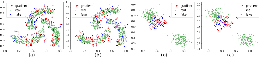
Figure 1: An example of low quality problem(a,b) and missing modes problem(c,d) in GANs training on toy examples, (a) and (c) show the gradient of vanilla GAN, (b) and (d) show the gradient of our proposed PriorGAN.

To solve these problems, we propose to establish a prior model on real data to help the discriminator solve the inaccurate gradient problem. Equipped with the prior, we can solve the problem of low quality and missing modes. In the next section, we will first introduce how to build real data prior. Then we present how to apply the prior as a loss term in GAN training to improve the quality of generated images. After that, we show how to use this prior to estimate the diversity of the real and generated data distribution. Finally, we introduce the resampling strategy to improve the diversity of the generated samples.

3.1 Build Prior for Real Data

Building an explicit prior to the high dimensional data is very difficult and challenging, especially for high-resolution images. This is because the real data distribution is extremely complicated to be captured by a simple prior. Previous method [26] try to leverage the Gaussian Mixture Model(GMM) model to build a model on the image patch level. However, the image resolution is restricted to be very small and the generated results are really blurry. Instead of directly building the GMM model on the pixel level, we take full advantage of the recent success of deep convolutional networks and build the GMM model on the features extracted by the networks. The deep feature is suitable for building the GMM model from two aspects. First, the deep feature is relatively low dimensional, which helps avoid the overfitting problem. Second, the deep feature is very representative and explicitly represents the content of the image. Denote the input image as $x$, the deep feature extractor function as $F(\cdot)$. We use a pre-trained network as feature extractor and the extracted feature dimension is $d$. Suppose the GMM model has $M$ Gaussian components, the mean vector and covariance matrix for $i$-th Gaussian component are $\mu_{i}$ and $\Sigma_{i}$, respectively. Given these parameters, the density function of a Gaussian Mixture Model takes the form

$$p(x|\lambda)=\sum_{i=1}^{M}w_{i}\mathcal{N}(F(x)|\mu_{i},\Sigma_{i}),x\in P_{r}$$ (3)

$P_{r}$ denotes real image space, $w_{i}$ is the mixture weights, which satisfy the constraint that $\sum_{i=1}^{M}w_{i}=1$. And $\mathcal{N}(F(x)|\mu_{i},\Sigma_{i})$ is a $d$-variate Gaussian function of the form. The complete Gaussian mixture model is parameterized by the mean vectors, covariance matrices and mixture weights from all component densities. These parameters are collectively represented by the notation, $\lambda=\{w_{i},\mu_{i},\Sigma_{i}\}$. To estimate these parameters, we adopt the expectation-maximization (EM) algorithm [6] to iteratively update them with the loss function

$$L=\sum_{x\in P_{r}}-\log p(x|\lambda).\vspace{-0.2cm}$$ (4)

3.2 Improving Quality with Prior

Given the estimated GMM model, for a generated image $x\in P_{g}$, we can adopt $p(\mathbf{x}|\lambda)$ in Equation. 3 to estimate its probability. If its probability is high, it indicates that it is close to some of the real samples and the quality is high, otherwise, it is far from real samples and the quality is poor. So the generator should pay more attention to these poor quality samples. However, previous analysis shows that these poor quality generated samples may get inaccurate gradient from the discriminator. To solve this problem, we propose to utilize the prior to restrict these poor quality samples to get a higher probability in the built GMM model. This will help the poor quality samples to have an accurate gradient direction towards the real data distribution. Formally, given an generated image $x=G(z)$, $G$ is the generator, the loss for the generator is:

$$\mathcal{L}_{Q}=\begin{cases}-\log p(F(G(z))|\lambda)&\textit{if }p(F(G(z))|\lambda)<\theta\\ 0&\textit{otherwise}\end{cases},$$ (5)

where $\theta$ is the quality threshold. The quality loss $\mathcal{L}_{Q}$ mainly focuses on the low quality generated results and will give a right gradient direction for these low quality generated samples, as illustrated in Figure 1(b). During the training process of GANs, we give a loss weight $\delta$ to this quality loss and apply it as an auxiliary term to update the generator besides the GAN loss.

3.3 Improving Diversity with Prior

Current GANs often suffer from the missing modes problem, the learned distribution from GANs may miss some certain regions of the real data distribution. Therefore the key is how we can estimate the diversity of real data distribution and find these missing regions in the learned distribution. One possible solution is to apply the built GMM model. Specifically, if we establish a GMM model to represent a real data distribution, then we can apply the $M$ Gaussian components in the GMM model to divide the real data distribution into $M$ groups and estimate the frequency of the real samples in each group. A sample belonging to which Gaussian component is decided by the minimum distance to the center of each Gaussian component, as we shown in Figure 2. Suppose the number of the real samples on the $i$-th Gaussian component is $n_{i}^{r}$, then the frequency of the real samples on the $i$-th Gaussian component is $f_{i}^{r}={n_{i}^{r}}/{\sum_{i}^{M}{n_{i}^{r}}}$. And we have the vector $[f_{1}^{r},f_{2}^{r},\cdots,f_{M}^{r}]$ to represent the diversity of the real samples. Similarly, we apply the same GMM model to get the frequency of generated samples, which is denoted as $[f_{1}^{g},f_{2}^{g},\cdots,f_{M}^{g}]$.

Figure 2: Visualization of learned GMM-based prior on FFHQ and LSUN-cat dataset, each column are images randomly selected from the same Gaussian component. We can observe that images within the same Gaussian component share the same attributes, like hat, hair, sunglasses for the FFHQ or eyes, color, posture for the LSUN-cat.

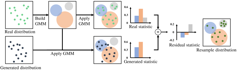
Figure 3: illustration of the pipeline of our resampling strategy.

The frequency difference between the real and generated samples can indicate whether the missing modes problem occurs. If the learned distribution misses a certain region $S$ of the real data distribution, and $S$ belongs to the $i$-th Gaussian component of the built GMM model, then $i$-th learned data frequency $f_{i}^{g}$ will be smaller than the real data frequency $f_{i}^{r}$. So the diversity difference between real data distribution and learned distribution can be represented by the frequency distances. Suppose the diversity distance between real data distribution $p_{r}$ and learned distribution $p_{g}$ is denoted as

$$d(p_{r},p_{g})=[f_{1}^{r},f_{2}^{r},\cdots,f_{M}^{r}]-[f_{1}^{g},f_{2}^{g},\cdots,f_{M}^{g}].$$ (6)

So $d(p_{r},p_{g})$ is a vector with $M$ elements, the $i$-th element is $d_{i}(p_{r},p_{g})$. So the overall diversity differences score (DDS) is

$$DDS(p_{r},p_{g})=\sum_{i}^{M}|d_{i}(p_{r},p_{g})|.$$ (7)

An ideal learned distribution should satisfy $DDS(p_{r},p_{g})=0$. However, the $DDS$ is non-differentiable and cannot be directly used as a loss function. So we optimize it in an indirect way and proposed a resampling strategy. Considering a typical missing modes phenomenon where the real data distribution has two regions $S_{1}$ and $S_{2}$, the generated samples only lies around the $S_{1}$, current discriminator can’t force the generated samples around $S_{1}$ to move to $S_{2}$ since the discriminator consider the generated samples around $S_{1}$ are "real enough". To overcome this problem, we propose to change the decision boundary of the discriminator. If we sample fewer samples in $S_{1}$ and more samples in $S_{2}$ for training the discriminator, the decision boundary of the discriminator will be changed. The discriminator will encourage the generated samples to move to $S_{2}$ and solve the missing modes problem, as illustrated in Figure 1(d). We call this process the resampling strategy. This strategy will change the real data distribution in the training procedure to help the generator overcome the missing modes problem. Formally, we use a new sampling frequency $f^{r^{\prime}}_{i}$ to sample the real samples in the $i$-th Gaussian component for training. $f^{r^{\prime}}_{i}$ is decided by the original frequency and the diversity distances:

$$f^{r^{\prime}}_{i}=max(f_{i}^{r}+\alpha d_{i}(p_{r},p_{g}),0),$$ (8)

Then we normalized the sampling frequency, $f^{r^{\prime}}_{i}={f^{r^{\prime}}_{i}}/{\sum_{i}^{M}f^{r^{\prime}}_{i}}$. Such that the new sampling frequency is between $0$ and $1$, $\alpha$ is a hyper parameter which decides the resample weight. For $f_{g}^{i}<f_{r}^{i}$, we increase the sampling frequency of region $i$ and decrease it if otherwise. The resampling strategy is also illustrated in Figure 3.

Above we introduce our methods for improving quality and diversity with our proposed prior. This prior can be integrated into various frameworks of GANs, such as WGAN-GP [10], LSGAN [19], SNGAN [20], and even the StyleGAN [16]. This flexible combination with existing methods can help these methods get further improvement.

4 Experiments

In this part, we conduct experiments on a large variety of generative models trained on different datasets including CIFAR-10 [17], LSUN [37], and FFHQ [16] datasets to evaluate the performance of our proposed methods.

Datasets. CIFAR-10 is a widely used dataset for image generation. We directly apply the original image size $32\times 32$ for training. LSUN [37] is widely used for high-resolution image generation, we choose two categories in LSUN for training and evaluation: cat and bird, which we call LSUN-cat and LSUN-bird, respectively. LSUN-cat contains $1.6$ million images and LSUN-bird contains $2.2$ million images, we follow the settings in StyleGAN [16] to resize all the images to $256\times 256$ resolution. FFHQ [16] is a recently high-resolution face dataset contains $70000$ images, we resize them to $256\times 256$ resolution for training, which we call FFHQ-256.

Evaluations. To evaluate the quality of an image set, as we mentioned earlier, the probability of each image in our GMM model can indicate its quality. So we use the mean of normalized image density in Equation 3 to evaluate the quality of an image set, calculated as: $\frac{1}{K}\sum_{\mathbf{i}=1}^{K}norm(log(p(x_{i}|\lambda)))$, $K$ is the number of images in the image set. We named it Quality Score(QS), higher QS indicates better image quality. And we use our proposed DDS to evaluate the diversity of the generative model, FID [12] to measure both quality and diversity. For a fair comparison, we would use $5k$ or $50k$ genearted images to calculate the FID, denoted as FID(5K) and FID(50K) respectively. $10k$ images are used to calculate QS and DDS for the CIFAR-10 dataset. For the FFHQ, LSUN-cat, and LSUN-bird datasets, we use $50k$ images to calculate the result of the FID, QS and DDS.

Implementation Details. For each baseline, we follow training settings in their experiments. We only add quality loss and the resampling strategy during the training of each baseline. In order to build the prior for each dataset, we apply ResNet101 [11] or InceptionV3 [30] to extract the features for all the real images. The features we use are from the last average pooling layer. Without special notes, we use ResNet101 to extract the features. Then we build the prior for each dataset. Specifically, we set the number of Gaussian component to $35$,$70$, $7$, and $7$, the resample weight $\alpha$ to $3$,$7$,$7$,$7$ for the CIFAR-10, FFHQ, LSUN-cat, and LSUN-bird, respectively, and the quality loss weight $\delta$ set to $0.1$. More details could be found in the supplementary material.

Method	Inception score $\uparrow$	FID(5k)$\downarrow$	FID(50k)$\downarrow$
Real data	11.24$\pm$.12	8.63$\pm$.0	-
DCGAN [24]	6.64$\pm$.14	-	-
LR-GANs [36]	7.17$\pm$.07	-	-
Warde-Farley et al. [34]	7.72$\pm$.13	-	-
WGAN-GP [10]	7.86$\pm$.08	40.2$\pm$.0	-
LGAN [39]	8.03$\pm$.03	-	15.64$\pm$.07
SNGAN [20]	8.22$\pm$.05	21.7$\pm$.21	13.78$\pm$.11
$L^{10}$ BWGAN [1]	8.31$\pm$.07	-	-
QAGAN [21]	8.37$\pm$.04	-	13.91$\pm$.11
WGAN-ALP [31]	8.34$\pm$.06	-	12.96$\pm$.35
PriorSNGAN(ours)	8.60$\pm$.19	18.19$\pm$.06	11.94$\pm$.18

Table 1: Inception scores and FIDs with unconditional image generation on CIFAR-10. FID$(50k)$ means calculating the score with $50k$ generated images, otherwise with $5k$ generated images.

4.1 Comparison with state-of-the-art Methods

In this section, we compare our results with other state-of-the-art methods. We conduct the experiments on the CIFAR-10 dataset. The basic framework is an unconditional GAN, the generator and discriminator network structure are the same as the ResNet structure adopted in the baseline SNGAN [20]. We use $5k$ randomly generated images to calculate the Inception score ten times and report the mean and variance. For the FID, there are two different settings to calculate the result, some methods [20, 12] use $5k$ generated images and $10k$ real images to calculate, while the others [22, 31] use $50k$ generated and $50k$ real images to calculate. Using $50k$ generated images can get a better result. For a fair comparison, we report both results and denote them as the FID($5k$) and the FID($50k$). As shown in Table 1, our method (PriorSNGAN) outperforms the baseline SNGAN and other state-of-the-art GANs. These results confirm the effectiveness of our proposed real data prior to GAN training.

	SNGAN			WGAN-GP			LSGAN
	FID$\downarrow$	QS$\uparrow$	DDS$\downarrow$	FID$\downarrow$	QS$\uparrow$	DDS$\downarrow$	FID$\downarrow$	QS$\uparrow$	DDS$\downarrow$
Baseline	13.78	0.429	0.488	19.65	0.410	0.532	34.90	0.367	0.545
+Prior	11.94	0.512	0.380	18.16	0.439	0.475	30.24	0.406	0.487

Table 2: Comparison of FID, QS, and DDS metrics on three different GANs: SNGAN, WGAN-GP and LSGAN.

4.2 Prior for Various GANs

Our approach enjoys a high degree of flexibility and can be integrated into various kinds of GAN frameworks. We choose some variants of GAN as baseline frameworks, such as LSGAN [19], WGAN-GP [10], SNGAN [20], and then integrate our method into these frameworks for comparison. For a fair comparison, we follow the same settings and architecture of GANs and only apply our quality loss and the resampling strategy, which are denoted as +Prior.

We conducted experiments on the CIFAR-10 dataset, Table 2 reports a comparison of our method with baseline models. We can observe that our methods outperform the corresponding baseline GAN frameworks in terms of FID, QS, and DDS metrics, which demonstrate the superiority of our proposed framework.

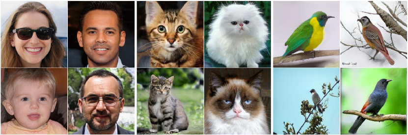
Figure 4: Visualization results of our generated images on FFHQ-256, LSUN-cat and LSUN-bird datasets, our method can generate not only high quality but also diverse images.

	FFHQ-256			LSUN-cat			LSUN-bird
	FID$\downarrow$	QS$\uparrow$	DDS$\downarrow$	FID$\downarrow$	QS$\uparrow$	DDS$\downarrow$	FID$\downarrow$	QS$\uparrow$	DDS$\downarrow$
StyleGAN	11.69	0.703	0.250	9.66	0.486	0.203	10.26	0.513	0.136
+Prior(R101)	8.79	0.724	0.199	8.25	0.526	0.162	9.04	0.530	0.109
+Prior(InV3)	7.12	0.749	0.170	7.21	0.553	0.151	8.44	0.554	0.086

Table 3: Comparison of FID, QS, and DDS metrics on three different datasets: FFHQ-256, LSUN-cat, and LSUN-bird.

	FFHQ-256			LSUN-cat			LSUN-bird
	FID$\downarrow$	QS$\uparrow$	DDS$\downarrow$	FID$\downarrow$	QS$\uparrow$	DDS$\downarrow$	FID$\downarrow$	QS$\uparrow$	DDS$\downarrow$
StyleGAN	11.69	0.703	0.250	9.66	0.486	0.203	10.26	0.513	0.136
StyleGAN +$\mathcal{L}_{Q}$	9.75	0.732	0.229	8.85	0.531	0.188	9.17	0.534	0.123
StyleGAN +RS	10.00	0.715	0.196	9.11	0.505	0.149	9.79	0.521	0.095

Table 4: Ablation study of our proposed prior with only quality loss and only resampling strategy.

4.3 Prior for Various Datasets

We also try to apply our proposed prior for various datasets, such as FFHQ-256, LSUN-cat and LSUN-bird. StyleGAN [16] recently achieve great success for high-resolution image generation. In this section, we try to combine our method with StyleGAN and evaluate the results on these datasets. We apply two different pre-trained models, ResNet101 [11] and InceptionV3 [30] to extract deep features for building the GMM model. We call them +Prior(R101) and +Prior(InV3), respectively. The quantitative results are shown in Table 3. We can observe that our approach can effectively improve the quality(QS), diversity(DDS), and the overall score(FID) over the strong baseline StyleGAN by large margins on all datasets. And the real data prior build on the feature extracted with InceptionV3 model achieves better results than ResNet101, one possible reason is that the evaluation methods are also based on InceptionV3 model. Some visualization results are shown in Figure 4.

$M$	FID$\downarrow$	QS$\uparrow$	DDS$\downarrow$
5	7.26	0.548	0.156
7	7.21	0.553	0.151
10	7.32	0.552	0.159
20	7.36	0.549	0.163
50	7.45	0.543	0.177

Table 5: PriorGAN results on LSUN-cat dataset with different number of Gaussian components $M$.

$\delta$	FID$\downarrow$	QS$\uparrow$	DDS$\downarrow$
0.03	8.31	0.509	0.191
0.07	7.82	0.529	0.201
0.10	7.66	0.550	0.195
0.15	8.11	0.578	0.220
0.2	8.29	0.586	0.227

Table 6: PriorGAN results on LSUN-cat dataset with different quality loss weight $\delta$.

$\alpha$	FID$\downarrow$	QS$\uparrow$	DDS$\downarrow$
1	8.76	0.499	0.177
3	8.35	0.506	0.162
5	8.30	0.514	0.143
7	8.08	0.521	0.149
9	8.16	0.515	0.145

Table 7: PriorGAN results on LSUN-cat dataset with different resample weight $\alpha$.

4.4 Ablation Study

To validate the effectiveness of our proposed two key methods: the quality loss and resampling strategy, we apply additional experiments on FFHQ-256, LSUN-cat, LSUN-bird dataset. The quality loss $\mathcal{L}_{Q}$ and resampling strategy are applied independently to StyleGAN. The resulting models are called StyleGAN +$\mathcal{L}_{Q}$ and StyleGAN +RS. The results are shown in Table 4. We can observe that adding the loss function $\mathcal{L}_{Q}$ mainly improve QS, which indicates the loss function $\mathcal{L}_{Q}$ mainly solve the low quality problem. Adding the resampling strategy can get a lower DDS, which indicates that the resampling strategy mainly solves the missing modes problem. This further validates the effectiveness of our proposed methods.

4.5 Hyper Parameter Analysis

In this section, we conduct experiments to investigate the sensitiveness of the number of Gaussian components $M$, quality loss weight $\delta$, and resample weight $\alpha$ in our proposed method. All the experiments are applied to the LSUN-cat dataset.

To reduce the computation cost, we apply PCA on the feature extracted from InceptionV3 model and keep 98% of the total variance by default. First, we explore how the number of Gaussian components $M$ affects the results. We set $M$ to 5,7,10,20,50 and test the results on LSUN-cat dataset, we show the results in Table 7. The results are not very sensitive to $M$ and we achieve the best performance when setting it to 7. Besides, we set $M$ to 7 and explore how quality loss weight $\delta$ and resample weight $\alpha$ affects the performance, the results are shown in Table  7, 7.

5 Conclusion

In this paper, we analyze current GANs suffer from low quality and missing modes problem. To tackle this problem, we propose a novel method which builds a GMM prior on deep feature space, by using this GMM prior, we propose quality loss to increase generated image quality and resampling strategy to enrich the diversity. Experiments have shown our method can easily insert into any GAN baseline and outperforms state-of-the-art by large margins.

Broader Impact

Our PriorGAN is a general method for image generation. From the positive aspect, many generation tasks like image-to-image translation, image editing will benefit from it. We hope our work will serve as a solid baseline and can ease future research in generative models. From the negative aspect, our method can also be applied to some image manipulation techniques, which may cause severe trust issues and security concerns in our society.

References

- [1] Jonas Adler and Sebastian Lunz. Banach wasserstein gan. In Advances in Neural Information Processing Systems, pages 6754–6763, 2018.
- [2] Martin Arjovsky, Soumith Chintala, and Léon Bottou. Wasserstein gan. arXiv preprint arXiv:1701.07875, 2017.
- [3] Jianmin Bao, Dong Chen, Fang Wen, Houqiang Li, and Gang Hua. Cvae-gan: fine-grained image generation through asymmetric training. In Proceedings of the IEEE International Conference on Computer Vision, pages 2745–2754, 2017.
- [4] Andrew Brock, Jeff Donahue, and Karen Simonyan. Large scale gan training for high fidelity natural image synthesis. arXiv preprint arXiv:1809.11096, 2018.
- [5] Jiezhang Cao, Langyuan Mo, Yifan Zhang, Kui Jia, Chunhua Shen, and Mingkui Tan. Multi-marginal wasserstein gan. In Advances in Neural Information Processing Systems, pages 1774–1784, 2019.
- [6] Arthur P Dempster, Nan M Laird, and Donald B Rubin. Maximum likelihood from incomplete data via the em algorithm. Journal of the Royal Statistical Society: Series B (Methodological), 39(1):1–22, 1977.
- [7] Jinhao Dong and Tong Lin. Margingan: Adversarial training in semi-supervised learning. In Advances in Neural Information Processing Systems, pages 10440–10449, 2019.
- [8] Ian Goodfellow, Jean Pouget-Abadie, Mehdi Mirza, Bing Xu, David Warde-Farley, Sherjil Ozair, Aaron Courville, and Yoshua Bengio. Generative adversarial nets. In Advances in neural information processing systems, pages 2672–2680, 2014.
- [9] Shuyang Gu, Jianmin Bao, Hao Yang, Dong Chen, Fang Wen, and Lu Yuan. Mask-guided portrait editing with conditional gans. In Proceedings of the IEEE Conference on Computer Vision and Pattern Recognition, pages 3436–3445, 2019.
- [10] Ishaan Gulrajani, Faruk Ahmed, Martin Arjovsky, Vincent Dumoulin, and Aaron C Courville. Improved training of wasserstein gans. In Advances in neural information processing systems, pages 5767–5777, 2017.
- [11] Kaiming He, Xiangyu Zhang, Shaoqing Ren, and Jian Sun. Deep residual learning for image recognition. In The IEEE Conference on Computer Vision and Pattern Recognition (CVPR), June 2016.
- [12] Martin Heusel, Hubert Ramsauer, Thomas Unterthiner, Bernhard Nessler, and Sepp Hochreiter. Gans trained by a two time-scale update rule converge to a local nash equilibrium. In Advances in neural information processing systems, pages 6626–6637, 2017.
- [13] Aapo Hyvärinen and Erkki Oja. Independent component analysis: algorithms and applications. Neural networks, 13(4-5):411–430, 2000.
- [14] Phillip Isola, Jun-Yan Zhu, Tinghui Zhou, and Alexei A Efros. Image-to-image translation with conditional adversarial networks. In Proceedings of the IEEE conference on computer vision and pattern recognition, pages 1125–1134, 2017.
- [15] Tero Karras, Timo Aila, Samuli Laine, and Jaakko Lehtinen. Progressive growing of gans for improved quality, stability, and variation. arXiv preprint arXiv:1710.10196, 2017.
- [16] Tero Karras, Samuli Laine, and Timo Aila. A style-based generator architecture for generative adversarial networks. In Proceedings of the IEEE Conference on Computer Vision and Pattern Recognition, pages 4401–4410, 2019.
- [17] Alex Krizhevsky, Geoffrey Hinton, et al. Learning multiple layers of features from tiny images. 2009.
- [18] Qi Mao, Hsin-Ying Lee, Hung-Yu Tseng, Siwei Ma, and Ming-Hsuan Yang. Mode seeking generative adversarial networks for diverse image synthesis. In Proceedings of the IEEE Conference on Computer Vision and Pattern Recognition, pages 1429–1437, 2019.
- [19] Xudong Mao, Qing Li, Haoran Xie, Raymond YK Lau, Zhen Wang, and Stephen Paul Smolley. Least squares generative adversarial networks. In Proceedings of the IEEE International Conference on Computer Vision, pages 2794–2802, 2017.
- [20] Takeru Miyato, Toshiki Kataoka, Masanori Koyama, and Yuichi Yoshida. Spectral normalization for generative adversarial networks. arXiv preprint arXiv:1802.05957, 2018.
- [21] KANCHARLA PARIMALA and Sumohana Channappayya. Quality aware generative adversarial networks. In Advances in Neural Information Processing Systems 32, pages 2948–2958. Curran Associates, Inc., 2019.
- [22] KANCHARLA PARIMALA and Sumohana Channappayya. Quality aware generative adversarial networks. In Advances in Neural Information Processing Systems, pages 2944–2954, 2019.
- [23] Guim Perarnau, Joost Van De Weijer, Bogdan Raducanu, and Jose M Álvarez. Invertible conditional gans for image editing. arXiv preprint arXiv:1611.06355, 2016.
- [24] Alec Radford, Luke Metz, and Soumith Chintala. Unsupervised representation learning with deep convolutional generative adversarial networks. arXiv preprint arXiv:1511.06434, 2015.
- [25] Marc’aurelio Ranzato, Volodymyr Mnih, and Geoffrey E Hinton. Generating more realistic images using gated mrf’s. In Advances in Neural Information Processing Systems, pages 2002–2010, 2010.
- [26] Eitan Richardson and Yair Weiss. On gans and gmms. In Advances in Neural Information Processing Systems, pages 5847–5858, 2018.
- [27] Ruslan Salakhutdinov and Geoffrey Hinton. Deep boltzmann machines. In Artificial intelligence and statistics, pages 448–455, 2009.
- [28] Akash Srivastava, Lazar Valkov, Chris Russell, Michael U Gutmann, and Charles Sutton. Veegan: Reducing mode collapse in gans using implicit variational learning. In Advances in Neural Information Processing Systems, pages 3308–3318, 2017.
- [29] Thad Starner and Alex Pentland. Real-time american sign language recognition from video using hidden markov models. In Motion-based recognition, pages 227–243. Springer, 1997.
- [30] Christian Szegedy, Vincent Vanhoucke, Sergey Ioffe, Jon Shlens, and Zbigniew Wojna. Rethinking the inception architecture for computer vision. In Proceedings of the IEEE conference on computer vision and pattern recognition, pages 2818–2826, 2016.
- [31] Dávid Terjék. Virtual adversarial lipschitz regularization. arXiv preprint arXiv:1907.05681, 2019.
- [32] Matthew Turk and Alex Pentland. Face recognition using eigenfaces. In Proceedings. 1991 IEEE computer society conference on computer vision and pattern recognition, pages 586–587, 1991.
- [33] Ting-Chun Wang, Ming-Yu Liu, Jun-Yan Zhu, Andrew Tao, Jan Kautz, and Bryan Catanzaro. High-resolution image synthesis and semantic manipulation with conditional gans. In Proceedings of the IEEE conference on computer vision and pattern recognition, pages 8798–8807, 2018.
- [34] David Warde-Farley and Yoshua Bengio. Improving generative adversarial networks with denoising feature matching. 2016.
- [35] Lei Xu and Michael I Jordan. On convergence properties of the em algorithm for gaussian mixtures. Neural computation, 8(1):129–151, 1996.
- [36] Jianwei Yang, Anitha Kannan, Dhruv Batra, and Devi Parikh. Lr-gan: Layered recursive generative adversarial networks for image generation. arXiv preprint arXiv:1703.01560, 2017.
- [37] Fisher Yu, Ari Seff, Yinda Zhang, Shuran Song, Thomas Funkhouser, and Jianxiong Xiao. Lsun: Construction of a large-scale image dataset using deep learning with humans in the loop. arXiv preprint arXiv:1506.03365, 2015.
- [38] Han Zhang, Ian Goodfellow, Dimitris Metaxas, and Augustus Odena. Self-attention generative adversarial networks. arXiv preprint arXiv:1805.08318, 2018.
- [39] Zhiming Zhou, Jiadong Liang, Yuxuan Song, Lantao Yu, Hongwei Wang, Weinan Zhang, Yong Yu, and Zhihua Zhang. Lipschitz generative adversarial nets. arXiv preprint arXiv:1902.05687, 2019.