Feature Extraction for Novelty Detection
in Network Traffic

Abstract.

Data representation plays a critical role in the performance of novelty detection (or “anomaly detection”) methods in machine learning. The data representation of network traffic often determines the effectiveness of these models as much as the model itself. The wide range of novel events that network operators need to detect (e.g., attacks, malware, new applications, changes in traffic demands) introduces the possibility for a broad range of possible models and data representations. In each scenario, practitioners must spend significant effort extracting and engineering features that are most predictive for that situation or application. While anomaly detection is well-studied in computer networking, much existing work develops specific models that presume a particular representation—often IPFIX/NetFlow. Yet, other representations may result in higher model accuracy, and the rise of programmable networks now makes it more practical to explore a broader range of representations. To facilitate such exploration, we develop a systematic framework, open-source toolkit, and public Python library that makes it both possible and easy to extract and generate features from network traffic and perform and end-to-end evaluation of these representations across most prevalent modern novelty detection models. We first develop and publicly release an open-source tool, an accompanying Python library (NetML), and end-to-end pipeline for novelty detection in network traffic. Second, we apply this tool to five different novelty detection problems in networking, across a range of scenarios from attack detection to novel device detection. Our findings general insights and guidelines concerning which features appear to be more appropriate for particular situations.

1. Introduction

Novelty detection (often also referred to as anomaly detection) is a common network management task: Network operators commonly need to detect and respond to a wide variety of new or unusual events, such as malicious attacks, failures, misconfigurations, changes in traffic demands, the introduction of new devices to the network, and so forth. These events can be indicative of many types of noteworthy events, including network or physical security incidents, device or infrastructure malfunctions, even behavioral changes in the users of the devices that might be indicative of abnormal human conditions or behaviors.

The goal of detecting such new, unseen events falls under the general category of novelty detection (also known as anomaly detection) problems in machine learning, for which there are many possible procedures, including Gaussian mixture models (GMM), one-class support vector machines (OCSVM), kernel density estimation (KDE), and others. The effectiveness of any of these procedures—and, in fact, for any machine learning approach—depends fundamentally on how the data are represented as input features to the model. Often the choice of features and how they are represented—the process of feature extraction—determines the accuracy and effectiveness of the approach than the choice of model.

Representations of network traffic that are most effective for novelty detection are typically a priori unclear. Representation choices typically involve various statistics concerning traffic volumes, packet sampling rates, and aggregation intervals. Yet, which of these transformations retain predictive information is typically initially unknown. While novelty detection is a problem for many problems in networking, and for network traffic in general, the problem is particularly challenging for Internet of Things (IoT) traffic, given the wide range of device types, vendors, traffic patterns, interaction modes, and failure scenarios across devices. One example challenge is choosing the granularity on which to aggregate a feature: For instance, if we decide to measure and represent the number of packets per second as a feature, then changes in traffic patterns at the millisecond level might go undetected; on the other hand, recording at this granularity creates higher dimensional observations introducing high-dimensional data that creates challenges with both scale and accuracy. (The so-called curse of dimensionality in machine learning is the observed fact that the higher the dimension of the input, the harder it is to achieve good accuracy; in particular, we might then require an amount of training data exponential as a function of dimension.)

This paper explores how the process of feature extraction from raw network traffic affects the accuracy of a variety of novelty detection methods for a range of novelty detection problems in network traffic. To facilitate the reproducibility of these results and further research on novelty detection from network traffic, we have released our feature extraction methods as an open-source library and a publicly available Python package on PyPi. We aim to explore how different data representations for network traffic affect novelty detection rates, across (1) different types of novelty detection problems; (2) different types and classes of network devices; (3) a range of unsupervised machine learning models. We focus on identifying novel network flows, a common, intuitive unit of identification that, at a high-level, represents a single exchange of data between two network endpoints. The ability to identify a novel flow lends itself to detecting other types of novelty; for example, a device that generates novel traffic flows may itself be considered novel.

There are many possible ways to represent raw traffic traces (i.e., packets) as inputs. The data itself can be aggregated on various time windows, elided, transformed into different bases, sampled, and so forth. We focus on representations of network traffic data that do not incorporate semantics from the header itself, such as IP addresses, port numbers, sequence numbers, or other specific values in the packet headers themselves. Representations that are agnostic to specific values in the headers ensures that the resulting models are trained to recognize novel behavior regardless of the specific source, destination, application, or location in the network. In contrast to past work in this area, which has typically focused on a single problem in novelty detection using a single dataset and a chosen procedure, our focus is on studying the applicability of representation, we aim for generality and reproducibility of results across a range of problems, studying the applicability of different representations across a range of problems.

When evaluating different feature representations across models and problem domains, we design methods and metrics that result in comparisons that are as fair as possible. We report the area under the ROC curve (AUC) for each approach, scenario, and dataset. Because machine learning procedures are very sensitive to hyperparameter choices (e.g., bandwidth choice in OCSVMs, or the number of dimensions in PCA), we consider both the best possible choices of such hyperparameters (which unfortunately are hard to find in practice without labeled data), and default choices that might be made in practice based on rules-of-thumb. To ensure an apples-to-apples comparison across procedures, we ensure that all data representations result in feature vectors of a similar order in dimension, in the range of 10 to 30 dimensions. Our goal is not to identify the best outlier detection model but rather to demonstrate that certain feature representations are effective across models. The public, open-source library that we have released makes it possible to transform raw packet captures into the representations we explore in this paper and explore the accuracy of outlier detection across many families of models.

Our exploration of different novelty detection procedures across a range of networking problems yields the following findings:

• No single data representation works best across all devices and models. The lack of a singe best representation underscores the importance of exploring a wide range of possible features and representations, which we have made possible through the release of an open-source toolkit and Python library.

• Incorporating metadata such as packet size and header information (e.g., IP TTL, TCP flags) significantly improves the accuracy of novelty detection, across a variety of models and outlier detection techniques. This result has significant implications on past work in the Internet measurement and security areas, which have focused predominantly on representations such as IPFIX (e.g., NetFlow), which do not incorporate these features.

• Frequency domain representations often have little effect on model accuracy. Contrary to expectations, performing a Fourier transform on the raw network packet traces generally has minimal effect on model accuracy, regardless of the representation of the data in the time domain.

These results hold generally across all families of models we explore, for a wide range of anomaly detection models, from physical device anomalies to security events. These results represent a promising step forward for anomaly detection, as they demonstrate that packet header values—which are simple to extract and visible even when traffic is encrypted—can be sufficient for anomaly detection, independent of model, subject to the appropriate transformations on their representation. To make these transformations possible, to facilitate the reproducibility of our results as well as follow-on work that can make use of the packet transformation capabilities we have developed and evaluated in this work, we have published our source code as an open-source software library (itod-code, ).

The rest of the paper is organized as follows. Section 2 discusses related work, and Section 3 outlines the common ways of representing network traffic flows in the literature. It is difficult to be completely exhaustive, yet we focus on the most established approaches for representing traffic data both in general network anomaly detection and in the growing literature on novelty detection for IoT, comparing tuning and configuration and tuning decisions that might be made in practice. Section 4 outlines the machine learning models and performance metrics that we use for our comparative analysis, the metrics that we use to evaluate these models. and the setup of our experiments, how we selected hyperparameters for various novelty detection models, and the datasets that we used in our evaluation and how we processed those datasets. Section 7 describes the results from our experiments, and Section 8 concludes with a summary and directions for future work.

2. Related Work

Novelty detection in computer networking is a well-explored topic. Past research has explored relatively standard techniques, such as Principal Component Analysis (PCA), for anomaly detection in network traffic. Clustering approaches, including PCA-based clustering approaches (e.g., spectral clustering) has also been applied to network traffic to detect anomalous behavior. In contrast, relatively less attention has been paid to a broader range of more modern anomaly detection models that we explore in this paper—many of which outperform PCA. Previous work has also applied various techniques towards novelty detection using a broad range of data representations, without comparing the (potentially significant) effect that data representation can have on model accuracy. We briefly survey related work in both unsupervised learning methods for novelty detection in networking, as well as various data representations that past research has used for novelty detection.

Principal Component Analysis.

Previous work has focused on the use of unsupervised methods for novelty detection—sometimes also referred to as “anomaly detection”. A significant amount of work on anomaly detection in network traffic has focused on Principal Component Analysis (PCA). PCA has been used detect anomalous traffic flows in network backbones (lakhina2005mining, ; lakhina2004diagnosing, ; lakhina2004structural, ). Subsequent work observed that the effectiveness of PCA for network anomaly detection has a significant dependence on how network traffic data is represented (ringberg2007sensitivity, ). This work found that PCA is sensitive to various aspects of data representation, including the level of aggregation that is performed in the original traffic traces. This work and and others also demonstrated that PCA-based anomaly detection is not robust to noise (rubinstein2009stealthy, ). More recently, PCA has been applied to anomaly detection for in IoT network traffic (hoang2018pca, ).

Despite the significant attention devoted to PCA for anomaly detection, relatively little attention has been paid to the much broader family of anomaly detection that we study in this paper, including models that can learn non-linear decision boundaries for detecting novel activity (e.g., one-class SVM, auto-encoder) as we explore in this paper. Furthermore, as previously discussed, the representation of the traffic data is often at least as important as the choice of model; Ringberg et al. first noted the sensitivities of PCA to data representation in 2007 (ringberg2007sensitivity, ). Despite the importance of data representation on detection accuracy, there has been little study of this problem. To our knowledge, our work is the first to explore a wide range of possibilities for representing network traffic, for a large collection of datasets and models.

Clustering Techniques.

Clustering techniques have been used to detect certain types of malicious network activity such as botnets (gu2008botminer, ) and web-based malware (perdisci2010behavioral, ). These works apply hierarchical clustering techniques to identify groups of hosts that are behaving in a similar fashion, thereby indicating potential botnet membership. Other clustering techniques, such as spectral clustering, have been applied to email traffic to detect spammers (ramachandran2007filtering, ). These methods are generally specific to the detection of botnet behavior, which tends to cluster well; additionally, this past research uses a variety of traces (e.g., IPFIX/NetFlow, HTTP traces, email logs). Our work focuses instead on novelty detection in raw packet traces, across many models and novelty detection problems.

Metric Learning and Representation Learning.

The importance of data representation for model accuracy has fostered many subfields such as metric learning and representation learning, which aim to automatically find the right representation to be coupled with given procedures, so far with mixed results. These techniques have achieved much success in application areas such as computer vision and speech processing, yet no such automated approaches exist in the fledgling application area of novelty detection for network traffic, particularly for networked IoT devices. A main aim of this work is to bring attention to the importance of data representation, and identify representations that work well in general while meeting practical requirements for succinct, efficient representations.

Data Representations for Anomaly Detection.

Previous work has explored the use of various subsets of network traffic features for detecting anomalies and security incidents in network traffic. Lakshari et al. used flow direction, interarrival time, and packet sizes as features (lashkari2018toward, ); Mukar et al. used packet inter-arrival time (kumar2018novel, ), and Mirsky et al. used flow statistics over fixed time intervals, or windows, as feautres (mirsky2018kitsune, ). Other researchers have explored various combinations of these features for IoT anomaly detection (aljawarneh2018garuda, ; doshi2018machine, ; meidan2018n, ; bhatia2019unsupervised, ; thamilarasu2019towards, ), specifically, as well as for detection of distributed denial of service (DDoS) attacks (fouladi2016frequency, ; lima2019smart, ). Table 1 summarizes this past work, and various data representations that each has used in developing novelty detection models. All of this past research differs significantly from our work, in that each work typically applies one representation and model to a specific problem. In contrast, our work attempts to explore all of these representations across a wide range of models, evaluating how well specific representations work for different types of novelty detection problems. To our knowledge, our work is the first to take such a holistic approach to novelty detection in network traffic, and the first to explore a holistic approach to a wide range of settings and scenarios in IoT.

3. Representing Network Traffic

Machine learning procedures require for the most part, feature vectors of the same dimension, i.e., every flow has to be represented as a vector of a fixed number of carefully chosen features, specifically information extracted from the flow.

Flows.

We consider various feature representations of forward flows, where a forward flow aggregates all packets, with a same five-tuple identifier, sent from a device being monitored to another device or server. The five-tuple identifier consists of source IP address, source port, destination IP address, destination port, and protocol. We consider the following representations of flows:

Reference	Duration	IAT	SIZE	FFT	SAMP-NUM	SAMP-SIZE
Network Intrusion Detection
Lakshari et al. (lashkari2018toward, )	✓	✓	✓	✗	✗	✗
Mukar et al. (kumar2018novel, )	✗	✓	✗	✗	✗	✗
Mirsky et al. (mirsky2018kitsune, )	✗	✗	✗	✗	✓	✓
IoT Anomaly Detection
Al Jawarneh et al.(aljawarneh2018garuda, )	✓	✗	✓	✗	✗	✗
Doshi et al. (doshi2018machine, )	✗	✓	✓	✗	✗	✗
Meidan et al. (meidan2018n, )	✗	✓	✗	✗	✓	✓
Bhatia et al. (bhatia2019unsupervised, )	✗	✗	✓	✗	✓	✗
Thamilarasu et al. (thamilarasu2019towards, )	✗	✗	✓	✗	✗	✗
DDoS Detection
Fouladi et al. (fouladi2016frequency, )	✗	✗	✗	✓	✗	✗
Lima et al. (lima2019smart, )	✗	✗	✓	✗	✗	✗

Table 1. Commonly used data representations for novelty detection.

• STATS: A flow is represented as a set of statistical quantities. We choose ten of the most common such statistics in the literature (see i.e, (Moore2005, )): flow duration, number of packets sent per second, number of bytes per second, and various statistics on packet sizes within each flow: mean, standard deviation, inter-quartile range, minimum, and maximum.

• SIZES: A flow is represented as a timeseries of packet sizes in bytes, with one sample per packet.

• IAT: A flow is represented as a timeseries of inter-arrival times between packets, i.e., elapsed time in seconds between any two packets in the flow.

• SAMP-NUM: A flow is partitioned into small intervals of equal length $\delta t$, and the number of packets in each interval is recorded; thus a flow is represented as a timeseries of packet counts in small time intervals, with one sample per time interval. Here, $\delta t$ might be viewed as a choice of sampling rate for the timeseries, hence the nomenclature.

• SAMP-SIZE: A flow is partitioned into time intervals of equal length $\delta t$, and the total packet size (i.e., byte count) in each interval is recorded; thus, a flow is represented as a timeseries of byte counts in small time intervals, with one sample per time interval.

Any of these timeseries representations might be given in time or Fourier domain, in which case we append FFT to the representation name, i.e., IAT-FFT, SAMP-NUM-FFT, and SAMP-SIZE-FFT.

In all cases, we avoid any representations that rely on or encode specific values of packet headers, such as the value of a source or destination IP address or port number, the value of a protocol (e.g., TCP, UDP), and so forth, to avoid developing models that would define normal behavior as specific to a particular network attachment point (e.g., IP address or port). We avoid training models based on these values for several reasons. Most importantly, training a model based on IP address values would define anomaly simply as any deviation in network destinations from those in the trained model. A model trained on traffic traces collected in one part of the network would not be able to perform general novelty detection when applied or deployed on other parts of the network. The model would also fail to detect novel behaviors from the same IP addresses over time—as would be the case if a device were compromised or simply changed its behavior as result of changes in the environment or how users interacted with the device over time. For similar reasons, we avoid relying on port numbers. On the one hand, a significant amount of traffic—both normal and novel—traverses common ports (e.g., port 443, or HTTPS); on the other hand, client traffic originates from ports that change (e.g., increment) all of the time, and thus defining normal traffic based on client ports would result in a significant amount of false positives simply based on the normal behavior of clients originating connections from different ports over time.

When applying different machine learning models for novelty detection, we must ensure that all of the above representations result in feature vectors of the same dimension for any given device being monitored. This is automatically the case for STATS, but not for the other representations, in light of variations in flow durations and lengths (number of packets) for a given device. To ensure that each sample has the same dimension, we select a fixed time duration for all flows corresponding to the 90th percentile of all flow lengths or durations for a device. We use this duration so as to capture the typical behavior of most device instances of a particular type. Any definition of typicality may be appropriate here, depending on the desired compactness and complexity of the corresponding representation. Using the 90th percentile of all flow durations results in a comparable number of dimensions (typically 10–30) for most of the devices that we consider in this study.

4. Models and Metrics

We describe the novelty detection procedures that we evaluate in our study, as well as the performance metrics that we use to compare each of these procedures. We then describe the datasets we use to evaluate each novelty detection method, including how we process each of these datasets and select parameters for each corresponding feature representation. Finally, we describe the process by which we choose hyperparameters for each of the novelty detection procedures that we evaluate in this study.

4.1. Novelty Detection Models

We consider popular novelty detection procedures from machine learning and statistics, approaches based on six models:

• One-Class Support Vector Machines (OCSVM),

• Isolation Forests (IF),

• Auto Encoders (AE)

• Kernel Density Estimation (KDE)

• Gaussian Mixture Models (GMM), and

• Principal Component Analysis (PCA).

Important common aspects of all such detection procedures are as follows:

1. Data representation as features. Novelty detection procedures invariably require data—network flows—represented as a vector $X\in\mathbb{R}^{d}$ of $d$ predictive features. While many procedures operate directly on that feature representation (e.g., IF, KDE, GMM), others (e.g., OCSVM, PCA, AE) remap vectors $X$ into refined representations where certain patterns—clusters of similar network activities—might be more evident.

2. Training and testing. Models are trained in a first phase using $n$ training data points $\{X_{i}\}_{i=1}^{n}$ – i.e., $n$ copies $X_{i}$ of typical values of normal features $X$ (e.g., each $X_{i}$ representing a normal traffic flow), from which they produce a scoring function $S(X)$; high scores $S(X)$ are expected to be typical of normal observations such as the training data points $X_{i}$, while low-scores would be indicative of the query $X$ being an outlier (novelty). Subsequently, in the so-called testing phase (or deployment phase), a threshold $t$ might be chosen so that any query $X$ is flagged as novelty whenever $S(X)<t$.

In practical settings, the right choice of threshold can be difficult since the available training data is assumed to be all normal, making it difficult to assess false negative rates. Instead, one might choose a threshold based on the false positive rates the application can tolerate, which can be estimated for each choice of $t$ based on the normal data (i.e., data known to not have positive label). Related issues are discussed in Section 4.2 on performance metrics.

Normality scores in ML:

In KDE or GMM, the training data is used to estimate the density function $f$ of the data in $\mathbb{R}^{d}$ (that is their spatial distribution), where by definition $f(x)$ is low in those regions of space that have little data. This density would then serve as a scoring function $S(X)\doteq f(X)$. IF works similarly by first partitioning the space $\mathbb{R}^{d}$ into ensembles of high and low density regions, and flagging any query $X$ as a novelty if it lies in a low density region.

On the other hand, PCA and AE work by identifying a lower-dimensional space ${\mathcal{}X}$ embedded in the representation space $\mathbb{R}^{d}$ on which most of the training datapoints $X_{i}$ appear to lie. In PCA $\mathcal{}X$ is a linear space, while in AE it can be highly nonlinear (using nonlinear activation functions in a neural network). The score $S(X)$ then denotes how close $X$ is to $\mathcal{}X$ with lowest scores for points farthest from $\mathcal{}X$.

OCSVM stands farther apart as it proceeds by first remapping all $X_{i}$’s – through a transformation $\Phi(X_{i})$ into a higher dimensional feature space $\mathcal{}H$ (possibly of infinite dimension) and then essentially identifying regions of high density in $\mathcal{}H$, typically by fitting a hyperplane separating the embedded normal data from the origin $0\in\mathcal{}H$. The underlying assumption is that patterns might be more visible in $\mathcal{}H$, for instance, all $\Phi(X_{i})$ might cluster together into a normal region (typically a half space in $\mathcal{}H$, or sometimes an enclosing ball; the score $S(X)$ is then lower for queries $X$ that map as $\Phi(X)$ outside the normal region of $\mathcal{}H$.

Although we analyze all the above described procedures, we restrict attention to a few representative such ML procedures in the main body of the paper (see Section 7), while all additional substantiating results can be found in the appendix.

4.2. Performance Metrics

Area Under the Curve (AUC):

As explained above, detection procedures flag a new query $X$ as novel if it scores below a certain threshold $t$ (i.e., if $S(X)<t$). Now notice a tension: the higher the threshold $t$, the more likely it is that all novel $X$ are correctly detected, but unfortunately, the more likely it is also that normal datapoints are flagged as novel (a false alarm). Thus, the best performing approaches—combination of data representation and choice of detection procedure—are those that alleviate this tension, performing accurate detection while minimizing false positives.

Such tradeoffs are well captured by a Receiver Operating Characteristic (ROC) curve, which plots the detection rate against the false alarm rate as $t$ is varied from small to large; a large area under the curve (AUC) indicates that good tradeoffs are possible under the given detection approach. We therefore adopt AUC as a sensible measure of performance.

Sensitivity to Hyperparameters:

All detection procedures come with hyperparameters, i.e., configuration choices that can greatly affect performance. Important hyperparameters are e.g., bandwidth in KDE or OSCVM, number of partitions in IF, number of components in GMM, embedding dimension in PCA and AE. We therefore have to carefully pick such parameters in practice, although the right approach remains unclear, especially in unsupervised learning problems such as novelty detection where we typically do not have a labeled validation set to evaluate choices.

Since hyperparameter tuning in unsupervised learning remains the subject of ongoing research in Machine Learning and Statistics, we decided to present results for the best choices of parameters, picked as those choices that result in the best performance on a separate validation set, and used to report results on an independent test set. The tuning parameters for each method are described in Section 6.2 below, while Appendix A.2 gives data sizes (with validation kept around 1/4 test sizes).

More configuration details such as range or parameters are given in Section 6.2. Other configuration choices based on common rule-of-thumbs are covered in more detail in the appendix along with relevant results.

5. NetML: A Novelty Detection Library for Network Traffic

We have designed, implemented, and released a public, open-source Python library, netml, that takes network packet traces as input, transforms these packet traces into the various data representations as outlined in Section 4. We have released the open-source code for the library and packaged the library on PyPi for easy installation.

⬇

1from netml.pparser.parser import PCAP

2from netml.utils.tool import dump_data

3

4pcap = PCAP(

5 ’data.pcap’,

6 flow_ptks_thres=2,

7 random_state=42,

8 verbose=10,

9)

10

11# extract flows from pcap

12pcap.pcap2flows(q_interval=0.9)

13

14# label each flow (optional)

15pcap.label_flows(label_file=’labels.csv’)

16

17# extract features from each flow via IAT

18pcap.flow2features(’IAT’, fft=False, header=False)

19

20# dump data to disk

21dump_data((pcap.features, pcap.labels),

22 out_file=’IAT-features.dat’)

Listing 1: From packet capture to features.

The netml library is written in Python and contains two sub-modules: (1) a pcap parser to produce flows using Scapy/dpkt; (2) a novelty detection module that applies the novelty detection algorithms we outlined in Section 4 to the resulting flow-based features. The netml functionality can be incorporated as a Python library or invoked directly from the command line. The entire library consists of approximately 11,000 lines of Python, with the packet parsing module comprising approximately 3,500 lines of Python, the implementations of various novelty detection modules comprising another 3,000 lines, another 3,000 lines in support of the netml command-line utility, and the rest of the code in support of various utilities (e.g., testing).

Listing 1 shows the basic functions to extract features from traffic flows. Line 12 extracts flow from the packet capture and Line 15 labels time intervals in the flow according to whether those are normal or anomalous. The flows2features function at line 18 extracts features from the flows in the pcap according to the specified parameters. The library currently supports all of the representations outlined in Section 3.

⬇

1from netml.ndm.model import MODEL

2from netml.ndm.ocsvm import OCSVM

3from netml.utils.tool import dump_data, load_data

4

5# load data

6(features, labels) = load_data(’IAT-features.dat’)

7

8# split train and test sets

9(

10 features_train,

11 features_test,

12 labels_train,

13 labels_test,

14) = train_test_split(features, labels,

15 test_size=0.2)

16

17# create detection model

18ocsvm = OCSVM(kernel=’rbf’, nu=0.5)

19ocsvm.name = ’OCSVM’

20ndm = MODEL(ocsvm, score_metric=’auc’)

21

22# train the model from the train set

23ndm.train(features_train)

24

25# evaluate the trained model

26ndm.test(features_test, labels_test)

Listing 2: Training and testing models.

Listing 2 shows an example of how the library can be used to train the model. As shown in the figure, model training and applications of the model can be performed using function calls that are analogous to those in the familiar scikit-learn API. Line 18 instantiates a particular novelty detection model (in this case, OCSVM with a radial basis function kernel), and Line 20 creates the model itself which can then be invoked with familiar train and test functions. While it is not shown in the figure, the module also records both accuracy and performance statistics that can then be written to a data structure or to persistent storage.

6. Experiment Setup

We now describe the data that we used to evaluate the collection of novelty detection algorithms and representations described in the previous section.

6.1. Data Collection and Preprocessing

We consider a combination of publicly available traffic traces and traces collected on private consumer IoT devices. We aim to evaluate representative set of devices, from multi-purpose devices such as laptop PCs, and Google Home, to less complex electronics and appliances such as smart cameras and TVs. Furthermore we aim at a representative set of novelties, from benign novelties (new activity, or a new device type), to novelties due to malicious activities (DDoS attack). Table 3 describes these datasets, and types of novelty being detected.

Detector	Dataset	[c]STATS	[c]SIZE	[c]IAT	[c]SAMP- NUM
OCSVM	UNB(PC1)	0.48	0.77	0.81	0.76
	UNB(PC4)	0.55	0.73	0.86	0.75
	CTU	0.64	0.77	0.76	0.91
	MAWI	0.88	0.47	0.45	0.59
	TV&RT	1.00	1.00	0.96	0.93
	SFrig	0.98	0.89	0.82	0.96
	BSTch	0.95	0.98	0.97	0.95
IF	UNB(PC1)	0.49	0.52	0.63	0.77
	UNB(PC4)	0.60	0.47	0.70	0.81
	CTU	0.78	0.79	0.86	0.89
	MAWI	0.86	0.69	0.42	0.62
	TV&RT	0.95	0.98	0.90	0.75
	SFrig	0.96	0.95	0.59	0.94
	BSTch	0.95	0.98	0.94	0.98
AE	UNB(PC1)	0.68	0.63	0.70	0.83
	UNB(PC4)	0.79	0.68	0.71	0.84
	CTU	0.49	0.83	0.93	0.91
	MAWI	0.49	0.62	0.46	0.60
	TV&RT	1.00	1.00	0.97	0.85
	SFrig	0.91	0.92	0.73	0.97
	BSTch	0.96	0.94	0.97	0.97
KDE	UNB(PC1)	0.31	0.77	0.83	0.72
	UNB(PC4)	0.52	0.71	0.86	0.75
	CTU	0.76	0.83	0.77	0.92
	MAWI	0.86	0.55	0.47	0.59
	TV&RT	1.00	1.00	0.97	0.89
	SFrig	0.97	0.90	0.80	0.95
	BSTch	0.94	0.98	0.95	0.95
GMM	UNB(PC1)	0.56	0.61	0.75	0.80
	UNB(PC4)	0.87	0.71	0.65	0.81
	CTU	0.69	0.70	0.90	0.90
	MAWI	0.87	0.67	0.49	0.63
	TV&RT	1.00	1.00	0.98	0.93
	SFrig	0.98	0.97	0.88	0.96
	BSTch	0.99	0.98	0.95	0.97
PCA	UNB(PC1)	0.74	0.27	0.41	0.77
	UNB(PC4)	0.72	0.60	0.74	0.75
	CTU	0.81	0.74	0.75	0.89
	MAWI	0.70	0.45	0.40	0.59
	TV&RT	0.99	1.00	0.97	0.65
	SFrig	0.80	0.91	0.71	0.95
	BSTch	0.97	0.08	0.92	0.95

Table 2. AUCs for 6 ML approaches on basic feature representations.

Reference	Device	Description	Novelty
[c]UNB IDS (cicids2017, ) (5 datasets)	Five PCs (noted as PC1, PC2, PC3, PC4, and PC5, respectively)	Normal and DDoS attack traces from personal computers (PC), which are chosen from Monday trace and Friday trace.	DDoS attack
[c]CTU IoT (ctu2019iot, ) (1 dataset)	Two Raspberry Pis	Bitcoin-Mining and Botnet traffic traces generated by two Raspberry Pis; we aim to distinguish the two devices by their attack traces (i.e., Mirai and CoinMiner); hence we use one generated CoinMiner as normal, the other generated Mirai as novel.	Novel (infected) device
[c]MAWI (mawi2019normal, ) (1 dataset)	Two PCs	Normal traffic generated by two PCs, which are collected on Dec. 07, 2019; we use one PC (whose IP address is 202.171.168.50) as normal, the other (whose IP address is 202.4.27.109) as novel.	Novel (normal) device
[c]Lab IoT (5 datasets)	A smart TV and a wireless router (noted as TV&RT)	Data is generated by a smart TV and a wireless router in a private lab environment. We collect two kinds of normal traffic generated by a smart TV (whose IP address is 10.42.0.119) and a router (whose IP address is 10.42.0.1). the router traffic is labeled as normal, and the smart TV traffic is labeled as novel.	Novel (normal) device
	Google home (GHom), Samsung camera (SCam), Samsung fridge (SFrig), and Bose soundtouch (BSTch)	Data traces are generated by IoT devices in a private lab environment. Four smart-home devices, each with two types of traffic traces labeled as normal when there is no human interaction, and novel when being operated by a human.	Novel activity

Table 3. Datasets.

Obtaining flows:

We parse upstream flows from datasets in Table 3 using Scapy (scapy, ). Given that certain devices can have arbitrarily long flows, we truncate each flow from a given dataset to have duration at most that of the 90th upper-percentile of flow durations in the dataset. Henceforth, a flow refers to these choices of flows involving truncation.

Selecting feature representation dimension:

Each flow is then represented using any of the feature-representation choices described in Section 3. Here, we have to ensure that, given a representation choice, e.g., IAT, all flows result in vectors of the same dimension $d$ for each dataset. We apply a similar approach to enforce such fixed dimension $d$, as outlined below. For a fixed dataset, let $d_{0}$ denote the 90th upper-percentile of number of packets per flow.

• STATS: automatically results in vectors of the same dimension $d$, equal to the number of statistics (on packet size) computed on a flow.

• IAT, or SIZE: dimension is fixed to $d=d_{0}-1$ for IAT, and $d=d_{0}$ for size; namely, for long flows, we truncate the number of packets in a flow to the first $d_{0}$; for short flows where the number of packets is less than $d_{0}$, we append $0$’s to the IAT representation to arrive at $d$ features.

• IAT + SIZE: just concatenates IAT and SIZE representations to dimension $d=2d_{0}-1$.

• SAMP-NUM or SAMP-SIZE: dimension is fixed to $d=d_{0}-1$ as in the case of IAT. Now we pick a fixed window size $\delta t$, and each flow is divided into up to $d$ windows of length $\delta t$; for flows of short duration, where $\delta t$ is large with respect to duration, we simply append $0$’s.

  Choice of $\delta t$: we start with candidate choices $\Delta\doteq\{t_{f}/d\}$, over durations $t_{f}$ of flows $f$ in a given dataset. We then consider 10 choices of $\delta_{t}$ in $\Delta$, each choice an $i$-th quantile of values in $\Delta$, for each $i\in\{10,20,30,40,50,60,70,80,90,95\}$. Thus, each such choice of $\delta t$ yields one (SAMP-NUM or SAMP-SIZE) representation for all flows; since we do not know which such representation (i.e. choice of $\delta t$) is best a priori we report the best AUC resulting out of all 10 choices of $\delta t$.

Each of the above representations, besides STATS, can then be viewed as fixed length time series, and therefore admit a Fourier domain representation; the corresponding Fourier representation is then set to the same dimension $d$, i.e., we retain as many Fourier components as the original time series.

The resulting representation dimensions for each dataset are reported in Table A.1 in the appendix.

6.2. Hyperparameter Settings

All detection procedures are implemented in the scikit-learn Python package. We now describe configuration choices, both for the best hyperparameter choice (Optimal)—picked using validation data (1/4 test set sizes) as described in Section 4.2 and (exact sizes in Appendix A.2)—and a rule-of-thumbs choice (Default).

• One-Class SVM (OCSVM) (scholkopf2000support, ) (implemented by (zhao2019pyod, )). We choose a Gaussian kernel of the form $K(x,x^{\prime})\propto\exp(-\|x-x^{\prime}\|^{2}/2\sigma^{2})$, and pick $\sigma$ as follows. We consider the quantiles $[0.1,0.2,\ldots,0.9]\cup\{0.95\}$ on increasing distances between pairs of points in the training sample.
  Optimal: The parameter $\sigma$ is then picked as that quantile which yields the best AUC.
  Default: $\sigma$ is picked as the 0.3 quantile of inter-point distances.

• Isolation Forest (IF) (liu2012isolation, ) (implemented by (zhao2019pyod, )). We pick the number $k$ of trees in the range 30 to 300 with increments of 10.
  Optimal: $k$ is chosen as the value in the range maximizing AUC.
  Default: $k$ is 100, which is the same as the default value in pyod.

• AutoEncoder (AE) (zhou2017anomaly, ) (from PyTorch (NEURIPS2019_9015, ) using LeakyRelu for activation functions). For $X\in\mathbb{R}^{d}$, we use the following architecture with 5 layers, determined by a tuning parameter dim: one input layer of size $d$ (number of neurons), followed by a hidden layer of size $\text{h-dim}\doteq\text{min}\{(d-1),\lceil 2\cdot\text{dim}\rceil\}$, a latent layer of size dim, a subsequent hidden layer of size h-dim, and finally an output layer of size $d$. We pick dim in a range $\{\lceil 1+i\cdot(d-2)/9\rceil\}_{i=0}^{9}$ of (up to 10) values (approximately evenly spaced) between $1$ and $d-1$.
  Optimal: dim is chosen as the value in the range maximizing AUC.
  Default: $\dim$ is $\lceil d/2\rceil$.

• Kernel Density Estimation (KDE) (latecki2007outlier, ; scott2005multidimensional, ). We use a Gaussian kernel, of the same form as OCSVM above, and pick the bandwidth $\sigma$ exactly the same way for both Optimal and Default.

• Gaussian Mixture Model (GMM) (Bishop2006Pattern, ). We choose the number of Gaussian components $k$ on a range $[1,2,5,10,15,$
  $20,25,30,35,40]$.
  Optimal: $k$ is chosen as the value in the range maximizing AUC.
  Default: $k$ is obtained as the number of high-density regions (or modes) in the training data, as obtained by the quickshift++ procedure of (jiang2018quickshift++, ).

• Principal Component Analysis (PCA) (aggarwal2015outlier, ). For $X\in\mathbb{R}^{d}$, i.e., having $d$ features, we pick the projection dimension dim in a range. We pick dim in a range $\{\lceil 1+i\cdot(d-2)/9\rceil\}_{i=0}^{9}$ of (up to 10) values (approximately evenly spaced) between $1$ and $d-1$.
  Optimal: dim is chosen as the value in the range maximizing AUC.
  Default: dim is estimated by maximum likelihood (MLE) in scikit-learn.

7. Results

In this section, we explore how data representation affects the performance of different novelty detection algorithms. After presenting baseline model accuracy across a range of models for a variety of novelty detection problems, we investigate the effects of various feature representations on model accuracy. We first then investigate whether and how packet sizes and packet header information ultimately affect novelty detection, for different types of novelty, across detection approaches. We then explore the effect of Fourier domain representations.

7.1. Baseline Model Accuracy

In order to understand how different data representations affect model accuracy, we first need to understand baseline accuracy for each model, scenario, and a baseline set of features. Because we are interested in the relative effects of additional features and transformations, including packet sizes, headers, and Fourier representations, we first present baseline levels of accuracy across models without these features. Table 2 gives baselines for comparisons. We are interested in the difference in AUC due to the presence or absence of particular feature types with respect to a set of basic feature representations, namely STATS, SIZE, IAT, SUMP-NUM, and SAMP-SIZE.

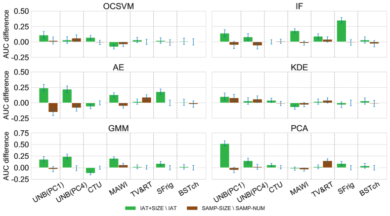
Figure 1. Differences in AUC due to including vs. excluding packet size information.

Table 2 also includes IAT+SIZE as a baseline for future comparisons). We will see that across ML models, the effect of (1) packet size information, and (2) packet header information tend to be significant overall. (3) Fourier domain representations have little advantage over raw time series (despite being generally thought of as a better way to capture important trends in timeseries) (oppenheim1999discrete, ). We focus on the most popular ML approaches disxcussed so far (OCSVM, IF, AE, KDE, PA, GMM) in the main text, under OPT tuning, while results under Default tuning, and omitted datasets are given in the appendix. The choices of procedures is meant to be representative of each major family of approach as described in Section 4.

Statistical significance.

Throughout this section, we often display error bars of length $1/\sqrt{n}$ ($n$ denoting test sample sizes as given in Table A.2), which is a ballpark for standard deviation in AUC computed on a test sample of size $n$. Training data sizes are for the most part around 5000 (see again Table A.2) besides for a few cases where they are smaller to allow large enough test size $n$ (at least a few hundred points to ensure statistical significance).

7.2. Effects of Data Representations

Given an understanding of baseline performance, we now explore the effects of various representations of network traffic on model accuracy across the range of novelty detection models and scenarios we described earlier.

7.2.1. Packet Size Information

Table 2 shows that packet size information immediately appears to be important based on the often higher AUCs achieved under STATS (which primarily compiles statistics on packet sizes in a flow) and SIZE (time series of packet sizes) to those achieved under basic representations such as IAT and SAMP-NUM (devoid of packet size information). This is most evident, e.g., under for the MAWI and SFrig datasets.

As it turns out, adding packet size information to IAT or SAMP-NUM representations improves on such representations alone. Namely, in the case of IAT, size information is added in by concatenating IAT and SIZE vectors, which we denote IAT+SIZE. For SAMP-NUM, which is a time-series of number of packets in small fixed time intervals $\delta t$, size information is integrated in by instead compiling total packet size in fixed time intervals $\delta t$.

Figure 1 presents the differences in AUC obtained using packet size information, minus those obtained on corresponding representations without size information. We observe significant positive differences for the features IAT+SIZE, across ML procedures on most datasets—which we recall, correspond to a range of novelty detection problems, whether malicious attacks, or novel devices or activity. Moreover, in most cases where size information does not yield improvements, it nonetheless does not hurt performance (changes are under the significance level shown by error bars), except in the case of dataset UNB(PC1) under SAMP when employing AE. This is however a case where packet size information remains useful with respect to IAT, just not with respect to sampling-based features SAMP. As such, it appears that for the sampling based features SAMP-SIZE and SAMP-NUM, number of packets or packet sizes in fixed time intervals are equally predictive in general. One reason for this observed effect is likely because packet sizes are predictable and are often even uniform in size, particularly for long-running and high-volume flows, where packet size is limited by the maximum transmission unit (MTU).

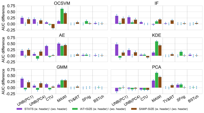
Figure 2. Differences in AUC due to including vs. excluding packet header information.

In general, the inclusion of packet sizes for novelty detection makes sense, as the packet size can provide some indication about the nature of the underlying activity. For example, for the case of the UNB dataset, attack traffic may be unique in size relative to other types of activities. In the case of the private IoT datasets (TV&RT, SFrig, BSTch), new activities may be less likely to produce individual packets of differing sizes for the same set of activities. On the other hand, a new activity could produce flows with packets of different sizes than previously observed from the existing set of activities, particularly if that activity is low-volume, as is common with some smart home activities.

7.2.2. Packet Flags and Headers

We now consider the effects of information in packet headers on novelty detection, focusing on the information available in various TCP flags. We focus on the following eight flags in each packet: FIN, SYN, RST, PSH, ACK, URG, ECE, and CWR, and TTL. We do not include IP address or port information in this part of our analysis. Given the already established benefits (or at least invariance in AUC) of including packet size information, we now take representations such as STATS, IAT+SIZE and SAMP-SIZE as baselines to which we concatenate packet header information (for each packet in a flow) and record differences in performance.

Figure 2 presents the differences in AUC obtained with packet header information minus that obtained without header information. In general we observe no statistically significant degradation in performance in adding header information, except in the rare case of (i) CTU, using SAMP-SIZE features under OCSVM, (ii) to a lesser extent, UNB(PC4) using IAT+SIZE under AE, and (iii) UNB(PC1) using STATS under PCA.

In terms of performance improvements due to header information, similar trends are observed across ML approaches. As might be expected, we observe significant improvements on those datasets corresponding to (1) detecting malicious activity (UNB, CTU)—where infected traffic might be rerouted to new destinations, thereby resulting in traffic with different distributions of packet TTL values corresponding to the different, new destinations—or (2) detecting novel devices (CTU, MAWI)—where header information such as certain TCP options are often specific to a particular device or operating system. Interestingly, for less obvious reasons (discussed below), we observe improvements in some cases for novel activity detection, namely for the SFrig dataset under OCSVM, KDE, and PCA.

Although TV&RT seem to be an exception to (2), the general lack of improvement is simply due to the fact that AUC’s for the baseline representations were already near perfect (close to 1) across ML approaches (see Table 2). This happens to also be the case (i.e., near perfect AUC’s) for those baseline representations where we observe little difference in AUC for the two detection problems (1) and (2). The most improvement across ML methods is observed for MAWI where the baseline representations yielded poor AUC’s to start with (Table 2).

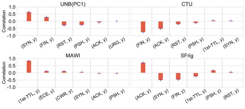
Figure 3. Top 6 correlation between each value in packet headers and ground truth ($y$).

Relative importance of specific header flags:

Figure 3 shows that certain packet header fields can be particularly useful for novelty detection, depending on the anomaly; these results are evident in the results. One of the more important findings from taking a closer look at the correlations between features and ground truth is that the most important packet header values will depend on the novelty detection problem. We explore this in more detail below.

Attack detection:

In the case of the UNB dataset, we see that the SYN flag can be very useful in identifying novelty events related to security, as the SYN flag corresponds to a TCP handshake that occurs at the beginning of the connection and is commonly related to certain types of denial of service attacks, such as a SYN flood. Other packet header information that exhibits correlation include other flags that are commonly associated with denial of service attacks, including the RST and FIN flags, which victim hosts may send in response to a SYN. Traffic flows may also see a novel distribution of packets with ACK flags, given that packets with ACK flags are sent in response to SYN packets, which are sent either to initiate a new flow or as part of an attack (e.g., a SYN flood attack). Such a situation is the case with CTU (novel infected device) where we see high correlation for FIN, ACK, and RST flags. In all of these cases, an increase in packets that include these flags could likely correspond with a volumetric denial of service attack, such as a SYN flood.

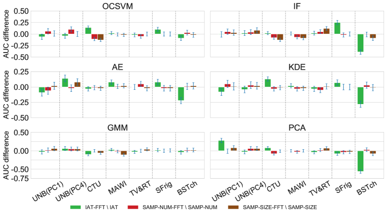
Figure 4. Difference in AUC for FFT vs. raw time series representations.

Novel device detection:

The MAWI dataset, where the novelty detection problem involves detecting a novel device, finds the TTL field in a packet header to be significant. This result also follows intuition, as the TTL value is often a coarse indicator of network topology (i.e., how many network-level “hops” a device is from a particular destination endpoint) and naturally two different devices on the network may be located at different network attachment points and thus be different distances away from common network locations. Such topological differences would be apparent in the TTL field, and a new device attaching at a different location on the network could appear as a sudden influx of network traffic that bears a different distribution in TTL values. In particular, sudden deviations in distributions of TTL values in the dataset may thus reflect the injection of traffic from new devices, or possibly attackers. In the CTU and Lab IoT datasets, the TTL field is comparatively less important because the devices in the dataset were connected on the same local area network, as opposed to different places in the wide area. In such a scenario, the connected devices are a single IP hop away from the monitoring location and thus the TTL values will be the same for all devices. The importance of the SYN field varies across datasets and scenarios, most likely because in some cases the introduction of a new device may involve a change in the distribution of new TCP flows (where the start of each flow is characterized by a SYN packet), whereas in other cases, changes in the number of new flows may not be a useful feature for detecting a novel device.

Novel activity detection:

If someone begins to interact with a connected IoT device in new ways—triggering new types of activities—the traffic itself may bear differences from previously seen traffic. Differences in the traffic itself may arise because activities themselves may bear unique signatures in the underlying network traffic. For example, the amount and nature of traffic generated by opening and closing a refrigerator door in SFrig will generate different types of traffic than the kind of traffic that is generated by activities that do not involve human interaction (e.g., a software update).

These fundamental differences may appear in different ways, such as differences in traffic volume or timing, and in some cases they may appear in the TCP header flags themselves. In the case of SFrig, we see that the ACK flag has a high correlation with ground truth, indicating that changes in the prevalence of ACKs (i.e., packet acknowledgments) may represent changes in underlying activities. This characteristic likely results from the underlying behavior of TCP, the Internet’s transport protocol, and how it handles packet acknowledgments for flows of different sizes and timings. For example, for large traffic flows, TCP will sometimes optimize its acknowledgment behavior, using techniques such as delayed ACK to improve network performance. Highly interactive behavior and the traffic it generates may exhibit very different qualities than automated traffic (e.g., a software update involving the transfer of a large amount of data) and thus different behavior in ACK traffic. The distribution of ACK fields in the traffic may reflect higher traffic volumes during periods of novel activity. Changes in distributions or frequencies of SYN and FIN packets in the trace can also indicate changes in the number of overall total flows, reflecting novel activities that generate completely new flows or simply change the distribution of active flows. Finally, as stated earlier, the lack of improvement for Sfrig using SAMP-SIZE or STATS features is due to the already high performances achieved under these features on most methods. The same reason applies for the BSTch dataset, where detection is nearly solved under any feature representation.

7.2.3. Fourier Domain Representation

We compare Fourier domain representations (obtained by Fast Fourier Transforms (FFT), where we retain as many FFT components as the number of time points) to raw time series representations of each flow, namely IAT, SAMP-NUM, and SAMP-SIZE. Figure 4 presents the difference in AUC, i.e., the AUC obtained under FFT minus that obtained under the corresponding raw time series representation.

A similar trend is observed across ML procedures: apart for a few device datasets (e.g., positive effects in SFrig, and in UNB (PC1, PC4) — under AE and PCA — and negative effect in BSTch with respect to IAT), FFT genrally makes no significant difference in the achieved AUC over raw time series. In other words, the various ML procedures seem able to extract much of the same information already from the raw time series, as their internal representations of the data already account for major trends in the times series and thus do away with the need to preprocess through FFT.

8. Conclusion

The performance of novelty detection in computer networking requires careful decisions about how to best represent traffic data, e.g, which predictive features to extract, which time windows to use, whether to work in time domain or Fourier domain, etc. As we have seen, these choices can significantly affect detection accuracy and depend specifically on the the types of novelty we seek to detect and the machine learning model being used.

Unfortunately, despite much past work on anomaly detection in networking, we have no general guiding principles towards predictive yet succinct traffic data representation. Indeed, past work in this area has focused on solutions to individual problems, with application of a specific model (e.g., PCA) to a particular representation (e.g., IPFIX/NetFlow). Without a general framework, researchers and practitioners must apply heuristics to select models, model parameters and representations, a problem which is further exacerbated by the general lack of automation of these common preprocessing steps. As a result, each problem in networking that seeks to address anomaly detection (or, more generally, novelty detection) must re-invent the wheel, developing bespoke techniques for each step and generating pipelines that are difficult to reproduce.

To address these difficulties, we have developed and released an open-source library and command-line tool, netml, that extracts common features from network packet captures. The tool is configurable to allow for specific application choices of features, yet simply to use and upgrade to incorporate state of the art models and representations. For example, we have recently extended the library to develop and test a fast, online OCSVM specifically designed for network anomaly detection settings. It is our hope and expectation that these types of tools will facilitate more such research across the network measurement and machine learning communities.

Appendix A Further Information on Datasets

Table A.1. Data representation dimensions for each dataset.

Device	[c]IAT, IAT-FFT	[c]SIZE, SIZE-FFT	[c]STATS	[c]SAMP-NUM, SAMP-NUM-FFT, SAMP-SIZE
PC1	14	15	10	14
PC2	16	17	10	16
PC3	16	17	10	16
PC4	19	20	10	19
PC5	15	16	10	15
2Rsps	12	13	10	12
2PCs	35	36	10	35
TV&RT	12	13	10	12
GHom	19	20	10	19
SCam	6	7	10	6
SFrig	30	31	10	30
BSTch	148	149	10	148

Table A.2. Train, Validation, and Test set, in which ’N’ represents normal and ’A’ represents novelty (e.g., attack, novel device, and novel activity). Validation set is only used for picking the best parameters for each algorithm and its size is a quarter of the size of each test set.

Reference	Devices	Train set	Validation set	Test set
UNB IDS	PC1	N: 5000	N: 35, A: 35	N: 144, A: 144
	PC2	N: 5000	N: 51, A: 51	N: 206, A: 206
	PC3	N: 5000	N: 44, A: 44	N: 177, A: 177
	PC4	N: 5000	N: 42, A: 42	N: 168, A: 167
	PC5	N: 5000	N: 72, A: 72	N: 288, A: 288
CTU IoT	2Rsps	N: 5000	N: 100, A: 100	N: 400, A: 400
MAWI	2PCs	N: 5000	N: 100, A: 100	N: 400, A: 400
Lab IoT	TV&RT	N: 4636	N: 69, A: 69	N: 277, A: 277
	GHom	N: 5000	N: 100, A: 100	N: 400, A: 400
	SCam	N: 5000	N: 40, A: 40	N: 161, A: 161
	SFrig	N: 2952	N: 59, A: 59	N: 237, A: 237
	BSTch	N: 997	N: 47, A: 47	N: 189, A: 189

Appendix B Best Parameters: additional datasets and Procedures

B.1. Baseline Results with Best Parameters

Table B.1. AUCs for 4 ML approaches on basic feature representations with best parameters.

Detector	Dataset	[c]STATS	[c]SIZE	[c]IAT	[c]SAMP- NUM
OCSVM	UNB(PC2)	0.59	0.78	0.79	0.80
	UNB(PC3)	0.64	0.86	0.81	0.79
	UNB(PC5)	0.49	0.74	0.80	0.80
	GHom	0.73	0.96	0.69	0.95
	SCam	0.67	0.64	0.53	0.59
IF	UNB(PC2)	0.68	0.59	0.67	0.81
	UNB(PC3)	0.69	0.66	0.69	0.76
	UNB(PC5)	0.58	0.62	0.71	0.78
	GHom	0.88	0.78	0.42	0.96
	SCam	0.64	0.63	0.54	0.63
AE	UNB(PC2)	0.72	0.62	0.73	0.83
	UNB(PC3)	0.78	0.60	0.70	0.80
	UNB(PC5)	0.69	0.68	0.68	0.91
	GHom	0.82	0.66	0.33	0.96
	SCam	0.67	0.46	0.54	0.61
KDE	UNB(PC2)	0.56	0.77	0.79	0.79
	UNB(PC3)	0.62	0.86	0.81	0.79
	UNB(PC5)	0.43	0.71	0.80	0.79
	GHom	0.57	0.96	0.70	0.96
	SCam	0.68	0.63	0.47	0.56
GMM	UNB(PC2)	0.78	0.63	0.71	0.81
	UNB(PC3)	0.87	0.77	0.77	0.81
	UNB(PC5)	0.81	0.72	0.74	0.86
	GHom	0.97	0.96	0.91	0.96
	SCam	0.54	0.64	0.47	0.63
PCA	UNB(PC2)	0.69	0.62	0.43	0.79
	UNB(PC3)	0.71	0.28	0.32	0.81
	UNB(PC5)	0.67	0.30	0.38	0.75
	GHom	0.72	0.40	0.05	0.96
	SCam	0.63	0.61	0.62	0.59

B.2. Effect of Fourier Domain Representation

The figures below show the difference in AUC for the FFT vs. raw timeseries representations with the best model parameters for each model. FFT transformations have little effect on model accuracy.

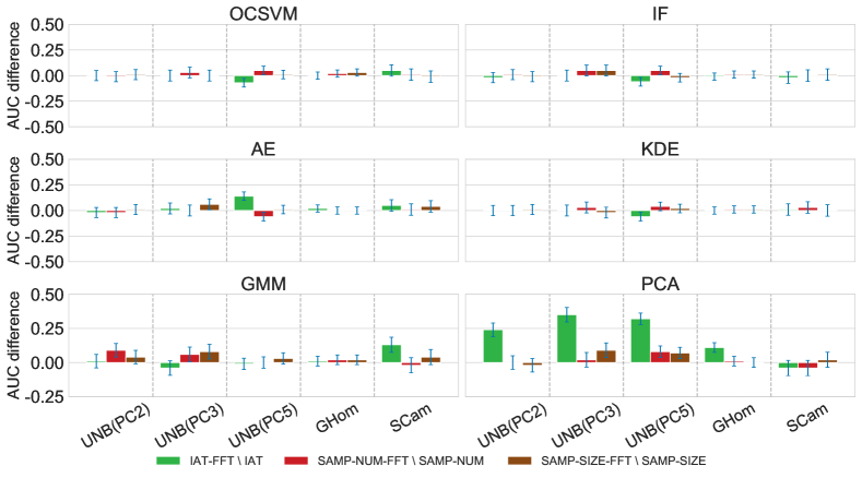
Figure B.1. Difference in AUC for FFT vs. raw time series representations with best parameters.

B.3. Effect of Packet Size Information

The figures below show the difference in AUC for including vs. excluding packet size information for different models: IAT and SAMP. Including packet size can significantly improve model accuracy in certain cases.

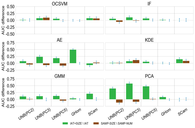
Figure B.2. Differences in AUC due to including vs. excluding packet size information with best parameters.

B.4. Effect of Packet Header

The figures below show the difference in AUC for including vs. excluding packet header information (i.e., IP TTL, TCP flags) for different models: STATS, IAT, and SAMP. Including packet header information almost always improves model accuracy for these models.

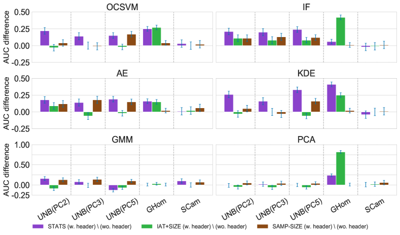
Figure B.3. Differences in AUC due to including vs. excluding packet header information with best parameters.

Appendix C Default Parameters: Additional Datasets and Procedures

C.1. Baseline Results with Default Parameters

Table C.1. AUCs for 4 ML approaches on basic feature representations with default parameters.

Detector	Dataset	[c]STATS	[c]SIZE	[c]IAT	[c]SAMP- NUM
OCSVM	UNB(PC1)	0.48	0.42	0.72	0.76
	UNB(PC2)	0.48	0.37	0.79	0.79
	UNB(PC3)	0.54	0.80	0.82	0.78
	UNB(PC4)	0.55	0.62	0.86	0.75
	UNB(PC5)	0.49	0.64	0.74	0.77
	CTU	0.54	0.77	0.75	0.85
	MAWI	0.28	0.28	0.41	0.58
	TV&RT	1.00	1.00	0.95	0.68
	GHom	0.73	0.96	0.07	0.95
	SCam	0.68	0.46	0.53	0.56
	SFrig	0.88	0.90	0.77	0.95
	BSTch	0.97	0.97	0.93	0.92
IF	UNB(PC1)	0.42	0.52	0.61	0.77
	UNB(PC2)	0.66	0.59	0.68	0.79
	UNB(PC3)	0.69	0.65	0.69	0.76
	UNB(PC4)	0.48	0.51	0.69	0.79
	UNB(PC5)	0.55	0.61	0.68	0.78
	CTU	0.77	0.77	0.86	0.90
	MAWI	0.86	0.68	0.42	0.62
	TV&RT	0.95	0.98	0.90	0.74
	GHom	0.86	0.78	0.42	0.96
	SCam	0.63	0.63	0.50	0.63
	SFrig	0.96	0.95	0.57	0.94
	BSTch	0.94	0.98	0.94	0.96

• *continue

Detector	Dataset	[c]STATS	[c]SIZE	[c]IAT	[c]SAMP- NUM
AE	UNB(PC1)	0.45	0.57	0.65	0.78
	UNB(PC2)	0.64	0.58	0.68	0.81
	UNB(PC3)	0.54	0.42	0.34	0.80
	UNB(PC4)	0.80	0.41	0.37	0.77
	UNB(PC5)	0.70	0.43	0.68	0.80
	CTU	0.29	0.72	0.86	0.83
	MAWI	0.39	0.48	0.43	0.60
	TV&RT	1.00	1.00	0.95	0.76
	GHom	0.88	0.64	0.28	0.96
	SCam	0.48	0.46	0.49	0.60
	SFrig	0.94	0.72	0.72	0.96
	BSTch	0.95	0.87	0.97	0.96
KDE	UNB(PC1)	0.21	0.54	0.69	0.73
	UNB(PC2)	0.56	0.60	0.79	0.78
	UNB(PC3)	0.62	0.77	0.82	0.78
	UNB(PC4)	0.37	0.62	0.86	0.74
	UNB(PC5)	0.34	0.58	0.73	0.78
	CTU	0.75	0.73	0.76	0.92
	MAWI	0.66	0.49	0.39	0.58
	TV&RT	1.00	1.00	0.95	0.67
	GHom	0.57	0.94	0.05	0.95
	SCam	0.68	0.64	0.47	0.56
	SFrig	0.94	0.91	0.74	0.95
	BSTch	0.96	0.96	0.94	0.91

Table C.2. AUCs for 2 additional ML approaches (GMM and PCA) on basic feature representations with default parameters.

Detector	Dataset	[c]STATS	[c]SIZE	[c]IAT	[c]SAMP- NUM
GMM	UNB(PC1)	0.36	0.22	0.62	0.79
	UNB(PC2)	0.59	0.55	0.70	0.79
	UNB(PC3)	0.63	0.11	0.74	0.80
	UNB(PC4)	0.54	0.59	0.65	0.82
	UNB(PC5)	0.81	0.41	0.70	0.78
	CTU	0.69	0.70	0.52	0.89
	MAWI	0.66	0.40	0.48	0.62
	TV&RT	0.99	0.93	0.90	0.90
	GHom	0.39	0.51	0.67	0.96
	SCam	0.63	0.62	0.42	0.63
	SFrig	0.79	0.91	0.69	0.96
	BSTch	0.94	0.08	0.93	0.96
PCA	UNB(PC1)	0.33	0.21	0.30	0.72
	UNB(PC2)	0.58	0.55	0.41	0.80
	UNB(PC3)	0.62	0.15	0.29	0.79
	UNB(PC4)	0.42	0.27	0.54	0.70
	UNB(PC5)	0.39	0.22	0.39	0.75
	CTU	0.69	0.70	0.74	0.89
	MAWI	0.66	0.40	0.40	0.58
	TV&RT	0.99	0.99	0.96	0.61
	GHom	0.40	0.42	0.06	0.96
	SCam	0.63	0.62	0.60	0.57
	SFrig	0.79	0.90	0.69	0.95
	BSTch	0.97	0.08	0.92	0.95

C.2. Effect of Fourier Domain Representation

The figures below show differences in model accuracy for Fourier domain representation vs. raw timeseries representations for different models and datasets. Fourier domain representations in general do not improve model accuracy.

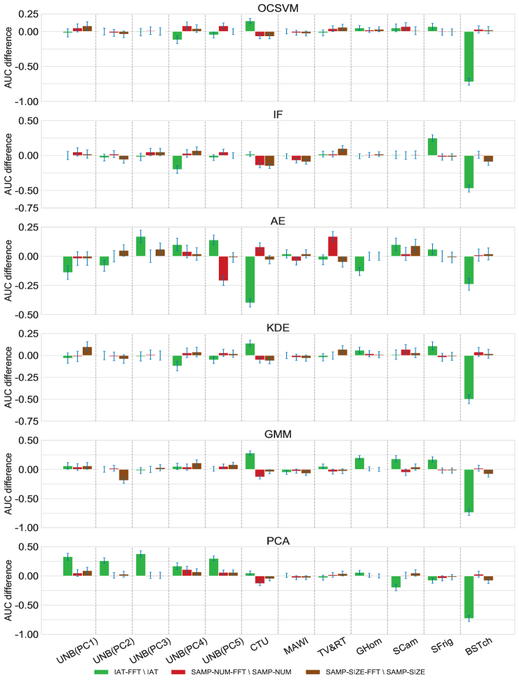
Figure C.1. Difference in AUC for FFT vs. raw time series representations with default parameters.

C.3. Effect of Packet Size Information

The figures below show differences in model accuracy as a result of including packet size information for different models and datasets. Packet size information generally improves model accuracy.

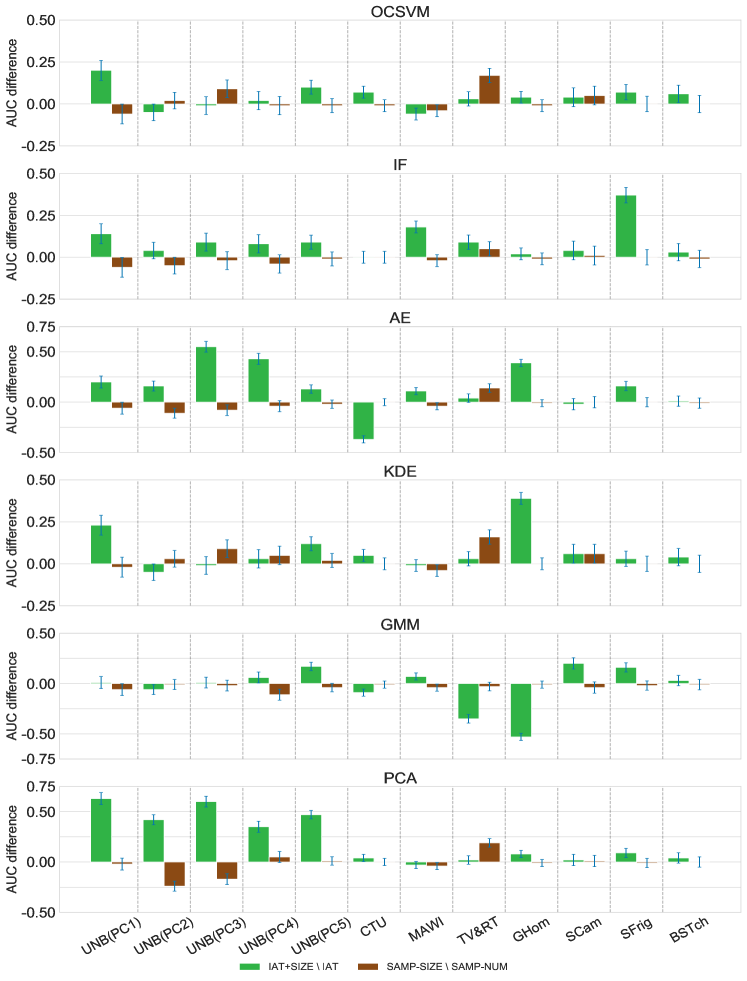
Figure C.2. Differences in AUC due to including vs. excluding packet size information with default parameters.

C.4. Effect of Packet Header

The figures below show differences in model accuracy as a result of including packet header information for different models and datasets. Packet header information generally improves model accuracy.

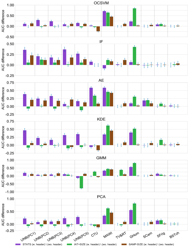
Figure C.3. Differences in AUC due to including vs. excluding packet header information with default parameters.

References

- [1] Removed for anonymity.
- [2] C. C. Aggarwal. Outlier analysis. In Data mining, pages 237–263. Springer, 2015.
- [3] S. A. Aljawarneh and R. Vangipuram. Garuda: Gaussian dissimilarity measure for feature representation and anomaly detection in internet of things. The Journal of Supercomputing, pages 1–38, 2018.
- [4] R. Bhatia, S. Benno, J. Esteban, T. Lakshman, and J. Grogan. Unsupervised machine learning for network-centric anomaly detection in iot. In Proceedings of the 3rd ACM CoNEXT Workshop on Big DAta, Machine Learning and Artificial Intelligence for Data Communication Networks, pages 42–48, 2019.
- [5] C. M. Bishop. Pattern recognition and machine learning. springer, 2006.
- [6] R. Doshi, N. Apthorpe, and N. Feamster. Machine learning ddos detection for consumer internet of things devices. In 2018 IEEE Security and Privacy Workshops (SPW), pages 29–35. IEEE, 2018.
- [7] R. F. Fouladi, C. E. Kayatas, and E. Anarim. Frequency based ddos attack detection approach using naive bayes classification. In 2016 39th International Conference on Telecommunications and Signal Processing (TSP), pages 104–107. IEEE, 2016.
- [8] T. M. W. Group. ”mawi wide dataset”. https://mawi.wide.ad.jp/mawi/, 2019. Accessed: 2019-12-13.
- [9] G. Gu, R. Perdisci, J. Zhang, and W. Lee. Botminer: Clustering analysis of network traffic for protocol-and structure-independent botnet detection. 2008.
- [10] D. H. Hoang and H. D. Nguyen. A pca-based method for iot network traffic anomaly detection. In 2018 20th International conference on advanced communication technology (ICACT), pages 381–386. IEEE, 2018.
- [11] H. Jiang, J. Jang, and S. Kpotufe. Quickshift++: Provably good initializations for sample-based mean shift. arXiv preprint arXiv:1805.07909, 2018.
- [12] A. Kumar, A. Abdelhadi, and C. Clancy. Novel anomaly detection and classification schemes for machine-to-machine uplink. In 2018 IEEE International Conference on Big Data (Big Data), pages 1284–1289. IEEE, 2018.
- [13] A. Lakhina, M. Crovella, and C. Diot. Diagnosing network-wide traffic anomalies. ACM SIGCOMM, 34(4):219–230, 2004.
- [14] A. Lakhina, M. Crovella, and C. Diot. Mining anomalies using traffic feature distributions. ACM SIGCOMM, 35(4):217–228, 2005.
- [15] A. Lakhina, K. Papagiannaki, M. Crovella, C. Diot, E. D. Kolaczyk, and N. Taft. Structural analysis of network traffic flows. In ACM SIGMETRICS, pages 61–72, 2004.
- [16] A. H. Lashkari, A. F. A. Kadir, L. Taheri, and A. A. Ghorbani. Toward developing a systematic approach to generate benchmark android malware datasets and classification. In 2018 International Carnahan Conference on Security Technology (ICCST), pages 1–7. IEEE, 2018.
- [17] L. J. Latecki, A. Lazarevic, and D. Pokrajac. Outlier detection with kernel density functions. In International Workshop on Machine Learning and Data Mining in Pattern Recognition, pages 61–75. Springer, 2007.
- [18] F. S. d. Lima Filho, F. A. Silveira, A. de Medeiros Brito Junior, G. Vargas-Solar, and L. F. Silveira. Smart detection: An online approach for dos/ddos attack detection using machine learning. Security and Communication Networks, 2019, 2019.
- [19] F. T. Liu, K. M. Ting, and Z.-H. Zhou. Isolation-based anomaly detection. ACM Transactions on Knowledge Discovery from Data (TKDD), 6(1):3, 2012.
- [20] Y. Meidan, M. Bohadana, Y. Mathov, Y. Mirsky, A. Shabtai, D. Breitenbacher, and Y. Elovici. N-baiot—network-based detection of iot botnet attacks using deep autoencoders. IEEE Pervasive Computing, 17(3):12–22, 2018.
- [21] Y. Mirsky, T. Doitshman, Y. Elovici, and A. Shabtai. Kitsune: an ensemble of autoencoders for online network intrusion detection. arXiv preprint arXiv:1802.09089, 2018.
- [22] A. Moore, D. Zuev, and M. Crogan. Discriminators for use in flow-based classification. Queen Mary and Westfield College, Department of Computer Science, (August), 2005.
- [23] T. U. of New Brunswick. The CICIDS2017 Dataset. https://www.unb.ca/cic/datasets/ids-2017.html, 2017. Accessed: 2019-12-13.
- [24] A. V. Oppenheim. Discrete-time signal processing. Pearson, 1999.
- [25] A. Paszke, S. Gross, F. Massa, A. Lerer, J. Bradbury, G. Chanan, T. Killeen, Z. Lin, N. Gimelshein, L. Antiga, A. Desmaison, A. Kopf, E. Yang, Z. DeVito, M. Raison, A. Tejani, S. Chilamkurthy, B. Steiner, L. Fang, J. Bai, and S. Chintala. Pytorch: An imperative style, high-performance deep learning library. In H. Wallach, H. Larochelle, A. Beygelzimer, F. d'Alché-Buc, E. Fox, and R. Garnett, editors, Advances in Neural Information Processing Systems 32, pages 8024–8035. Curran Associates, Inc., 2019.
- [26] R. Perdisci, W. Lee, and N. Feamster. Behavioral clustering of http-based malware and signature generation using malicious network traces. In NSDI, volume 10, page 14, 2010.
- [27] A. Ramachandran, N. Feamster, and S. Vempala. Filtering spam with behavioral blacklisting. In ACM conference on computer and communications security (CCS), pages 342–351, 2007.
- [28] H. Ringberg, A. Soule, J. Rexford, and C. Diot. Sensitivity of pca for traffic anomaly detection. In ACM SIGMETRICS, pages 109–120, 2007.
- [29] B. I. Rubinstein, B. Nelson, L. Huang, A. D. Joseph, S.-h. Lau, S. Rao, N. Taft, and J. Tygar. Stealthy poisoning attacks on pca-based anomaly detectors. ACM SIGMETRICS Performance Evaluation Review, 37(2):73–74, 2009.
- [30] Scapy. ”scapy”. https://scapy.net/index, 2019. Accessed: 2019-12-13.
- [31] B. Schölkopf, R. C. Williamson, A. J. Smola, J. Shawe-Taylor, and J. C. Platt. Support vector method for novelty detection. In Advances in neural information processing systems, pages 582–588, 2000.
- [32] D. W. Scott and S. R. Sain. Multidimensional density estimation. Handbook of statistics, 24:229–261, 2005.
- [33] G. Thamilarasu and S. Chawla. Towards deep-learning-driven intrusion detection for the internet of things. Sensors, 19(9):1977, 2019.
- [34] C. T. University. ”malware on iot dataset”. https://www.stratosphereips.org/datasets-iot, 2019. Accessed: 2019-12-13.
- [35] Y. Zhao, Z. Nasrullah, and Z. Li. Pyod: A python toolbox for scalable outlier detection. Journal of Machine Learning Research, 20(96):1–7, 2019.
- [36] C. Zhou and R. C. Paffenroth. Anomaly detection with robust deep autoencoders. In Proceedings of the 23rd ACM SIGKDD International Conference on Knowledge Discovery and Data Mining, pages 665–674. ACM, 2017.