Inference in Difference-in-Differences with Few Treated Units and Spatial Correlation

We consider the problem of inference in Difference-in-Differences (DID) when there are few treated units and errors are spatially correlated. We first show that, when there is a single treated unit, some existing inference methods designed for settings with few treated and many control units remain asymptotically valid when errors are weakly dependent. However, these methods may be invalid with more than one treated unit. We propose alternatives that are asymptotically valid in this setting, even when the relevant distance metric across units is unavailable.

Keywords: hypothesis testing; causal inference; randomization inference; permutation tests

JEL Codes: C12; C21; C23; C33

1 Introduction

Difference-in-Differences (DID) presents a series of challenges for inference. There is a large number of inference methods for DID. However, the effectiveness of different solutions depends crucially on the set of assumptions one is willing to make on the errors, and on many features of the empirical design, such as the number of treated and control units. A non-exhaustive list of papers that proposed and/or analyzed different inference methods for DID in different settings include Arellano, Bertrand04howmuch, Donald, cameron2008bootstrap, CT, Bester2011, Muller2016, IZA, Canay, FP, MW, ferman2019simple; FermanJAE, Roth2020, Athey2022 and alvarez2023extensions.

We consider a common setting in which a satisfactory solution is not yet available: when (i) there is a small number of treated units, (ii) the number of periods is fixed, and (iii) errors are possibly spatially correlated, but the relevant distance metric is not available to the applied researcher. Throughout, we refer to “spatial correlation” as any correlation in the cross section, not necessarily related to a geographical distance metric.

CT (henceforth, CT) and FP (henceforth, FP) proposed inference methods for settings with few treated and many control units, when there is a fixed number of pre-treatment periods. However, they derive the validity of these methods assuming independence across units (or a spatial correlation depending on an observed distance metric). Considering first a setting with a single treated unit, we derive conditions in which these methods remain asymptotically valid in the presence of spatial correlation, even when the relevant distance metric across units is not available. The main assumptions are that (i) the post-pre difference in average errors for each unit has the same marginal distribution for all units — we can relax this assumption by allowing for heteroskedasticity with a known structure that can be estimated —, and (ii) the cross-section distribution of this post-pre difference in average errors is weakly dependent for the control units. Under these conditions, the asymptotic distribution of the DID estimator depends only on the post-pre difference in average errors of the treated unit. Moreover, the residuals of the control units asymptotically recover the distribution of the errors of the treated unit, even when there is spatial correlation.

However, when there is more than one treated unit, we show that these inference methods proposed by CT and FP may not be asymptotically valid if there is spatial correlation, and the applied researcher does not have information on the relevant distance metric. The intuition is clear: when we (mistakenly) assume that errors are independent across clusters, we underestimate the volatility of the average of the errors for the treated units if errors are positively correlated across the treated units.

We propose alternatives that are asymptotically valid, though generally conservative, in this setting. We first consider an aggregate of the treated units, and derive critical values based on a worst-case scenario for the spatial correlation. While this guarantees a test that is asymptotically valid when the number of control units increases (with the number of treated units fixed), the cost of being robust to unobserved spatial correlation among the treated units is a potential loss in terms of power. For settings in which the outcome variable is the aggregate of unit $\times$ time individual-level observations, we consider a second alternative. We again consider the aggregation of the $N_{1}$ treated units. However, we show that, in this case, we can use information on the within-unit correlation to bound the spatial correlation between treated units. Under the assumption that two individuals within the same unit are relatively more correlated than two individuals in different units, we show that it is possible construct a test that is still robust to spatial correlation, but with a lower loss in terms of power.

Finally, we also consider a third alternative, where we consider separate regressions for each treated unit, and adjust the $p$-values using a multiple hypotheses testing (MHT) procedure that imposes few to no assumptions on the dependence between tests. In this case, one may invert the multiple testing procedure to produce valid confidence sets on the heterogeneous effects, and project these to obtain confidence sets on average effects. While this alternative imposes fewer assumptions on the errors, this comes at a cost: we show that this approach produces confidence sets that contain the confidence intervals obtained by our other alternatives.

We analyze a Monte Carlo simulation based on the spatial correlation structure of the American Community Survey (ACS). We then revisit the work by Sommers, who analyzed the effects of the Massachusetts 2006 health reform, in light of our results.

2 Setting

Let $Y_{st}(0)$ ($Y_{st}(1)$) be the potential outcome of unit $s$ at time $t$ when this unit is untreated (treated) at this period. We consider that potential outcomes are given by

$$\begin{cases}Y_{st}(0)=\theta_{s}+\gamma_{t}+\eta_{st}\\ Y_{st}(1)=\alpha_{st}+Y_{st}(0),\end{cases}$$ (1)

where $\alpha_{st}$ is the (possibly heterogeneous) treatment effects for unit $s$ at time $t$, $\theta_{s}$ are time-invariant unobserved effects, and $\gamma_{t}$ are group-invariant unobserved effects. The error term $\eta_{st}$ represents unobserved determinants of $Y_{st}(0)$ that are not captured by the fixed effects. We observe $Y_{st}=d_{st}Y_{st}(1)+(1-d_{st})Y_{st}(0)$, where $d_{st}$ is a dummy variable equal to one if unit $s$ is treated at time $t$. We can also consider the case in which we observe individual-level observations $Y_{ist}$. In this case, a solution to take within-(unit $\times$ time) correlations into account is to consider unit $\times$ time aggregates $Y_{st}$. Therefore, we focus on the unit $\times$ time aggregate setting.

We focus on the case in which treatment is non-reversible and starts for all treated units after date $t^{\ast}$ (see Remark 4.4 for the case with variation in adoption time). There are $N_{1}$ treated units, $N_{0}$ control units, and $T$ time periods. Let $\mathcal{I}_{1}$ ($\mathcal{I}_{0}$) be the set of indices for treated (control) units, while $\mathcal{T}_{1}$ ($\mathcal{T}_{0}$) be the set of indices for post- (pre-) treatment periods. We treat the allocation of the treatment as fixed. We also treat $\{\alpha_{st}\}_{s\in\mathcal{I}_{1},t\in\mathcal{T}_{1}}$ as fixed parameters, and define $\alpha\equiv\frac{1}{N_{1}}\frac{1}{T-t^{\ast}}\sum_{s\in\mathcal{I}_{1}}\sum_{t\in\mathcal{T}_{1}}\alpha_{st}$, which is the average treatment effects across treated units and treated periods. Since $\theta_{s}$ and $\gamma_{t}$ are eliminated when we include the fixed effects, we do not need to impose any constrain on those variables, which can be treated either as fixed or stochastic. Therefore, the only relevant uncertainty in our setting comes from potentially different realizations of unobserved variables $\eta_{st}$. This may include, for example, unit $\times$ time specific weather or economics unobserved shocks. Moreover, it may be that such unobserved variables are serially correlated and/or correlated across units.

A framework in which treatment assignment and treatment effects are treated as fixed is common in the literature of DID with few treated clusters, as considered by CT, FP, and alvarez2023extensions. A similar framework is also considered in other settings in which the number of treated clusters is fixed, such as in the synthetic controls literature (Abadie2010; SDID; ASC; BF; CWZ; FP_QE; Ferman_JASA; Wang). In such settings, we want to learn about the realized treatment effects for the units that received treatment ($\{\alpha_{st}\}_{s\in\mathcal{I}_{1},t\in\mathcal{T}_{1}}$), while uncertainty comes from different realizations of unobserved variables, such as weather or economic unobserved shocks.

Let $W_{s}=\frac{1}{T-t^{\ast}}\sum_{t\in\mathcal{T}_{1}}\eta_{st}-\frac{1}{t^{\ast}}\sum_{t\in\mathcal{T}_{0}}\eta_{st}$, which is the post-pre difference in average errors for each unit $s$. In this case in which treatment starts at the same period for all treated units, the DID estimator is numerically equivalent to the two-way fixed effects (TWFE) estimator, which is given by

$$\widehat{\alpha} =\frac{1}{N_{1}}\sum_{s\in\mathcal{I}_{1}}\left[\frac{1}{T-t^{\ast}}\sum_{t\in\mathcal{T}_{1}}Y_{st}-\frac{1}{t^{\ast}}\sum_{t\in\mathcal{T}_{0}}Y_{st}\right]-\frac{1}{N_{0}}\sum_{s\in\mathcal{I}_{0}}\left[\frac{1}{T-t^{\ast}}\sum_{t\in\mathcal{T}_{1}}Y_{st}-\frac{1}{t^{\ast}}\sum_{t\in\mathcal{T}_{0}}Y_{st}\right]$$ (2)

$$=\alpha+\frac{1}{N_{1}}\sum_{s\in\mathcal{I}_{1}}W_{s}-\frac{1}{N_{0}}\sum_{s\in\mathcal{I}_{0}}W_{s}.$$

We consider the following identification assumption.

Assumption 2.1.

$\mathbb{E}\left[W_{s}\right]=0$ for all $s\in\mathcal{I}_{1}\cup\mathcal{I}_{0}$.

We recall that treatment assignment is fixed, so this assumption means that the post-pre difference in average errors has the same mean for both treated and control units. This assumption is implied by a standard parallel trends assumption for all periods, and is equivalent to assuming a parallel trends assumption on the potential outcomes. We can extend our results to consider alternative parallel trends assumptions (Marcus) and alternative estimators.

Given Assumption 2.1, we have that $\mathbb{E}[\widehat{\alpha}]=\alpha$, so the DID estimator is unbiased. However, in a setting in which $N_{1}$ is fixed and $N_{0}\rightarrow\infty$, the DID estimator will not be consistent, and will not necessarily be asymptotically normal. In particular, CT show that, under a strong mixing condition on the errors, in this setting $\widehat{\alpha}$ converges in probability to $\alpha+\widetilde{W}$, where $\widetilde{W}\equiv\frac{1}{N_{1}}\sum_{s\in\mathcal{I}_{1}}W_{s}$. Therefore, if we want to test the null hypothesis $H_{0}:\alpha=\alpha_{0}$ at the significance level $\tau$, this would pose some challenges for inference.

3 Inference with independent clusters

Before we move to the case in which errors may be spatially correlated, we start with a brief review of inference methods for settings with few treated clusters, when errors are independent in the cross-section. We focus on the inference approaches proposed by CT and FP for settings with few treated units and a fixed number of periods.

CT propose an interesting inference method in this setting by noting that the residuals $\widehat{W}_{s}$ of the control units may be informative about the distribution of $W_{s}$ for the treated. In their running model, they assume that $W_{s}$ is iid across $s\in\mathcal{I}_{1}\cup\mathcal{I}_{0}$ (Assumption 2 from CT). Note that, under this iid assumption, knowledge about the marginal distribution of $W_{s}$ for the control units implies knowledge about the distribution of $\widetilde{W}$. Therefore, the main idea from CT is to use $\{\widehat{W}_{s}\}_{s\in\mathcal{I}_{0}}$ to approximate the marginal distribution of $W_{s}$ for the treated, and then use that to calculate critical values. More specifically, they propose the following algorithm for testing the null $H_{0}:\alpha=\alpha_{0}$ with a significance level $\tau$.

1Run the DID estimator, and store $\widehat{\alpha}$ and the residuals $\widehat{W}_{s}=\frac{1}{T-t^{\ast}}\sum_{t\in\mathcal{T}_{1}}\hat{\eta}_{st}-\frac{1}{t^{\ast}}\sum_{t\in\mathcal{T}_{0}}\hat{\eta}_{st}$ for all $s\in\mathcal{I}_{0}$ ;

2 for b=1, …, B do

3       Sample with replacement $N_{1}$ values from $\{\widehat{W}_{s}\}_{s\in\mathcal{I}_{0}}$, $(\widehat{W}_{1}^{\ast},...,\widehat{W}_{N_{1}}^{\ast})$ ;

4       Calculate $\widehat{\alpha}_{b}=\frac{1}{N_{1}}\sum_{s=1}^{N_{1}}\widehat{W}_{s}^{\ast}$ ;

5      

Reject the null if $\frac{1}{B}\sum_{b=1}^{B}\mathbf{1}\{|\widehat{\alpha}-\alpha_{0}|>|\widehat{\alpha}_{b}|\}>1-\tau$.

Algorithm 1 CT

Let $\phi_{\mbox{\tiny CT}}$ be an indicator variable equal to one if we reject the null given the algorithm above. We summarize the results from CT in the following proposition.

Proposition (CT).

Suppose we have data on $\{Y_{s1},...,Y_{sT}\}_{\mathcal{I}_{1}\cup\mathcal{I}_{0}}$, and that Assumption 2.1 holds. Assume also that $W_{s}$ is iid across $s$, with a common distribution function $F_{W}$ that has bounded second moment and is absolutely continuous with bounded density. Then, as $N_{0}\rightarrow\infty$ and $N_{1}$ is fixed, (i) $\widehat{\alpha}$ converges in probability to $\alpha+\widetilde{W}$, and (ii) if the null is true, then $\mathbb{E}[\phi_{\mbox{\tiny CT}}]\rightarrow\tau$ as $N_{0},B\to\infty$ at any rate.

Note that CT provide a proof of result (i) under less restrictive conditions (their Proposition 1). Proposition 2 from CT presents result (ii) under similar conditions as we consider here. In particular, assuming that errors are iid in the cross section. CT also consider another alternative for inference in their appendix, in which they relax the iid assumptions, allowing for spatial correlation and heteroskedasticity with a known structure. However, this alternative relies on a known distance metric. It also requires parametrization/estimation of the serial correlation structure, and relies on normality.

FP builds on CT to propose an alternative that allows for heteroskedasticity with a known structure that can be estimated, without requiring parametrization/estimation of the serial correlation structure, and without relying on normality. They consider a setting in which we also observe a vector of covariates $Z_{s}$, and assume that $W_{s}=h(Z_{s},\delta)\xi_{s}$, where $h(\cdot,\delta)$ is a known function with $\delta$ being an unknown parameter, and $\xi_{s}$ is iid for all $s$. In Appendix LABEL:app_plausible_het, we provide evidence that, under the assumption that heteroskedasticity is a sole function of $Z_{s}$, our adopted parametric form for $h$ is reasonable for the dataset used to base our simulations in Section 5, and for the dataset of our empirical illustration in Section 6. Throughout, we consider that the sequence $\{Z_{s}\}_{\mathcal{I}_{1}\cup\mathcal{I}_{0}}$ is fixed. This allows for treated and control units to be arbitrarily different with respect to $Z_{s}$. Therefore, this allows for heteroskedasticity with a known structure (up to a parameter that can be estimated), but still relies on independence across units. In this case, instead of directly sampling from $\{\widehat{W}_{s}\}_{s\in\mathcal{I}_{0}}$, we re-scale the residuals taking into account that they may have different variances. The algorithm to implement their inference method for testing the null $H_{0}:\alpha=\alpha_{0}$ with a significance level $\tau$ is the following.

1Run the DID estimator, and store $\widehat{\alpha}$ and the residuals $\widehat{W}_{s}=\frac{1}{T-t^{\ast}}\sum_{t\in\mathcal{T}_{1}}\hat{\eta}_{st}-\frac{1}{t^{\ast}}\sum_{t\in\mathcal{T}_{0}}\hat{\eta}_{st}$ for all $s\in\mathcal{I}_{0}$ ;

2 Estimate $\delta$ using the residuals from the controls (see example below) ;

3 Compute the normalized residuals $\widehat{\xi}_{s}=\widehat{W}_{s}/h(Z_{s},\widehat{\delta})$, for $s\in\mathcal{I}_{0}$ ;

4 for b=1, …, B do

5       Sample with replacement $N_{1}$ values from $\{\widehat{\xi}_{s}\}_{s\in\mathcal{I}_{0}}$, $(\widehat{\xi}_{1}^{\ast},...,\widehat{\xi}_{N_{1}}^{\ast})$ ;

6      

7      Calculate $\widehat{\alpha}_{b}=\frac{1}{N_{1}}\sum_{s=1}^{N_{1}}h(Z_{s},\widehat{\delta})\widehat{\xi}_{s}^{\ast}$ ;

8      

Reject the null if $\frac{1}{B}\sum_{b=1}^{B}\mathbf{1}\{|\widehat{\alpha}-\alpha_{0}|>|\widehat{\alpha}_{b}|\}>1-\tau$.

Algorithm 2 FP

Let $\phi_{\mbox{\tiny FP}}$ be an indicator variable equal to one if we reject the null given the algorithm above.

Proposition (FP).

Suppose we have data on $\{Y_{s1},...,Y_{sT},Z_{s}\}_{\mathcal{I}_{1}\cup\mathcal{I}_{0}}$, and that Assumption 2.1 holds. Assume also that $W_{s}=h(Z_{s},\delta)\xi_{s}$, where $\xi_{s}$ is iid across $s$, with a common distribution function $F_{\xi}$ that has bounded second moment and is absolutely continuous with bounded density. Assume there exist constants $0<\underline{h}\leq\overline{h}<\infty$, not depending on $N_{0}$, such that $\underline{h}\leq h(Z_{s},\delta)\leq\overline{h}$ for all $s\in\mathcal{I}_{0}\cup\mathcal{I}_{1}$, uniformly as $N_{0}\to\infty$. Assume also that we have an estimator $\hat{\delta}$ of $\delta$ such that $\max_{s\in\mathcal{I}_{0}\cup\mathcal{I}_{1}}|h(Z_{s},\hat{\delta})-h(Z_{s},{\delta})|=o_{p}(1)$ as $N_{0}\to\infty$. Then, (i) $\widehat{\alpha}$ converges in probability to $\alpha+\widetilde{W}$, and (ii) if the null is true, then $\mathbb{E}[\phi_{\mbox{\tiny FP}}]\rightarrow\tau$ as $N_{0},B\to\infty$ at any rate.

This approach is well-suited for settings in which $Y_{st}$ is the state $\times$ time aggregate of individual-level observations $Y_{ist}$. Let $Z_{s}$ be the number of individual-level observations in state $s$. FP consider the case in which heteroskedasticity arises only from variation in the number of observations per unit. In this case, we should expect $\mathbb{V}(W_{s})$ to be a decreasing function of $Z_{s}$. In such cases, the approach from CT would tend to (over-) under-reject when the treated units are (larger) smaller relative to the control units. FP show that, under a wide range of structures on the within-unit correlations, $\mathbb{V}(W_{s})$ would be given by $A+B/Z_{s}$, for parameters $A,B\geq 0$. Note that the bounding conditions on $h(Z_{s},\delta)$ are satisfied in this setting if either $A>0$, or $B>0$ and the sequence $(Z_{s})_{s\in\mathcal{I}_{0}\cup\mathcal{I}_{1}}$ is bounded uniformly as $N_{0}\to\infty$. In this case, the idea is to estimate $A$ and $B$ using the residuals from the control units, and then re-scale the residuals to the control units in order to approximate the marginal distributions of $W_{s}$ for the treated. Then we can use these distributions to compute critical values. This approach can be used when we have access to the individual-level data, or when we have only aggregate data (provided that we have access to information on the number of observations per unit). FP also consider another alternative that allows for spatial correlation, but in this case they would need an asymptotic theory in which the number of pre-treatment periods goes to infinity (see Remark 4.2).

There are other alternatives that are valid with few treated clusters in settings where clusters are independent. Canay and Hagemann2019 propose randomization tests that remain valid under heteroskedasticity, whenever approximate symmetry of the $\{W_{s}\}_{s\in\mathcal{I}_{1}}$ holds. However, in the limiting case where $N_{1}=1$, these tests have either low power or are not defined. MW propose alternative randomization inference tests for few clusters. However, they show in simulations that their method may severely overreject when there is a single treated unit and heteroskedasticity. Hagemann2020 introduces a procedure that is valid under heteroskedasticity when $N_{1}=1$ and the $\{W_{s}\}_{s\in\mathcal{I}_{0}\cup\mathcal{I}_{1}}$ are approximately normal. His approach requires the user pre-specifying an upper bound for the relative variance of the treated $W$ vis-às-vis the variance of the $W$ in the control group. Finally, the wild bootstrap is another common alternative in settings with few independent clusters. However, this method can have poor power when there are few treated units (see, for example, the simulations in Appendix LABEL:Appendix_MC). See Canay2021 for further discussion on the validity of the wild bootstrap with few clusters.

4 Inference with spatial correlation

We consider now the case in which errors may be spatially correlated. We consider the following assumptions.

Assumption 4.1.

(i) $W_{s}=h(Z_{s};\delta)\xi_{s}$, where $\xi_{s}$ is equally distributed for all $s\in\mathcal{I}_{1}\cup\mathcal{I}_{0}$, with a common distribution function $F_{\xi}$ that is absolutely continuous with bounded density; (ii) there exists a constant $\underline{h}>0$ not depending on $N_{0}$ such that $\min_{s\in\mathcal{I}_{0}\cup\mathcal{I}_{1}}h(Z_{s};\delta)\geq\underline{h}$ for all $N_{0}\in\mathbb{N}$; (iii) $\frac{1}{N_{0}}\sum_{s\in\mathcal{I}_{0}}W_{s}\buildrel p\over{\rightarrow}0$ and $\frac{1}{N_{0}}\sum_{s\in\mathcal{I}_{0}}\mathbbm{1}\{\xi_{s}\leq c\}\buildrel p\over{\rightarrow}F_{\xi}(c)$ for every $c\in\mathbb{R}$ when $N_{0}\rightarrow\infty$; and (iv) the estimator $\widehat{\delta}$ for $\delta$ is such that $\max_{s\in\mathcal{I}_{1}\cup\mathcal{I}_{0}}|h(Z_{s};\widehat{\delta})-h(Z_{s};\delta)|=o_{p}(1)$ when $N_{0}\rightarrow\infty$.

Assumptions 4.1(i) and 4.1(ii) restrict the marginal distribution of the treated and control units, as in FP. With this assumption, the residuals of the control units become informative about the distribution of the errors of the treated units, which is the main insight from CT. If we set $h(Z_{s},\delta)$ constant, then these assumptions imply that the marginal distribution $W_{s}$ is the same for both treated and control units, as considered by CT in their running model.

Assumption 4.1(iii) is a high-level assumption that allows for spatially correlated shocks, but restricts such dependence so that we can apply a law of large numbers when we consider the control units. This will be satisfied, for example, if we assume strong mixing conditions in the cross section (see Theorem 3 from JENISH200986). More generally, however, laws of large numbers are known to hold for a wide range of spatially dependent processes (Jenish2012). For simplicity, we refer to this assumption in the text as a weak dependence assumption. Importantly, Assumption 4.1 allows for arbitrary spatial correlation among the treated units. Finally, Assumption 4.1(iv) states that we can consistently estimate the parameters of the heteroskedasticity.

Since we focus on settings in which researchers do not have information on what generates the spatial correlation or they are not willing to assume such structure, we do not need to model in detail the sources of spatial correlation. As a concrete example, we can consider a setting in which the $N_{1}$ treated units are closely located geographically, but we have a larger number of control units in different locations. In this case, if spatial correlation goes to zero when geographical distance increases, then we would have Assumption 4.1(iii) satisfied, even though we may have arbitrarily strong spatial correlation among the $N_{1}$ treated units. While it is natural to think about spatial correlation based on geographical distance, this may not be the case in relevant empirical applications. For example, we may have that units with similar industry shares have more correlated errors. Importantly, we consider a setting in which the applied researcher may be unaware or may not have information on the relevant distance metrics in the cross section, which is common in DID applications (FermanJAE). We further discuss this assumption in Remark 4.3.

Under Assumptions 2.1 and 4.1, it follows again that $\widehat{\alpha}$ is unbiased, and that, when $N_{1}$ is fixed and $N_{0}\rightarrow\infty$, $\widehat{\alpha}$ converges in probability to $\alpha+\widetilde{W}$. We now consider different approaches for testing the null $H_{0}:\alpha=\alpha_{0}$.

4.1 Case with $N_{1}=1$

When $N_{1}=1$, the inference methods proposed by CT and FP can remain valid even if we allow for spatial correlation, and even when we do not have information on the relevant distance metric. The main intuition is that, under Assumption 4.1, the asymptotic distribution of $\widehat{\alpha}$ depends only on $W_{1}$, and the distribution of $W_{1}$ can still be asymptotically approximated using the residuals from the controls, so we can use that to construct critical values.

Let $\widehat{F}_{\xi}(c)={N_{0}}^{-1}\sum_{s\in\mathcal{I}_{0}}\mathbbm{1}\{\widehat{W}_{s}/h(Z_{s},\widehat{\delta})\leq c\}$, where $\widehat{\delta}$ is an estimator for $\delta$. We first show that $\widehat{F}_{\xi}(c)$ approximates the distribution of $\xi_{s}$ if $\widehat{\delta}$ is consistent.

Proposition 4.1.

Suppose Assumptions 2.1 and 4.1 hold. Then, as $N_{0}\rightarrow\infty$, $\widehat{F}_{\xi}(c)$ converges in probability to $F_{\xi}(c)$, uniformly over $c\in\mathbb{R}$.

The proof of Proposition 4.1 is similar to the proof of Proposition 2 from CT. We present details in Appendix LABEL:Proof_N1. In this setting with $N_{1}=1$, the inference method proposed by FP would approximate the asymptotic distribution of $\widehat{\alpha}$ with the empirical distribution of $\{h(Z_{1},\widehat{\delta})\widehat{W}_{s}/h(Z_{s},\widehat{\delta})\}_{s\in\mathcal{I}_{0}}$, to construct the critical values. It immediately follows from Proposition 4.1 that the inference method proposed by FP remains valid for the case with $N_{1}=1$, even when we may have spatial correlation.

Corollary 4.1.

Suppose we have data on $\{Y_{s1},...,Y_{sT},Z_{s}\}_{\mathcal{I}_{1}\cup\mathcal{I}_{0}}$, and that Assumptions 2.1 and 4.1 hold. Then, if $N_{1}=1$ and the null is true, $\mathbb{E}[\phi_{\mbox{\tiny FP}}]\rightarrow\tau$ as $N_{0},B\rightarrow\infty$ at any rate.

Note that if we set $h(Z_{s},\delta)$ constant, and $h(Z_{s},\widehat{\delta})=1$, then Proposition 4.1 and Corollary 4.1 imply that the standard procedure proposed by CT in their running model is also asymptotically valid when $N_{1}=1$ and $N_{0}\rightarrow\infty$, even when we have spatial correlation. The proof of Corollary 4.1 is presented in Appendix LABEL:proof_Cor.

4.2 Case with $N_{1}>1$: inference problems

When $N_{1}>1$, spatial correlation can lead to relevant size distortions if we rely on the methods proposed by CT and FP. For simplicity, consider the case in which $N_{1}=2$, and $\{W_{1},W_{2}\}$ is multivariate normally distributed with correlation $\rho$. Consider also the case in which $h(Z_{s},\delta)$ is constant. Under Assumption 4.1, $\widehat{\alpha}\buildrel p\over{\rightarrow}\alpha+\widetilde{W}$, where $\widetilde{W}\sim N(0,2^{-1}(1+\rho)\mathbb{V}(W_{s}))$. However, if $W_{s}$ is weakly dependent for the control units, when we consider two random draws from $\{\widehat{W}_{s}\}_{s\in\mathcal{I}_{0}}$ to recover the distribution of $\widetilde{W}$, the correlation between these draws would converge to zero when $N_{0}\rightarrow\infty$. As a consequence, the approach proposed by CT would recover a distribution for $\widetilde{W}$ that is normal with a variance $2^{-1}\mathbb{V}(W_{s})$. In this case, critical values would be too small, leading to over-rejection. The same problem applies for the inference method proposed by FP.

The other alternatives for inference discussed in Section 3 would also lead to over-rejection in case the errors of the treated units are positively correlated.

4.3 Case with $N_{1}>1$: alternatives

We consider different alternatives that allows for spatial correlation, even when the applied researcher does not have information on the relevant source of spatial correlation.

4.3.1 Conservative Test 1: worst-case scenario for spatial correlation

We consider first the case in which the errors of all treated units are perfectly correlated as a worst-case scenario to provide an asymptotically valid, though possibly conservative, inference method in this setting. In this case, instead of considering Algorithm 1 or 2, we consider the following alternative.

1Run the DID estimator, and store $\widehat{\alpha}$ and the residuals $\widehat{W}_{s}=\frac{1}{T-t^{\ast}}\sum_{t\in\mathcal{T}_{1}}\hat{\eta}_{st}-\frac{1}{t^{\ast}}\sum_{t\in\mathcal{T}_{0}}\hat{\eta}_{st}$ for all $s\in\mathcal{I}_{0}$ ;

2 Estimate $\delta$ using the residuals from the controls, and compute the normalized residuals $\widehat{\xi}_{s}=\widehat{W}_{s}/h(Z_{s},\widehat{\delta})$, $s\in\mathcal{I}_{0}$ ;

3 for b=1, …, B do

4       Sample one value from $\{\widehat{\xi}_{s}\}_{s\in\mathcal{I}_{0}}$, $\widehat{\xi}^{\ast}$ ;

5      

6      Calculate $\widehat{\alpha}_{b}=\frac{1}{N_{1}}\sum_{s=1}^{N_{1}}h(Z_{s},\widehat{\delta})\widehat{\xi}^{\ast}$ ;

7      

Reject the null if $\frac{1}{B}\sum_{b=1}^{B}\mathbf{1}\{|\widehat{\alpha}-\alpha_{0}|>|\widehat{\alpha}_{b}|\}>1-\tau$.

Algorithm 3 Conservative Test 1

Let $\phi_{\mbox{\tiny cons1}}$ be an indicator variable equal to one if we reject the null given the algorithm above. More specifically, we consider the empirical distribution

$$\widehat{H}(c)=\frac{1}{N_{0}}\sum_{s^{\prime}\in\mathcal{I}_{0}}\mathbbm{1}\{N_{1}^{-1}\sum_{s\in\mathcal{I}_{1}}h(Z_{s},\widehat{\delta})\widehat{\xi}_{s^{\prime}}<c\}.$$

This would recover the asymptotic distribution of $\widehat{\alpha}$ if $\{W_{s}\}_{s\in\mathcal{I}_{1}}$ were perfectly correlated. When treated units are not perfectly correlated, though, we would recover a distribution for $\widehat{\alpha}$ that has a higher variance relative to the true distribution of $\widehat{\alpha}$. Therefore, we can use this distribution to construct critical values that guarantee that, under some assumptions, the test will asymptotically be level $\tau$ regardless of the spatial correlation. To formalize this idea, we consider the following high-level assumption.

Assumption 4.2.

$Pr\left(|\widetilde{W}|>c_{1-\tau}\right)\leq\tau$, where $c_{1-\tau}$ is the $(1-\tau)$-quantile of the distribution of $N_{1}^{-1}\sum_{s\in\mathcal{I}_{1}}h(Z_{s},\delta)|\xi|$.

Consider the simpler case in which $h(Z_{s},\delta)$ is constant. Then this regularity condition simply means that, regardless of the spatial correlation among the treated units, the probability of having extreme values for the average of the treated units, $\widetilde{W}$, is weakly smaller than the probability of having extreme values for a single draw of $W_{s}$.

Note that Assumption 4.2 is satisfied if $\{W_{s}\}_{s\in\mathcal{I}_{1}}$ is multivariate normal. In this case, $\widetilde{W}$ would also be normally distributed, and we have that $\mathbb{V}(\widetilde{W})\leq\mathbb{V}(W_{s})$ irrespectively of the spatial correlation among the treated units. Therefore, $\widetilde{W}$ will be less likely to attain extreme values than $W_{s}$. This is valid for any value of the spatial correlation, even when treated units are negatively correlated. The same intuition remains valid if $h(Z_{s},\delta)$ is not constant.

If we relax the condition that $\{W_{s}\}_{s\in\mathcal{I}_{1}}$ is multivariate normal, then we still have that $\mathbb{V}(\widetilde{W})\leq\mathbb{V}(W_{s})$. However, this does not necessarily guarantee that Assumption 4.2 holds in this case. Still, since the marginal distributions of $\{W_{s}\}_{s\in\mathcal{I}_{1}}$ are identified (Proposition 4.1), it is possible to check whether Assumption 4.2 is reasonable in a given empirical setting. We show in Appendix LABEL:App_copulas that it is possible to search over the space of copulas for the worst-case scenario for $Pr\left(|\widetilde{W}|>c_{1-\tau}\right)$, given the marginal distributions of $\{W_{s}\}_{s\in\mathcal{I}_{1}}$. For the dataset we used to base our simulations from Section 5, we searched over 100,000 Gaussian copulas, holding fixed the marginal distributions of $W_{s}$, and we show that in all of those cases the joint distribution of $\{W_{1},...,W_{N_{1}}\}$ would satisfy Assumption 4.2. In those simulations, we allow for complex dependencies between treated units, in which, for example, the conditional expectation function (CEF) of $W_{1}$ given $W_{2}$ is non-monotonic (in contrast to the setting with $\{W_{1},...,W_{N_{1}}\}$ multivariate normal, in which this CEF would necessarily be linear). Therefore, these simulations provide evidence that Assumption 4.2 is a reasonable approximation to the data used to construct our simulations. We find a similar conclusion in the dataset used in our empirical illustration in Section 6. In case we find copulas such that $Pr\left(|\widetilde{W}|>c_{1-\tau}\right)>\tau$, so Assumption 4.2 would not necessarily be satisfied, we also show how one could correct critical values so that the test remains valid whenever the true dependence structure is less conservative than the most conservative copula considered.

It follows directly from Proposition 4.1 and Assumption 4.2 that this modified test asymptotically controls for size under these assumptions.

Proposition 4.2.

Suppose we have data on $\{Y_{s1},...,Y_{sT},Z_{s}\}_{\mathcal{I}_{1}\cup\mathcal{I}_{0}}$, and that Assumptions 2.1, 4.1, and 4.2 hold. Then, if the null is true, $\limsup_{N_{0},B\rightarrow\infty}\mathbb{E}[\phi_{\mbox{\tiny cons1}}]\leq\tau$, where $N_{0},B\rightarrow\infty$ at any rate.

Therefore, this conservative test provides a viable alternative in settings where $N_{1}<<N_{0}$ that is robust to weakly dependent spatial correlation. While we guarantee that this modified test does not over-reject (asymptotically), it will generally be conservative when $N_{1}>1$, unless the errors of treated units are perfectly correlated.

Remark 4.1.

If a distance metric is available and the researcher is willing to assume such distance metric is the relevant one for the spatial correlation, then other available alternatives might present better power (for example, the inference method proposed in the Appendix of CT). In this case, there would be a trade-off between a test that is more powerful but requires correct specification of the spatial correlation, versus a test that is less powerful, but does not require correct specification of the spatial correlation (or even the observation of a distance metric in the cross section).

Remark 4.2.

Related to Remark 4.1, another alternative to provide a more powerful test may be to infer about the spatial correlation using the time series. For example, VOGELSANG2012303 and CWZ. FP also propose an alternative inference method in their section IV (not the one we reviewed in Section 3) that allows for spatial correlation. However, such alternatives would require a large time series, while the alternatives we propose remain valid even when we have only one pre- and one post-treatment period. Given the survey from Roth, settings in which the time series dimension is short are prevalent in DID applications.

Remark 4.3.

The assumption that $W_{s}$ is weakly dependent would not be satisfied if there are unobserved shocks affecting a non-negligible fraction of the controls (so that $\frac{1}{N_{0}}\sum_{s\in\mathcal{I}_{0}}W_{s}$ converges in probability to a non-degenerate random variable). In this case, the DID residuals $\widehat{W}_{s}$ would not capture these shocks, and $\widehat{F}_{\xi}(c)$ would underestimate the dispersion of the marginal distribution of $\xi_{s}$. As a consequence, even the conservative test may over-reject. Importantly, however, since the critical values of our conservative test are weakly larger relative to CT or FP, the over-rejection would be no larger than the over-rejection for these other methods. In contrast, a weak dependence assumption may be reasonable when units closer in some distance metric have more correlated errors, but such correlation goes to zero when this distance increases. Such distance metric does not need to coincide with geographical distance (for example, we may have that units with similar industry shares have more correlated errors), and we do not even need to have information on the relevant distance metrics.

Remark 4.4.

Constructing a conservative test becomes more complicated if treated units start treatment at different periods, as we discuss in Appendix LABEL:Appendix_staggered.

4.3.2 Conservative Test 2: bounding the across-unit correlations

For settings in which $Y_{st}$ represents averages of $M_{st}$ individual-level observations $Y_{ist}$, we show that it is possible to construct an alternative test that will generally be less conservative than the Conservative Test 1. The idea is again to consider worst-case scenarios for the spatial correlation, through aggregation of the treated units. In this case, however, we assume that individual-level observations within the same unit are weakly more spatially correlated than individual-level observations in different units. Then, we can use information on the within-unit spatial correlation to bound the across-units spatial correlation. We can consider either the case in which the econometrician observes only unit aggregates $Y_{st}$ (but has information on $M_{st}$) or the case in which individual-level data $Y_{ist}$ is observed. For simplicity, consider the case in which $M_{st}=M_{s}$ for all $t$. We treat the sequence $\{M_{s}\}_{s\in\mathcal{I}_{0}\cup\mathcal{I}_{1}}$ as fixed.

In this setting, FP show that, under a wide range of structures on the within-unit correlations for the individual-level errors, we have that $\mathbb{V}(W_{s})=A+B/M_{s}$ for constants $A,B\geq 0$. Importantly, these parameters are informative about the within-unit correlations, and can be used to bound the across-unit correlations, under the assumption that within-unit correlations are stronger than the across unit ones.

Let $M_{\mbox{\tiny T}}=\sum_{s\in\mathcal{I}_{1}}M_{s}$ be the total number of individual-level observations in the treated units. We consider in this case the DID estimator weighted by $M_{s}$, $\widetilde{\alpha}$, so that

$$\widetilde{\alpha}=\alpha^{\prime}+\frac{1}{M_{\mbox{\tiny T}}}\sum_{s\in\mathcal{I}_{1}}M_{s}W_{s}-\frac{1}{M_{\mbox{\tiny T}}}\sum_{s\in\mathcal{I}_{0}}M_{s}W_{s},$$ (3)

where $\alpha^{\prime}\equiv\frac{1}{M_{\mbox{\tiny T}}}\sum_{s\in\mathcal{I}_{1}}M_{s}\left(\frac{1}{T-t^{\ast}}\sum_{t\in\mathcal{T}_{1}}\alpha_{st}\right)$ is the weighted average treatment effect across units and treated periods. The weighted DID estimator in this case is numerically the same as the DID estimator using the individual-level data (note that all our results are valid whether we have access to the individual-level data, or only to the aggregate data).

We consider a version of Assumption 4.1 for this specific setting. In particular, we consider that the observed covariate driving the heteroskedasticity is $M_{s}$ (the number of individual-level observations), and that $\mathbb{V}(W_{s})=A+B/M_{s}$.

Assumption 4.3.

(i) $W_{s}=\left(A+B/M_{s}\right)^{1/2}\xi_{s}$ for nonnegative constants $A,B$, where $\xi_{s}$ is equally distributed for all $s\in\mathcal{I}_{1}\cup\mathcal{I}_{0}$, with a distribution $F_{\xi}$ that is absolutely continuous with bounded density; there exists $\underline{h}>0$, not depending on $N_{0}$, such that $\min_{j\in\mathcal{I}_{0}\cup\mathcal{I}_{1}}\left\{A+B/M_{j}\right\}\geq\underline{h}$, for all $N_{0}\in\mathbb{N}$; (iii) $\frac{1}{\sum_{s\in\mathcal{I}_{0}}M_{s}}\sum_{s\in\mathcal{I}_{0}}M_{s}W_{s}\buildrel p\over{\rightarrow}0$ and $\frac{1}{N_{0}}\sum_{s\in\mathcal{I}_{0}}\mathbbm{1}\{\xi_{s}\leq c\}\buildrel p\over{\rightarrow}F_{\xi}(c)$ for every $c\in\mathbb{R}$; (iv) the (nonnegative) least squares estimators of $\widehat{W}_{s}^{2}$ on a constant and $1/M_{s}$ using only the control units are consistent for $A$ and $B$ as $N_{0}\to\infty$.

Given Assumption 4.3, we have that $\widetilde{\alpha}\buildrel p\over{\rightarrow}\alpha+\mathcal{W}$, where $\mathcal{W}=\frac{1}{M_{\mbox{\tiny T}}}\sum_{s\in\mathcal{I}_{1}}M_{s}W_{s}$. We propose the following idea for inference: we consider an aggregate treated unit that is the weighted average of the treated units. Then we run FP inference method using this aggregate treated unit and the controls, considering that it has $M_{\mbox{\tiny T}}$ observations. We refer to this test as “Conservative Test 2”. More specifically, we consider the following algorithm.

1Run the weighted DID estimator, and store $\tilde{\alpha}$ and the residuals $\widehat{W}_{s}=\frac{1}{T-t^{\ast}}\sum_{t\in\mathcal{T}_{1}}\hat{\eta}_{st}-\frac{1}{t^{\ast}}\sum_{t\in\mathcal{T}_{0}}\hat{\eta}_{st}$ for all $s\in\mathcal{I}_{0}$ ;

2 Run a (nonnegative) least squares regression of $\widehat{W}_{s}^{2}$ on a constant and $1/M_{s}$, to estimate $\widehat{A}$ and $\widehat{B}$ ;

3 Compute the normalized residuals $\widehat{\xi}_{s}=\widehat{W}_{s}/\sqrt{\widehat{A}+\widehat{B}/M_{s}}$, for $s\in\mathcal{I}_{0}$;

4 for b=1, …, B do

5       Sample $1$ value from $\{\widehat{\xi}_{s}\}_{s\in\mathcal{I}_{0}}$, $\widehat{\xi}^{\ast}$ ;

6       Calculate $\widetilde{\alpha}_{b}=\left(\widehat{A}+\widehat{B}/M_{\mbox{\tiny T}}\right)^{1/2}\widehat{\xi}^{\ast}$ ;

7      

Reject the null if $\frac{1}{B}\sum_{b=1}^{B}\mathbf{1}\{|\widetilde{\alpha}-\alpha_{0}|>|\widetilde{\alpha}_{b}|\}>1-\tau$.

Algorithm 4 Conservative Test 2

Let $\phi_{\mbox{\tiny cons2}}$ be an indicator variable equal to one if we reject the null given the algorithm above.

We assume that individual-level observations within the same unit are weakly more spatially correlated than individual-level observations in different units, which is summarized in the following assumption.

Assumption 4.4.

$\mathbb{V}(\mathcal{W})\leq A+B/{M_{\mbox{\tiny T}}}$.

If we assume that $(W_{1},...,W_{N_{1}})$ is multivariate normal, then this would be sufficient to guarantee that the Conservative Test 2 would be asymptotically conservative. More generally, we consider the following assumption, which is similar to Assumption 4.2.

Assumption 4.5.

$Pr\left(|\mathcal{W}|>c_{1-\tau}\right)\leq\tau$, where $c_{1-\tau}$ is the $(1-\tau)$-quantile of the distribution of $[A+B/M_{\mbox{\tiny T}}]^{1/2}|\xi|$

Similarly to the discussion in Section 4.3.1, Assumption 4.5 is satisfied under joint normality, if Assumption 4.4 holds. More generally, we can also evaluate whether this assumption is plausible by searching over the space of copulas, as we did when evaluating Assumption 4.2. For the datasets we used to base our MC simulations and empirical illustration, we again find that this assumption holds for all the simulated distributions for $(W_{1},...,W_{N_{1}})$, providing evidence that this assumption is reasonable in these applications (details in Appendix LABEL:App_copulas).

Proposition 4.3.

Suppose we have data on $\{Y_{s1},...,Y_{sT},Z_{s}\}_{\mathcal{I}_{1}\cup\mathcal{I}_{0}}$, and that Assumptions 2.1, 4.3, 4.4, and 4.5 hold. Then, if the null is true, $\limsup_{N_{0},B\rightarrow\infty}\mathbb{E}[\phi_{\mbox{\tiny cons2}}]\leq\tau$, where $N_{0},B\rightarrow\infty$ at any rate.

Importantly, since we are bounding the across-unit correlations using information on the within-unit correlations, we expect that this test will be less conservative (and, therefore, have more power) than the Conservative Test 1.

Remark 4.5.

We consider the case in which $M_{st}$ varies across $t$ in Appendix LABEL:Appendix_cons2.

4.3.3 Running $N_{1}$ tests, and correcting for multiple testing

Since CT and FP are valid when $N_{1}=1$ (Corollary 4.1), another alternative for the case with $N_{1}>1$ is to consider $N_{1}$ separate DID regressions — one for each treated unit —, and adjust the inference for multiple testing. In this case, each of the $N_{1}$ hypotheses being tested concerns a treated unit post-treatment average effect, i.e. the $\alpha_{s}=\frac{1}{T-t^{\ast}}\sum_{t\in\mathcal{T}_{1}}\alpha_{st}$ for $s\in\mathcal{I}_{1}$. Since we wish to remain agnostic about spatial correlation, we should use a method that imposes few or no assumptions on the dependence structure between the test statistics. Methods that remain agnostic about the dependence between the tests and that control the family-wise error rate (FWER) involved in multiple testing are provided by the Bonferroni, Holm and Hochberg1988 corrections. Benjamini2001 show that the method provided in Benjamini1995 for controlling the false discovery rate (FDR) in a setting where tests are independent remains valid under positive dependence of the p-values used; they also show that a simple modification of the procedure produces a test that controls FDR and remains valid under arbitrary dependence of the p-values. By combining any of these methods with the results from Section 4.1, we are able to conduct valid inference for each $\alpha_{s}$, $s\in\mathcal{I}_{1}$, while taking into account that we are testing multiple hypotheses.

Once a procedure that controls either the FWER or the FDR is selected, we can also compute a valid $(1-\tau)$ confidence set for the vector of individual treatment effects $(\alpha_{s})_{s\in\mathcal{I}_{1}}$ by test inversion: one collects each vector $(a_{s})_{s\in\mathcal{I}_{1}}\in\mathbb{R}^{N_{1}}$ such that the procedure does not reject any null when testing the nulls $\alpha_{s}=a_{s}$, $s\in\mathcal{N}_{1}$, at significance $\tau$.

Moreover, we can also construct a valid confidence set for the weighted average effect $\alpha_{\omega}=\sum_{s\in\mathcal{N}_{1}}\omega_{s}\alpha_{s}$, where $(\omega_{s})_{s}$ are a set of pre-specified weights. Specifically, we construct this set via projection: we calculate and store $\sum_{s\in\mathcal{I}_{1}}\omega_{s}a_{s}$ for each $(a_{s})_{s\in\mathcal{I}_{1}}$ in the confidence set for individual effects (Scheffe1958; Dufour1990; gafarov2016projection; Freyberger2018). This is equivalent to constructing a confidence set by considering all values $a\in\mathbb{R}$, such that there are null hypotheses $\alpha_{s}=a_{s}$ for $s\in\{1,...,N_{1}\}$ with $\sum_{s\in\mathcal{N}_{1}}\omega_{s}\alpha_{s}=a$, where the multiple hypothesis testing procedure would not reject the null for any null hypotheses $\alpha_{s}=a_{s}$, $s\in\{1,...,N_{1}\}$.

Considering confidence intervals for weighted averages of the treatment effects is interesting, because then we can compare those confidence intervals to the ones generated using the approaches from Sections 4.3.1 and 4.3.2. Whilst the format of the resulting set for average effects is dependent on the correction being employed, when the Bonferroni correction is used, a simple expression is available. In this case, the resulting confidence set is given by:

$$I_{\text{Bonferroni}}(\alpha_{\omega};1-\tau)=\left[\hat{\alpha}_{{\omega}}-\left(\sum_{s\in\mathcal{I}_{1}}\omega_{s}h(Z_{s},\hat{\delta})\right)\hat{q}_{|\xi|}(1-\tau/N_{1}),\hat{\alpha}_{{\omega}}+\left(\sum_{s\in\mathcal{I}_{1}}\omega_{s}h(Z_{s},\hat{\delta})\right)\hat{q}_{|\xi|}(1-\tau/N_{1})\right]\,,$$

where $\hat{\alpha}_{\omega}$ is the weighted TWFE estimator and $\hat{q}_{|\xi|}$ is the empirical quantile function of the absolute value of the rescaled residuals in the control group. In contrast, the confidence set obtained by inverting Conservative Test 1 is given by:

$$I_{\text{Conservative 1}}(\alpha_{\omega};1-\tau)=\left[\hat{\alpha}_{{\omega}}-\left(\sum_{s\in s\in\mathcal{I}_{1}}\omega_{s}h(Z_{s},\hat{\delta})\right)\hat{q}_{|\xi|}(1-\tau),\hat{\alpha}_{{\omega}}+\left(\sum_{s\in\mathcal{I}_{1}}\omega_{s}h(Z_{s},\hat{\delta})\right)\hat{q}_{|\xi|}(1-\tau)\right]\,,$$

which shows that the Conservative Test 1 will always lead to tighter intervals.

At first sight, the result on the conservativeness of the Bonferroni confidence set may appear to be restricted to this correction, and one may wonder whether considering alternative MHT corrections may produce tighter confidence intervals than Conservative Test 1. However, as we show in Appendix LABEL:Appendix_MHT, the confidence interval for the average effect constructed using the Benjamini1995 approach – which is the least conservative method discussed in this section and valid under positive dependence of the p-values used in the tests – contains the confidence interval constructed using Conservative Test 1. This reveals an interesting tradeoff between the methods proposed in Sections 4.3.1 and 4.3.2 and MHT corrections: while agnostic MHT procedures have the advantage of not requiring Assumption 4.2 or 4.5, this comes at a cost of larger confidence intervals.

Finally, we note that, for settings with variation in treatment timing, MHT would have the advantage of circumventing the challenges of implementing Conservative Tests 1 and 2 discussed in Remark 4.4.

5 Simulations with Real Datasets

We analyze the spatial correlation problem, and the proposed conservative tests, in simulations based on the ACS (ipums), at the Public Use Microdata Area (PUMA). We estimate a model for the spatial correlation in which the covariance between two PUMAs may depend on whether they belong to the same state, and on the similarity between their industry compositions. We also allow for heteroskedasticity depending on population sizes (details in Appendix LABEL:Appendix_MC). This way, we can analyze three scenarios: (i) when the applied researcher ignores all spatial correlation; (ii) when he/she considers spatial correlation arising from geographical distance; and (iii) when he/she correctly considers that spatial correlation may arise from both geographical distance and industry composition.

If we consider all pairs of PUMAs, the correlation between their errors in this estimated model is greater (in absolute value) than $0.05$ in only $2.5\%$ of the cases. Therefore, the weak dependence condition we consider seems reasonable in this setting. Still, we have PUMAs with spatial correlation as strong as $0.125$. Therefore, we may have a setting in which the $N_{1}$ treated PUMAs exhibit relevant spatial correlation.

In line with our theoretical model, we consider a setting in which we fix $N_{1}\in\{1,2,\ldots,9,10\}$ PUMAs as the treated ones, and generate multivariate normal draws of $W_{s}$ with this estimated spatial dependence. To illustrate issues related to spatial correlation, we choose the PUMA with the strongest spatial correlation with some other PUMA in our dataset to be treated, and then iteratively assign treatment to $N_{1}-1$ PUMAs in the same state that are most similar in industry composition to previously selected PUMAs. Treatment effects are assumed to be zero. We consider six different inference procedures: (i) the naive version of FP approach (which assumes errors are independent across PUMAs); (ii) a parametric bootstrap that correctly specifies and estimates the heteroskedasticity structure and both sources of spatial correlation (this procedure is similar to the parametric bootstrap suggested in the Appendix of CT); (iii) a misspecified parametric bootstrap that estimates the heteroskedasticity structure due to group sizes and spatial correlation due to being in the same state, but ignores spatial correlation due to industry similarity; (iv) the conservative test presented in Section 4.3.1 (which we refer to as “Conservative Test 1”); (v) the conservative test proposed in Section 4.3.2 (which we refer to as “Conservative Test 2”); and the test function stemming from a CI for the average effect obtained by inversion and projection of the Benjamini1995 MHT procedure discussed in Section 4.3.3. In Appendix LABEL:Appendix_MC, we consider other alternatives, such as inference based on a cluster robust variance estimator (CRVE) and on the wild cluster bootstrap (WCB). These alternatives perform poorly in our setting, both because the number of treated units is very small, and because we have spatial correlation from multiple sources (see, for example, MW_JAE and Djogbenou for discussions on asymptotic approximations for CRVE and WCB).

Figure 1.A presents rejection rates, as a function of $N_{1}$, of tests of the null of no average effect conducted nominally at the 5% significance level, while Figure 1.B presents the ratio between the length of nominal 95% confidence intervals obtained by inverting the corresponding test procedures and the length of a 95% unfeasible confidence interval which uses the true sampling variance of $\widehat{\alpha}$ in the simulations.

Figure 1: MC simulations

A: test size	B: length of CI / length of unfeasible CI

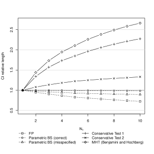
Notes: Figure A presents rejection rates for the six different inference methods we discussed in Section 5, for different values of $N_{1}$. Tests are conducted nominally at the 5% level. Figure B presents information on the ratios between the average length of nominal 95% CIs obtained by test inversion relative to the length of the CI which uses the true sampling variance of $\widehat{\alpha}$.

Overall, these simulations highlight the main messages of the paper: (1) the inference methods proposed by CT and FP remain valid when we have a single treated unit, even when errors are spatially correlated; (2) with $N_{1}>1$, these inference methods over-reject when errors are spatially correlated, and the over-rejection is increasing with $N_{1}$; (3) only accounting for the known sources of spatial correlation, e.g. only controling for state correlation as the misspecified parametric bootstrap does, may not be sufficient to control size; (4) the proposed conservative tests control for size, although they may be conservative when $N_{1}>1$; (5) we are able to provide a less conservative test exploiting the structure of common empirical applications in which units are aggregates of individual-level observations to construct a more powerful test (even if we do not have information on the individual-level observations).

We note that, when $N_{1}=5$, the length of the confidence interval obtained by inverting Conservative Test 2 is only 22% larger than the length of the unfeasible confidence interval. In contrast, Conservative Test 1 has an 85% larger confidence interval than the unfeasible procedure. When $N_{1}=10$, Conservative Test 2 has 33% larger confidence intervals, whereas confidence intervals with Conservative Test 1 are more than 120% larger. The MHT procedure is even more conservative, with confidence intervals 111% (166%) larger when $N_{1}=5$ ($N_{1}=10$). Overall, these numbers illustrate the gains of considering the information on the within-unit correlation to bound the between-unit correlation. Of course, if we have information on all relevant distance metrics in the cross section, then it is possible to correct for spatial correlation with a more powerful test, as the correctly specified parametric bootstrap shows. Still, these simulations illustrate that it is possible to construct valid tests even when such information is unavailable or the researcher is not willing to impose a structure on the spatial correlation.

6 Empirical Illustration

We also illustrate our findings analyzing the effects of the Massachusetts 2006 health care reform. This reform was analyzed by Sommers using a DID design comparing 14 Massachusetts counties with 513 control counties from 45 different states that were selected based on a propensity score to be more similar with the treated counties (we find similar results if we consider a DID regression using all counties, so that there is no pre-selection of control counties). Sommers find a reduction of 2.9%-4.2% in mortality in Massachusetts relative to the controls after the reform (depending on whether covariates are included).

As shown in Figure 1 from Sommers, the outcome variables in the pre-treatment periods followed parallel trajectories when we compare Massachusetts and the control groups. This provides some evidence in favor of Assumption 2.1, although it does not guarantee that. While we do not have strong reasons to believe the parallel trends assumption is violated in this application, we note that this is not crucial for our purposes, since our goal is to analyze alternative inference methods. If we believed there were relevant departures from parallel trends, then, for our purposes, we can simply redefine the target parameters as the treatment effect plus the departure of parallel trends. In this case, for this redefined parameter, Assumption 2.1 would be trivially satisfied, and we can contrast the results from different inference methods.

Sommers relied on standard errors clustered at the state level, which does not work well in this setting with a single treated state. Their inference procedures were then re-analyzed by Kaestner, who considered permutation tests at the county level. While permutation tests are usually considered in a design-based framework, if we consider this approach in our framework, it is asymptotically equivalent to CT at the county level. Therefore, this would also be problematic if counties within the same state are spatially correlated, as we show in Section 4.2. In Appendix LABEL:test, we propose a test for the null that there are relevant state-level shocks. We provide evidence that such spatial correlation is indeed relevant in this application.

We note that this is a setting in which (i) we have only a single treated state, (ii) errors are likely correlated across counties within the same state, and (iii) there is variation in population sizes across counties/states that may lead to heteroskedasticity. If we assume that errors are independent across states, then FP at the state level would be an appropriate inference method in this setting. Moreover, given Corollary 4.1, this inference method remains valid even if we assume that state-level errors are weakly dependent, since in this case we have only a single treated state. We consider, therefore, p-values and CI’s from FP at the state-level as a benchmark. As presented in Table LABEL:Table_Empirical, in this case we fail to reject the null of no effect, for the two outcomes we considered.

While in this application we have a well-defined distance measure for the spatial correlation (which, in this case, is the information on the states), we consider a “thought experiment” in which the applied researcher does not have such information, in order to illustrate our main results. The main advantage is that, in this case, we can contrast our findings with the conclusions based on FP at the state level, which we use as a benchmark.

First, note that we would reject the null if we relied on most of the inference methods that ignore spatial correlation (FP, CRVE and WCB at county level), contrasting with our benchmark results using FP at the state level. This happens because, as discussed in Section 4.2, spatial correlation among the treated units leads to over-rejection. The only exception is CT at the county level. This happens because, while spatial correlation induces over-rejection in this case, the fact that treated counties are relatively larger induces under-rejections. Appendix LABEL:emp_il_alt reports the results for alternative inference methods at both the state and county levels.

We also consider how our conservative tests would perform in this case (again, considering this “thought experiment” in which information on states is unavailable). The conservative tests we propose in Sections 4.3.1 and 4.3.2 present p-values similar to the ones from FP at the state level (our benchmark). When we consider the conservative test proposed in Section 4.3.2, the length of the 95% confidence interval is 43% larger for all cause mortality, and 23% larger for healthcare amenable mortality. Therefore, there is some loss in terms of power, but in settings in which a distance metric is not available, this may be a cost we would have to pay to provide a test that controls for size in the presence of spatial correlation. Moreover, Conservative Tests 1 and 2 offer clear improvements over the procedure based on inverting and projecting the Benjamini1995 correction discussed in Section 4.3.3. Indeed, this procedure leads to CI length around 90% larger than FP at the state level. Overall, results indicate that Conservative Tests 1 and 2 would perform well even if we did not have information on a distance metric, and despite the fact that we have spatial correlation across counties.