Separation of Quark Flavors using DVCS Data

Abstract

Using the available data on deeply virtual Compton scattering (DVCS) off protons and utilizing neural networks enhanced by the dispersion relation constraint, we determine six out of eight leading Compton form factors in the valence quark kinematic region. Furthermore, adding recent data on DVCS off neutrons, we separate contributions of up and down quarks to the dominant form factor, thus paving the way towards a three-dimensional picture of the nucleon.

I Introduction

Understanding the structure of hadrons in terms of their partonic constituents (quarks and gluons) is one of the preeminent tasks of modern hadron physics. Over the years, experiments like deep inelastic scattering (DIS) led to a reasonably accurate knowledge of parton distribution functions (PDFs), which describe the structure of the proton in terms of the fraction of its large longitudinal momentum carried by a quark. The generalization of this picture from one to three dimensions (including transverse spatial coordinates) is a major ongoing effort, to which significant resources of JLab and CERN are dedicated, and which is a major science case for the future electron-ion collider (EIC) Accardi et al. (2016).

Such 3D hadron structure can be encoded in the generalized parton distributions (GPDs) Müller et al. (1994); Radyushkin (1996); Ji (1997); Burkardt (2000), which are measurable in hard exclusive scattering processes, the most studied of which is deeply virtual Compton scattering (DVCS) of a photon with large virtuality $Q^{2}$ off a proton, $\gamma^{*}p\to\gamma p$. The present phenomenological status (see e.g. d’Hose et al. (2016); Kumerički et al. (2016)) does not yet allow a reliable determination of most GPDs. We are at the intermediate stage where one aims for related functions — Compton form factors (CFFs), which (at leading order in $1/Q^{2}$) factorize into a convolution of GPDs and the known perturbatively calculable coefficient functions. CFFs thus also describe distributions of partons, albeit indirectly, while at the same time being more accessible experimentally. This is completely analogous to the history of DIS studies, where the extraction of form factors preceded the determination of PDFs.

Since DVCS probes (both the initial virtual and final real photon) couple to charge, not flavor, to determine the distributions of particular quark flavors it is necessary either to use other processes with flavored probes (e. g. with meson instead of photon in the final state), or to combine DVCS measurements with different targets, like protons and neutrons. The latter method, involving processes with fewer hadronic states, is less prone to the influence of low-energy systematic uncertainties, and will be utilized in this study.

The data on proton DVCS is relatively rich, so it is the recent complementary neutron DVCS measurement by JLab’s Hall A collaboration Benali et al. (2020) that made the present study possible, and enabled us to separate the $u$ and $d$ quark contributions to the leading CFF. The Hall A collaboration itself also tried to separate $u$ and $d$ quark flavors in Benali et al. (2020), using the technique of fitting separately in each kinematic bin, but their results are somewhat inconclusive having large uncertainties. Here, we reduce significantly the uncertainties of the extracted CFFs by (1) performing global fits and (2) using dispersion relations (DR), thus imposing additional constraints on CFFs. To keep our main results model-independent, we parametrize the form factors using neural networks.

We first perform both model and neural net fits to most of the JLab 6 proton-only DVCS data, demonstrating how adding DR constraints to the neural net procedure significantly increases our ability to extract CFFs. We end up with an extraction of six out of the total eight real and imaginary parts of leading twist-2 CFFs, including the CFF $\mathcal{E}$, which is a major research target related to the nucleon spin structure Ji (1997). Then, we make both model and neural net fits to JLab’s combined proton and neutron DVCS data. This enables a clear separation of $u$ and $d$ quark contributions to the leading CFF $\mathcal{H}$.

II Methods and Data

To connect the sought structure functions to the experimental observables, we use the formulae from Belitsky et al. (2002); Belitsky and Müller (2010), giving the four-fold differential cross-section

$$\frac{d^{4}\sigma_{\lambda,\Lambda}}{dx_{\mathrm{B}}dQ^{2}d|t|d\phi}$$

for the leptoproduction of a real photon by scattering a lepton of helicity $\lambda/2$ off a nucleon target with longitudinal spin $\Lambda/2$. DVCS is a part of the leptoproduction amplitude and is expressed in terms of four complex-valued twist-2 CFFs $\mathcal{H}(\xi=x_{\mathrm{B}}/(2-x_{\mathrm{B}}),t,Q^{2})$, $\mathcal{E}(\xi,t,Q^{2})$, $\widetilde{\mathcal{H}}(\xi,t,Q^{2})$, and $\widetilde{\mathcal{E}}(\xi,t,Q^{2})$. The kinematical variables are squared momentum transfers from the lepton, $Q^{2}$, and to the nucleon, $t$, Bjorken $x_{\mathrm{B}}$, and the angle $\phi$ between the lepton and photon scattering planes. The dependence of CFFs on $Q^{2}$ is perturbatively calculable in QCD and will be suppressed in what follows.

An important constraint on CFFs is provided by dispersion relations Teryaev (2005), relating their real and imaginary parts. E. g., for CFF $\mathcal{H}$ we have

$$\operatorname{\mathfrak{Re}}{\mathcal{H}}(\xi,t)=\Delta(t)\\ +\frac{1}{\pi}{\rm P.V.}\int_{0}^{1}{\rm d}x\left(\frac{1}{\xi-x}-\frac{1}{\xi+x}\right)\operatorname{\mathfrak{Im}}{\mathcal{H}}(x,t)\;,$$ (1)

where $\Delta(t)$ is a subtraction, constant in $\xi$, which is up to an opposite sign the same for $\mathcal{H}$ and $\mathcal{E}$, and is zero for $\widetilde{\mathcal{H}}$ and $\widetilde{\mathcal{E}}$. This makes it possible to independently model only the imaginary parts of four CFFs and one subtraction constant. It is a known feature of any statistical inference that, with given data, a more constrained model will generally lead to smaller uncertainties of the results — a property usually called the bias-variance tradeoff. So we expect that, besides easier modeling, the DR constraint will result in more precise CFFs. The application of this constraint to neural network models is the important technical novelty of the fitting procedure presented here.

II.1 Model fit

Although the main results of this study are obtained using neural networks, for comparison we also perform a standard least-squares model fit to the same data. We use the “KM” model parametrization from Kumerički and Müller (2010), which is of a hybrid type: Flavor-symmetric sea quark $H_{q}$ and gluon $H_{G}$ GPDs are modeled in the conformal-moment space, evolved in $Q^{2}$ using leading order (LO) QCD evolution, convoluted with LO coefficient functions, and added together to give the total sea CFF $\mathcal{H}^{\rm sea}(\xi,t,Q^{2})$. On the other hand, valence quark GPDs, like $H^{\rm val}(x,\eta,t)$, are modeled as functions of momentum fractions, and only on the $\eta=x$ line, where $x$ and $\eta$ are the average and transferred momentum of the struck parton. E.g.,

$$H^{\rm val}_{q}(x,x,t)=\frac{n_{q}r_{q}}{1+x}\left(\frac{2x}{1+x}\right)^{-\alpha_{v}(t)}\left(\frac{1-x}{1+x}\right)^{b_{q}}\\ \times\frac{1}{1-\dfrac{1-x}{1+x}\dfrac{t}{M_{q}^{2}}}\;,\quad q=u,d,$$ (2)

where the Regge trajectory $\alpha_{v}(t)=0.43+0.85\,t/^{2}$ is used, and where the known normalizations $n_{q}$ of the corresponding PDFs are factored out, so that $r_{q}$ parametrizes “skewedness”. Evolution in $Q^{2}$ is neglected for valence CFFs and their imaginary part is given by the LO relation

$$\operatorname{\mathfrak{Im}}\mathcal{H}^{\rm val}(\xi)=\pi\sum_{q=u,d}e_{q}^{2}\big{[}H^{\rm val}_{q}(\xi,\xi)-H^{\rm val}_{q}(-\xi,\xi)\big{]}\,,$$ (3)

with $e_{q}$ being the quark charge and where dependence on $t$ is suppressed. The subtraction constant is modeled separately,

$$\Delta(t)=\frac{C}{\left(1-\frac{t}{M_{C}^{2}}\right)^{2}}\,,$$ (4)

and real parts of CFFs are then obtained using DR (1). $r_{q}$, $b_{q}$, $M_{q}$, $C$ and $M_{C}$ are parameters of the model. For further details of the parametrization, and for other CFFs, see Kumerički and Müller (2010, 2016). In these references only proton DVCS data, for which the contributions of separate flavors are not visible, were analysed, so the final model was designed using simply $H^{\rm val}_{u}=2H^{\rm val}_{d}$. Parameters of the model were then fitted to global proton DVCS data resulting in, most recently, the model KM15 Kumerički and Müller (2016).

In this work we first make a refit of this same model, adding also the 2017 Hall A data to the dataset, while keeping the same sea parton parameters from the KM15 fit (which was fitted also to H1, ZEUS and HERMES data). The resulting updated fit, named KM20, is the only model presented in this paper which is truly global in the sense that it successfully describes also the low-$x$ H1, ZEUS and HERMES DVCS data. Then, focusing on flavor separation, we make a fit using the same flavor-symmetric sea $\mathcal{H}^{\rm sea}$, but parametrizing separately $H^{\rm val}_{u}$ and $H^{\rm val}_{d}$ in (2), i.e., $r_{u}\neq r_{d}$, $b_{u}\neq b_{d}$, and $M_{u}\neq M_{d}$, and similarly for other GPDs. This model is fitted to both proton and neutron DVCS data, where isospin symmetry is assumed, i. e., we take that $H_{d,\mathrm{neutron}}=H_{u,\mathrm{proton}}\equiv H_{u}$, etc. Since neutron datapoints are few and coming only from JLab, this flavor-separated fit is performed only to JLab data because only in this kinematics there is hope to tell flavors apart. The resulting flavor-separated fit is named fKM20.

II.2 Neural networks fit

For the neural network approach, we use the method originally developed by two of us in Kumerički et al. (2011), and inspired by a similar procedure for PDF fitting Forte et al. (2002). CFFs are parametrized as neural networks, with values at input representing kinematical variables $x_{\mathrm{B}}$ and $t$, and values at output representing imaginary or real parts of CFFs. Here we make significant improvements by adding the possibility of DR constraints, where outputs represent only imaginary parts, and one network output represents the subtraction constant $\Delta(t)$ from (1), see Fig. 1. The iterative analysis proceeds in several steps. The network output is used as input for the DR and the result in turn as input for the cross section formulae. From comparison with experiment we then obtain the required correction, which is back-propagated to the neural network. The network parameters are finally adjusted in a standard cross-validated learning procedure. For this, we modified the publicly available PyBrain software library Schaul et al. (2010). This DR-constrained neural net fitting procedure was already applied by one of us recently to the specific study of pressure in the proton Kumerički (2019), but is applied here for the first time in a more general context.

To propagate experimental uncertainties, we used the standard method of fitting to several replicas of datasets Forte et al. (2002), generated by Gaussian distributions corresponding to uncertainties of the measured data. To determine the needed number of replicas to generate and, consequently, the number of neural nets to train, we made preliminary studies with reduced datasets, where we compared the results obtained with 10 replicas with those obtained with 80 replicas and we found that the variation of results is less than 5%, which we consider acceptable. Since training of neural nets with DR constraints is quite slow, due to the evaluation of a numerical Cauchy principal value integral (1) in each training step, we opted to generate our results with 20 replicas for each presented model. Training of each net required about 1 day on a single thread CPU of a 2.4 GHz Intel Xeon processor.

Similar preliminary analyses demonstrated that we do not need many neurons to successfully describe the data, most likely due to the CFF functions being quite well-behaved in this kinematics. We thus believe that there is no necessity for the deep learning with large amounts of neurons in many layers, which is an extremely powerful method, for much more complex machine learning tasks. Actual numbers of neurons in our nets are given in the caption of Fig. 1.

Preliminary fits using all of the 8 real and imaginary parts of leading twist-2 CFFs have shown that $\operatorname{\mathfrak{Re}}{\widetilde{\mathcal{H}}}$ and $\operatorname{\mathfrak{Re}}{\widetilde{\mathcal{E}}}$ are consistent with zero and have negligible influence on the goodness of fit, i. e., they cannot be extracted from the present data. This is consistent with findings of Moutarde et al. (2019), which used an even larger dataset. Thus, to simplify the model and further reduce the variance, we removed these two CFFs and performed all neural network fits presented below using just the remaining six CFFs.

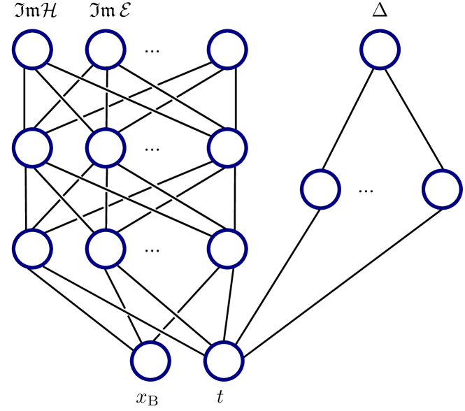
Figure 1: Architecture of neural nets when DR constraints are used. The main net parametrizes imaginary parts of CFFs, while the simpler subsidiary net parametrizes the subtraction constant $\Delta(t)$. Real parts are then obtained using DR (1). Observables are calculated using total complex CFFs, and, finally, differences with respect to measured observables are back-propagated for weight adjustment of the network neurons. There are also standard “bias” nodes which are for clarity not drawn. Architectures (number of neurons per layer, starting from the input layer) of our main nets are $[2\!\to\!13\!\to\!6]$ (for model NN20), $[2\!\to\!13\!\to\!4]$ (NNDR20), and $[2\!\to\!11\!\to\!17\!\to\!8]$ (fNNDR20), while subtraction constant nets are $[1\!\to\!3\!\to\!1]$ (unflavored), $[1\!\to\!5\!\to\!1]$ ($u$-quark), and $[1\!\to\!4\!\to\!1]$ ($d$-quark).

First, to assess the influence of DR, we made fits to the proton-only DVCS data using two parametrizations

1. using neural network parametrization of four imaginary parts of CFFs and of $\operatorname{\mathfrak{Re}}{\mathcal{H}}$ and $\operatorname{\mathfrak{Re}}{\mathcal{E}}$ (i.e. without imposing DR constraints) — this gives us the model NN20.

2. using neural network parametrization of four imaginary parts of CFFs, and of the subtraction constant, while $\operatorname{\mathfrak{Re}}{\mathcal{H}}$ and $\operatorname{\mathfrak{Re}}{\mathcal{E}}$ are then given by DR (1) — this gives us the model NNDR20.

After we convinced ourselves that the DR-constrained neural net parametrization works in the proton-only case, we made a separate parametrization for two light quark flavours (essentially doubling everything) and fitted to the combined proton and neutron DVCS data — this gave us the model fNNDR20.

II.3 Experimental data used

Table 1: Values of $\chi^{2}/n_{\mathrm{pts}}$ for presented models and for each set of DVCS measurements with fixed proton or neutron target used in this study ($\phi$-space). First row specifies the number of real independent CFFs plus the number of subtraction constants. Second row gives total value for all datapoints in actually performed fit (which was just to leading harmonics of Fourier-transformed data — $n$-space).

Observable	$n_{\mathrm{pts}}$	KM20	NN20	NNDR20	fKM20	fNNDR20
# CFFs + $\Delta$s		3+1	6	4+1	5+2	8+2
Total (harmonics)	277	1.3	1.6	1.7	1.7	1.8
CLAS Pisano et al. (2015) $A_{\rm LU}$	162	0.9	1.0	1.1	1.2	1.3
CLAS Pisano et al. (2015) $A_{\rm UL}$	160	1.5	1.7	1.8	1.8	2.0
CLAS Pisano et al. (2015) $A_{\rm LL}$	166	1.3	3.9	0.8	1.1	1.6
CLAS Jo et al. (2015) $d\sigma$	1014	1.1	1.0	1.2	1.2	1.1
CLAS Jo et al. (2015) $\Delta\sigma$	1012	0.9	0.9	1.0	0.9	1.1
Hall A Defurne et al. (2015) $d\sigma$	240	1.2	1.9	1.7	0.9	1.3
Hall A Defurne et al. (2015) $\Delta\sigma$	358	0.7	0.8	0.8	0.7	0.7
Hall A Defurne et al. (2017) $d\sigma$	450	1.5	1.6	1.7	1.9	2.0
Hall A Defurne et al. (2017) $\Delta\sigma$	360	1.6	2.2	2.2	1.9	1.7
Hall A Benali et al. (2020) $d\sigma_{n}$	96				1.2	0.9
Total ($\phi$-space)	4018	1.1	1.3	1.3	1.2	1.3

For the neural network fits we used the JLab DVCS data listed in Table 1. We excluded the lower-$x$ HERA data because we wanted to be safe from any $Q^{2}$ evolution effects since QCD evolution is not yet implemented in our neural network framework. Also, in order to demonstrate flavor separation, it made sense to restrict ourselves to the particular kinematic region where the neutron DVCS measurement was performed such that there is some balance between the proton and neutron data.

The data contains measurements of the unpolarized cross-section $d\sigma$, various beam and target asymmetries defined via

$$d\sigma_{\lambda,\Lambda}=d\sigma(1+\lambda A_{LU}+\Lambda A_{UL}+\lambda\Lambda A_{LL})\;,$$ (5)

as well as the helicity-dependent cross-section $\Delta\sigma\equiv d\sigma A_{LU}$. Furthermore, since leading-twist formulae Belitsky et al. (2002); Belitsky and Müller (2010) describe observables as truncated Fourier series in $\phi$, with only one or two terms, we made a Fourier transform of the data, and fitted only to these first harmonics. This makes the fitting procedure much more efficient. We propagated the experimental uncertainties using the Monte-Carlo method, and checked that, indeed, no harmonics beyond the second one are visible in the data with any statistical significance.

III Results and conclusion

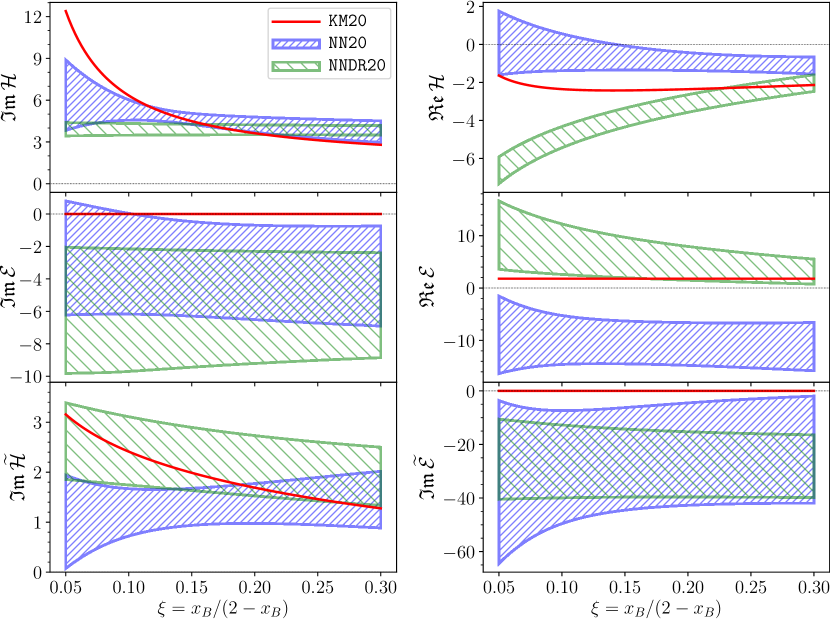
Figure 2: Extraction of CFFs (at $Q^{2}=4\,^{2}$ and $t=-0.2\,^{2}$) by three fits to JLab proton DVCS data. KM20 is model described in Sect. II.1, NN20 is standard neural network parametrization, while NNDR20 additionally includes DR constraints. $\operatorname{\mathfrak{Im}}{\mathcal{E}}$ and $\operatorname{\mathfrak{Im}}{\widetilde{\mathcal{E}}}$ are zero in KM20 model by construction.

The quality of the fit for each model is displayed in Table 1. Judging this quality by the $\chi^{2}$ values for fits of the above-mentioned Fourier harmonics of the data (second row of Table 1) is problematic, because propagation of experimental uncertainties to subleading harmonics is impaired by unknown correlations, see discussion in Sect. 3.1 of Kumerički et al. (2016). We consider the values of $\chi^{2}$ for the published experimental $\phi$-dependent data as a better measure of the actual fit quality. These are displayed in other rows of Table 1. Some particular datasets are imperfectly described, but total values of $\chi^{2}/n_{\rm pts}$ of 1.1–1.3 look reasonable and give us confidence that the resulting CFFs are realistic. Note that the significantly different number of independent CFFs in our models (see the first row of Table 1) leads to a similar quality of fits. One concludes that there are some correlations among CFFs. Some are intrinsic, like the consequence of DR, while some will be broken with more data, on more observables.

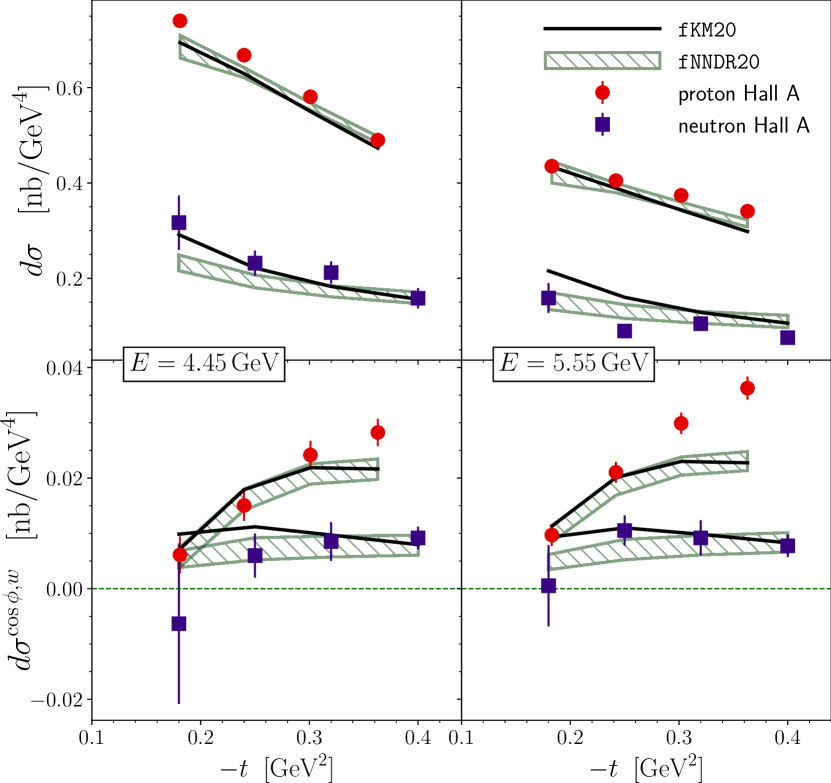
Figure 3: Model fit fKM20 (black solid line) and neural network fit fNNDR20 (hatched green band) in comparison to Hall A DVCS data on proton (red circles) and neutron (blue squares) cross-sections (upper two panels) and first cosine Fourier harmonics of cross-sections (lower two panels), for $x_{B}=0.36$, $Q^{2}=1.75\,^{2}$, and two beam energies, $E=4.45\,$ (left) and $E=5.55\,$ (right).

On Fig. 2 we display CFFs for models KM20, NN20 and NNDR20 obtained from fits to proton-only data. We observe the power of DR constraints, which lead to reduced uncertainties of the NNDR20 model in comparison to NN20, most notably for $\operatorname{\mathfrak{Im}}{\mathcal{H}}$, $\operatorname{\mathfrak{Re}}{\mathcal{H}}$, and $\operatorname{\mathfrak{Im}}{\widetilde{\mathcal{E}}}$. Mean values are also shifted for real parts of unpolarized CFFs $\mathcal{H}$ and $\mathcal{E}$, where DR constraints can even change the sign of the extracted CFFs. For $\operatorname{\mathfrak{Re}}{\mathcal{H}}$, DR induce a strong $\xi$ dependence and a clear extraction of this CFF. It is this particular effect of DR that made recent attempts at determination of quark pressure distribution in the proton from the DVCS data possible Burkert et al. (2018); Kumerički (2019). The DR-constrained neural net fit NNDR20 is, as is to be expected, in somewhat better agreement with the model fit KM20 which is also DR constrained. The green bands in the second row of Fig. 2 constitute the first unbiased extraction of the important CFF $\mathcal{E}$ in this kinematic region.

The CFFs in the NNDR20 model are in broad agreement with the results of the (also DR-constrained) model fit of Ref. Moutarde et al. (2018). One notable exception is the opposite sign of $\operatorname{\mathfrak{Im}}{\mathcal{E}}$. As this CFF has the largest uncertainty of the six displayed, one can hope that with more data the discrepancy will fade. Comparing with CFFs extracted by the recent global neural network fit of Ref. Moutarde et al. (2019), results agree within specified uncertainties, with the largest tension now being observed for $\operatorname{\mathfrak{Re}}{\mathcal{E}}$. One notes that $\operatorname{\mathfrak{Re}}{\mathcal{E}}$ of Moutarde et al. (2019) agrees much better with our fit NN20, which is to be expected since one is now comparing results of more similar procedures: both are completely unbiased fits, with neither using DR constraints.

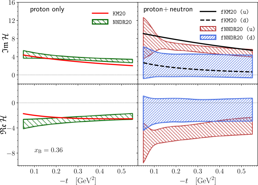
Figure 4: CFF $\mathcal{H}$ extracted (at $Q^{2}=4\,^{2}$ and $x_{\rm B}=0.36$) from neural network fit to proton-only DVCS data (left). Separation of $u$ (red band) and $d$ (blue band) quark CFF $\mathcal{H}$ resulting from neural network fit to proton and neutron JLab DVCS data (right). Red solid (unflavored), black solid ($u$) and dashed ($d$) lines correspond to analogous least-squares model fit to the same data.

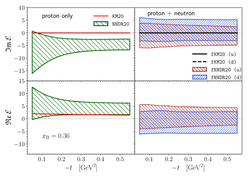
Figure 5: Same as Fig. 4 but for CFF $\mathcal{E}$. Separation of $u$ and $d$ quark CFF $\mathcal{E}$ is not possible with present data (right). $\operatorname{\mathfrak{Im}}{\mathcal{E}}$ is zero in KM models by construction.

Turning now to the simultaneous fit to proton and neutron data, besides in Table 1, the quality of the fit can also be seen in Fig. 3, where the model fit fKM20 and the DR-constrained neural net fit fNNDR20 are confronted with Hall A data. The resulting $\operatorname{\mathfrak{Im}}{\mathcal{H}}$ and $\operatorname{\mathfrak{Re}}{\mathcal{H}}$ CFFs, separately for up and down quarks, are displayed in the right two panels of Fig. 4, demonstrating how the inclusion of neutron DVCS data enables a clear flavor separation for this CFF. (For other CFFs, there is no visible separation, see example of $\mathcal{E}$ in Fig. 5.)

The separated up and down quark CFFs have much larger uncertainties than their sum, shown in the left panels of Fig. 4, and although there are some hints of different $t$-slopes, at this level we are not yet able to address the question of possible different spatial distributions of up and down quarks in the nucleon.

To conclude, we have used JLab DVCS data to make both a model-dependent and an unbiased neural net extraction of six Compton form factors, where constraints by dispersion relations proved valuable. Furthermore, in the case of the dominant CFF $\mathcal{H}$, we have successfully separated the contributions of up and down quarks. This constitutes another step towards a full three-dimensional picture of the nucleon structure.

Code availability

In the interest of open and reproducible research, the computer code used in the production of numerical results and plots for this paper is made available at https://github.com/openhep/neutron20.

Acknowledgments

This publication is supported by the Croatian Science Foundation project IP-2019-04-9709, by Deutsche Forschungsgemeinschaft (DFG) through the Research Unit FOR 2926, “Next Generation pQCD for Hadron Structure: Preparing for the EIC”, project number 40824754, by QuantiXLie Centre of Excellence through grant KK.01.1.1.01.0004, and the EU Horizon 2020 research and innovation programme, STRONG-2020 project, under grant agreement No 824093.

References

- Accardi et al. (2016) A. Accardi et al., Eur. Phys. J. A52, 268 (2016), eprint 1212.1701.
- Müller et al. (1994) D. Müller, D. Robaschik, B. Geyer, F. M. Dittes, and J. Hořejší, Fortschr. Phys. 42, 101 (1994), eprint hep-ph/9812448.
- Radyushkin (1996) A. V. Radyushkin, Phys. Lett. B380, 417 (1996), eprint hep-ph/9604317.
- Ji (1997) X.-D. Ji, Phys. Rev. D55, 7114 (1997), eprint hep-ph/9609381.
- Burkardt (2000) M. Burkardt, Phys. Rev. D62, 071503 (2000), erratum-ibid.D66:119903,2002, eprint hep-ph/0005108.
- d’Hose et al. (2016) N. d’Hose, S. Niccolai, and A. Rostomyan, Eur. Phys. J. A52, 151 (2016).
- Kumerički et al. (2016) K. Kumerički, S. Liuti, and H. Moutarde, Eur. Phys. J. A52, 157 (2016), eprint 1602.02763.
- Benali et al. (2020) M. Benali et al., Nature Phys. 16, 191 (2020).
- Belitsky et al. (2002) A. V. Belitsky, D. Müller, and A. Kirchner, Nucl. Phys. B629, 323 (2002), eprint hep-ph/0112108.
- Belitsky and Müller (2010) A. V. Belitsky and D. Müller, Phys.Rev. D82, 074010 (2010), eprint 1005.5209.
- Teryaev (2005) O. V. Teryaev (2005), eprint hep-ph/0510031.
- Kumerički and Müller (2010) K. Kumerički and D. Müller, Nucl. Phys. B841, 1 (2010), eprint 0904.0458.
- Kumerički and Müller (2016) K. Kumerički and D. Müller, EPJ Web Conf. 112, 01012 (2016), eprint 1512.09014.
- Kumerički et al. (2011) K. Kumerički, D. Müller, and A. Schäfer, JHEP 07, 073 (2011), eprint 1106.2808.
- Forte et al. (2002) S. Forte, L. Garrido, J. I. Latorre, and A. Piccione, JHEP 05, 062 (2002), eprint hep-ph/0204232.
- Schaul et al. (2010) T. Schaul, J. Bayer, D. Wierstra, Y. Sun, M. Felder, F. Sehnke, T. Rückstieß, and J. Schmidhuber, The Journal of Machine Learning Research 11, 743 (2010).
- Kumerički (2019) K. Kumerički, Nature 570, E1 (2019).
- Moutarde et al. (2019) H. Moutarde, P. Sznajder, and J. Wagner, Eur. Phys. J. C79, 614 (2019), eprint 1905.02089.
- Pisano et al. (2015) S. Pisano et al. (CLAS) (2015), eprint 1501.07052.
- Jo et al. (2015) H. Jo et al. (CLAS), Phys. Rev. Lett. 115, 212003 (2015), eprint 1504.02009.
- Defurne et al. (2015) M. Defurne et al. (Hall A), Phys. Rev. C92, 055202 (2015), eprint 1504.05453.
- Defurne et al. (2017) M. Defurne et al., Nature Commun. 8, 1408 (2017), eprint 1703.09442.
- Vanderhaeghen et al. (1999) M. Vanderhaeghen, P. A. M. Guichon, and M. Guidal, Phys. Rev. D60, 094017 (1999), eprint hep-ph/9905372.
- Goloskokov and Kroll (2008) S. V. Goloskokov and P. Kroll, Eur.Phys.J. C53, 367 (2008), eprint 0708.3569.
- Moutarde et al. (2018) H. Moutarde, P. Sznajder, and J. Wagner, Eur. Phys. J. C78, 890 (2018), eprint 1807.07620.
- Burkert et al. (2018) V. D. Burkert, L. Elouadrhiri, and F. X. Girod, Nature 557, 396 (2018).