Ideal formulations for constrained convex optimization problems with indicator variables

Abstract

Motivated by modern regression applications, in this paper, we study the convexification of a class of convex optimization problems with indicator variables and combinatorial constraints on the indicators. Unlike most of the previous work on convexification of sparse regression problems, we simultaneously consider the nonlinear non-separable objective, indicator variables, and combinatorial constraints. Specifically, we give the convex hull description of the epigraph of the composition of a one-dimensional convex function and an affine function under arbitrary combinatorial constraints. As special cases of this result, we derive ideal convexifications for problems with hierarchy, multi-collinearity, and sparsity constraints. Moreover, we also give a short proof that for a separable objective function, the perspective reformulation is ideal independent from the constraints of the problem. Our computational experiments with sparse regression problems demonstrate the potential of the proposed approach in improving the relaxation quality without significant computational overhead.

Keywords: Convexification, perspective formulation, Indicator variables, combinatorial constraints.

1 Introduction

Given a set $Q\subseteq\{0,1\}^{p}$, a vector $h\in\mathbb{R}^{p}$ such that $h_{i}\neq 0$, for all $i\in[p]{\color[rgb]{0,0,0}{:=\left\{1,\ldots,p\right\}}}$, and a convex function $f:\mathbb{R}\to\mathbb{R}$, we study the set

$$Z_{Q}=\left\{(z,\beta,t)\in Q\times\mathbb{R}^{p}\times\mathbb{R}~{}|~{}f\left(h^{\top}\beta\right)\leq t,\beta_{i}(1-z_{i})=0,\forall i\in[p]\right\}.$$

In set $Z_{Q}$ above, $z$ is a vector of indicator variables with $z_{i}=1$ if $\beta_{i}\neq 0$, and the set $Q$ encodes combinatorial constraints on the indicator variables. We assume without loss of generality that $f(0)=0$, since this assumption can always be satisfied after subtracting the constant term $f(0)$.

The motivation to study $Z_{Q}$ stems from sparse regression problem: Given a set of observations $(x_{i},y_{i})_{i=1}^{n}$ where $x_{i}\in\mathbb{R}^{p}$ are the features corresponding to observation $i$ and $y_{i}\in\mathbb{R}$ is its associated response variable, inference with a sparse linear model can be modeled as the optimization problem

$$\min_{z,\beta}\; \sum_{i=1}^{n}f\left(y_{i},x_{i}^{\top}\beta\right)+\lambda\rho(\beta)$$ (1a)

s.t. $$\beta_{i}(1-z_{i})=0, i\in[p]$$ (1b)

$$\beta\in\mathbb{R}^{p},\;z\in Q\subseteq\{0,1\}^{p},$$ (1c)

where $\beta$ is a vector of regression coefficients, $f$ is a loss function, $\lambda\geq 0$ is a regularization parameter and $\rho$ is regularization function. Often, $f(\beta)=\left(y_{i}-x_{i}^{\top}\beta\right)^{2}$, in which case (1) is referred to as sparse least squares regression, and typical choices of $\rho$ include $\ell_{0}$, $\ell_{1}$, or $\ell_{2}$ regularizations.

If $Q$ is defined via a $q$-sparsity constraint, $Q=\left\{z\in\{0,1\}^{p}~{}|~{}\sum_{i=1}^{p}z_{i}\leq q\right\}$, then problem (1) reduces to the best subset selection problem [48], a fundamental problem in statistics. Nonetheless, constraints other than the cardinality constraint arise in several statistical problems. Bertsimas and King, [10] suggest imposing constraints of the form $\sum_{i\in S}z_{i}\leq 1$ for some $S\subseteq[p]$ to prevent multicollinearity; Carrizosa et al., [18] use similar constraints to capture nested categorical variables. Constraints of the form $z_{i}\leq z_{j}$ can be used to impose strong hierarchy relationships, and constraints of the form $z_{i}\leq\sum_{j\in H\subseteq[p]}z_{j}$ can be used for weak hierarchy relationships [14]. In group variable selection, indicator variables of regression coefficients of variables in the same group are linked, see [43]. Manzour et al., [47] and Küçükyavuz et al., [46] impose that the indicator variables, which correspond to edges in an underlying graph, do not define cycles—a necessary constraint for inference problems with causal graphs. Cozad et al., [21] suggest imposing a variety of constraints in both the continuous and discrete variables to enforce priors from human experts.

Problem (1) is $\mathcal{NP}$-hard even for a $q$-sparsity constraint [50], and is often approximated with a convex surrogate such as lasso [39, 55]. Solutions with better statistical properties than lasso can be obtained from non-convex continuous approximations [29, 63]. Alternatively, it is possible to solve (1) to optimality via branch-and-bound methods [11, 20]. In all cases, most of the approaches for (1) have focused on the $q$-sparsity constraint (or its Lagrangian relaxation). For example, a standard technique to improve the relaxations of (1) revolves around the use of the perspective reformulation [1, 19, 54, 27, 26, 31, 32, 34, 30, 36, 42, 61, 64], an ideal formulation of a separable quadratic function with indicators (but no additional constraints). Recent work on obtaining ideal formulations for non-separable quadratic functions [4, 6, 5, 27, 35, 44] also ignores additional constraints in $Q$.

There is a recent research thrust on studying constrained versions of (1). Dong et al., [25] study problem (1) from a continuous optimization perspective (after projecting out the discrete variables), see also [24]. Hazimeh and Mazumder, [40] give specialized algorithms for the natural convex relaxation of (1) where $Q$ is defined via strong hierarchy constraints. Several results exist concerning the convexification of nonlinear optimization problems with constraints [3, 8, 15, 17, 49, 52, 56, 45, 58, 59, 57, 16], but such methods in general do not deliver ideal, compact or closed-form formulations for the specific case of problem (1) with structured feasible regions. In a recent work closely related to the setting considered here, Xie and Deng, [62] prove that the perspective formulation is ideal if the objective is quadratic and separable, and $Q$ is defined by a $q$-sparsity constraint. In a similar vein, Bacci et al., [7] show that the perspective reformulations for convex differentiable functions are tight for 1-sum compositions, and they use this result to show that they are ideal under unit commitment constraints. However, similar results for more general (non-separable) objective functions or constraints are currently not known.

Our contributions. In this paper, we provide a first study (from a convexification perspective) of the interplay between non-separable convex objectives and combinatorial constraints on the indicator variables. Specifically, we derive the convex hull description of $Z_{Q}$: the result is stated in terms of the convexification of the combinatorial set $Q$, but places no assumptions on its form. Using this result, we develop ideal formulations for settings in which the logical constraints on the indicator variables encode sparsity constraints or the so-called strong and weak hierarchy relations. In addition, we generalize the result in [62] and [7] to arbitrary constraints on $z$ for separable convex functions $f$, in our setting. We show the computational benefit of the proposed approach on constrained regression problems with hierarchical relations.

An earlier version of this work appeared in [60], where we only considered separable and rank-one convex quadratic functions, and sparsity and strong hierarchy constraints. Furthermore, in [60], our proofs of the convexification results use the structure of each of the sets considered, whereas in the present paper, we give a unifying technique that generalizes to any combinatorial set for functions that are not necessarily quadratic. Finally, here, we expand on our preliminary computational experiments in [60] with additional datasets, conduct a further analysis on the choices of the regularization parameters, and perform computations with sparse logistic regression.

Notation. Given a one-dimensional convex function $f:\mathbb{R}\to\mathbb{R}$, we adopt the convention that $0f(\beta/0)=\lim_{z\to 0^{+}}zf(\beta/z)$. Using this convention, the function $zf(\beta/z)$ for $z\geq 0$ is the closure of the perspective function of $f$, and is convex. Let $\mathbf{0}$ and $\mathbf{1}$ be vectors of conformable dimension with all zeros and ones, respectively, and let $e_{i}$ denote the $i$th unit vector of appropriate dimension with 1 in the $i$th component and zeros elsewhere. For a set $Q$, we denote by $\text{conv}(Q)$ its convex hull and by $\operatorname{cl\ conv}(Q)$ the closure of its convex hull. Given two vectors $u,v$ of same dimensions, we let $u\circ v$ denote the Hadamard vector of $u$ and $v$, i.e., $(u\circ v)_{i}=u_{i}v_{i}$.

2 Convexification of $Z_{Q}$

Observe that in set $Z_{Q}$, the coefficients of $\beta$ can be scaled and negated if necessary to ensure $h_{i}=1$ for all $i\in[p]$. Therefore, in the derivation of ideal formulations in this section, we assume, without loss of generality, that

$$Z_{Q}=\left\{(z,\beta,t)\in Q\times\mathbb{R}^{p}\times\mathbb{R}~{}|~{}f\left(\mathbf{1}^{\top}\beta\right)\leq t,\beta_{i}(1-z_{i})=0,\forall i\in[p]\right\}.$$

We also assume, without loss of generality, that for every $i\in[p]$ there exists $z\in Q$ such that $z_{i}=1$, as otherwise $z_{i}=\beta_{i}=0$ can be fixed and the corresponding variables can be removed.

For a given set $Q$, let $Q^{0}=Q\setminus\{\mathbf{0}\}$ or, equivalently, $Q^{0}=\{z\in Q~{}|~{}\sum_{i=1}^{p}z_{i}\geq 1\}$. As we show in the subsequent discussion, the convexification of the set $Z_{Q}$ relies on the characterization of $\text{conv}(Q^{0})$. To this end, we first establish such a characterization.

Proposition 1.

The convex hull of $Q^{0}$ admits a description as

$$\text{conv}(Q^{0})=\text{conv}(Q)\bigcap\{z\;|\;\pi^{\top}z\geq 1,\;\forall\pi\in\mathcal{F}\},$$ (2)

where $\mathcal{F}$ is a finite subset of $\mathbb{R}^{p}$.

Proof.

Let $\pi^{\top}z\geq\pi_{0}$ be an arbitrary valid inequality for $\text{conv}(Q^{0})$. If $\pi_{0}>0$, then $\frac{1}{\pi_{0}}\pi^{\top}z\geq 1$ is an equivalent inequality satisfying the conditions in (2). Otherwise, if $\pi_{0}\leq 0$, then the inequality does not cut off $\mathbf{0}$ and is thus valid for $Q$ and $\text{conv}(Q)$. Therefore, it follows that $\text{conv}(Q)\subseteq\{z\;|\;\pi^{\top}z\geq\pi_{0}\}$, and inequality $\pi^{\top}z\geq\pi_{0}$ is either already a facet of $\text{conv}(Q)$, or is implied by the facets $\text{conv}(Q)$. Finally, finiteness of $\mathcal{F}$ follows since $\text{conv}(Q^{0})$ is a polyhedron.  ∎

Note that if $\mathbf{0}\not\in Q$, then $\mathcal{F}=\emptyset$. In practice, a set $\mathcal{F}$ of minimal cardinality is preferred. Since $\text{conv}(Q)$ and $\text{conv}(Q_{0})$ may have an exponential number of facets, set $\mathcal{F}$ may be exponentially large as well. In such cases, inequalities from $\mathcal{F}$ can be generated if violated in an iterative fashion, as is standard in a cutting plane algorithm. Note that even if $\text{conv}(Q)$ is simple, $\text{conv}(Q_{0})$ may contain an exponential number of facets. Nonetheless, in such cases, $\text{conv}(Q_{0})$ admits a compact extended formulation [2], which in turn implies that separation of the inequalities in $\mathcal{F}$ can be done in polynomial time.

Intuitively, one may think of $\mathcal{F}$ as the set of “new” facets of $\text{conv}(Q^{0})$ that are not facets of $\text{conv}(Q)$. If $\text{conv}(Q)$ and $\text{conv}(Q^{0})$ have the same dimension, this intuition is correct. However, if the dimension of $\text{conv}(Q^{0})$ is less than the dimension of $\text{conv}(Q)$, it may be the case that $\text{conv}(Q^{0})\subseteq\{z:\pi^{\top}z=1\}$ for some $\pi\in\mathcal{F}$, and thus this inequality is not a facet. For example, if $Q=\{0,1\}$, then $\text{conv}(Q)=[0,1]$, $Q^{0}=\text{conv}(Q^{0})=\{1\}$ and $\mathcal{F}=\{1\}$, but the inequality $z\geq 1$ is not a facet of the 0-dimensional polyhedron $\text{conv}(Q^{0})$.

The description of $\operatorname{cl\ conv}(Z_{Q})$ depends on the structure of $Q$, and is critically dependent on whether the variables can be partitioned into multiple mutually exclusive components. We formalize this characteristic next.

Definition 1.

For $i,j\in[p],i\neq j$, define $i\sim j$ if there exists some $z\in Q$ such that $z_{i}=z_{j}=1$. Define the graph $G_{Q}=(V,E)$ where $V=[p]$ and $\{i,j\}\in E$ if and only if $i\sim j$.

2.1 The connected case

In this section, we provide ideal formulations in the original space of variables when graph $G_{Q}$ in Definition 1 is connected. This assumption is satisfied in most of the practical applications we consider, see §3. Later, in §2.2, we build upon the results of this section to derive ideal formulations when $G_{Q}$ is not necessarily connected.

Before we propose a class of valid inequalities for $Z_{Q}$, we give a lemma.

Lemma 1.

For a one-dimensional proper convex function $f:\mathbb{R}\rightarrow\mathbb{R}$ with effective domain $\operatorname{dom}(f)=\mathbb{R}$, $f(0)=0$ and its perspective $g(x,t)=tf(\frac{x}{t})\;:\mathbb{R}^{2}\rightarrow\mathbb{R}$, if $0<t_{1}\leq t_{2}$, then $g(x,t_{1})\geq g(x,t_{2})$ for all $x\in\mathbb{R}$.

Proof.

It suffices to show that the function $\phi(x)=g(x,t_{1})-g(x,t_{2})$ is non-decreasing in $[0,+\infty]$ and non-increasing in $[-\infty,0]$. Since $\operatorname{dom}(f)=\mathbb{R}$, $f$ is continuous over $\mathbb{R}$ so is $\phi(x)$. Also, by convexity, we know that the right-derivative of $f(x)$ exists and is non-decreasing. Thus, $\phi_{+}^{{}^{\prime}}(x)=f_{+}^{{}^{\prime}}(\frac{x}{t_{1}})-f_{+}^{{}^{\prime}}(\frac{x}{t_{2}})\geq 0$ for all $x\in[0,+\infty]$. A continuous function with non-negative right-derivative is non-decreasing [38]. For $x\in[-\infty,0]$, the left-derivative of $\phi$ is $\phi_{-}^{{}^{\prime}}(x)=f_{-}^{{}^{\prime}}(\frac{x}{t_{1}})-f_{-}^{{}^{\prime}}(\frac{x}{t_{2}})\leq 0$, and similarly, $\phi(x)$ is non-increasing in $[-\infty,0]$.

∎

Proposition 2.

The inequalities

$$t\geq(\pi^{\top}z)f\left(\frac{\mathbf{1}^{\top}\beta}{\pi^{\top}z}\right),\;\;\forall\pi\in\mathcal{F}$$ (3)

are valid for $Z_{Q}$ for any finite set $\mathcal{F}\subseteq\mathbb{R}^{p}$ satisfying (2).

Proof.

First, observe that if $\mathbf{0}\not\in Q$, then $\mathcal{F}=\emptyset$ and the statement is superfluous. Suppose, $\mathcal{F}\neq\emptyset.$ We consider two cases. If $z\neq\mathbf{0}$, then we have $\pi^{\top}z\geq 1$ for $\pi\in\mathcal{F}$. Then, from Lemma 1, $(\pi^{\top}z)f\left(\frac{\mathbf{1}^{\top}\beta}{\pi^{\top}z}\right)\leq f\left(\mathbf{1}^{\top}\beta\right)\leq t$. Hence the inequality is valid. Finally, if $z=\mathbf{0}$, then $\beta=\mathbf{0}$ in $Z_{Q}$. Therefore,

$$t\geq f\left(\mathbf{1}^{\top}\beta\right)=f(0)=0=\lim_{\zeta\to 0^{+}}\zeta f\left(0/\zeta\right)=(\pi^{\top}z)f\left(\frac{\mathbf{1}^{\top}\beta}{\pi^{\top}z}\right),$$

and the inequality is valid. ∎

We now describe the closure of the convex hull of $Z_{Q}$ under the assumption that graph $G_{Q}$ described in Definition 1 is connected.

Theorem 1.

If the graph $G_{Q}$ given in Definition 1 is connected, then

$$\operatorname{cl\ conv}(Z_{Q})=\Big{\{}(z,\beta,t)\in[0,1]^{p}\times\mathbb{R}^{p} \times\mathbb{R}\;|\;z\in\text{conv}(Q),\;t\geq f(\mathbf{1}^{\top}\beta),$$

$$t\geq(\pi^{\top}z)f\left(\frac{\mathbf{1}^{\top}\beta}{\pi^{\top}z}\right),\;\;\forall\pi\in\mathcal{F}\Big{\}}$$ (4)

for any finite set $\mathcal{F}\subseteq\mathbb{R}^{p}$ satisfying (2).

Note that if $\mathbf{0}\not\in Q$, i.e., $\mathcal{F}=\emptyset$, then Theorem 1 states that the description of $\operatorname{cl\ conv}(Z_{Q})$ is obtained simply by dropping the complementarity constraints $\beta_{i}(1-z_{i})=0,\forall i\in[p]$ and independently taking the convex hull of $Q$. Otherwise, since the description of $\operatorname{cl\ conv}(Z_{Q})$ requires a new inequality for every element of $\mathcal{F}$, a minimal description of $\mathcal{F}$ is certainly preferred from a computational standpoint. If $\text{conv}(Q^{0})$ is full-dimensional, the strongest nonlinear inequalities (3) are obtained from facets of $\text{conv}(Q^{0})$. Moreover, in many situations, it may not be possible to have a full description of $\text{conv}(Q)$ or $\text{conv}(Q^{0})$; nonetheless, in those cases, it may be possible to obtain a facet $\bar{\pi}^{\top}x\geq 1$ of $\text{conv}(Q^{0})$, and Theorem 1 ascertains that the valid inequality

$$t\geq(\bar{\pi}^{\top}z)f\left(\frac{\mathbf{1}^{\top}\beta}{\bar{\pi}^{\top}z}\right)$$ (5)

is not dominated by any other inequality of a similar form, and that inequalities of this form are sufficient to describe $\operatorname{cl\ conv}(Z_{Q})$. In Appendix A we focus on the special case where $\text{conv}(Q)$ admits a compact representation but $\text{conv}(Q_{0})$ has exponentially many inequalities: We show how to use a compact extended formulation of $\text{conv}(Q_{0})$ to derive the description of $\operatorname{cl\ conv}(Z_{Q})$ in a higher dimensional space.

Before proving Theorem 1, we give a lemma used in the proof.

Lemma 2.

$z\in\text{conv}(Q)$ if and only if there exists some $\alpha\in[0,1]$ and $z^{0}\in\text{conv}(Q^{0})$ such that $z=\alpha z^{0}$.

Proof.

Note that if $\mathbf{0}\not\in Q$, then the result holds trivially by letting $\alpha=1$. Therefore, we will assume that $\mathbf{0}\in Q$.

($\Rightarrow$) Let $z\in\text{conv}(Q)$. So we can write $z$ as a convex combination of the extreme points of $Q$. Specifically, we distinguish between the feasible points $z^{i}\in Q^{0}$ for $i\in\mathcal{I}$ and the origin. In particular, there exists $\gamma\geq\mathbf{0}$ with $\sum_{i\in\mathcal{I}\cup\{0\}}\gamma_{i}=1$, such that

$$z =\gamma_{0}\mathbf{0}+\sum_{i\in\mathcal{I}}\gamma_{i}z^{i}=\left(\sum_{i\in\mathcal{I}}\gamma_{i}\right)\sum_{i\in\mathcal{I}}\frac{\gamma_{i}}{\sum_{i\in\mathcal{I}}\gamma_{i}}z^{i}.$$

Letting $\alpha=\sum_{i\in\mathcal{I}}\gamma_{i}$, the result follows.

($\Leftarrow$) Let $z=\alpha z^{0}$ for some $\alpha\in[0,1]$ and $z^{0}\in\text{conv}(Q^{0})$; by definition, we can expand $z^{0}$ as $z^{0}=\sum_{i\in\mathcal{I}}\gamma_{i}z^{i}$, a convex combination of $z^{i}\in Q^{0}$. By adding the term $(1-\alpha)\mathbf{0}$, we have $z=(1-\alpha)\mathbf{0}+\sum_{i\in\mathcal{I}}\alpha\gamma_{i}z^{i}$.  ∎

We are now ready to prove Theorem 1.

Proof of Theorem 1.

Define $Y$ as the set described by (4). Let $a,b\in\mathbb{R}^{p},c\in\mathbb{R}$, and consider the two optimization problems

$$\min_{z,\beta,t}\; a^{\top}z+b^{\top}\beta+ct\quad\text{subject to}\quad(z,\beta,t)\in Z_{Q},\text{ and}$$ (6)

$$\min_{z,\beta,t}\; a^{\top}z+b^{\top}\beta+ct\quad\text{subject to}\quad(z,\beta,t)\in Y.$$ (7)

We show that there exists a solution $(z,\beta,t)$ optimal for both problems, and that the corresponding objective values of both problems coincide.

$\bullet$ Simple cases:

If $c<0$, then both (6) and (7) are unbounded. To see this, let $z=\beta=\mathbf{0}$, and $t=\kappa$, where $\kappa\geq 0$. This solution is feasible for both (6) and (7). Letting $\kappa\to\infty$, the objective goes to minus infinity.

If $c=0$ and $b\neq\mathbf{0}$, then let $z_{j}=1$ for some $j\in[p]$ such that $b_{j}\neq 0$, and let $\beta_{j}$ go to plus or minus infinity depending on whether $b_{j}$ is negative or positive, respectively, while keeping $\beta_{i}=0$ for $i\neq j$. Again, the objective goes to minus infinity.

If $c=0$ and $b=\mathbf{0}$, then these two problems reduce to minimizing $a^{\top}z$ over $\text{conv}(Q)$ and thus (6) and (7) are equivalent.

If $c>0$, then we assume, without loss of generality, that $c=1$ by scaling. If there exists $i_{0}\neq j_{0}$ such that $b_{i_{0}}\neq b_{j_{0}}$, then there exists some $i$ and $j$ in a path from $i_{0}$ and $j_{0}$ in $G_{Q}$ such that $i\sim j$ and $b_{i}\neq b_{j}$, and without loss of generality, we assume $b_{i}<b_{j}$. Furthermore, there exists some $z\in Q$ such that $z_{i}=z_{j}=1$. Then we take such a vector $z$, we let $\beta$ be a vector of zeros except for $\beta_{i}=-\beta_{j}=\kappa$ for some $\kappa>0$, and we let $t=f(\mathbf{1}^{\top}\beta)=0$. Such a triplet $(z,\beta,t)$ is in $Z_{Q}$ and $Y$, and by letting $\kappa\to\infty$, the objective goes to minus infinity. Therefore, we assume in the sequel that $b_{i}=\bar{b}$ for all $i\in[p]$.

$\bullet$ Case $c=1$ and $b=\bar{b}\mathbf{1}$:

We now show that for $b=\bar{b}\mathbf{1}$ problem (7) either has a finite optimal solution that is in set $Z_{Q}$ or is unbounded. Note that (7) is equivalent to:

$$\min_{z,\beta}\quad a^{\top}z+\bar{b}\left(\mathbf{1}^{\top}\beta\right)+\max\left\{f\left(\mathbf{1}^{\top}\beta\right),\max_{\pi\in\mathcal{F}}\left\{\left(\pi^{\top}z\right)f\left(\frac{\mathbf{1}^{\top}\beta}{\pi^{\top}z}\right)\right\}\right\}$$

s.t. $$z\in\text{conv}(Q),$$

and, from Lemma 1, it further simplifies to

$$\min_{z,\beta}\quad a^{\top}z+\bar{b}\left(\mathbf{1}^{\top}\beta\right)+\min_{\pi\in\mathcal{F}}\{\pi^{\top}z,1\}f\left(\frac{\mathbf{1}^{\top}\beta}{\min_{\pi\in\mathcal{F}}\{\pi^{\top}z,1\}}\right)$$ (8a)

s.t. $$z\in\text{conv}(Q).$$ (8b)

Let $f^{*}:\mathbb{R}\to\mathbb{R}$ be the convex conjugate of function $f$, i.e., $f^{*}(\gamma)=\sup_{x\in\mathbb{R}}\gamma x-f(x)$, and let $\Gamma=\left\{\gamma\in\mathbb{R}:f^{*}(\gamma)<\infty\right\}$ be the domain of $f^{*}$. Note that if $-\bar{b}\not\in\Gamma$, it follows that both (6) and (7) are unbounded. Thus, we assume in the sequel that $-\bar{b}\in\Gamma$.

Observe that, given $w>0$, the convex conjugate of the function $wf(x/w)$ is $wf^{*}(\gamma)$. Hence, from Fenchel inequality, we find that, for any $\beta$, $z$ such that $\pi^{\top}z>0$, and $\gamma\in\Gamma$,

$$\min_{\pi\in\mathcal{F}}\{\pi^{\top}z,1\}f\left(\frac{\mathbf{1}^{\top}\beta}{\min_{\pi\in\mathcal{F}}\{\pi^{\top}z,1\}}\right)\geq\gamma(\mathbf{1}^{\top}\beta)-\min_{\pi\in\mathcal{F}}\{\pi^{\top}z,1\}f^{*}(\gamma).$$ (9)

Furthermore, for $\pi^{\top}z=0$ for some $\pi\in\mathcal{F}$, if the left hand side of (9) is infinity, then the inequality holds trivially; otherwise, if the left hand side of (9) is $0f((\mathbf{1}^{\top}\beta)/0)=\lim_{z\to 0^{+}}zf((\mathbf{1}^{\top}\beta)/z)=d$ with $|d|<\infty$, then by continuity of the functions at both sides of the inequality, (9) is satisfied.

Using (9) with $\gamma=-\bar{b}$ to lower bound the last term in (8a), we obtain the relaxation

$$\min_{z,\beta,t}\quad a^{\top}z+\bar{b}\left(\mathbf{1}^{\top}\beta\right)+\left(-\bar{b}(\mathbf{1}^{\top}\beta)-\min_{\pi\in\mathcal{F}}\{\pi^{\top}z,1\}f^{*}(-\bar{b})\right)$$

s.t. $$z\in\text{conv}(Q),$$

or, equivalently,

$$\min_{z}\quad a^{\top}z+\max_{\pi\in\mathcal{F}}\{1-\pi^{\top}z,0\}f^{*}(-\bar{b})-f^{*}(-\bar{b})$$ (10a)

s.t. $$z\in\text{conv}(Q).$$ (10b)

We will first prove that relaxation (10) admits an optimal solution integral in $z$, and then we will show that the lower bound from the relaxation is in fact tight.

Note that if $\mathbf{0}\not\in Q$, then $\mathcal{F}=\emptyset$ and there exists an optimal integer solution $z^{*}\in Q$ to the relaxation (10) with objective value $a^{\top}z^{*}-f^{*}(-\bar{b})$.

Now consider the case that $\mathbf{0}\in Q$. Let $z^{*}$ be an optimal solution of (10), and consider two subcases.

$\bullet$ Subcase (i):

First, suppose that $1-\pi^{\top}z^{*}\leq 0$ for all $\pi\in\mathcal{F}$. In this case, (10) is equivalent to

$$\min_{z}\quad\; a^{\top}z-f^{*}(-\bar{b})$$ (11a)

s.t. $$\pi^{\top}z\geq 1 \forall\pi\in\mathcal{F}$$ (11b)

$$z\in\text{conv}(Q).$$ (11c)

From Proposition 1, the feasible region of (11) is precisely $\text{conv}(Q^{0})$, thus problem (11) admits an optimal integer solution $z^{*}\in Q^{0}$ with objective value $a^{\top}z^{*}-f^{*}(-\bar{b})$.

$\bullet$ Subcase (ii):

Let $\bar{\pi}\in{\arg\min}_{\pi\in\mathcal{F}}\pi^{\top}z^{*}$, and suppose that $1-\bar{\pi}^{\top}z^{*}>0$. In this case, problem (10) is equivalent to

$$\ell=\min_{z}\quad a^{\top}z-(\bar{\pi}^{\top}z)f^{*}(-\bar{b})$$ (12a)

s.t. $$\pi^{\top}z\geq\bar{\pi}^{\top}z \forall\pi\in\mathcal{F}$$ (12b)

$$z\in\text{conv}(Q).$$ (12c)

Note that $f^{*}(-\bar{b})=\sup_{x\in\mathbb{R}}-\bar{b}x-f(x)\geq 0$, because $x=0$ is a possible solution to the supremum problem and $f(0)=0$. Since $z=\mathbf{0}$ is feasible for (12), we find that the objective value $\ell\leq 0$. If $\ell=0$, then $z^{*}=\mathbf{0}$ is optimal and the proof is complete. Suppose now that $\ell<0$. Observe from Lemma 2 that $z^{*}=\alpha z_{0}$ for some $z_{0}\in\text{conv}(Q^{0})$ and $\alpha\in(0,1)$—the case $\alpha=1$ is excluded, since $1-\bar{\pi}^{\top}z_{0}\leq 0$ for any $z_{0}\in\text{conv}(Q^{0})$. Consequently, the point $\bar{z}=z_{0}=\frac{z^{*}}{\alpha}$, with objective value $\bar{\ell}=\ell/\alpha<\ell$ is feasible for (12) with better objective value than $z^{*}$, resulting in a contradiction.

From subcases (i) and (ii), we see that either $z^{*}=\mathbf{0}$ is feasible and optimal for relaxation (10) (with objective value $0$), or that there exists an optimal integer solution $z^{*}$ with objective value $a^{\top}z^{*}-f^{*}(-\bar{b})$, regardless of whether $\mathbf{0}\in Q$ or not. We now prove that the lower bound provided by the relaxation (10) is tight, by finding $\beta^{*}\in\mathbb{R}^{p}$ such that $(z^{*},\beta^{*},f(\mathbf{1}^{\top}\beta^{*}))$ is feasible for (6) with the same objective value as (10). If $z^{*}=\mathbf{0}$, then clearly $(\mathbf{0},\mathbf{0},0)$ is optimal for (6) with objective value $0$, and we now focus on the case $z^{*}\neq\mathbf{0}$. Let $\bar{x}\in{\arg\sup}_{x\in\mathbb{R}}-\bar{b}x-f(x)$ and suppose that $\bar{x}$ exists, i.e., $\sup$ can be changed to $\max$, and observe that $f^{*}(-\bar{b})=-\bar{b}\bar{x}-f(\bar{x})$, or in other words

$$a^{\top}z-f^{*}(-\bar{b})=a^{\top}z+\bar{b}\bar{x}+f(\bar{x}).$$

Since $z^{*}\neq\mathbf{0}$, there exists $i$ such that $z_{i}^{*}=1$. Setting $\beta_{i}^{*}=\bar{x}$, $\beta_{j}^{*}=0$ for $j\neq i$, we find that the point $(z^{*},\beta^{*},f(\beta^{*}))$ is feasible for both (6) and (7), and since its objective value is the same as the lower bound obtained from (10), it is optimal for both problems. Now suppose that $\bar{x}$ above does not exist, but $(\bar{x}^{1},\bar{x}^{2},\ldots)$ is a sequence of points such that $-\bar{b}\bar{x}^{i}-f(\bar{x}^{i})\to f^{*}(-\bar{b})$. In this case, using identical arguments as above, we find a sequence of feasible points with objective value converging to $a^{\top}z^{*}-f^{*}(-\bar{b})$: thus, the latter corresponds to the infimum of (7) and the relaxation is tight. ∎

2.2 The general case

In this section, we give ideal formulations for $Z_{Q}$ when graph $G_{Q}$ in Definition 1 has several connected components. Given the graph $G_{Q}=(V,E)$, let $V_{1},V_{2},\dots,V_{k}$ be the vertex partition of connected components of $G_{Q}$. Let $\beta_{V_{\ell}}$ represent the subvector of $\beta$ corresponding to indices $V_{\ell}$. Then

$$\forall(z,\beta,t)\in Z_{Q},f(\mathbf{1}^{\top}\beta)=\sum_{\ell=1}^{k}f(\mathbf{1}^{\top}\beta_{V_{\ell}}),$$

because we cannot have two indices $i,j$ from different connected components such that $z_{i}=z_{j}=1$. In other words, if $\beta_{i}\neq 0$ for some $i\in V_{\ell},\ell\in[k]$, then $\beta_{j}=0$ for all $j\in[p]\backslash V_{\ell}$.

For any $\ell=1,\ldots,k$, define the projection of the binary set $Q$ onto $V_{\ell}$ as

$$Q_{\ell}=\{z\in\{0,1\}^{p}\;|\;z\in Q,z_{i}=0,\;\forall i\notin V_{\ell}\},$$

let $Q_{\ell}^{0}=Q_{\ell}\setminus\{\mathbf{0}\}$ and note that, using arguments identical to those of Proposition 1, each $\text{conv}(Q_{\ell}^{0})$ admits a description as

$$\text{conv}(Q_{\ell}^{0})=\text{conv}(Q_{\ell})\bigcap\{z\;|\;\pi^{\top}z\geq 1,\;\forall\pi\in\mathcal{F}_{\ell}\}$$

for some finite sets $\mathcal{F}_{\ell}\subseteq\mathbb{R}^{p}$. Note that $k>1$ and $\mathbf{0}\not\in Q_{\ell}$ for some $\ell\in[k]$ implies that for all $z\in Q$, $z_{i}=0$ whenever $i\not\in V_{\ell}$. Therefore, we assume that $\mathbf{0}\in Q_{\ell}$ and $\mathcal{F}_{\ell}\neq\emptyset$ for all $\ell\in[k]$. Furthermore, note that $\text{conv}(Q_{\ell})$ can be described as a system of linear inequalities, i.e., $A^{\ell}z^{\ell}\leq\delta^{\ell}$ for all $\ell\in[k]$.

We now give the main result of this section, namely a tight extended formulation for $\operatorname{cl\ conv}(Z_{Q})$ when $G_{Q}$ has several connected components.

Theorem 2.

$$\operatorname{cl\ conv}(Z_{Q})=\operatorname{proj}_{(z,\beta,t)} \Big{\{}(z,\beta,\hat{z},\hat{\beta},\alpha,\hat{t},t)\in[0,1]^{p}\times\mathbb{R}^{p}\times[0,1]^{pk}\times\mathbb{R}^{pk}\times\mathbb{R}_{+}^{k}\times\mathbb{R}^{k}\times\mathbb{R}\;|\;$$

$$\sum_{\ell=1}^{k}\alpha_{\ell}=1,t=\sum_{\ell=1}^{k}\hat{t}^{\ell},z=\sum_{\ell=1}^{k}\hat{z}^{\ell},\beta=\sum_{\ell=1}^{k}\hat{\beta}^{\ell},A^{\ell}\hat{z}^{\ell}\leq\delta^{\ell}\alpha_{\ell},\;\forall\ell\in[k],$$

$$\hat{t}^{\ell}\geq\alpha_{\ell}f\left(\frac{\mathbf{1}^{\top}\hat{\beta}^{\ell}}{\alpha_{\ell}}\right),\;\hat{t}^{\ell}\geq(\pi^{\top}\hat{z}^{\ell})f\left(\frac{\mathbf{1}^{\top}\hat{\beta}^{\ell}}{\pi^{\top}\hat{z}^{\ell}}\right),\ \forall\pi\in\mathcal{F}_{\ell},\;\forall\ell\in[k]\Big{\}}.$$

Proof.

Observe that $Z_{Q}=\bigcup_{\ell=1}^{k}Z_{Q_{\ell}}$ and by Theorem 1, $(\hat{t}^{\ell},\hat{\beta}^{\ell},\hat{z}^{\ell})\in\operatorname{cl\ conv}(Z_{Q_{\ell}})$ if and only if

$$f(\mathbf{1}^{\top}\hat{\beta}^{\ell})-\hat{t}^{\ell}\leq 0,$$

$$(\pi^{\top}\hat{z}^{\ell})f\left(\frac{\mathbf{1}^{\top}\hat{\beta}^{\ell}}{\pi^{\top}\hat{z}^{\ell}}\right)-\hat{t}^{\ell}\leq 0,\forall\pi\in\mathcal{F}_{\ell}$$

$$\hat{z}^{\ell}\in\text{conv}(Q_{\ell}).$$

Now we see that $\operatorname{cl\ conv}(Z_{Q_{\ell}})$ has a representation in the form

$$\operatorname{cl\ conv}(Z_{Q_{\ell}})=\{(\hat{t}^{\ell},\hat{\beta}^{\ell},\hat{z}^{\ell})\;|\;G^{\ell}(\hat{t}^{\ell},\hat{\beta}^{\ell},\hat{z}^{\ell})\leq 0\},$$

where each component function of $G^{\ell}$ is closed and convex. Then using Theorem 1 in [19], we obtain a description of $\operatorname{cl\ conv}(Z_{Q})$ in a higher-dimensional space by taking the perspective of $G^{\ell}$:

$$z =\sum_{\ell=1}^{k}\hat{z}^{\ell}$$ (13a)

$$\beta =\sum_{\ell=1}^{k}\hat{\beta}^{\ell}$$ (13b)

$$t =\sum_{\ell=1}^{k}\hat{t}^{\ell}$$ (13c)

$$1 =\sum_{\ell=1}^{k}\alpha_{\ell}$$ (13d)

$$\hat{t}^{\ell} \geq\alpha_{\ell}f\left(\frac{\mathbf{1}^{\top}\hat{\beta}^{\ell}}{\alpha_{\ell}}\right) \forall\ell\in[k]$$ (13e)

$$\hat{t}^{\ell} \geq(\pi^{\top}\hat{z}^{\ell})f\left(\frac{\mathbf{1}^{\top}\hat{\beta}^{\ell}}{\pi^{\top}\hat{z}^{\ell}}\right) \forall\ell\in[k],\pi\in\mathcal{F}_{\ell}$$ (13f)

$$A^{\ell}\hat{z}^{\ell}\leq\delta^{\ell}\alpha_{\ell} \forall\ell\in[k].$$ (13g)

Hence, the result follows.

∎

3 Special Cases

In this section, we use Theorems 1 and 2 to derive ideal formulations for $Z_{Q}$ under various constraints defining $Q$. Direct proofs of Propositions 4, 5 and 6 were given in the preliminary version of this paper [60] for the special case of convex quadratic functions.

3.1 Unconstrained case

Consider the unconstrained case where $Q_{\text{u}}=\{0,1\}^{p}$ and

$$Z_{Q_{\text{u}}}=\left\{(z,\beta,t)\in\{0,1\}^{p}\times\mathbb{R}^{p+1}~{}|~{}f(h^{\top}\beta)\leq t,\beta_{i}(1-z_{i})=0,\;\forall i\in[p]\right\}.$$

Proposition 3.

$$\operatorname{cl\ conv}(Z_{Q_{\text{u}}})=\left\{(z,\beta,t)\in[0,1]^{p}\times\mathbb{R}^{p+1}~{}|~{}f(h^{\top}\beta)\leq t,\;(\mathbf{1}^{\top}z)f\left(\frac{h^{\top}\beta}{\mathbf{1}^{\top}z}\right)\leq t\right\}.$$

Proof.

In this case set $Q_{\text{u}}^{0}=\{0,1\}^{p}\setminus\{\mathbf{0}\}$ and $\text{conv}(Q_{\text{u}}^{0})=\{z\in[0,1]^{p}~{}|~{}\mathbf{1}^{\top}z\geq 1\}$. Thus $\mathcal{F}=\{\mathbf{1}\}$ in Theorem 1, corresponding to the valid inequality $\mathbf{1}^{\top}z\geq 1$ defining $\text{conv}(Q_{\text{u}}^{0})$, and the result follows. ∎

Note that Proposition 3 generalizes existing results in the literature: if $p=1$ and function $f$ is one-dimensional, then Proposition 3 reduces to the perspective reformulation [19]; if $p\geq 2$ and $f$ is quadratic, then Proposition 3 reduces to the rank-one strengthening derived in [5].

3.2 Cardinality constraint

Consider sets defined by the cardinality constraint,

$$Q_{\text{c}}=\left\{z\in\{0,1\}^{p}~{}|~{}\mathbf{1}^{\top}z\leq q\right\}.$$

Clearly, $\text{conv}(Q_{\text{c}})=\left\{z\in[0,1]^{p}~{}|~{}\mathbf{1}^{\top}z\leq q\right\}$ for any positive integer $q$. We now prove that, under mild conditions, ideal formulations are achieved by strengthening only the nonlinear objective.

Proposition 4.

If $q\geq 2$ and integer, then

$$\operatorname{cl\ conv}(Z_{Q_{\text{c}}})=\Big{\{}(z,\beta,t)\in[0,1]^{p} \times\mathbb{R}^{p+1}~{}|~{}\mathbf{1}^{\top}z\leq q,\;f(h^{\top}\beta)\leq t,$$

$$\left(\mathbf{1}^{\top}z\right)f\left(\frac{h^{\top}\beta}{\mathbf{1}^{\top}z}\right)\leq t\Big{\}}.$$

Proof.

Note that if $q\geq 2$, then $G_{Q_{\text{c}}}$ is a complete graph, hence $i\sim j$ for all $i,j\in[p],i\neq j$. Furthermore, $\text{conv}(Q_{\text{c}}^{0})=\{z\in[0,1]^{p}:1\leq\mathbf{1}^{\top}z\leq q\}$. Hence $\mathcal{F}=\{\mathbf{1}\}$. Then the result follows from Theorem 1. ∎

The assumption that $q\geq 2$ in Proposition 4 is necessary. As we show next, if $q=1$, then it is possible to strengthen the formulation with a valid inequality that uses the information from the cardinality constraint, which was not possible for $q>1$. Note that the case $q=1$ is also of practical interest, as set $Q_{\text{c}}$ with $q=1$ arises for example when preventing multi-collinearity [10] or when handling nested categorical variables [18].

Proposition 5.

If $q=1$, then

$$\operatorname{cl\ conv}(Z_{Q_{\text{c}}})=\left\{(z,\beta,t)\in[0,1]^{p}\times\mathbb{R}^{p+1}~{}|~{}\mathbf{1}^{\top}z\leq{\color[rgb]{0,0,0}{q}},\;\sum_{i\in[p]}z_{i}f\left(\frac{h_{i}\beta_{i}}{z_{i}}\right)\leq t\right\}.$$

Proof.

First, observe that if $q=1$, then $G_{Q_{\text{c}}}$ is fully disconnected and it decomposes into $p$ nodes, one for each variable $z_{i},i\in[p]$: thus, in Theorem 2, we find that $\hat{z}_{i}^{\ell}\neq 0$ and $\hat{\beta}_{i}^{\ell}\neq 0$ if and only if $\ell=i$. In addition, because each component $\ell\in[p]$ has a single variable $\hat{z}_{i}^{i}$ for $\ell=i$, $A^{\ell}\hat{z}^{\ell}\leq\delta^{\ell}$ is given by $\hat{z}_{i}^{i}\leq 1$. Moreover, we find that $\mathcal{F}_{i}=\{1\}$ for all $i\in[p]$ in Theorem 2. Thus, from Theorem 2, we find that

$$\operatorname{cl\ conv}(Z_{Q_{\text{c}}})=\operatorname{proj}_{(z,\beta,t)} \Big{\{}(z,\beta,\hat{z},\hat{\beta},\alpha,\hat{t},t)\;|\;\sum_{i=1}^{n}\alpha_{i}=1,t=\sum_{i=1}^{n}\hat{t}^{i},$$

$$z_{i}=\hat{z}_{i}^{i},\;\beta_{i}=\hat{\beta}_{i}^{i},\;\hat{z}_{i}^{i}\leq\alpha_{i},\;\forall i\in[p],$$

$$\hat{t}^{i}\geq\alpha_{i}f\left(\frac{\hat{h}_{i}\beta_{i}^{i}}{\alpha_{i}}\right),\;\hat{t}^{i}\geq\hat{z}_{i}^{i}f\left(\frac{h_{i}\hat{\beta}_{i}^{i}}{\hat{z}_{i}^{i}}\right),\;\forall i\in[p]\Big{\}}.$$

Constraints $\hat{z}_{i}^{i}\leq\alpha_{i}$ imply that $\hat{z}_{i}^{i}f\left(\frac{\hat{\beta}_{i}^{i}}{\hat{z}_{i}^{i}}\right)\geq\alpha_{i}f\left(\frac{\hat{\beta}_{i}^{i}}{\alpha_{i}}\right)$. Finally, variables $\hat{z}_{i}^{i}$ and $\hat{\beta}_{i}^{i}$ can be substituted with $z_{i}$ and $\beta_{i}$, variables $\alpha_{i}$ can be projected out (resulting in the inequality $\mathbf{1}^{\top}z\leq 1$), and the result follows. ∎

3.3 Strong hierarchy constraints

We now consider the hierarchy constraints. Hierarchy constraints arise from regression problems under the model (1), where the random variables include individual features as well as variables representing the interaction (usually pairwise) between a subset of these features given by a collection $\mathcal{P}$ of subsets of $[p]$. More formally, let the random variable $\theta(S)$ represent the (multiplicative) interaction of the features $i\in S$ for some subset $S\subseteq[p]$. Under this setting, the strong hierarchy constraints

$$\theta(S)\neq 0\implies\beta_{i}\neq 0,\;\forall i\in S$$ (14)

have been shown to improve statistical performance [14, 40] by ensuring that interaction terms are considered only if all corresponding features are present in the regression model. Strong hierarchy constraints can be enforced via the constraints $z(S)\leq z_{i}$ for all $i\in S$, where $z(S)\in\{0,1\}$ is an indicator variable such that $\theta(S)(1-z(S))=0$. Thus, in order to devise strong convex relaxations of problems with hierarchy constraints, we study the set

$$Q_{\textrm{sh}}=\left\{z\in\{0,1\}^{p}~{}|~{}z_{p}\leq z_{i},\;\forall i\in[p-1]\right\}.$$

Note that in $Q_{\textrm{sh}}$ we identify $S$ with $[p-1]$, $z(S)$ with $z_{p}$ and $\theta(S)$ with $\beta_{p}$; since $p$ is arbitrary, this identification is without loss of generality.

To establish the convex hull of $Z_{Q_{\textrm{sh}}}$, we give a lemma that characterizes $\text{conv}(Q_{\textrm{sh}}^{0}).$ First, observe that

$$\sum_{i\in[p-1]}z_{i}-(p-2)z_{p}\geq 1$$ (15)

is a valid inequality for $Q_{\textrm{sh}}^{0}$. To see this, note that for $z\neq\mathbf{0}$, if $z_{p}=0$, then we must have $\sum_{i\in[p-1]}z_{i}\geq 1$, and if $z_{p}=1$, then we must have $\sum_{i\in[p-1]}z_{i}=p-1$, so the validity follows.

Lemma 3.

$$\operatorname{Conv}(Q_{\textrm{sh}}^{0})=\left\{z\in[0,1]^{p}~{}|~{}\sum_{i\in[p-1]}z_{i}-(p-2)z_{p}\geq 1,\;z_{p}\leq z_{i},\ \forall i\in[p-1]\right\}.$$

Proof.

Let

$$Q_{g}=\left\{z\in[0,1]^{p}~{}|~{}\sum_{i\in[p-1]}z_{i}-(p-2)z_{p}\geq 1,\;z_{p}\leq z_{i},\ \forall i\in[p-1]\right\}.$$

We will first show that the extreme points of $Q_{g}$ are integral. Then we will prove that $\text{conv}(Q_{\textrm{sh}}\setminus\{\mathbf{0}\})=Q_{g}.$

Suppose $z^{*}$ is an extreme point of $Q_{g}$. Observe that if $z_{p}^{*}$ is equal to $1$, then $z_{i}^{*}=1$ for all $i\in[p-1]$. If $z_{p}^{*}$ is equal to $0$, then the constraint matrix defining $Q_{g}$ is totally unimodular, thus all extreme points of $Q_{g}$ with $z_{p}^{*}=0$ are integral. If constraint (15) is not tight at an extreme point, then because the remaining constraint matrix defining $Q_{g}$ is totally unimodular, the corresponding extreme point of $Q_{g}$ is integral. Therefore, it suffices to consider extreme points where (15) holds at equality and $0<z_{p}^{*}<1$.

Now suppose $\sum_{i\in[p-1]}z^{*}_{i}-(p-2)z^{*}_{p}=1$ and $1>z^{*}_{p}>0$. We first show that $z_{i}^{*}=1$ for at most one coordinate $i\in[p-1]$. If $z^{*}_{i}=z_{j}^{*}=1$ for $i\neq j$, then

$$\sum_{\ell\in[p-1]}z^{*}_{\ell}-(p-2)z^{*}_{p}=z^{*}_{i}+\sum_{\ell\in[p-1],\ell\neq i}(z^{*}_{\ell}-z^{*}_{p})\geq z^{*}_{i}+(z^{*}_{j}-z^{*}_{p})>z^{*}_{i}=1,$$ (16)

where the first inequality follows from dropping terms $z_{\ell}^{*}-z_{p}^{*}\geq 0$ with $\ell\neq j$, and the second inequality follows from the assumption $z_{j}^{*}=1$ and $z_{p}^{*}<1$. Since (16) contradicts $\sum_{i\in[p-1]}z^{*}_{i}-(p-2)z^{*}_{p}=1$, it follows that $z_{i}^{*}=1$ for at most one coordinate $i\in[p-1]$.

Next, observe that if $z^{*}_{i}=z^{*}_{p}$ for all $i\in[p-1]$, then $\sum_{i\in[p-1]}z^{*}_{i}-(p-2)z^{*}_{p}=z^{*}_{p}<1$. Therefore, the largest element in $z^{*}_{i},i\in[p-1]$ has to be strictly greater than $z^{*}_{p}$. Finally, we now show that we can perturb $z^{*}_{p}$ and the $p-2$ smallest elements in $z^{*}_{i},i\in[p-1]$ by a small quantity $\epsilon$ and remain in $Q_{g}$. The equality $\sum_{i\in[p-1]}z_{i}-(p-2)z_{p}=1$ clearly holds after the perturbation. And, adding a small quantity $\epsilon$ to $z^{*}_{p}$ and the $p-2$ smallest elements in $z^{*}_{i},i\in[p-1]$ does not violate the hierarchy constraint since the largest element in $z^{*}_{i},i\in[p-1]$ is strictly greater than $z^{*}_{p}$. Finally, since $z^{*}_{i}\geq z^{*}_{p}>0,\forall i\in[p-1]$, subtracting a small quantity $\epsilon$ does not violate the non-negativity constraint. Thus, we can write $z^{*}$ as a convex combination of two points in $Q_{g}$, which is a contradiction.

To see that $Q_{g}=\text{conv}(Q_{\textrm{sh}}^{0})$, first, observe that $\mathbf{0}\not\in Q_{g}$. Also, (15) is a valid inequality for $Q_{\textrm{sh}}^{0}$. Furthermore, we just showed that the extreme points of $Q_{g}$ are integral, hence $Q_{g}=\text{conv}(Q_{\textrm{sh}}^{0})$.

∎

Now we are ready to give an ideal formulation for $Z_{Q_{\textrm{sh}}}$.

Proposition 6.

The closure of the convex hull of $Z_{Q_{\textrm{sh}}}$ is given by

$$\begin{split}\operatorname{cl\ conv}(Z_{Q_{\textrm{sh}}})=\Big{\{}&(z,\beta,t)\in[0,1]^{p}\times\mathbb{R}^{p+1}~{}|~{}f(h^{\top}\beta)\leq t,\ z_{p}\leq z_{i},\forall i\in[p-1],\\ &\left(\sum_{i\in[p-1]}z_{i}-(p-2)z_{p}\right)f\left(\frac{h^{\top}\beta}{\sum_{i\in[p-1]}z_{i}-(p-2)z_{p}}\right)\leq t\Big{\}}.\end{split}$$

Proof.

First, observe that the constraint matrix defining $Q_{\textrm{sh}}$ is totally unimodular, so $\text{conv}(Q_{\textrm{sh}})=\left\{z\in[0,1]^{p}~{}|~{}z_{p}\leq z_{i},\;\forall i\in[p-1]\right\}.$ Note that $G_{Q_{\textrm{sh}}}$ is a complete graph, hence $i\sim j$ for all $i,j\in[p],i\neq j$. Hence, from Lemma 3, $\mathcal{F}=\{(1,\dots,1,-(p-2))\}$. Then the result follows from Theorem 1. ∎

3.4 Weak hierarchy

Consider the strong hierarchy relation (14), which requires all variables in the set $S$ to have non-zero coefficients to capture a multiplicative effect, $\theta(S)$ on the response variable $y$. The weak hierarchy relation [14] is a relaxation of the strong hierarchy relation to address the interaction between random variables in the same subset $S$ by requiring

$$\theta(S)\neq 0\implies\beta_{i}\neq 0,\;\text{ for \emph{some} }i\in S.$$

Using similar arguments as before, we formulate the weak hierarchy relation as $z_{p}\leq\sum_{i\in[p-1]}z_{i},$ in other words, $z_{1},z_{2},\dots,z_{p-1}=0\implies z_{p}=0.$ The corresponding constrained indicator variable set is thus defined by

$$Q_{\textrm{wh}}=\left\{z\in\{0,1\}^{p}\;|\;z_{p}\leq\sum_{i\in[p-1]}z_{i}\right\}.$$

Note that $\mathbf{1}\in Q_{\textrm{wh}}$, thus the graph $G_{Q_{\textrm{wh}}}$ is connected and Theorem 1 can be used to derive the convex hull.

Proposition 7.

$$\operatorname{cl\ conv}(Z_{Q_{\textrm{wh}}})=\Big{\{}(z,\beta,t)\in[0,1]^{p} \times\mathbb{R}^{p+1}~{}|~{}f(h^{\top}\beta)\leq t,z_{p}\leq\sum_{i\in[p-1]}z_{i},$$

$$\left(\sum_{i\in[p-1]}z_{i}\right)f\left(\frac{h^{\top}\beta}{\sum_{i\in[p-1]}z_{i}}\right)\leq t\Big{\}}.$$

Proof.

First, observe that the constraint matrix defining $Q_{\textrm{wh}}$ is totally unimodular, hence $\text{conv}(Q_{\textrm{wh}})=\left\{z\in[0,1]^{p}\;|\;z_{p}\leq\sum_{i\in[p-1]}z_{i}\right\}.$ Clearly, $\sum_{i\in[p-1]}z_{i}\geq 1$ is valid for $Q_{\textrm{wh}}^{0}$ since $z_{1}=\cdots=z_{p-1}=0\implies z_{p}=0$. It suffices to show that

$$\text{conv}(Q_{\textrm{wh}}^{0})=\left\{z\in[0,1]^{p}|\sum_{i\in[p-1]}z_{i}\geq 1\right\}.$$ (17)

All extreme points of the polyhedron on the right-hand side of (17) are integral, because the associated constraint matrix is an interval matrix with integral right-hand side. The result follows from Theorem 1.

∎

4 A note on separable functions

In this section, we demonstrate that the proof technique used in §2 can be extended to separable functions with constraints, resulting in relatively simple proofs generalizing existing results in the literature.

Given a partition of $[p]=\bigcup_{j=1}^{\ell}V_{j}$ and convex functions $f_{j}:\mathbb{R}^{V_{j}}\to\mathbb{R}$ such that $f_{j}(\mathbf{0})=0$, consider the epigraph of a separable function of the form:

$$W=\Big{\{}z\in Q\subseteq\{0,1\}^{\ell},\beta\in\mathbb{R}^{p},t\in\mathbb{R}~{}|~{} \sum_{j=1}^{\ell}f_{j}(\beta_{V_{j}})\leq t,$$

$$\beta_{i}(1-z_{j})=0,\;\forall j\in[\ell],i\in V_{j}\Big{\}}.$$

As Theorem 3 below shows, ideal formulations of $W$ can be obtained by applying the perspective reformulation on the separable nonlinear terms and, independently, strengthening the continuous relaxation of $Q$. Let

$$Y_{s}=\left\{(z,\beta,t)\in\mathbb{R}^{\ell+p+1}~{}|~{}\sum_{j=1}^{\ell}z_{j}f_{j}\left(\frac{\beta_{V_{j}}}{z_{j}}\right)\leq t,\;z\in\text{conv}(Q)\right\}.$$

Theorem 3.

$Y_{s}$ is the closure of the convex hull of $W$: $\operatorname{cl\ conv}(W)=Y_{s}.$

Proof.

Validity of the corresponding inequality in $Y_{s}$ follows directly from the validity of the perspective reformulation. For any $(a,b,c)\in\mathbb{R}^{\ell+p+1}$ consider the following two problems

$$\min\quad a^{\top}z+b^{\top}\beta+ct\qquad~{}\mbox{subject to\;\;\;\;}(z,\beta,t)\in W,$$ (18)

and

$$\min\quad a^{\top}z+b^{\top}\beta+ct\qquad~{}\mbox{subject to\;\;\;\;}(z,\beta,t)\in Y_{s}.$$ (19)

It suffices to show that (18) and (19) are equivalent, i.e., there exists an optimal solution of (19) that is optimal for (18) with the same objective value. As before, we may assume that $c=1$ without loss of generality. For $j\in[\ell]$, let $f_{j}^{*}:\mathbb{R}^{V_{j}}\to\mathbb{R}$ be the convex conjugate of function $f_{j}$, i.e.,

$$f_{j}^{*}(\gamma)=\sup_{\beta\in\mathbb{R}^{V_{j}}}\gamma^{\top}\beta-f_{j}(\beta),$$

and let $\Gamma_{j}=\left\{\gamma\in\mathbb{R}^{V_{j}}:f_{j}^{*}(\gamma)<\infty\right\}.$ From Fenchel’s inequality corresponding to the perspective function, we find that for any $\beta\in\mathbb{R}^{V_{j}}$, $z_{j}\geq 0$ and $\gamma\in\Gamma_{j}$,

$$z_{j}f_{j}\left(\frac{\beta}{z_{j}}\right)\geq\gamma^{\top}\beta-z_{j}f_{j}^{*}(\gamma).$$ (20)

Observe that both (18) and (19) are unbounded if $-b_{V_{j}}\not\in\Gamma_{j}$ for some $j\in[\ell]$. Otherwise, if $-b_{V_{j}}\in\Gamma_{j}$ for all $j\in[\ell]$, we use (20) with $\gamma=-b_{V_{j}}$ for each $j\in[\ell]$ to lower bound the objective of (19), resulting in the relaxation

$$\min\quad \sum_{j=1}^{\ell}\Big{(}a_{j}-f_{j}^{*}(-b_{V_{j}})\Big{)}z_{j}$$ (21a)

s.t. $$z\in\text{conv}(Q),$$ (21b)

which admits an optimal solution $z^{*}\in Q$. Letting $\beta_{V_{j}}^{*}\in{\arg\sup}_{\beta\in\mathbb{R}^{V_{j}}}-b_{V_{j}}^{\top}\beta-f_{j}(\beta_{V_{j}})$ whenever $z_{j}^{*}=1$ and $\beta_{V_{j}}^{*}=\mathbf{0}$ otherwise, we find a feasible solution for (18) with the same objective value. ∎

Theorem 3 generalizes the result of Xie and Deng, [62] for $Q=\left\{z\in\{0,1\}^{p}~{}|~{}\sum_{i=1}^{p}z_{i}\leq q\right\}$, $V_{j}=\{j\}$, and $f_{j}(\beta_{j})=\beta_{j}^{2}$ for $j\in[p]$. Theorem 3 also generalizes the result of Bacci et al., [7] for the case that $f_{j}$ is convex, differentiable and certain constraint qualification conditions hold, applied to our setting. However, Bacci et al., [7] consider more general settings where multiple polyhedra are connected by a single binary variable, and under linear constraints on the continuous variables.

5 Quadratic Case: Implementation via Semidefinite Optimization

In this section we review how to implement the convexifications derived in §2 for the special case of quadratic optimization. Given observations $(x_{i},y_{i})_{i=1}^{n}$ with $x_{i}\in\mathbb{R}^{p}$ and $y_{i}\in\mathbb{R}$, let $X_{n\times p}$ defined as $X_{ij}=(x_{i})_{j}$ be the model matrix, and consider least square regression problems

$$\min_{z,\beta}\; \|y-X\beta\|_{2}^{2}+\lambda\|\beta\|_{2}^{2}+\mu\|z\|_{1}$$ (22a)

s.t. $$\beta_{i}(1-z_{i})=0 \forall i\in[p]$$ (22b)

$$\beta\in\mathbb{R}^{p},\;z\in Q\subseteq\{0,1\}^{p},$$ (22c)

where the regularization terms $\lambda\|\beta\|_{2}^{2}$ and $\mu\|z\|_{1}$ penalize the $\ell_{2}$-norm and $\ell_{0}$-norm of $\beta$, respectively. A natural convexification of (22) based on the $\ell_{2}$-regularization term $\lambda\|\beta\|_{2}^{2}$ is to directly use the perspective relaxation [13, 62]

$$\min_{z,\beta}\; \|y-X\beta\|_{2}^{2}+\lambda\sum_{i=1}^{p}t_{i}+\mu\|z\|_{1}$$ (23a)

s.t. $$\beta_{i}^{2}\leq t_{i}z_{i} \forall i\in[p]$$ (23b)

$$\beta\in\mathbb{R}^{p},\;z\in\text{conv}(Q).$$ (23c)

Formulation (23) can either be directly implemented with conic quadratic solvers [1], implemented via cutting plane methods [33] or via tailored methods specific to linear regression [41]. However, (23) is weak if $\lambda$ is small.

In this paper we focus on relaxations that do not assume the presence of the $\ell_{2}$-regularization term (but require solving an SDP). In particular, letting $B\approx\beta\beta^{\top}$, Dong et al., [26] propose the semidefinite relaxation of (22) given by

$$\min_{z,\beta,B}\; \|y\|_{2}^{2}-2y^{\top}X\beta+\langle X^{\top}X+\lambda I,B\rangle+\mu\sum_{i=1}^{p}z_{i}$$ (24a)

s.t. $$\begin{pmatrix}z_{i}&\beta_{i}\\ \beta_{i}&B_{i,i}\end{pmatrix}\succeq 0 \forall i\in[p]$$ (24b)

$$\begin{pmatrix}1&\beta^{\top}\\ \beta&B\end{pmatrix}\succeq 0$$ (24c)

$$\beta\in\mathbb{R}^{p},\;{\color[rgb]{0,0,0}{B\in\mathbb{R}^{p\times p}}},\;z\in\text{conv}(Q),$$ (24d)

which dominates the perspective relaxation (23), as well as any perspective relaxation obtained from extracting a diagonal matrix from $X^{\top}X+\lambda I$, e.g., using the method in [32]. We now discuss how (24) can be further strengthened.

Given any $T\subseteq[p]$, let $\beta_{T}$, $z_{T}$ and $B_{T}$ the subvectors of $\beta$ and $z$ and submatrix of $B$ induced by $T$, respectively. Moreover, let $Q_{T}$ be the projection of $Q$ onto the subspace of variables in $T$. First, observe that in order to apply our theoretical developments to this setting, we need to extract a convex function of the form $f(h^{\top}\beta_{T})$ for some $h\in\mathbb{R}^{|T|}$. In particular, we consider quadratic $f$. Note that for any $h$, from Theorem 1, we can obtain valid inequalities of the form

$$t\geq\frac{(h^{\top}\beta_{T})^{2}}{\pi^{\top}z_{T}},\;\;\forall\pi\in\mathcal{F}_{T}$$ (25)

for some set $\mathcal{F}_{T}\subseteq\mathbb{R}^{|T|}$ describing $Q_{T}^{0}$. Inequalities (25) can then be included in formulation (24) by using the methodology given in [37], as discussed next.

For any $h\in\mathbb{R}^{|T|}$, we find that for $z\in Q_{T}$ and $B_{T}=\beta_{T}\beta_{T}^{\top}$ satisfying (22b),

$$\langle hh^{\top},B_{T}\rangle=(h^{\top}\beta)^{2}\geq\frac{(h^{\top}\beta_{T})^{2}}{\pi^{\top}z_{T}}.$$ (26)

Observe that inequality (26) is valid for any vector $h$. Therefore, by optimizing over $h$ to find the strongest inequality, we obtain

$$0\geq\max_{h\in\mathbb{R}^{|T|}}\left\{\frac{(h^{\top}\beta_{T})^{2}}{\pi^{\top}z_{T}}-\langle hh^{\top},B_{T}\rangle\right\}.$$ (27)

Inequality (27) is satisfied if and only if $h^{\top}\left(\beta_{T}\beta_{T}^{\top}/\pi^{\top}z_{T}-B_{T}\right)h\leq 0$ for all $h\in\mathbb{R}^{|T|}$, or, equivalently, if $B_{T}-\beta_{T}\beta_{T}^{\top}/\pi^{\top}z_{T}\succeq 0$. Using Schur complement, we conclude that constraint (27) is equivalent to

$$\begin{pmatrix}\pi^{\top}z_{T}&\beta_{T}^{\top}\\ \beta_{T}&B_{T}\end{pmatrix}\succeq 0.$$ (28)

Observe that inequalities (24b) are in fact special cases of (28) with $T=\{i\},i\in[p]$.

6 Numerical Results

In this section, we provide numerical results to compare relaxations of regression problems. Specifically, in §6.1 we present computations with sparse least squares regression problems with all pairwise (second-order) interactions and strong hierarchy constraints [40]; in §6.2 we present computations with logistic regression. The conic optimization problems are solved with MOSEK 8.1 solver on a laptop with a 2.0 GHz intel(R)Core(TM)i7-8550H CPU with 16 GB main memory.

6.1 Least squares regression with hierarchy constraints

In this section we focus on least squares regression problems with hierarchy constraints. A usual approach to compute estimators to statistical inference problems is either to use the relaxation of a suitable convex relaxation directly, or to round the solution obtained from such convex relaxations, see for example [5, 6, 12, 9, 26, 51, 62]. Thus, as a proxy to evaluate the quality of the estimators obtained, we focus on the optimality gap provided by such approaches. In §6.1.1 we discuss the relaxations used, and in §6.1.2 we discuss a simple rounding heuristic, which guarantees that the produced solutions satisfy the hierarchy constraints.

6.1.1 Formulations

Given observations $(x_{\ell},y_{\ell})_{\ell=1}^{n}$, we consider relaxations of the problem

$$\min_{z,\beta}\; \sum_{\ell=1}^{n}\left(y_{\ell}-\sum_{i=1}^{p}x_{\ell i}\beta_{i}-\sum_{i=1}^{p}\sum_{j=i}^{p}x_{\ell i}x_{\ell j}\beta_{ij}\right)^{2}+\lambda\|\beta\|_{2}^{2}+\mu\|z\|_{1}$$ (29a)

s.t. $$\beta_{i}(1-z_{i})=0\quad\quad\forall i\in[p]$$ (29b)

$$\beta_{ij}(1-z_{ij})=0\quad\quad\forall i,j\in[p],\;i\leq j$$ (29c)

$$z_{ii}\leq z_{i}\quad\quad\forall i\in[p]$$ (29d)

$$z_{ij}\leq z_{i},\;z_{ij}\leq z_{j}\quad\quad\forall i,j\in[p],\;i\leq j$$ (29e)

$$\beta\in\mathbb{R}^{p(p+3)/2},\;z\in\{0,1\}^{p(p+3)/2}.$$ (29f)

We standardize the data so that all columns have $0$ mean and norm 1, i.e., $\|y\|_{2}=1$, $\|X_{i}\|_{2}^{2}=1$ for all $i\in[p]$, and $\|X_{i}\circ X_{j}\|_{2}^{2}=1$ for all $i\leq j$ (where $X_{i}\in\mathbb{R}^{n}$ and $(X_{i})_{\ell}=x_{\ell i}$). Note that constraints (29d)-(29e) are totally unimodular, hence $\text{conv}(Q)$ in (24d) can be obtained simply by relaxing integrality constraints to $0\leq z\leq 1$.

In addition to the optimal perspective reformulation (24), we consider the following strengthenings.

Rank1

Inequalities (28) for all sets $T$ of cardinality 2 using the “unconstrained” convexification given in Proposition 3. This formulation was originally proposed in [5]. The resulting semidefinite constraints are of the form

$$\begin{pmatrix}z_{i}+z_{j}&\beta_{i}&\beta_{j}\\ \beta_{i}&B_{i,i}&B_{i,j}\\ \beta_{j}&B_{i,j}&B_{j,j}\end{pmatrix}\succeq 0,\;\begin{pmatrix}z_{i}+z_{jk}&\beta_{i}&\beta_{jk}\\ \beta_{i}&B_{i,i}&B_{i,jk}\\ \beta_{jk}&B_{i,jk}&B_{jk,jk}\end{pmatrix}\succeq 0,$$

$$\text{ or }\begin{pmatrix}z_{i_{1}i_{2}}+z_{j_{1}j_{2}}&\beta_{i_{1}i_{2}}&\beta_{j_{1}j_{2}}\\ \beta_{i_{1}i_{2}}&B_{i_{1}i_{2},i_{1}i_{2}}&B_{i_{1}i_{2},j_{1}j_{2}}\\ \beta_{j_{1}j_{2}}&B_{i_{1}i_{2},j_{1}j_{2}}&B_{j_{1}j_{2},j_{1}j_{2}}\end{pmatrix}\succeq 0.$$

Hier

Inequalities (28) for all sets $T$ linked by hierarchy constraints. Specifically, from constraints (29d) we add constraints with $|T|=2$ of the form

$$\begin{pmatrix}z_{i}&\beta_{i}&\beta_{ii}\\ \beta_{i}&B_{i,i}&B_{i,ii}\\ \beta_{ii}&B_{i,ii}&B_{ii,ii}\end{pmatrix}\succeq 0.$$

Moreover, from constraints (29e), linking the three variables $\beta_{i}$, $\beta_{j}$ and $\beta_{ij}$, we add constraints involving pairs of variables $\beta_{i}$ and $\beta_{ij}$ of the form

$$\begin{pmatrix}z_{i}&\beta_{i}&\beta_{ij}\\ \beta_{i}&B_{i,i}&B_{i,ij}\\ \beta_{ij}&B_{i,ij}&B_{ij,ij}\end{pmatrix}\succeq 0.$$

Constraints involving pairs of variables $\beta_{j}$ and $\beta_{ij}$ are identical and added as well. Finally, constraints considering the three variables simultaneously are added, resulting in constraints with $|T|=3$ of the form

$$\begin{pmatrix}z_{i}+z_{j}-z_{ij}&\beta_{i}&\beta_{i}&\beta_{ij}\\ \beta_{i}&B_{i,i}&B_{i,j}&B_{i,ij}\\ \beta_{j}&B_{i,j}&B_{j,j}&B_{j,ij}\\ \beta_{ij}&B_{i,ij}&B_{j,ij}&B_{ij,ij}\end{pmatrix}\succeq 0.$$

Rank1+hier

All inequalities of both Rank1 and Hier.

6.1.2 Upper Bounds and Gaps

Given the solution of the convex relaxation, we use a simple rounding heuristic to recover a feasible solution to problem (29): we round $z_{i}$ and fix it to the nearest integer—observe that a rounded solution always satisfies hierarchy constraints (29d)-(29e)—, and solve the resulting convex optimization problem in terms of $\beta$. Given the objective value $\nu_{\ell}$ of the convex relaxation and $\nu_{u}$ of the heuristic, we can bound the optimality gap as $\text{gap}=\frac{\nu_{u}-\nu_{\ell}}{\nu_{u}}\times 100\%.$

6.1.3 Instances and parameters

We test the formulations on six datasets: Crime (from [39]), Diabetes (from [28]), Housing, Wine_quality (red), Forecasting_orders and Bias_correction (latter four from [23]). Table 1 shows the number of observations $n$ and number of original regression variables $p$, as well as the total number of variables $p(p+3)/2$ after adding all second order interactions. Finally we use regularization values $(\lambda,\mu)=(0.01i,0.01j)$ for all $0\leq i,j\leq 30$ with $i,j\in\mathbb{Z}_{+}$ for all datasets but Bias_correction, for which we use for $1\leq i\leq 20$ and $1\leq j\leq 30$ with $i,j\in\mathbb{Z}_{+}$, due to its larger size and longer relaxation solution times.

Table 1: Datasets.

dataset	${n}$	${p}$	${p(p+3)/2}$
Crime	51	5	20
Diabetes	442	10	65
Wine_quality (red)	1599	11	77
Forecasting_orders	60	12	90
Housing	507	13	104
Bias_correction	7,590	18	189

6.1.4 Results

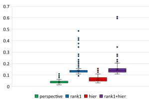
(a) Crime

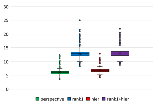
(b) Diabetes

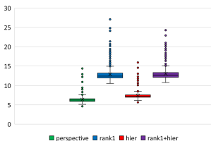
(c) Wine_quality

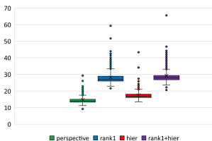
(d) Forecasting_orders

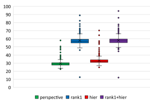
(e) Housing

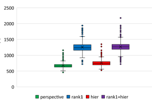
(f) Bias_correction

Figure 1: Computational times in seconds.

Figure 1 shows the distribution of times needed to solve the regression problems for each dataset. As expected, the optimal perspective formulation (24) is the fastest, as it is the simplest relaxation. We also see that formulations involving the rank-one constraints (with or without hierarchical strengthening) are more computationally demanding, taking four times longer to solve than the perspective formulation in Crime, and twice as long in the remaining five instances. In contrast, the formulation Hier, which includes hierarchical constraints but not the rank-one constraints, is much faster, requiring 70% more time than perspective in the Crime dataset, and only 10-20% more in the other instances. Indeed, there are only $\mathcal{O}(p^{2})$ hierarchical constraints to be added, while there are $\mathcal{O}(\left(p(p+3)/2\right)^{2})$ rank-one constraints.

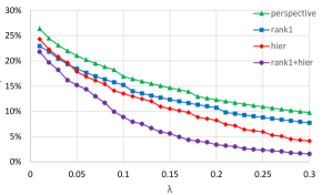
(a) Crime

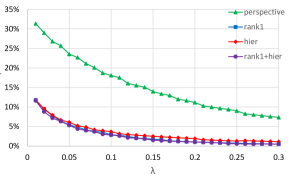
(b) Diabetes

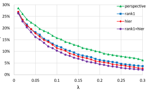
(c) Wine_quality

(d) Forecasting_orders

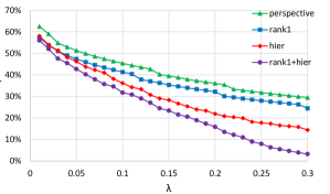
(e) Housing

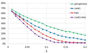
(f) Bias_correction

Figure 2: Optimality gaps as a function of $\lambda$. Each point in the graph represents the average across all values of $\mu$.

Figure 2 shows, for each dataset, the average optimality gaps as a function of the regularization parameter $\lambda$. Each point in the graph represents, for a given value of $\lambda$ the average across all 31 values of $\mu$. Similarly, Figure 3 shows, for each dataset, the average optimality gap as a function of the regularization parameter $\mu$. As expected, the optimality gaps obtained from the optimal perspective reformulation are the largest, as the relaxation (24) is dominated by all the other relaxations used. Moreover, the relaxation rank1+hier results in the smallest gaps, as it dominates every other relaxation used. Finally, neither relaxation rank1 nor hier consistently outperforms the other, although hier results in lower gaps overall in all datasets except Diabetes.

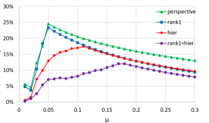
(a) Crime

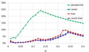
(b) Diabetes

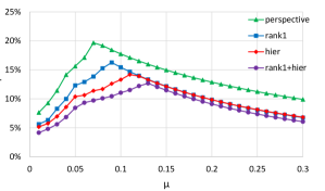
(c) Wine_quality

(d) Forecasting_orders

(e) Housing

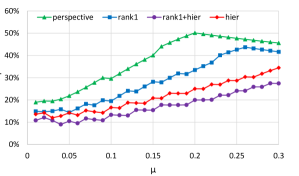
(f) Bias_correction

Figure 3: Optimality gaps as a function of $\mu$. Each point in the graph represents the average across all values of $\lambda$.

The relative performance of the formulations tested in terms of gap largely depends on the dataset and parameters used. In the Diabetes and Wine_quality datasets, the perspective reformulation is by far the worst, and all other formulations significantly improve upon it. Specifically, rank1+hier is slightly better than rank1 and hier (which have similar strengths), but the differences are marginal—observe that hier achieves an almost ideal strengthening with half the computational cost of the other formulations. In contrast, in the Crime, Housing and Bias_correction datasets, rank1 achieves only a marginal improvement over the perspective relaxation, while hier achieves a significant improvement over rank1, and rank1+hier results in a even more substantial improvement. For example, for the Housing dataset, for $\lambda=0.3$ the average optimality gap of perspective is 29%, whereas that of rank1+hier is 3%. Finally, in Forecasting_orders, all formulations perform similarly for $\lambda\leq 0.23$; however, for $\lambda\geq 0.24$, rank1+hier results in a significant improvement over the other formulations. Note that Forecasting_orders is a “fat” dataset with $n<p(p+3)/2$, which is more difficult for convexifications of the form (24) for low values of $\lambda$. Our conclusions from Figure 3 are similar. Of particular note is the marked improvement in the optimality gaps for rank1+hier over other formulations (especially perspective) for small $\mu$. For example, for $\mu=0.05$, the average optimality gap of rank1+hier in the Crime dataset is slightly over 5%, whereas hier achieves over 10% gap, and perspective and rank1 result in 25% gap.

Since hier has a similar computational cost as perspective, and rank1+hier has a virtually identical cost as rank1, we see that the hierarchical strengthening may lead to large improvements without drawbacks (whereas rank1 requires 2–4 times more computational overhead). Indeed, the hierarchical strengthening is tailored to problem (29), while rank1 is more general but does not exploit any structural information from the constraints.

Remark 1 (On rounding vs mixed-integer optimization).

An alternative to the rounding approach used here is to use mixed-integer optimization (MIO) to solve (29) exactly. An extensive comparison between MIO and the rank1 approach was performed in [5] in a variety of real datasets, including the Diabetes dataset used here. In summary, while MIO (using the perspective reformulation) was found to be more effective for large values of the parameter $\lambda$, simple rounding of the rank1 relaxation was already sufficient to prove smaller optimality gaps than MIO if $\lambda$ is small. We refer to reader to [5] for additional details.

6.2 Sparse Logistic Regression

To illustrate the convexification of non-quadratic functions derived in §2, we consider $\ell_{0}$-regularized logistic regression problems. Specifically, given a classification problem with data $(x_{i},y_{i})_{i=1}^{n}$ where $x_{i}\in\mathbb{R}^{p}$ and $y_{i}\in\{-1,1\}$, sparse logistic regression calls for solving the problem [22, 53]

$$\min_{z,\beta}\quad (1-\lambda)\sum_{i=1}^{n}\log\left(1+\exp(-y_{i}x_{i}^{\top}\beta)\right)+\lambda\sum_{i=1}^{p}z_{i}$$ (30a)

s.t. $$\beta_{i}(1-z_{i})=0,\quad\quad\forall i\in[p],$$ (30b)

where $0\leq\lambda\leq 1$ is a regularization coefficient that controls the balance between the error and the $\ell_{0}$-penalty. Note that the natural convex relaxation of (30), obtained by dropping the indicator variables $z$ (or, equivalently, adding big M constraints $|\beta_{i}|\leq Mz_{i}$ with $M\to\infty$), is convex.

To date, there are limited results concerning convexifications of (30), especially when compared with the sparse least squares regression problem (22), due to: (i) non-existence of separable terms amenable to the perspective relaxation; (ii) lack of convexifications for non-separable non-quadratic terms with indicators; and (iii) non-decomposability of the objective function into simpler terms, resulting in similar convexifications as those discussed in §5. In this paper we provided the first convexifications for non-quadratic non-separable functions, addressing issue (ii). In this section we illustrate that if the observations $x_{i}$ are sufficiently sparse, then a direct application of Theorem 1 results in substantial improvements over the natural relaxation, circumventing issues (i) and (iii).

6.2.1 Formulations

A direct application of Theorem 1, corresponding to strengthening each error term $\log\left(1+\exp(-y_{i}x_{i}^{\top}\beta)\right)\leq t_{i}$ individually, yields the following “rank-one” relaxation of the sparse logistic regression problem (30):

$$\min_{z,\beta,t}\quad (1-\lambda)\left(\sum_{i=1}^{n}t_{i}+n\log(2)\right)+\lambda\sum_{i=1}^{p}z_{i}$$ (31a)

s.t. $$t_{i}\geq\log(1+\exp(-y_{i}x_{i}^{\top}\beta))-\log(2),\quad i\in[n]$$ (31b)

$$(\textbf{log-rko})\qquad\qquad t_{i}\geq\left(\sum_{j:x_{ij}\neq 0}z_{j}\right)\log\left(1+\exp\left(-\frac{y_{i}x_{i}^{\top}\beta}{\sum_{j:x_{ij}\neq 0}z_{j}}\right)\right)$$

$$\hskip 56.9055pt-\left(\sum_{j:x_{ij}\neq 0}z_{j}\right)\log(2),\quad\hfill i\in[n]$$ (31c)

$$z_{i}\in[0,1],\quad i\in[n].$$ (31d)

We can write (31) as a conic optimization problem using the exponential cone

$$K_{exp}=\{(w_{1},w_{2},w_{3})\;|\;w_{1}\geq w_{2}e^{w_{3}/w_{2}},w_{2}>0\}\bigcup\{(w_{1},0,w_{3})\;|\;w_{1}\geq 0,w_{3}\leq 0\},$$

i.e., the closure of the set of points satisfying $w_{1}\geq w_{2}e^{w_{3}/w_{2}}$ and $w_{1},w_{2}\geq 0$.

Constraint (31b) is equivalent to $\exists u^{i}_{1},v^{i}_{1}$ such that :

$$u^{i}_{1}+v^{i}_{1}\leq 2,$$

$$(u^{i}_{1},1,-y_{i}x_{i}^{\top}\beta-t_{i})\in K_{exp},$$

$$(v^{i}_{1},1,-t_{i})\in K_{exp}.$$

Similarly, constraint (31c) is equivalent to $\exists u^{i}_{2},v^{i}_{2}$ such that:

$$u^{i}_{2}+v^{i}_{2}\leq 2(\sum_{j:x_{ij}\neq 0}z_{j}),$$

$$(u^{i}_{2},\sum_{j:x_{ij}\neq 0}z_{j},-y_{i}x_{i}^{\top}\beta-t_{i})\in K_{exp},$$

$$(v^{i}_{2},\sum_{j:x_{ij}\neq 0}z_{j},-t_{i})\in K_{exp}.$$

We refer to formulation (31) as log-rko in the sequel. We compare it with the natural convex relaxation (30) log-nat, corresponding to dropping contraints (31c) from the formulation. Observe that for relaxation log-nat, $z=\mathbf{0}$ in an optimal solution, thus resulting in the same objective value for all values of $\lambda$.

6.2.2 Lower bounds

We report lower bounds found from solving convex relaxations of (30). The optimal values of the relaxations considered are divided by $(1-\lambda)n\log(2)$. Thus the feasible solution of (30) obtained by setting $z=\beta=\mathbf{0}$ has objective value 1 (this solution may be optimal for large values of $\lambda$). The objective value of (30) also have a trivial lower bound of $0$, attained if the data can be perfectly classified (observe that if $n<p$ and $\lambda\to 0$, this lower bound may in fact be attained).

6.2.3 Instances and parameters

For the synthetic datasets, we consider the case where both the input data and the true model are sparse. Let $\alpha$ be a parameter that controls the sparsity of features $(x_{i})_{i=1}^{n}$. For each entry $x_{ij}$ we either independently assign a value of zero with probability $1-\alpha$ or we sample from a standard normal distribution $\mathcal{N}(0,1)$ with probability $\alpha$. We generate a “true” sparse coefficient vector $\beta^{*}$ with $s$ uniformly sampled non-zero indices such that $\beta^{*}_{i}=1$. The responses $y_{i}\in\{-1,1\}$ are then generated independently from a Bernoulli distribution with: $P(y_{i}=1|x_{i})=(1+\exp{(-x_{i}^{\top}\beta^{*})})^{-1}$. We use regularization values $\lambda\in\{0.1,0.3,0.5,0.7\}$ and sparsity levels $\alpha\in\{0.01,0.02,0.05,0.1\}$. Moreover, we set $p=100$, $s=1$ and test varying sample sizes $n=50,100,200$.

Table 2: Scaled lower bounds for varying $n$, $\lambda$, and $\alpha$. Each entry in the table represents the average across ten random instances.

		$\alpha=0.01$	$\alpha=0.02$	$\alpha=0.05$	$\alpha=0.1$
$n=50$
	log-nat	0.430	0.136	0.008	0
	log-rko $\lambda=0.1$	0.502	0.214	0.059	0.027
	$\lambda=0.3$	0.703	0.434	0.203	0.103
	$\lambda=0.5$	0.92	0.726	0.441	0.239
	$\lambda=0.7$	1	0.965	0.798	0.524
$n=100$
	log-nat	0.392	0.164	0.003	0
	log-rko $\lambda=0.1$	0.454	0.221	0.036	0.017
	$\lambda=0.3$	0.626	0.383	0.133	0.066
	$\lambda=0.5$	0.834	0.615	0.296	0.153
	$\lambda=0.7$	0.985	0.893	0.588	0.340
$n=200$
	log-nat	0.519	0.328	0.220	0.232
	log-rko $\lambda=0.1$	0.564	0.370	0.243	0.242
	$\lambda=0.3$	0.685	0.483	0.308	0.272
	$\lambda=0.5$	0.837	0.644	0.414	0.323
	$\lambda=0.7$	0.974	0.859	0.598	0.434

6.2.4 Results

Table 2 shows the scaled lower bounds obtained via convex relaxations log-nat and log-rko. Each entry in the table corresponds to the average (over ten replications) lower bound obtained from a given relaxation for a particular combination of sparsity level $\alpha,\lambda$, and number of observations $n$. Recall that log-nat results in the same objective regardless of the value of $\lambda$.

Compared with the natural relaxation of sparse logistic regression, the lower bound attained by (31) increases significantly when $n\leq p$. Moreover, as expected, larger improvements of log-rko over log-nat are obtained for larger values of $\lambda$, where sparsity plays a more prominent role in the objective value. The lower bounds of log-rko are at least $16\%$ more than those of log-nat in all test cases, and sometimes substantially larger (e.g., in cases log-nat results in the trivial lower bound of $0$). When the input data is very sparse, i.e., $\alpha=0.01$ and $\lambda\geq 0.5$, log-rko results in lower bounds close to $1$ or equal to $1$, suggesting (and in some cases proving) that true optimal solution in those cases is $z=\beta=\mathbf{0}$. When $n>p$, log-rko still results in better lower bounds than log-nat, although improvements are less pronounced in these cases.

7 Conclusions

In this paper, we propose a unifying convexification technique for the epigraphs of a class of convex functions with indicator variables constrained to certain polyhedral sets. We illustrate the utility of our approaches on constrained regression problems of recent interest. Our results generalize the existing results that consider only quadratic, separable or differentiable convex functions, and certain structural constraints such as cardinality or unit commitment. As future research, we plan to consider convexifications for more general functions.

Appendix A The special case when $\text{conv}(Q)$ is compact

In this section, we give an extended formulation of $\operatorname{cl\ conv}(Z_{Q})$ based on an extended formulation of $\text{conv}(Q_{0})$. In particular, this alternative formulation is more favorable in cases when the number of facets of $\text{conv}(Q)$ is polynomially bounded while $\text{conv}(Q_{0})$ has an exponential number of facets. We denote the facets of $\text{conv}(Q)$ which do not contain zero by $\{F_{\ell}\}_{1\leq\ell\leq k}$, and we write each $F_{\ell}$ as $F_{\ell}:=\{z\;|\;A_{\ell}z\leq b_{\ell}\}$. Angulo et al., [2] prove that $\text{conv}(Q_{0})=\text{conv}\left(\bigcup_{1\leq\ell\leq k}F_{\ell}\right)$, and a natural extended formulation of $\text{conv}(Q_{0})$ is as follows:

$$z=\sum_{\ell\in[k]}\hat{z}_{\ell}$$ (32a)

$$A_{\ell}\hat{z}_{\ell}\leq\lambda_{\ell}b_{\ell} \ell\in[k]$$ (32b)

$$\sum_{\ell\in[k]}\lambda_{\ell}=1,\;\lambda\geq\mathbf{0}.$$ (32c)

Theorem 4.

$$\operatorname{cl\ conv}(Z_{Q})=\operatorname{proj}_{(z,\beta,t)}\Big{\{}(z,\hat{z},\lambda,\beta,t)\in\mathbb{R}_{+}^{(k+1)p+k} \times\mathbb{R}^{p}\times\mathbb{R}\;|\;\eqref{eq:ExtendedQ0-1}\--\eqref{eq:ExtendedQ0-2},\;\sum_{\ell\in[k]}\lambda_{\ell}\leq 1,$$

$$t\geq f(\mathbf{1}^{\top}\beta),\;t\geq(\mathbf{1}^{\top}\lambda)f\left(\frac{\mathbf{1}^{\top}\beta}{\mathbf{1}^{\top}\lambda}\right)\Big{\}}.$$

Proof.

Let

$$Z=\Big{\{}(z,\hat{z},\lambda,\beta,t)\in\mathbb{R}_{+}^{(k+1)p+k}\times\mathbb{R}^{p}\times\mathbb{R}\;|\; \eqref{eq:ExtendedQ0-1}\--\eqref{eq:ExtendedQ0-2},\;\sum_{\ell\in[k]}\lambda_{\ell}\leq 1,t\geq f(\mathbf{1}^{\top}\beta),$$

$$t\geq(\mathbf{1}^{\top}\lambda)f\left(\frac{\mathbf{1}^{\top}\beta}{\mathbf{1}^{\top}\lambda}\right)\Big{\}}.$$

First we show that $\operatorname{proj}_{(z,\beta,t)}(Z)\subseteq\operatorname{cl\ conv}(Z_{Q})$. Given any $(z,\hat{z},\lambda,\beta,t)\in Z$, note that constraints $z\in\text{conv}(Q)$ and $t\geq f(\mathbf{1}^{\top}\beta)$ defining $\operatorname{cl\ conv}(Z_{Q})$ are trivially satisfied. It remains to show that $t\geq(\pi^{\top}z)f\left(\frac{\mathbf{1}^{\top}\beta}{\pi^{\top}z}\right),\;\;\forall\pi\in\mathcal{F}$. For each $\pi\in\mathcal{F}$, we have

$$\pi^{\top}z=\sum_{\ell\in[k]}\pi^{\top}\hat{z}_{\ell}=\sum_{\ell\in[k]}\lambda_{\ell}\pi^{\top}\left(\frac{\hat{z}_{\ell}}{\lambda_{\ell}}\right)\geq\sum_{\ell\in[k]}\lambda_{\ell},$$

where the inequality follows from the fact that we must have either $\lambda_{\ell}=0$ and $\hat{z}_{\ell}=\mathbf{0}$ or $\lambda_{\ell}>0$ and $\frac{\hat{z}_{\ell}}{\lambda_{\ell}}\in F_{\ell}$ since each $F_{\ell}$ is a polytope contained in the half-space defined by inequality $\mathbf{1}^{\top}z\geq 1$. Thus, from Lemma 1, we have $t\geq(\mathbf{1}^{\top}\lambda)f\left(\frac{\mathbf{1}^{\top}\beta}{\mathbf{1}^{\top}\lambda}\right)\geq(\pi^{\top}z)f\left(\frac{\mathbf{1}^{\top}\beta}{\pi^{\top}z}\right),\;\;\forall\pi\in\mathcal{F}$, hence $\operatorname{proj}_{(z,\beta,t)}(Z)\subseteq\operatorname{cl\ conv}(Z_{Q})$.

Now, it remains to prove that $\operatorname{cl\ conv}(Z_{Q})\subseteq\operatorname{proj}_{(z,\beta,t)}(Z)$. For any $(z,\beta,t)\in\operatorname{cl\ conv}(Z_{Q})$ if $z\in\text{conv}(Q_{0})$, then there exist $\hat{z}_{\ell}$ and $\lambda_{\ell}$ that satisfy (32) and $\mathbf{1}^{\top}\lambda=1$. Since $t\geq f(\mathbf{1}^{\top}\beta)$ for all $(z,\beta,t)\in\operatorname{cl\ conv}(Z_{Q})$, $(z,\beta,t)\in\operatorname{proj}_{(z,\beta,t)}(Z)$. If $z\in\text{conv}(Q)\backslash\text{conv}(Q_{0})$, then, from Lemma 2, we can write $z$ as $z=\lambda_{0}z_{0}$, $0\leq\lambda_{0}<1$, and we may assume $z_{0}$ is on one of the facets of $\text{conv}(Q_{0})$ defined by $\hat{\pi}^{\top}z_{0}=1$ for some $\hat{\pi}\in\mathcal{F}$. By definition, $\forall\pi\in\mathcal{F}\;\;$ $\pi^{\top}z_{0}\geq\hat{\pi}^{\top}z_{0}=1$ which implies $\lambda_{0}=\hat{\pi}^{\top}z=\min_{\pi\in\mathcal{F}}\pi^{\top}z$. Since $z_{0}\in\text{conv}(Q_{0})$, there exists $\hat{z}_{\ell},\lambda_{\ell}$ such that $z_{0}=\sum_{\ell\in[k]}\hat{z}_{\ell}$ and (32b)–(32c) hold. Then

$$z= \sum_{\ell\in[k]}(\lambda_{0}\hat{z}_{\ell})$$

$$A_{\ell}(\lambda_{0}\hat{z}_{\ell})\leq\lambda_{0}\lambda_{\ell}b_{\ell}, \ell\in[k]$$

$$\sum_{\ell\in[k]}\lambda_{0}\lambda_{\ell}\leq 1,\lambda\geq\mathbf{0},$$

and we have $\sum_{\ell\in[k]}\lambda_{0}\lambda_{\ell}=\lambda_{0}=\min_{\pi\in\mathcal{F}}\pi^{\top}z$. Using Lemma 1, we find that $t\geq(\pi^{\top}z)f\left(\frac{\mathbf{1}^{\top}\beta}{\pi^{\top}z}\right),\;\;\forall\pi\in\mathcal{F}$ implies that $t\geq(\sum_{\ell\in[k]}\lambda_{0}\lambda_{\ell})f\left(\frac{\mathbf{1}^{\top}\beta}{\sum_{\ell\in[k]}\lambda_{0}\lambda_{\ell}}\right)\geq(\sum_{\ell\in[k]}\lambda_{\ell})f\left(\frac{\mathbf{1}^{\top}\beta}{\sum_{\ell\in[k]}\lambda_{\ell}}\right)$. Hence, $(z,\beta,t)\in\operatorname{proj}_{(z,\beta,t)}(Z)$.

∎

References

• Aktürk et al., [2009] Aktürk, M. S., Atamtürk, A., and Gürel, S. (2009). A strong conic quadratic reformulation for machine-job assignment with controllable processing times. Operations Research Letters, 37(3):187–191.
• Angulo et al., [2015] Angulo, G., Ahmed, S., Dey, S. S., and Kaibel, V. (2015). Forbidden vertices. Mathematics of Operations Research, 40(2):350–360.
• Anstreicher, [2012] Anstreicher, K. M. (2012). On convex relaxations for quadratically constrained quadratic programming. Mathematical Programming, 136(2):233–251.
• Atamtürk and Gómez, [2018] Atamtürk, A. and Gómez, A. (2018). Strong formulations for quadratic optimization with M-matrices and indicator variables. Mathematical Programming, 170(1):141–176.
• Atamtürk and Gómez, [2019] Atamtürk, A. and Gómez, A. (2019). Rank-one convexification for sparse regression. Optimization Online. http://www.optimization-online.org/DB_HTML/2019/01/7050.html.
• Atamtürk et al., [2021] Atamtürk, A., Gómez, A., and Han, S. (2021). Sparse and smooth signal estimation: Convexification of L0 formulations. Journal of Machine Learning Research, 3:1–43.
• Bacci et al., [2019] Bacci, T., Frangioni, A., Gentile, C., and Tavlaridis-Gyparakis, K. (2019). New MINLP formulations for the unit commitment problems with ramping constraints. Optimization Online. http://www.optimization-online.org/DB_FILE/2019/10/7426.pdf.
• Belotti et al., [2015] Belotti, P., Góez, J. C., Pólik, I., Ralphs, T. K., and Terlaky, T. (2015). A conic representation of the convex hull of disjunctive sets and conic cuts for integer second order cone optimization. In Numerical Analysis and Optimization, pages 1–35. Springer.
• [9] Bertsimas, D., Cory-Wright, R., and Pauphilet, J. (2020a). Mixed-projection conic optimization: A new paradigm for modeling rank constraints. arXiv preprint arXiv:2009.10395.
• Bertsimas and King, [2016] Bertsimas, D. and King, A. (2016). OR Forum – An algorithmic approach to linear regression. Operations Research, 64(1):2–16.
• Bertsimas et al., [2016] Bertsimas, D., King, A., and Mazumder, R. (2016). Best subset selection via a modern optimization lens. The Annals of Statistics, 44(2):813–852.
• [12] Bertsimas, D., Pauphilet, J., Van Parys, B., et al. (2020b). Sparse regression: Scalable algorithms and empirical performance. Statistical Science, 35(4):555–578.
• Bertsimas and Van Parys, [2017] Bertsimas, D. and Van Parys, B. (2017). Sparse high-dimensional regression: Exact scalable algorithms and phase transitions. arXiv preprint arXiv:1709.10029.
• Bien et al., [2013] Bien, J., Taylor, J., and Tibshirani, R. (2013). A lasso for hierarchical interactions. Annals of Statistics, 41(3):1111.
• Bienstock and Michalka, [2014] Bienstock, D. and Michalka, A. (2014). Cutting-planes for optimization of convex functions over nonconvex sets. SIAM Journal on Optimization, 24(2):643–677.
• Burer, [2009] Burer, S. (2009). On the copositive representation of binary and continuous nonconvex quadratic programs. Mathematical Programming, 120(2):479–495.
• Burer and Kılınç-Karzan, [2017] Burer, S. and Kılınç-Karzan, F. (2017). How to convexify the intersection of a second order cone and a nonconvex quadratic. Mathematical Programming, 162(1-2):393–429.
• Carrizosa et al., [2020] Carrizosa, E., Mortensen, L., and Morales, D. R. (2020). On linear regression models with hierarchical categorical variables. Technical report.
• Ceria and Soares, [1999] Ceria, S. and Soares, J. (1999). Convex programming for disjunctive convex optimization. Mathematical Programming, 86:595–614.
• Cozad et al., [2014] Cozad, A., Sahinidis, N. V., and Miller, D. C. (2014). Learning surrogate models for simulation-based optimization. AIChE Journal, 60(6):2211–2227.
• Cozad et al., [2015] Cozad, A., Sahinidis, N. V., and Miller, D. C. (2015). A combined first-principles and data-driven approach to model building. Computers & Chemical Engineering, 73:116–127.
• Dedieu et al., [2020] Dedieu, A., Hazimeh, H., and Mazumder, R. (2020). Learning sparse classifiers: Continuous and mixed integer optimization perspectives. arXiv preprint arXiv:2001.06471.
• Dheeru and Karra Taniskidou, [2017] Dheeru, D. and Karra Taniskidou, E. (2017). UCI machine learning repository.
• Dong, [2019] Dong, H. (2019). On integer and MPCC representability of affine sparsity. Operations Research Letters, 47(3):208–212.
• Dong et al., [2019] Dong, H., Ahn, M., and Pang, J.-S. (2019). Structural properties of affine sparsity constraints. Mathematical Programming, 176(1-2):95–135.
• Dong et al., [2015] Dong, H., Chen, K., and Linderoth, J. (2015). Regularization vs. relaxation: A conic optimization perspective of statistical variable selection. arXiv preprint arXiv:1510.06083.
• Dong and Linderoth, [2013] Dong, H. and Linderoth, J. (2013). On valid inequalities for quadratic programming with continuous variables and binary indicators. In Goemans, M. and Correa, J., editors, Integer Programming and Combinatorial Optimization, pages 169–180, Berlin, Heidelberg. Springer.
• Efron et al., [2004] Efron, B., Hastie, T., Johnstone, I., and Tibshirani, R. (2004). Least angle regression. The Annals of Statistics, 32(2):407–499.
• Fan and Li, [2001] Fan, J. and Li, R. (2001). Variable selection via nonconcave penalized likelihood and its oracle properties. Journal of the American Statistical Association, 96(456):1348–1360.
• Frangioni et al., [2016] Frangioni, A., Furini, F., and Gentile, C. (2016). Approximated perspective relaxations: a project and lift approach. Computational Optimization and Applications, 63(3):705–735.
• Frangioni and Gentile, [2006] Frangioni, A. and Gentile, C. (2006). Perspective cuts for a class of convex 0–1 mixed integer programs. Mathematical Programming, 106:225–236.
• Frangioni and Gentile, [2007] Frangioni, A. and Gentile, C. (2007). SDP diagonalizations and perspective cuts for a class of nonseparable MIQP. Operations Research Letters, 35(2):181–185.
• Frangioni and Gentile, [2009] Frangioni, A. and Gentile, C. (2009). A computational comparison of reformulations of the perspective relaxation: SOCP vs. cutting planes. Operations Research Letters, 37(3):206–210.
• Frangioni et al., [2011] Frangioni, A., Gentile, C., Grande, E., and Pacifici, A. (2011). Projected perspective reformulations with applications in design problems. Operations Research, 59(5):1225–1232.
• Frangioni et al., [2020] Frangioni, A., Gentile, C., and Hungerford, J. (2020). Decompositions of semidefinite matrices and the perspective reformulation of nonseparable quadratic programs. Mathematics of Operations Research, 45(1):15–33.
• Günlük and Linderoth, [2010] Günlük, O. and Linderoth, J. (2010). Perspective reformulations of mixed integer nonlinear programs with indicator variables. Mathematical Programming, 124:183–205.
• Han et al., [2020] Han, S., Gómez, A., and Atamtürk, A. (2020). 2x2 convexifications for convex quadratic optimization with indicator variables. arXiv preprint arXiv:2004.07448.
• Hardy, [1908] Hardy, G. H. (1908). Course of Pure Mathematics. Courier Dover Publications.
• Hastie et al., [2015] Hastie, T., Tibshirani, R., and Wainwright, M. (2015). Statistical Learning with Sparsity: The Lasso and Generalizations. Monographs on statistics and applied probability, no. 143. Chapman and Hall/CRC.
• Hazimeh and Mazumder, [2020] Hazimeh, H. and Mazumder, R. (2020). Learning hierarchical interactions at scale: A convex optimization approach. In Chiappa, S. and Calandra, R., editors, Proceedings of the Twenty Third International Conference on Artificial Intelligence and Statistics, volume 108 of Proceedings of Machine Learning Research, pages 1833–1843. PMLR.
• Hazimeh et al., [2020] Hazimeh, H., Mazumder, R., and Saab, A. (2020). Sparse regression at scale: Branch-and-bound rooted in first-order optimization. arXiv preprint arXiv:2004.06152.
• Hijazi et al., [2012] Hijazi, H., Bonami, P., Cornuéjols, G., and Ouorou, A. (2012). Mixed-integer nonlinear programs featuring “on/off” constraints. Computational Optimization and Applications, 52(2):537–558.
• Huang et al., [2012] Huang, J., Breheny, P., and Ma, S. (2012). A selective review of group selection in high-dimensional models. Statistical science: A Review Journal of the Institute of Mathematical Statistics, 27(4).
• Jeon et al., [2017] Jeon, H., Linderoth, J., and Miller, A. (2017). Quadratic cone cutting surfaces for quadratic programs with on–off constraints. Discrete Optimization, 24:32–50.
• Kılınç-Karzan and Yıldız, [2014] Kılınç-Karzan, F. and Yıldız, S. (2014). Two-term disjunctions on the second-order cone. In International Conference on Integer Programming and Combinatorial Optimization, pages 345–356. Springer.
• Küçükyavuz et al., [2020] Küçükyavuz, S., Shojaie, A., Manzour, H., and Wei, L. (2020). Consistent second-order conic integer programming for learning Bayesian networks. arXiv preprint arXiv:2005.14346.
• Manzour et al., [2021] Manzour, H., Küçükyavuz, S., Wu, H.-H., and Shojaie, A. (2021). Integer programming for learning directed acyclic graphs from continuous data. INFORMS Journal on Optimization, 3(1):46–73.
• Miller, [2002] Miller, A. (2002). Subset selection in regression. Chapman and Hall/CRC.
• Modaresi et al., [2016] Modaresi, S., Kılınç, M. R., and Vielma, J. P. (2016). Intersection cuts for nonlinear integer programming: Convexification techniques for structured sets. Mathematical Programming, 155(1-2):575–611.
• Natarajan, [1995] Natarajan, B. K. (1995). Sparse approximate solutions to linear systems. SIAM Journal on Computing, 24(2):227–234.
• Pilanci et al., [2015] Pilanci, P., Wainwright, M. J., and El Ghaoui, L. (2015). Sparse learning via boolean relaxations. Mathematical Programming, 151:63–87.
• Richard and Tawarmalani, [2010] Richard, J.-P. P. and Tawarmalani, M. (2010). Lifting inequalities: a framework for generating strong cuts for nonlinear programs. Mathematical Programming, 121(1):61–104.
• Sato et al., [2016] Sato, T., Takano, Y., Miyashiro, R., and Yoshise, A. (2016). Feature subset selection for logistic regression via mixed integer optimization. Computational Optimization and Applications, 64(3):865–880.
• Stubbs and Mehrotra, [1999] Stubbs, R. A. and Mehrotra, S. (1999). A branch-and-cut method for 0-1 mixed convex programming. Mathematical Programming, 86(3):515–532.
• Tibshirani, [1996] Tibshirani, R. (1996). Regression shrinkage and selection via the lasso. Journal of the Royal Statistical Society: Series B (Methodological), pages 267–288.
• Vielma, [2019] Vielma, J. P. (2019). Small and strong formulations for unions of convex sets from the Cayley embedding. Mathematical Programming, 177(1-2):21–53.
• [57] Wang, A. L. and Kılınç-Karzan, F. (2020a). The generalized trust region subproblem: solution complexity and convex hull results. Forthcoming in Mathematical Programming.
• [58] Wang, A. L. and Kılınç-Karzan, F. (2020b). On convex hulls of epigraphs of QCQPs. In Bienstock, D. and Zambelli, G., editors, Integer Programming and Combinatorial Optimization, pages 419–432, Cham. Springer International Publishing.
• Wang and Kılınç-Karzan, [2021] Wang, A. L. and Kılınç-Karzan, F. (2021). On the tightness of SDP relaxations of QCQPs. Forthcoming in Mathematical Programming.
• Wei et al., [2020] Wei, L., Gómez, A., and Küçükyavuz, S. (2020). On the convexification of constrained quadratic optimization problems with indicator variables. In Bienstock, D. and Zambelli, G., editors, Integer Programming and Combinatorial Optimization, pages 433–447, Cham. Springer International Publishing.
• Wu et al., [2017] Wu, B., Sun, X., Li, D., and Zheng, X. (2017). Quadratic convex reformulations for semicontinuous quadratic programming. SIAM Journal on Optimization, 27(3):1531–1553.
• Xie and Deng, [2020] Xie, W. and Deng, X. (2020). Scalable algorithms for the sparse ridge regression. SIAM Journal on Optimization, 30(4):3359–3386.
• Zhang, [2010] Zhang, C.-H. (2010). Nearly unbiased variable selection under minimax concave penalty. The Annals of Statistics, 38:894–942.
• Zheng et al., [2014] Zheng, X., Sun, X., and Li, D. (2014). Improving the performance of MIQP solvers for quadratic programs with cardinality and minimum threshold constraints: A semidefinite program approach. INFORMS Journal on Computing, 26(4):690–703.