Sparse Approximate Multifrontal Factorization with Butterfly Compression for High Frequency Wave Equations

Abstract

We present a fast and approximate multifrontal solver for large-scale sparse linear systems arising from finite-difference, finite-volume or finite-element discretization of high-frequency wave equations. The proposed solver leverages the butterfly algorithm and its hierarchical matrix extension for compressing and factorizing large frontal matrices via graph-distance guided entry evaluation or randomized matrix-vector multiplication-based schemes. Complexity analysis and numerical experiments demonstrate $\mathcal{O}(N\log^{2}N)$ computation and $\mathcal{O}(N)$ memory complexity when applied to an $N\times N$ sparse system arising from 3D high-frequency Helmholtz and Maxwell problems.

15A23, 65F50, 65R10, 65R20

1 Introduction

Direct solution of large sparse linear systems arsing from e.g., finite-difference, finite-element or finite-volume discretization of partial differential equations (PDE) is crucial for many high-performance scientific and engineering simulation codes. Efficient solution of these sparse systems often requires reordering the matrix to improve numerical stability and fill-in ratios, and performing the computations on smaller but dense submatrices to improve flop performance. Examples include supernodal and multifrontal methods that perform operations on so-called supernodes and frontal matrices, respectively [17, 14]. For multifrontal methods [36], the size $n$ of the frontal matrices can grow as $n=\mathcal{O}(N^{1/2})$ and $n=\mathcal{O}(N^{2/3})$ for typical 2D and 3D PDEs with $N$ denoting the system size. Performing dense factorization and solution on the frontal matrices requires $\mathcal{O}(n^{3})$ operations, yielding the overall complexities of $\mathcal{O}(N^{3/2})$ in 2D and $\mathcal{O}(N^{2})$ in 3D. The same complexities also apply to supernodal methods.

For many applications arising from wide classes of PDEs, these complexities can be reduced by leveraging algebraic compression tools to exploit rank structures in blocks of the matrix inverse. For example, it can be rigorously shown that, for elliptical PDEs with constant or smooth coefficients, certain off-diagonal blocks in a frontal matrix exhibit low-rankness [13]. Low-rank based fast direct solvers, including $\mathcal{H}$ [25, 20] and $\mathcal{H}^{2}$ matrices [26], hierarchically off-diagonal low-rank (HOD-LR) formats [1], sequentially semi-separable formats [52], hierarchically semi-separable (HSS) formats [52], and block low-rank (BLR) formats [48, 2, 3], represent off-diagonal blocks as low-rank products and leverage fast algebras to perform efficient matrix factorization. These methods were first developed to address dense systems, e.g., arising from boundary element methods, in quasi-linear complexity and have been recently adapted for sparse systems. Examples include solvers coupling $\mathcal{H}$ [58], HOD-LR [5], HSS [54, 53, 19] or BLR [2] with multifrontal methods, which we will refer to as rank structured multifrontal methods, and solvers coupling HOD-LR [12] or BLR [43] with supernodal methods, solvers based on the inverse fast multipole method [47], and multifrontal-like solvers based on hierarchical interpolative factorization (HIF) [31, 35]. Available software packages include STRUMPACK [19], MUMPS [2], and PaStiX [29, 43]. It is worth mentioning that many of these methods rely on fast entry evaluation or randomized matrix vector multiplication (matvec) to compress the frontal matrices, without explicitly forming them. Despite differences in the leading constants, implementation details and applicability of these compression formats, in general they lead to quasi-linear complexity direct solvers and preconditioners when applied to many elliptical PDEs. Unfortunately, when applied to wave equations, such as Helmholtz, Maxwell, or Schrödinger equations with constant or non-constant coefficients, the frontal matrices exhibit much higher numerical ranks due to the highly oscillatory nature of the numerical Green’s function [18] and consequently no asymptotic complexity reduction compared to the exact sparse solvers can be attained. That said, the low-rank based sparse direct solver packages (e.g., STRUMPACK and MUMPS) oftentimes significantly reduce the costs of exact sparse solvers for practical wave equation systems [45], and scale quasi-linearly when the 3D computation domain spans less than a few wavelengths.

In contrast to low-rank-based algorithms, we consider another algebraic compression tool called butterfly [41, 38, 34, 33, 46], for constructing fast multifrontal methods for wave equations. Butterfly is a multilevel matrix decomposition algorithm well-suited for representing highly oscillatory operators such as Fourier transforms and integral operators [11, 56, 55] and special function transforms [51, 8, 44]. When combined with hierarchical matrix techniques, butterfly can also serve as the building block for accelerating iterative methods [42], direct solvers [21, 22, 24, 37] and preconditioners [39] for boundary element methods for high-frequency wave equations. These techniques essentially replace low-rank products in the $\mathcal{H}$ [22], $\mathcal{H}^{2}$ [57, 10] and HOD-LR formats [37] with butterflies, and leverage fast and randomized butterfly algebra to compute the matrix inverse (for direct solvers and preconditioners). We particularly focus on the butterfly extension of the HOD-LR format [37], called HOD-BF in this paper. The HOD-BF format yields smaller leading constants and better parallel performance compared to other butterfly-enhanced hierarchical matrix formats. Moreover, HOD-BF can attain an $\mathcal{O}(n\log^{2}n)$ compression complexity and an empirical $\mathcal{O}(n^{3/2}\log n)$ inversion complexity given an $n\times n$ HOD-BF compressible dense matrix. HOD-BF has been previously applied to both 2D [37] and 3D boundary element methods.

In this paper, we leverage the HOD-BF format for compressing the frontal matrices in the multifrontal method. The proposed algorithm is formulated as Algorithm 5, which combines several butterfly algorithms at multiple phases of the multifrontal method. Specifically, any non-root frontal matrix has a $2\times 2$ blocked partition, and each block represents numerical Green’s function interactions between unknowns residing on planar or crossing planes (or lines). These blocks are compressed as butterfly or HOD-BF by extracting selected matrix entries [41, 46], from the children frontal matrices and the original sparse matrix. Moreover, the method factorizes the leading diagonal block using the HOD-BF inversion technique [37] and compute its Schur complement with the randomized butterfly construction algorithm [38]. It’s worth mentioning that efficient integration of butterfly algorithms into the multifrontal method requires several algorithmic innovations. First, butterfly construction of frontal blocks requires sub-sampling matrix entries using proxy rows and columns to maintain quasi-linear complexities. These proxies are selected by combining uniform sampling and nearest neighbor sampling, computed using the graph distance (see Algorithm 2). Second, matrix sub-sampling boils down to extracting entries from the compressed children frontal matrices, implemented as partial matvec in a blocked and parallel fashion (Algorithm 3).

Given a frontal matrix of size $n\times n$, the construction and factorization can be performed in $\mathcal{O}(n^{3/2}\log n)$ complexity. Consequently, for a sparse matrix resulting from 2D and 3D high frequency wave equations, the solver can attain an overall complexity of $\mathcal{O}(N)$ and $\mathcal{O}(N\log^{2}N)$, respectively. It is worth mentioning the same complexities can be attained for 2D and 3D low-frequency or static PDEs such as the Poisson equation. To the best of our knowledge, the proposed solver represents the first-ever quasi-linear complexity multifrontal solver for high-frequency wave equations in 3D.

As a related work, the sweeping preconditioner-based domain decomposition solvers [50] represent another quasi-linear complexity technique for wave equations and impressive numerical results have been reported for both 2D and 3D cases. However, sweeping preconditioners only apply to regular grids and domains and do not work well for domains containing resonant cavities. In comparison, the proposed solver does not suffer from these constraints and applies to wider classes of applications. In addition, the proposed solver can be used inside domain decomposition solvers, which often use multifrontal solvers for their local sparse systems.

The rest of the paper is organized as follows. The multifrontal method is presented in Section 2. The butterfly format, construction and entry extraction algorithms are described in Section 3, followed by their generalization to the HOD-BF format in Section 4. The proposed rank structured multifrontal method is detailed in Section 5, including complexity analysis. Numerical results demonstrating the efficiency and applicability of the proposed solver for the 3D Helmholtz, Maxwell, and Poisson equations are presented in Section 6, followed by conclusions in Section 7.

2 Sparse Multifrontal LU Factorization

We consider the LU factorization of a sparse matrix $A\in\mathbb{C}^{N\times N}$, as $P\left(D_{r}AD_{c}Q_{c}\right)P^{\top}=LU$, where $P$ and $Q_{c}$ are permutation matrices, $D_{r}$ and $D_{c}$ are diagonal row and column scaling matrices and $L$ and $U$ are sparse lower and upper-triangular respectively. $Q_{c}$ aims to maximize the magnitude of the elements on the matrix diagonal. $D_{r}$ and $D_{c}$ scale the matrix such that the diagonal entries are one in absolute value and all off-diagonal entries are less than one. This step is implemented using the sequential MC64 code [15] or the parallel method – without the diagonal scaling – described in [7]. The permutation $P$ is applied symmetrically and is used to minimize the fill-in, i.e., the number of non-zero entries in the sparse factors $L$ and $U$. This permutation is computed from the symmetric sparsity structure of $A+A^{\top}$. For large problems the preferred ordering is typically based on the nested dissection heuristic, as implemented in METIS [32] or Scotch.

The multifrontal method [16] relies on a graph called the assembly tree to guide the computation. Each node $\tau$ of the assembly tree corresponds to a dense frontal matrix $F_{\tau}$, representing an intermediate dense submatrix in sparse Gaussian elimination, with the following $2\times 2$ block structure: $F_{\tau}=\begin{bmatrix}F_{11}&F_{12}\\ F_{21}&F_{22}\end{bmatrix}$. Here, the rows and columns corresponding to the $F_{11}$ block, denoted by index set $I^{s}_{\tau}$, are called the fully-summed variables, and when the front is constructed, $F_{11}$ is ready for LU factorization. The disjoint index sets $I^{s}_{\tau}$ form a partition of the index set of $A$ as $\bigcup_{\tau}I^{s}_{\tau}=\{1,\dots,N\}$. In the context of nested dissection, the sets $I_{\tau}^{s}$ correspond to individual vertex separators. The rows and columns corresponding to the $F_{22}$ block, denoted by index set $I^{u}_{\tau}$, define the (temporary) Schur complement update blocks that $F_{11}$ contributes to during the multifrontal LU factorization. Let $C_{\tau}=F_{22}-F_{21}F_{11}^{-1}F_{12}$ denote the contribution block, i.e., the Schur complement updated $F_{22}$. If $\nu$ is a child of $\tau$ in the assembly tree, then $I^{u}_{\nu}\subset\{I^{s}_{\tau}\cup I^{u}_{\tau}\}$; for the root node $t$, $I_{t}^{u}\equiv\emptyset$. Let $\#I^{\text{s}}_{\tau}$, $\#I^{\text{u}}_{\tau}$ and $n_{\tau}=\#I^{\text{s}}_{\tau}\,+\,\#I^{\text{u}}_{\tau}$ denote the dimensions of $F_{11}$, $F_{22}$ and $F_{\tau}$, respectively. Note that $n_{\tau}$ tends to get bigger toward the root of the assembly tree. When considering a single front, we will omit the $\tau$ subscript.

The multifrontal method casts the factorization of a sparse matrix into a series of partial factorizations and Schur complement updates of the frontal matrices. It consists in a bottom-up traversal of the assembly tree following a topological order. Processing a node consists of four steps:

1. Assembling the frontal matrix $F_{\tau}$, i.e., combining elements from the sparse matrix $A$ with the children’s ($\nu_{1}$ and $\nu_{2}$) contribution blocks. This involves a scatter operation and is called extend-add, denoted by $\mathbin{\hskip 6.49994pt\text{\makebox[0.0pt]{\leavevmode\resizebox{3.00003pt}{8.50006pt}{$\updownarrow$}}\raisebox{1.49994pt}{\makebox[0.0pt]{\leavevmode\resizebox{13.00005pt}{1.99997pt}{$\leftrightarrow$}}}}\hskip 6.49994pt}$:

   $$F_{\tau}=\begin{bmatrix}A(I^{s}_{\tau},I^{s}_{\tau})&A(I^{s}_{\tau},I^{u}_{\tau})\\ A(I^{u}_{\tau},I^{s}_{\tau})\end{bmatrix}\mathbin{\hskip 6.49994pt\text{\makebox[0.0pt]{\leavevmode\resizebox{3.00003pt}{8.50006pt}{$\updownarrow$}}\raisebox{1.49994pt}{\makebox[0.0pt]{\leavevmode\resizebox{13.00005pt}{1.99997pt}{$\leftrightarrow$}}}}\hskip 6.49994pt}F_{22;\nu_{1}}\mathbin{\hskip 6.49994pt\text{\makebox[0.0pt]{\leavevmode\resizebox{3.00003pt}{8.50006pt}{$\updownarrow$}}\raisebox{1.49994pt}{\makebox[0.0pt]{\leavevmode\resizebox{13.00005pt}{1.99997pt}{$\leftrightarrow$}}}}\hskip 6.49994pt}F_{22;\nu_{2}}=\leavevmode\hbox to34.54pt{\vbox to34.54pt{\text{[drawing]}}}\mathbin{\hskip 6.49994pt\text{\makebox[0.0pt]{\leavevmode\resizebox{3.00003pt}{8.50006pt}{$\updownarrow$}}\raisebox{1.49994pt}{\makebox[0.0pt]{\leavevmode\resizebox{13.00005pt}{1.99997pt}{$\leftrightarrow$}}}}\hskip 6.49994pt}\leavevmode\hbox to23.16pt{\vbox to23.16pt{\text{[drawing]}}}\mathbin{\hskip 6.49994pt\text{\makebox[0.0pt]{\leavevmode\resizebox{3.00003pt}{8.50006pt}{$\updownarrow$}}\raisebox{1.49994pt}{\makebox[0.0pt]{\leavevmode\resizebox{13.00005pt}{1.99997pt}{$\leftrightarrow$}}}}\hskip 6.49994pt}\leavevmode\hbox to27.43pt{\vbox to27.43pt{\text{[drawing]}}}$$

2. Elimination of the fully-summed variables in the $F_{11}$ block, i.e., dense LU factorization with partial pivoting of $F_{11}$.

3. Updating the off-diagonal blocks $F_{12}$ and $F_{21}$.

4. Computing the contribution block from the Schur complement update of $F_{22}$: $C_{\tau}=F_{22}-F_{21}F_{11}^{-1}F_{12}$. $C_{\tau}$ or $F_{22}$ is temporary storage (pushed on a stack), and can be released as soon as it has been used in the front assembly (step (1)) of the parent node.

After the numerical factorization, the lower triangular sparse factor is available in the $F_{21}$ and $F_{11}$ blocks and the upper triangular factor in the $F_{11}$ and $F_{12}$ blocks. These can then be used to very efficiently solve linear systems, using forward and backward substitution. A high-level overview is given in Algorithm 1.

We implemented the multifrontal method in the STRUMPACK library [49], using C++, MPI and OpenMP, supporting real/complex arithmetic, single/double precision and $32$/$64$-bit integers. Note that the pivoting strategy in factorization of $F_{11}$ in STRUMPACK does not use numerical values of $F_{21}$ and $F_{12}$ for ease of implementation.

For any frontal matrix $F_{\tau}$ of size $n_{\tau}$, its LU factorization (only on $F_{11}$) and storage costs scale as $\mathcal{O}(n_{\tau}^{3})$ and $\mathcal{O}(n_{\tau}^{2})$, severely limiting the applicability of the multifrontal method to large-scale PDE problems. In what follows, we leverage the butterfly algorithm and its hierarchical matrix extension for representing frontal matrices and constructing fast sparse direct solvers, particularly for high-frequency wave equations.

Input: $A\in\mathbb{R}^{N\times N}$, $b\in\mathbb{R}^{N}$
Output: $x\approx A^{-1}b$

1:$A\leftarrow D_{r}AD_{c}Q_{c}$ $\triangleright$ (optional) col perm & scaling

2:$A\leftarrow PAP^{\top}$ $\triangleright$ symm fill-reducing reordering

3:Build assembly tree: define $I^{\text{s}}_{\tau}$ and $I_{\tau}^{\text{u}}$ for every frontal matrix $F_{\tau}$

4:for nodes $\tau$ in assembly tree in topological order do

5:$\triangleright$ sparse with the children updates extended and added

6:     $\scriptsize F_{\tau}\leftarrow\begin{bmatrix}A(I_{\tau}^{\text{s}},I_{\tau}^{\text{s}})&A(I_{\tau}^{\text{s}},I_{\tau}^{\text{u}})\\ A(I_{\tau}^{\text{u}},I_{\tau}^{\text{s}})&0\end{bmatrix}\mathbin{\hskip 4.54996pt\text{\makebox[0.0pt]{\leavevmode\resizebox{2.10002pt}{5.95004pt}{$\updownarrow$}}\raisebox{1.04996pt}{\makebox[0.0pt]{\leavevmode\resizebox{9.10004pt}{1.39998pt}{$\leftrightarrow$}}}}\hskip 4.54996pt}{\color[rgb]{0,0,0}{C_{\nu_{1}}}}\mathbin{\hskip 4.54996pt\text{\makebox[0.0pt]{\leavevmode\resizebox{2.10002pt}{5.95004pt}{$\updownarrow$}}\raisebox{1.04996pt}{\makebox[0.0pt]{\leavevmode\resizebox{9.10004pt}{1.39998pt}{$\leftrightarrow$}}}}\hskip 4.54996pt}{\color[rgb]{0,0,0}{C_{\nu_{2}}}}$

7:     $P_{\tau}L_{\tau}U_{\tau}\leftarrow{\color[rgb]{0,0,0}{F_{11}}}$ $\triangleright$ LU with partial pivoting

8:     ${\color[rgb]{0,0,0}{F_{12}}}\leftarrow L_{\tau}^{-1}P_{\tau}^{\top}{\color[rgb]{0,0,0}{F_{12}}}$

9:     ${\color[rgb]{0,0,0}{F_{21}}}\leftarrow{\color[rgb]{0,0,0}{F_{21}}}U_{\tau}^{-1}$

10:     ${\color[rgb]{0,0,0}{C_{\tau}\leftarrow F_{22}-F_{21}F_{12}}}$ $\triangleright$ Schur update

11:end for

12:$x\leftarrow D_{c}Q_{c}P^{\top}\,\,\text{bwd-solve}\left(\text{fwd-solve}\left(PD_{r}b\right)\right)$

Algorithm 1 Sparse multifrontal factorization and solve.

3 Butterfly Algorithms

As the building block of our butterfly algorithms, we first present some background regarding the interpolative decomposition (ID). Given a matrix $A\in\mathbb{R}^{m\times n}$, a row ID represents or approximates $A$ in the low-rank form $UA_{I,:}$, where $U\in\mathbb{R}^{m\times r}$ has bounded entries, $A_{I,:}\in\mathbb{R}^{r\times n}$ contains $r$ rows of $A$, and $r$ is the rank. Symmetrically, a column ID can represent or approximate $A$ column-wise as $A_{:,J}V^{\top}$ where $V\in\mathbb{R}^{n\times r}$ and $A_{:,J}$ contains $r$ columns of $A$.

Using an algebraic approach, an ID approximation with a given error threshold can be computed using for instance the strong rank-revealing or column-pivoted QR decomposition with typical complexity $\mathcal{O}(rmn)$ (or $\mathcal{O}(rmn\log m)$ in rare cases). In practice, pivoted QR decomposition is more commonly used while entries of the obtained $U$ are mostly bounded (but without theoretical guarantee). Specifically, a row ID approximation is calculated as follows. Calculate a QR decomposition of $A^{\top}$ and truncate it with a given error threshold as

$$A^{\top}P=\begin{bmatrix}A_{1}^{\top}\ &A_{2}^{\top}\end{bmatrix}=\begin{bmatrix}Q_{1}&Q_{2}\end{bmatrix}\begin{bmatrix}R_{11}&R_{12}\\ &R_{22}\end{bmatrix}\approx Q_{1}\begin{bmatrix}R_{11}&R_{12}\end{bmatrix}=A_{1}^{\top}\begin{bmatrix}I&R_{11}^{-1}R_{12}\end{bmatrix},$$

where $P$ is a permutation matrix that indicates the important rows (oftentimes referred to as row skeletons) of $A$. The row ID approximation is $A\approx P\begin{bmatrix}I\\ (R_{11}^{-1}R_{12})^{\top}\end{bmatrix}$ $A_{1}=UA_{1}$ where $U$ is the interpolation matrix.

3.1 Complementary Low-Rank Property and Butterfly Decomposition

We consider the butterfly compression of a matrix $A=K(O,S)\in\mathbb{R}^{m\times n}$ defined by a highly-oscillatory operator $K(\cdot,\cdot)$ and point sets $S$ and $O$. For example, one can think of $K$ as the free-space Green’s function for 3D Helmholtz equations, and $S$ and $O$ as sets of Cartesian coordinates representing source and observer points in the Green’s function. However, we do not restrict ourselves to analytical functions and geometrical points in this paper. For simplicity, we assume $m=\mathcal{O}(n)$ and we partition $S$ and $O$ using bisection, resulting in the binary trees $\mathcal{T}_{S}$ and $\mathcal{T}_{O}$. We number the levels of $\mathcal{T}_{O}$ and $\mathcal{T}_{S}$ from the root to the leaves. The root node, denoted by $t$ in $\mathcal{T}_{O}$ and $s$ in $\mathcal{T}_{S}$, is at level $0$; its children are at level $1$, etc. All the leaf nodes are at level $L$. At each level $l$, $\mathcal{T}_{O}$ and $\mathcal{T}_{S}$ both have $2^{l}$ nodes. Let $O_{\tau}$ be the subset of points in $O$ corresponding to node $\tau$ in $\mathcal{T}_{O}$. Furthermore, for any non-leaf node $\tau\in\mathcal{T}_{O}$ with children $\tau_{1}$ and $\tau_{2}$, $O_{\tau_{1}}\cup O_{\tau_{2}}=O_{\tau}$ and $O_{\tau_{1}}\cap O_{\tau_{2}}=\emptyset$. With a slight abuse of notation, we also use $\tau_{i},~{}i=1,\ldots,2^{l}$ to denote all nodes at level $l$ of $\mathcal{T}_{O}$. The same properties hold true for the partitioning of $S$.

$A=K(O,S)$ satisfies the complementary low-rank property if for any level $0\leq l\leq L$, node $\tau$ at level $l$ of $\mathcal{T}_{O}$ and a node $\nu$ at level $(L-l)$ of $\mathcal{T}_{S}$, the subblock $K(O_{\tau},S_{\nu})$ is numerically low-rank with rank $r_{\tau,\nu}$ bounded by a small number $r$; $r$ is called the (maximum) butterfly rank. For simplicity, we assume constant butterfly ranks $r=\mathcal{O}(1)$ throughout Sections 3 and 4. As explained in Section 4.5 of [38], low complexities for butterfly construction, multiplication, inversion and storage can still be achieved even for certain cases of non-constant ranks, e.g., $r=\mathcal{O}(\log n)$ or $r=\mathcal{O}(n^{1/4})$. We will further discuss the non-constant rank case in Section 5.3. The complementary low-rank property is illustrated in Fig. 1. At any level $l$ of $\mathcal{T}_{O}$, $K(O_{\tau},S_{\nu})$ with all nodes $\tau$ at level $l$ of $\mathcal{T}_{O}$ and nodes $\nu$ at level $(L-l)$ of $\mathcal{T}_{S}$ (referred to as the blocks at level $l$) form a non-overlapping partitioning of $K(O,S)$. Note that in Fig. 1, the rows and columns may have been reordered such that $O_{\tau}$ and $S_{\nu}$ correspond to contiguous indices.

Figure 1: For a $4$-level butterfly decomposition, the complementary low-rank property states that each of the illustrated sub-blocks $K(O_{\tau},S_{\nu}),\tau\in\mathcal{T}_{O},\nu\in\mathcal{T}_{S}$ are low-rank.

For any level $l$, we can compress $K(O_{\tau},S_{\nu})$ via row-wise and column-wise ID as

(1) $$K(O_{\tau},S_{\nu})\approx U_{\tau,\nu}K(\bar{O}_{\tau},\bar{S}_{\nu})V_{\tau,\nu}^{\top}=U_{\tau,\nu}B_{\tau,\nu}V_{\tau,\nu}^{\top}.$$

Here, $\bar{O}_{\tau}$ represents skeleton rows (constructed from $O_{\tau}$), $\bar{S}_{\nu}$ represents skeleton columns (constructed from $S_{\nu}$), and $B_{\tau,\nu}$ is the skeleton matrix. The row and column interpolation matrices $U_{\tau,\nu}$ and $V_{\tau,\nu}$ are defined as

(2) $$U_{\tau,\nu}=\begin{bmatrix}U_{\tau_{1},p_{\nu}}&\\ &U_{\tau_{2},p_{\nu}}\end{bmatrix}R_{\tau,\nu},\qquad V_{\tau,\nu}^{\top}=W_{\tau,\nu}\begin{bmatrix}V_{p_{\tau},\nu_{1}}^{\top}&\\ &V_{p_{\tau},\nu_{2}}^{\top}\end{bmatrix}.$$

where $R_{\tau,\nu}$ and $W_{\tau,\nu}$ are referred to as the transfer matrices, and $p_{\tau},p_{\nu}$ denote the parent nodes of $\tau,\nu$. Oftentimes we choose a center level $l=l_{c}=L/2$ for explicitly using the skeleton matrices $B_{\tau,\nu}$ in Eq. 1, and the butterfly representation of $K(O,S)$, referred to the hybrid butterfly representation in [38], is constructed as,

(3) $$K(O,S)=\big{(}U^{L}R^{L-1}R^{L-2}\ldots R^{l_{c}}\big{)}B^{l_{c}}\big{(}W^{l_{c}}W^{l_{c}-1}\ldots W^{1}V^{0}\big{)}$$

where $U^{L}=\mathrm{diag}(U_{\tau_{1},s},\ldots,U_{\tau_{2^{L}},s})$ consists of column basis matrices at level $L$, and each factor $R^{l},l=L-1,\ldots,l_{c}$ is block diagonal consisting of diagonal blocks $R_{\nu}$ for all nodes $\nu$ at level $L-l-1$ of $\mathcal{T}_{S}$

(4) $$R_{\nu}=\begin{bmatrix}\text{diag}(R_{\tau_{1},\nu_{1}},\dots,R_{\tau_{2^{l}},\nu_{1}})&\text{diag}(R_{\tau_{1},\nu_{2}},\dots,R_{\tau_{2^{l}},\nu_{2}})\end{bmatrix}.$$

Here, $\tau_{1},\tau_{2},\ldots,\tau_{2^{l}}$ are the nodes at level $l$ of $\mathcal{T}_{O}$ and $\nu_{1}$, $\nu_{2}$ are children of $\nu$. Similarly, $V^{0}=\mathrm{diag}(V^{\top}_{t,\nu_{1}},\ldots,V^{\top}_{t,\nu_{2^{L}}})$ with $t$ denoting the root of $\mathcal{T}_{O}$, and the block-diagonal inner factors $W^{l},l=1,\ldots,l_{c}$ have blocks $W_{\tau}$ for all nodes $\tau$ at level $l-1$ of $\mathcal{T}_{T}$

(5) $$W_{\tau}=\begin{bmatrix}\text{diag}(W_{\tau_{1},\nu_{1}},\dots,W_{\tau_{1},\nu_{2^{L-l}}})\\ \text{diag}(W_{\tau_{2},\nu_{1}},\dots,W_{\tau_{2},\nu_{2^{L-l}}})\end{bmatrix}$$

Here, $\nu_{1},\nu_{2},\ldots,\nu_{2^{L-l}}$ are the nodes at level $L-l$ of $\mathcal{T}_{S}$ and $\tau_{1}$, $\tau_{2}$ are children of $\tau$. Moreover, the inner factor $B^{l_{c}}$ consists of blocks $B_{\tau,\nu}$ at level $l_{c}$ in Eq. 1. For simplicity assuming $r_{\tau,\nu}=r$, $B^{l_{c}}$ is a $p\times q$ block-partitioned matrix with each block of size $qr\times pr$; the $(i,j)$ block is a $q\times p$ block-partitioned matrix with each block of size $r\times r$, among which the only nonzero block is the $(j,i)$ block and equals $B_{\tau_{i},\nu_{j}}$. We call Eq. 3 a butterfly representation of $A=K(O,S)$, or simply, a butterfly. These structures are illustrated in Fig. 2. Once factorized in the form of Eq. 3, the storage and application costs of a matrix-vector product scale as $\mathcal{O}(n\log n)$. Naïve butterfly construction of Eq. 3 requires $\mathcal{O}(n^{2})$ operations. However, we consider two scenarios that allow fast butterfly construction: when individual elements of $A$ can be quickly computed, Section 3.2, or when $A$ can be applied efficiently to a set of random vectors, Section 3.3.

Figure 2: Illustration of a $4$-level butterfly representation. For a butterfly representation, we typically put the inner factor $B^{l}$ at the center level ($l=l_{c}=L/2$).

3.2 Butterfly Construction using Matrix Entry Evaluation

Oftentimes fast access to any entry of $A$ is available, e.g., when the matrix entry has a closed-form expression, or $A$ has been stored in full or compressed forms. If any entry of $A$ can be computed in less than e.g., $\mathcal{O}(\log n)$ operations, the butterfly construction cost can be reduced to quasi-linear time.

Starting from level $L$ of $\mathcal{T}_{O}$, we need to compute the interpolation matrices $U_{\tau_{i},s}$ via row ID such that $K(O_{\tau_{i}},S_{s})=U_{\tau_{i},s}K(\bar{O}_{\tau_{i}},S_{s})$, $i=1,\ldots,2^{L}$ for the root node $s$ of $\mathcal{T}_{S}$. Note that it is expensive to perform such direct computation as there are $2^{L}=\mathcal{O}(n)$ IDs each requiring at least $\mathcal{O}(m)$ operations. Instead, we consider using proxy columns to reduce the ID costs. Specifically, we choose $\mathcal{O}(r)$ columns ${S}_{\tau_{i},s}$ from $S_{s}$ and compute $U_{\tau_{i},s}$ from $K(O_{\tau_{i}},S_{\tau_{i},s})=U_{\tau_{i},s}K(\bar{O}_{\tau_{i}},S_{\tau_{i},s})$. Recall that for any submatrix $K(O_{\tau},S_{\nu})$, we use $S_{\tau,\nu}$ and $\bar{O}_{\tau}$ as the proxy columns and skeleton rows, respectively. Similarly, we use $O_{\tau,\nu}$ and $\bar{S}_{\tau}$ as the proxy rows and skeleton columns, respectively. There exists several options on how to choose the proxy columns, including uniform, random or Chebyshev samples [33]. However, uniform or random samples often yield inaccuracies when the operator represents interactions between close-by spatial domains, and Chebyshev samples only apply to regular spatial domains. Instead we pick $(\alpha+k_{\rm nn})|O_{\tau_{i}}|$ columns $S_{\tau_{i},s}$ with $\alpha|O_{\tau_{i}}|$ uniform samples ($\alpha$ is an oversampling factor) and $k_{\rm nn}$ nearest points per row using a certain distance metric, see also Section 5.2 for its application to frontal matrix compression.

At any level $l=L-1,\ldots,l_{c}$, we can compute the transfer matrix $R_{\tau,\nu}$ for node $\tau$ at level $l$ of $\mathcal{T}_{O}$ and node $\nu$ at level $L-l$ of $\mathcal{T}_{S}$, from

(6) $$K(O_{\tau},S_{\nu})=\begin{bmatrix}U_{\tau_{1},p_{\nu}}&\\ &U_{\tau_{2},p_{\nu}}\end{bmatrix}\begin{bmatrix}K(\bar{O}_{\tau_{1}},S_{\nu})\\ K(\bar{O}_{\tau_{2}},S_{\nu})\end{bmatrix}=\begin{bmatrix}U_{\tau_{1},p_{\nu}}&\\ &U_{\tau_{2},p_{\nu}}\end{bmatrix}R_{\tau,\nu}K(\bar{O}_{\tau},S_{\nu}).$$

From Eq. 6, the transfer matrix $R_{\tau,\nu}$ can be computed as the interpolation matrix in the row ID of $K(\bar{O}_{\tau_{1}}\cup\bar{O}_{\tau_{2}},S_{\nu})$. Just like level $L$, we choose $(\alpha+k_{\rm nn})|\bar{O}_{\tau_{1}}\cup\bar{O}_{\tau_{2}}|$ columns $S_{\tau,\nu}$ from $S_{\nu}$ as the proxy columns to compute $R_{\tau,\nu}$.

Similarly, we compute the interpolation matrices $V_{\tau,\nu}$ at level $0$ and transfer matrices $W_{\tau,\nu}$ at levels $l=1,\ldots,l_{c}$ using column IDs with uniform and nearest neighboring sampling. Finally, the skeleton matrices $B_{\tau,\nu}$ are directly assembled at center level $l_{c}$.

The above-described process is summarized as BF_entry_eval($A$) (Algorithm 2). The algorithm computes the butterfly structure of Figure 2 in an outer-to-inner sequence. The left column represents construction from the leftmost level to the middle level, the right column represents construction from rightmost level to the middle level. Note that at each level $l=0,\ldots,L$ one needs to extract $\mathcal{O}(n)$ submatrices of size $\mathcal{O}(r)\times\mathcal{O}(r)$ using the element extraction function extract($\mathcal{L},A$) at lines 13, 30, 36. Note that this function is called only $L+2$ times to improve the computational efficiency of BF_entry_eval($A$). This function can efficiently compute a list of submatrices indexed by a list of (rows, columns) index sets $\mathcal{L}=\left\{(X_{1},Y_{1}),(X_{2},Y_{2}),\dots\right\}$, where index sets $X_{i}$ and $Y_{i}$ respectively correspond to the row and column indices of $i$th submatrix, which are identified by the proxy rows/columns and skeleton columns/rows at the previous level $l$. Note that for each $(X,Y)\in\mathcal{L}$, $X$ corresponds to one $\tau$ at level $l$ of $\mathcal{T}_{O}$, and $Y$ corresponds to one $\nu$ at level $L-l$ of $\mathcal{T}_{S}$. When $A$ has a closed-form expression or has been stored in full, extract($\mathcal{L},A$) takes $\mathcal{O}(n)$ time and the butterfly construction requires $\mathcal{O}(n\log n)$ time; when $A$ has been computed in some compressed form (e.g., as summation of two butterflies), extract($\mathcal{L},A$) often takes $\mathcal{O}(n\log n)$ time and the butterfly construction requires $\mathcal{O}(n\log^{2}n)$ time. As we will see, the latter case appears when compressing the frontal matrices and we describe the extract function with compressed $A$ in Section 3.4.

Algorithm 2 BF_entry_eval($A$): Butterfly construction of matrix $A$ with entry evaluation.

Input: A routine extract($\mathcal{L},A$) to extract a list of sub-matrices of $A$ with $\mathcal{L}$ denoting the list of (rows, columns) index sets, an over-sampling parameter $\alpha$, nearest neighbor parameter $k_{\rm nn}$, ID with a tolerance $\varepsilon$ named ID_ε, and binary partitioning trees $\mathcal{T}_{S}$ and $\mathcal{T}_{O}$ of $L$ levels. $O_{\tau,\nu}$ and $S_{\tau,\nu}$ are proxy rows and columns from nearest neighbor and uniform sampling, $\bar{O_{\tau}}$ and $\bar{S}_{\nu}$ are skeleton rows and columns from ID.
      Output: $A=K(O,S)\approx(U^{L}R^{L-1}R^{L-2}\ldots R^{l_{c}})B^{l_{c}}(W^{l_{c}}W^{l_{c}-1}\ldots W^{1}V^{0})$ with $l_{c}=L/2$

1:for $l=L$ to $l_{c}$ do$\triangleright$ Left to middle

2:     $\mathcal{L}\leftarrow\{\}$

3:     for $(\tau,\nu)$ at ($l,L\!-\!l$) of $(\mathcal{T}_{O},\mathcal{T}_{S})$ do

4:         if $l=L$ then

5:              $\mathcal{L}\leftarrow\left\{\mathcal{L},(O_{\tau},S_{\tau,\nu})\right\}$ with

6:$|S_{\tau,\nu}|=(\alpha+k_{\rm nn})|O_{\tau}|$

7:         else

8:              ​​​​​​​​​​​​​$\mathcal{L}\leftarrow\left\{\mathcal{L},(\bar{O}_{\tau_{1}}\cup\bar{O}_{\tau_{2}},S_{\tau,\nu})\right\}\mathrm{with}$

9:$|S_{\tau,\nu}|=(\alpha+k_{\rm nn})|\bar{O}_{\tau_{1}}\cup\bar{O}_{\tau_{2}}|$

10:         end if

11:     end for

12:     $\{\forall(X\!,\!Y\!)\!\in\!\mathcal{L}\!:\!K(X\!,\!Y\!)\!\}$

13:          $\leftarrow{\rm extract}(\mathcal{L},A)$

14:     for $(X,Y)\!\in\!\mathcal{L}~{}(\mathrm{corresp.}~{}(\tau,\nu))$ do

15:         ​​​​​​​​​​​​​​​$U_{\tau,\nu}({\rm or~{}}R_{\tau,\nu}),\bar{O}_{\tau}\leftarrow\mathrm{ID}_{\varepsilon}~{}\mathrm{of}~{}K(X,Y)$

16:     end for

17:end for

18:for $l=0$ to $l_{c}$ do$\triangleright$ Right to middle

19:     $\mathcal{L}\leftarrow\{\}$

20:     for $(\tau,\nu)$ at $(l,L\!-\!l)$ of $(\mathcal{T}_{O},\mathcal{T}_{S})$ do

21:         if $l=0$ then

22:              $\mathcal{L}\leftarrow\left\{\mathcal{L},(O_{\tau,\nu},S_{\nu})\right\}$ with

23:$|O_{\tau,\nu}|=(\alpha+k_{\rm nn})|S_{\nu}|$

24:         else

25:              ​​​​​​​​​​​​​$\mathcal{L}\leftarrow\left\{\mathcal{L},(O_{\tau,\nu},\bar{S}_{\nu_{1}}\cup\bar{S}_{\nu_{2}})\right\}\mathrm{with}$

26:$|O_{\tau,\nu}|=(\alpha+k_{\rm nn})|\bar{S}_{\nu_{1}}\cup\bar{S}_{\nu_{2}}|$

27:         end if

28:     end for

29:     $\{\forall(X\!,\!Y\!)\!\in\!\mathcal{L}\!:\!K(X\!,\!Y\!)\!\}$

30:          $\leftarrow{\rm extract}(\mathcal{L},A)$

31:     for $(X,Y)\!\in\!\mathcal{L}~{}(\mathrm{corresp.}~{}(\tau,\nu))$ do

32:         ​​​​​​​​​​​​​​​$V_{\tau,\nu}({\rm or~{}}W_{\tau,\nu}),\bar{S}_{\nu}\leftarrow~{}\mathrm{ID}_{\varepsilon}~{}\mathrm{of}~{}K(X,Y)$

33:     end for

34:end for

35:$\mathcal{L}\leftarrow\left\{\forall\,\tau,\nu{\rm\,at\,level\,}l_{c}:(\bar{O}_{\tau},\bar{S}_{\nu})\right\}$

36:$\left\{\forall\,\tau\!,\!\nu{\rm\,at\,level\,}l_{c}\!:\!B_{\tau,\nu}\right\}\!\leftarrow\!{\rm extract}(\mathcal{L},A)$

3.3 Randomized Matrix-Free Butterfly Construction

When fast matrix entry evaluation for a matrix $A$ is not available, but the matrix can be applied to arbitrary vectors in quasi-linear time, typically $\mathcal{O}(n\log n)$, the randomized matrix-free butterfly methods from [23] and [38] can be used. We use the method from [38], which, given a $\mathcal{O}(n\log{n})$ matrix-vector product, requires $\mathcal{O}(n^{3/2}\log n)$ operations and $\mathcal{O}(n\log n)$ storage. We refer the reader to [38] for the details of this algorithm. Throughout this paper, we name this algorithm as BF_random_matvec($A$).

Algorithm 3 ${\rm extract\_BF}(\mathcal{L},A)$: Extraction of a list $\mathcal{L}$ of sub-matrices of a butterfly-compressed matrix $A$.

Input: $A=(U^{L}R^{L-1}R^{L-2}\ldots R^{l_{c}})B^{l_{c}}(W^{l_{c}}W^{l_{c}-1}\ldots W^{1}V^{0})\approx K(O,S)$. A list of (rows, columns) index sets $\mathcal{L}=\{(X_{1},Y_{1}),\dots\}$.
      Output: $\forall(X,Y)\in\mathcal{L}:K(X,Y)$.

1:for $(X,Y)$ in $\mathcal{L}$ do

2:     for $l=0$ to $L$ do

3:         Generate a list $\mathcal{L}_{l}$ of $(\tau,\nu)$ at level $(l,L-l)$ of $(\mathcal{T}_{O},\mathcal{T}_{S})$ with $X\cap O_{\tau}\not=\emptyset$ and $Y\cap S_{\nu}\not=\emptyset$

4:     end for

5:     for $l=L$ to $l_{c}$ do

6:         for ($\tau$,$\nu$) in $\mathcal{L}_{l}$ do

7:              if $l=L$ then

8:                  ​​​​​​​​​​​​​​$E^{l}_{\tau,\nu}=U_{\tau,\nu}(I,:)$

9:                  ​​​​​​​​​​​​​​​​​​​​​​​​​​​​$I\mathrm{~{}corresponds~{}to~{}points~{}in~{}}X\!\cap O_{\tau}$

10:              else

11:                  ​​​​​​​​​​​​​​$E^{l}_{\tau,\nu}=[E^{l+1}_{\tau_{1},p_{\nu}},E^{l+1}_{\tau_{2},p_{\nu}}]R_{\tau,\nu}$

12:              end if

13:         end for

14:     end for

15:     for $l=0$ to $l_{c}$ do

16:         for ($\tau$,$\nu$) in $\mathcal{L}_{l}$ do

17:              if $l=0$ then

18:                  ​​​​​​​​​​​​​​$F^{l}_{\tau,\nu}=V_{\tau,\nu}^{\top}(:,J)$

19:                  ​​​​​​​​​​​​​​​​​​​​​​​​​​​​$J~{}\mathrm{corresponds~{}to~{}points~{}in}~{}Y\cap S_{\nu}$

20:              else

21:                  ​​​​​​​​​​​​​​$F^{l}_{\tau,\nu}=W_{\tau,\nu}[F^{l-1}_{p_{\tau},\nu_{1}};F^{l-1}_{p_{\tau},\nu_{2}}]$

22:              end if

23:         end for

24:     end for

25:     ​​​​​​​​​​ $K(X,Y)\!\leftarrow\!E^{l_{c}}_{\tau,\nu}B^{l_{c}}_{\tau,\nu}F^{l_{c}}_{\tau,\nu}\,\forall(\tau,\nu)\in\mathcal{L}_{l_{c}}$

26:end for

3.4 Extracting Elements from a Butterfly Matrix

As explained in more detail in Section 5, incorporating butterfly compression in the sparse solver requires both the BF_entry_eval and BF_random_matvec algorithms. In one step of the multifrontal algorithm, a subblock of a frontal matrix will be constructed as a butterfly matrix using the BF_entry_eval Algorithm 2. Since fronts are constructed as a combination (extend-add) of other smaller fronts, the extract routine used in BF_entry_eval will need to extract a list of submatrices from other fronts which might already be compressed using butterfly. Therefore it is critical for performance to have an efficient algorithm to extract a list of submatrices from a butterfly matrix. This is presented as extract_BF in Algorithm 3.

Given an $m\times n$ butterfly matrix $A\approx K(O,S)$ and a list of (rows, columns) index sets $\mathcal{L}$ inquiring a total of $n_{e}=\sum_{(X,Y)\in\mathcal{L}}|X||Y|$ matrix entries, Algorithm 3 extracts all required elements in $\mathcal{O}(n_{e}\log n)$ operations. In other words, this algorithm requires $\mathcal{O}(\log n)$ operations per entry regardless of the number of entries needed. Consider for example the case where one wants to construct a butterfly matrix from the sum of two butterfly matrices. This can be done by calling BF_entry_eval with an extract routine, implemented using two calls to extract_BF, which extracts entries from a given butterfly.

In a nutshell, extracting a submatrix from a butterfly can be viewed as the product of three matrices $EAF$ with selection matrices $E$ and $F$ that pick the rows and columns of the submatrix. However, an efficient algorithm requires multiplying only selected transfer, interpolation and skeleton matrices. Specifically, Algorithm 3 computes, for each $(X,Y)\in\mathcal{L}$, lists $\mathcal{L}_{l}$ of $(\tau,\nu)$ pairs indicating the required butterfly blocks (see line 3). These blocks are then multiplied together to compute the submatrix $K(X,Y)$ (see lines 11, 21, 25), which requires $\mathcal{O}(n_{e}\log n)$ operations. For example, Fig. 3 shows an extraction of two submatrices (with sizes $1\times 1$ and $1\times 2$, colored green and blue) from a 2-level butterfly, with the required transfer, interpolation and skeleton matrices also highlighted. To further improve the performance, we modify Algorithm 3 by moving the outermost loop into the innermost loops at lines 6 and 16. This way any butterfly block is multiplied at most once, and the communication is minimized when $A$ is distributed over multiple processes.

(a)

(b)

Figure 3: The extract routine, see Algorithm 3, to compute a list of submatrices from a 2-level butterfly matrix. (a) This shows the center level partitioning of the 2-level butterfly matrix and the two submatrices (with sizes $1\times 1$ and $1\times 2$, colored green and blue respectively) to be extracted. (b) The transfer, interpolation and skeleton matrices required for the extraction of the two subblocks are highlighted.

4 Hierarchically Off-Diagonal Butterfly Matrix Representation

The hierarchically off-diagonal low-rank (HOD-LR) matrix representation is a special case of the more general class of $\mathcal{H}$ matrices. For HOD-LR every off-diagonal block is assumed to be low-rank, which corresponds to so-called $\mathcal{H}$-matrix with weak admissibility condition [27]. The hierarchically off-diagonal butterfly (HOD-BF) format, however, is a generalization of HOD-LR where low-rank approximation is replaced by butterfly decomposition [37].

For dense linear systems arising from high-frequency wave equations, the HOD-BF format is a suitable matrix representation, since butterfly compression applied to the off-diagonal blocks reduces storage and solution complexity, as opposed to $\mathcal{H}$ or HOD-LR matrices which do not reduce complexity for such problems. The HOD-BF matrix format was first developed to solve 2D high-frequency Helmholtz equations with $\mathcal{O}(n\log^{2}n)$ memory and $\mathcal{O}(n^{3/2}\log n)$ time [37]. Recent work shows that the same complexity can also be obtained for 3D Helmholtz equations despite the non-constant butterfly rank due to the weak admissibility condition[38]. It is also worth mentioning that compared to butterfly-based $\mathcal{H}$ matrix compression with strong admissibility condition [23, 24], HOD-BF enjoys simpler butterfly arithmetic, smaller leading constants in complexity, and significantly better parallelization performance. In what follows, we briefly describe the HOD-BF format, which is used in Section 5 to construct the quasi-linear complexity multifrontal solver.

As illustrated in Fig. 4, in the HOD-BF format diagonal blocks are recursively refined until a certain minimum size is reached. For a square matrix $A\in\mathbb{R}^{n\times n}$, this partitioning defines a single binary tree $\mathcal{T}_{H}$, as shown on the right in Fig. 4. The root node is at level $0$; its children are at level $1$, etc. All the leaf nodes are at level $L$. Each node $\tau$ at level $l$ in the HOD-BF tree has an index set $T^{l}_{\tau}\subset T_{H}=\{1,\dots,n\}$, where $T_{H}$ is the index set corresponding to all rows and columns of the matrix. For an internal node $\tau$ at level $l$ with children $\tau_{1}$ and $\tau_{2}$, $T_{\tau}^{l}=T_{\tau_{1}}^{l+1}\cup T_{\tau_{2}}^{l+1}$. At the lowest level of the hierarchy, the leaves of the HOD-BF tree, the diagonal blocks $D_{\tau}=A(T^{L}_{\tau},T^{L}_{\tau})$ are stored as regular dense matrices, while off-diagonal blocks are approximated using butterfly decomposition. Let $\tau_{1}$ and $\tau_{2}$ be two siblings in $\mathcal{T}_{H}$ on level $l$ with the two trees $\mathcal{T}^{l}_{\tau_{1}}$ and $\mathcal{T}^{l}_{\tau_{2}}$, subtrees of $\mathcal{T}_{H}$, rooted at nodes $\tau_{1}$ and $\tau_{2}$ respectively. These two sibling nodes correspond to two off-diagonal blocks $B_{\tau_{1}}=A(T^{l}_{\tau_{1}},T^{l}_{\tau_{2}})$ and $B_{\tau_{2}}=A(T^{l}_{\tau_{2}},T^{l}_{\tau_{1}})$, approximated using butterfly decomposition. One of those butterfly blocks is defined by $\mathcal{T}_{O}=\mathcal{T}^{l}_{\tau_{1}}$ and $\mathcal{T}_{S}=\mathcal{T}^{l}_{\tau_{2}}$, while the other is defined by $\mathcal{T}_{O}=\mathcal{T}^{l}_{\tau_{2}}$ and $\mathcal{T}_{S}=\mathcal{T}^{l}_{\tau_{1}}$.

Figure 4: Illustration of a $4$-level hierarchically off-diagonal butterfly matrix. The root node is at level $l=0$, all the leaf nodes are at level $L=3$. The two largest off-diagonal blocks are approximated using $2$-level butterfly matrices. The $4$ off-diagonal blocks one level down in the hierarchy are approximated using a $1$ level butterfly ($U^{1}B^{1}V^{0}$). Finally, the smallest off-diagonal blocks are approximated as low-rank, i.e., $0$-level butterfly matrices. Note that these different butterfly blocks are not related. The hierarchy is illustrated using the tree on the right. Each leaf node stores a dense diagonal block $D_{\tau}$, the parent nodes store $2$ off-diagonal (butterfly) blocks.

4.1 HOD-BF Construction Using Entry Evaluation

An HOD-BF matrix representation based on sampling matrix entries can be constructed upon applying the BF_entry_eval algorithm (Algorithm 2) to all off-diagonal blocks of the HOD-BF matrix. The construction can be done in $\mathcal{O}(n\log^{2}n)$, or in $\mathcal{O}(n\log^{3}n)$ operations, if an individual matrix entry can be computed in $\mathcal{O}(1)$, or in $\mathcal{O}(\log n)$ time. We name the HOD-BF construction of a matrix $A$ as HODBF_entry_eval($A$), where $A$ is passed in the form of a routine that extracts a list of (rows, columns) index sets from $A$.

Similar to the butterfly extract routine in Section 3.4, we also implement a routine to extract a list $\mathcal{L}$ of (rows, columns) index sets from an HOD-BF matrix $A$, called extract_HODBF($\mathcal{L},A$). This routine is implemented using extract_BF for the off-diagonal blocks of $A$.

4.2 Inversion of HOD-BF Matrices

Once constructed, the inverse of the HOD-BF matrix can be computed in $\mathcal{O}(n^{3/2}\log n)$ operations based on the randomized matrix-vector product algorithm BF_random_matvec described in Section 3.3. The inversion algorithm has been previously described in [37] and is briefly summarized as HODBF_invert, Algorithm 4.

Let $D_{\tau}=A$ with $\tau$ denoting the root node of $\mathcal{T}_{H}$. The algorithm first computes $D_{\tau_{1}}^{-1}$ and $D_{\tau_{2}}^{-1}$ using two recursive calls. Then the two off-diagonal butterflies are updated as $B_{\tau_{i}}\leftarrow D^{-1}_{\tau_{i}}B_{\tau_{i}}$ using BF_random_matvec (at lines 7 and 8) as both $D^{-1}_{\tau_{i}}$ and $B_{\tau_{i}}$ are already compressed. Finally the updated matrix $[I,B_{\tau_{1}};B_{\tau_{2}},I]$ is inverted using the butterfly extension of the Sherman-Morrison-Woodbury formula [28], named BF_SMW, which in turn requires BF_random_matvec (at lines 16 and 18) to facilitate the computation.

Algorithm 4 ${\rm HODBF\_invert}(A)$: Inversion of a square HOD-BF matrix.

Input: $A$ in HOD-BF form with $L$ levels
      Output: $A^{-1}$ in HOD-BF form

1:Let $D_{\tau}=A$ with $\tau$ denoting the root node.

2:if $D_{\tau}$ dense then

3:     Directly compute $D_{\tau}^{-1}$

4:else

5:     $D_{\tau_{1}}^{-1}\leftarrow$ HODBF_invert$\left(D_{\tau_{1}}\right)$ $\triangleright$ $D_{\tau_{1}}$ is HODBF with $L-1$ levels

6:     $D_{\tau_{2}}^{-1}\leftarrow$ HODBF_invert$\left(D_{\tau_{2}}\right)$ $\triangleright$ $D_{\tau_{2}}$ is HODBF with $L-1$ levels

7:     $B_{\tau_{1}}\leftarrow$ BF_random_matvec$\left(D_{\tau_{1}}^{-1}B_{\tau_{1}}\right)$

8:     $B_{\tau_{2}}\leftarrow$ BF_random_matvec$\left(D_{\tau_{2}}^{-1}B_{\tau_{2}}\right)$

9:     $D_{\tau}^{-1}\leftarrow$ BF_SMW$\left(\begin{bmatrix}I&B_{\tau_{1}}\\ B_{\tau_{2}}&I\end{bmatrix}\right)$$\begin{bmatrix}D_{\tau_{1}}^{-1}&\\ &D_{\tau_{2}}^{-1}\end{bmatrix}$

10:end if

11:function BF_SMW($A$)

12:     Input: $A-I$ is a butterfly of $L$ levels $\triangleright$ If $L=0$, the low-rank SMW [28] can be used instead.

13:     Output: $A^{-1}$ as a butterfly of $L$ levels added with the identity $I$

14:     Split $A$ into four children butterflies of $L-2$ levels: $A=[A_{11},A_{12};A_{21},A_{22}]$ using $\mathcal{T}_{O}$ and $\mathcal{T}_{S}$

15:     $A_{22}^{-1}\leftarrow$ BF_SMW$\left(A_{22}\right)$

16:     $A_{11}\leftarrow$ BF_random_matvec$\left(A_{11}-A_{12}(I+A_{22})A_{21}\right)$

17:     $A_{11}^{-1}\leftarrow$ BF_SMW$\left(A_{11}\right)$

18:     $A^{-1}\!\leftarrow$​ $I+$BF_random_matvec$\left(\!\begin{bmatrix}I&\\ -A_{22}^{-1}A_{21}&I\end{bmatrix}\!\!\!\begin{bmatrix}A_{11}^{-1}&\\ &A_{22}^{-1}\end{bmatrix}\!\!\!\begin{bmatrix}I&-A_{12}A_{22}^{-1}\\ &I\end{bmatrix}\!\!-\!I\!\right)$

19:end function

5 Rank Structured Multifrontal Factorization

It has been studied by several authors that although the frontal matrices are dense, they are data-sparse for many applications and can often be well approximated using rank-structured matrix formats. Algorithm 5 outlines the rank-structured multifrontal factorization using HOD-BF compression for the fronts. However since the more complicated HOD-BF matrix format has overhead for smaller matrices – compared to the highly optimized BLAS and LAPACK routines – HOD-BF compression is only used for fronts larger than a certain threshold $n_{\text{min}}$. Typically, the larger fronts are found closer to the root of the multifrontal assembly tree. This is illustrated in Fig. 5 for a small regular $5\times 5\times 4$ mesh (Fig. 5(a)), and Fig. 5(c) shows the corresponding multifrontal assembly tree, where only the top three fronts are compressed using HOD-BF.

(a)

(b)

(c)

Figure 5: (a) The top three levels of nested dissection for an $11^{2}$ mesh. (b) The root separator $S^{0}$ is a vertical $11$ point line, which is recursively bisected to define the hierarchical matrix partitioning. The next level separators $S^{1}_{0}$ and $S^{1}_{1}$, are similarly partitioned. (c) The root separator corresponds to the top level front, and its HOD-BF partitioning is defined by the recursive bisection of the root separator, as shown in (b), and similarly for the next level down in the assembly/frontal tree. For the lower levels, the fronts are regular dense matrices. Note that the fronts in (c) are to scale, but from this figure it is not obvious that the fronts typically get smaller lower in the tree (except for the root front, which has no Schur complement). Only the top 3 fronts are compressed using HOD-BF, while the others are treated as regular dense matrices.

We now discuss the construction and partial factorization of the HOD-BF compressed fronts. To limit the overall complexity of the solver, a large front in the rank-structured multifrontal solver is never explicitly assembled fully as a large dense matrix. Instead, the solver relies on butterfly and HOD-BF construction using either element extraction, as described in Sections 3.2 and 4 or randomized sampling, as in Section 3.3. Recall that a front $F_{\tau}$ is built up from elements of the reordered sparse input matrix $A$, and the contribution blocks of the children of the front in the assembly tree: ${\color[rgb]{0,0,0}}_{\nu_{1}}$ and ${\color[rgb]{0,0,0}}_{\nu_{2}}$, where $\nu_{1}$ and $\nu_{2}$ are the two children of $\tau$. Since multifrontal factorization traverses the assembly tree from the leaves to the root, these children contribution blocks might already be compressed using the HOD-BF format. Hence, extracting frontal matrix elements requires getting them from fronts previously compressed as HOD-BF. The end result looks like:

(7) $$F_{\tau}=\leavevmode\hbox to57.66pt{\vbox to57.31pt{\text{[drawing]}}}=\leavevmode\hbox to57.31pt{\vbox to70.22pt{\text{[drawing]}}}\mathbin{\hskip 6.49994pt\text{\makebox[0.0pt]{\leavevmode\resizebox{3.00003pt}{8.50006pt}{$\updownarrow$}}\raisebox{1.49994pt}{\makebox[0.0pt]{\leavevmode\resizebox{13.00005pt}{1.99997pt}{$\leftrightarrow$}}}}\hskip 6.49994pt}\leavevmode\hbox to28.85pt{\vbox to40.05pt{\text{[drawing]}}}\mathbin{\hskip 6.49994pt\text{\makebox[0.0pt]{\leavevmode\resizebox{3.00003pt}{8.50006pt}{$\updownarrow$}}\raisebox{1.49994pt}{\makebox[0.0pt]{\leavevmode\resizebox{13.00005pt}{1.99997pt}{$\leftrightarrow$}}}}\hskip 6.49994pt}\leavevmode\hbox to40.23pt{\vbox to55.97pt{\text{[drawing]}}}\,, F_{12} F_{21} \tiny C\!B_{\nu_{1}} C\!B_{\nu_{2}} F_{12} F_{21} \tiny C\!B_{\nu_{1}} C\!B_{\nu_{2}}$$

with $F_{11}$ and $F_{22}$ compressed as HOD-BF, and $F_{12}$ and $F_{21}$ compressed as butterfly. For each front to be compressed, the following operations are in order:

1. At first, the $F_{11}$ block of $F\equiv F_{\tau}$ is compressed as an HOD-BF matrix via HODBF_entry_eval, see Section 4.1, which calls BF_entry_eval, Algorithm 2, for each of the off-diagonal blocks, using a routine extract($\mathcal{L},F_{11}$) to extract elements from $F_{11}=A(I_{\tau}^{\text{s}},I_{\tau}^{\text{s}})\mathbin{\hskip 6.49994pt\text{\makebox[0.0pt]{\leavevmode\resizebox{3.00003pt}{8.50006pt}{$\updownarrow$}}\raisebox{1.49994pt}{\makebox[0.0pt]{\leavevmode\resizebox{13.00005pt}{1.99997pt}{$\leftrightarrow$}}}}\hskip 6.49994pt}{\color[rgb]{0,0,0}}_{{\nu_{1}}}\mathbin{\hskip 6.49994pt\text{\makebox[0.0pt]{\leavevmode\resizebox{3.00003pt}{8.50006pt}{$\updownarrow$}}\raisebox{1.49994pt}{\makebox[0.0pt]{\leavevmode\resizebox{13.00005pt}{1.99997pt}{$\leftrightarrow$}}}}\hskip 6.49994pt}{\color[rgb]{0,0,0}}_{{\nu_{2}}}$, see line 8 in Algorithm 5. Here ${\color[rgb]{0,0,0}}_{{\nu_{1}}}$ refers to the contribution block, the $F_{\nu_{1};22}$ block including its Schur update, of child $\nu_{1}$ of node $\tau$ in the assembly tree. Note that in this case, the extend-add operation just requires checking whether the required matrix entries appear in the sparse matrix, or in the child contribution blocks, and then adding those different contributions together. Consider for example the extraction of a single $2\times 2$ subblock from a front, i.e., $\mathcal{L}=\{(\{x_{1},x_{2}\},\{y_{1},y_{2}\})\}$ is a list with a single (rows, columns) index set. Note that in general, the list can contain multiple index sets for extracting multiple subblocks. This might look as follows:

   (8) $$\leavevmode\hbox to75.33pt{\vbox to71.64pt{\text{[drawing]}}}=\leavevmode\hbox to75.33pt{\vbox to71.64pt{\text{[drawing]}}}\mathbin{\hskip 6.49994pt\text{\makebox[0.0pt]{\leavevmode\resizebox{3.00003pt}{8.50006pt}{$\updownarrow$}}\raisebox{1.49994pt}{\makebox[0.0pt]{\leavevmode\resizebox{13.00005pt}{1.99997pt}{$\leftrightarrow$}}}}\hskip 6.49994pt}\leavevmode\hbox to46.88pt{\vbox to54.39pt{\text{[drawing]}}}\mathbin{\hskip 6.49994pt\text{\makebox[0.0pt]{\leavevmode\resizebox{3.00003pt}{8.50006pt}{$\updownarrow$}}\raisebox{1.49994pt}{\makebox[0.0pt]{\leavevmode\resizebox{13.00005pt}{1.99997pt}{$\leftrightarrow$}}}}\hskip 6.49994pt}\leavevmode\hbox to58.26pt{\vbox to70.31pt{\text{[drawing]}}}\,, x_{1} x_{2} y_{1} y_{2} x_{1} x_{2} y_{1} y_{2} \tiny C\!B_{\nu_{1}} x_{2} x_{1} y_{1} y_{2} C\!B_{\nu_{2}} y_{2} x_{2} x_{1} x_{2} y_{1} y_{2} x_{1} x_{2} y_{1} y_{2} \tiny C\!B_{\nu_{1}} x_{2} x_{1} y_{1} y_{2} C\!B_{\nu_{2}} y_{2} x_{2}$$

   where one element $(x_{1},y_{2})$ corresponds to a nonzero element in the sparse matrix, and all $2\times 2$ elements also appear in ${\color[rgb]{0,0,0}}_{{\nu_{1}}}$, but only one of them is part of ${\color[rgb]{0,0,0}}_{{\nu_{2}}}$. In other words, the list $\mathcal{L}$ is converted to three separate lists, one associated with the sparse matrix, and one with each of the two child contribution blocks ${\color[rgb]{0,0,0}}_{{\nu_{1}}}$ and ${\color[rgb]{0,0,0}}_{{\nu_{2}}}$. The routine extract_HODBF (see Section 4.1), used to extract a list of subblocks from an HOD-BF matrix, is then called twice, once as extract_HODBF($\{(\{x_{1},x_{2}\},\{y_{1},y_{2}\})\},{\color[rgb]{0,0,0}}_{\nu_{1}}$) for the first child contribution block (with the list for this specific example), and for the second child once as extract_HODBF($\{(\{x_{2}\},\{y_{2}\})\},{\color[rgb]{0,0,0}}_{\nu_{2}}$). Extracting the $2\times 2$ submatrix from the HOD-BF matrix ${\color[rgb]{0,0,0}}_{{\nu_{1}}}$ in this case requires extracting one element $(x_{1},y_{1})$ from a low-rank product, one element $(x_{1},y_{2})$ from a dense block (leaf of the HOD-BF matrix), and extracting a $1\times 2$ submatrix $(\{x_{2}\},\{y_{1},y_{2}\})$ from a butterfly matrix (lower left main off-diagonal block of the ${\color[rgb]{0,0,0}}_{{\nu_{1}}}$ HOD-BF matrix). Extraction from a butterfly matrix is explained in Section 3.4, Algorithm 3 and Fig. 3(b).

2. Second, line 9 approximates $F^{-1}_{11}$ from the butterfly representation of $F_{11}$, see Section 4.2.

3. Next, lines 10 and 11, the $F_{12}$ and $F_{21}$ front off-diagonal blocks are each approximated as a single butterfly matrix, using routines to extract elements from $A(I_{\tau}^{\text{s}},I_{\tau}^{\text{u}})\mathbin{\hskip 6.49994pt\text{\makebox[0.0pt]{\leavevmode\resizebox{3.00003pt}{8.50006pt}{$\updownarrow$}}\raisebox{1.49994pt}{\makebox[0.0pt]{\leavevmode\resizebox{13.00005pt}{1.99997pt}{$\leftrightarrow$}}}}\hskip 6.49994pt}{\color[rgb]{0,0,0}}_{{\nu_{1}}}\mathbin{\hskip 6.49994pt\text{\makebox[0.0pt]{\leavevmode\resizebox{3.00003pt}{8.50006pt}{$\updownarrow$}}\raisebox{1.49994pt}{\makebox[0.0pt]{\leavevmode\resizebox{13.00005pt}{1.99997pt}{$\leftrightarrow$}}}}\hskip 6.49994pt}{\color[rgb]{0,0,0}}_{{\nu_{2}}}$ and $A(I_{\tau}^{\text{u}},I_{\tau}^{\text{s}})\mathbin{\hskip 6.49994pt\text{\makebox[0.0pt]{\leavevmode\resizebox{3.00003pt}{8.50006pt}{$\updownarrow$}}\raisebox{1.49994pt}{\makebox[0.0pt]{\leavevmode\resizebox{13.00005pt}{1.99997pt}{$\leftrightarrow$}}}}\hskip 6.49994pt}{\color[rgb]{0,0,0}}_{{\nu_{1}}}\mathbin{\hskip 6.49994pt\text{\makebox[0.0pt]{\leavevmode\resizebox{3.00003pt}{8.50006pt}{$\updownarrow$}}\raisebox{1.49994pt}{\makebox[0.0pt]{\leavevmode\resizebox{13.00005pt}{1.99997pt}{$\leftrightarrow$}}}}\hskip 6.49994pt}{\color[rgb]{0,0,0}}_{{\nu_{2}}}$ respectively. For $F_{12}$, the tree $\mathcal{T}_{H}$ corresponding to $F_{11}$ is used as $\mathcal{T}_{O}$, and the tree corresponding to $F_{22}$ is used for $\mathcal{T}_{S}$, and vice versa for $F_{21}$. Note that we truncate the trees $\mathcal{T}_{H}$ if needed to enforce that $\mathcal{T}_{S}$ and $\mathcal{T}_{O}$ have the same number of levels. Section 5.1 discusses the generation of the hierarchical partitioning.

4. Next, see line 12 of Algorithm 5, the Schur complement update $S=F_{21}F^{-1}_{11}F_{12}$ is computed as a single butterfly matrix using randomized matrix-vector products, see Section 3.3. The matrix vector products can be performed efficiently, since both $F_{12}$ and $F_{21}$ are already compressed as butterfly and $F^{-1}_{11}$ is approximated as an HOD-BF matrix.

5. The final step for this front is to construct the contribution block of $\tau$. ${\color[rgb]{0,0,0}}_{\tau}$ as an HOD-BF matrix, again using element extraction, now from ${\color[rgb]{0,0,0}}_{{\nu_{1}}}\mathbin{\hskip 6.49994pt\text{\makebox[0.0pt]{\leavevmode\resizebox{3.00003pt}{8.50006pt}{$\updownarrow$}}\raisebox{1.49994pt}{\makebox[0.0pt]{\leavevmode\resizebox{13.00005pt}{1.99997pt}{$\leftrightarrow$}}}}\hskip 6.49994pt}{\color[rgb]{0,0,0}}_{{\nu_{2}}}-S$, where ${\color[rgb]{0,0,0}}_{{\nu_{1}}}$ and ${\color[rgb]{0,0,0}}_{{\nu_{2}}}$ are in HOD-BF form and $S$ is a single butterfly matrix. $S$ can be released as soon as the contribution block has been assembled, and the contribution block is kept in memory until it has been used to assemble the parent front.

Input: $A\in\mathbb{R}^{N\times N}$, $b\in\mathbb{R}^{N}$
Output: $x\approx A^{-1}b$

1:$\tilde{A}\leftarrow P(D_{r}AD_{c}Q_{c})P^{\top}$ $\triangleright$ scaling, and permutation for stability and fill reduction

2: $\hat{A}\leftarrow\hat{P}\tilde{A}\hat{P}^{\top}$ $\triangleright$ rank-reducing separator reordering, Section 5.1

3:build assembly tree: define $I^{\text{s}}_{\tau}$ and $I_{\tau}^{\text{u}}$ for every frontal matrix $F_{\tau}$

4:for nodes $\tau$ in assembly tree in topological order do

5:     if $\text{dimension}(F_{\tau})<n_{\text{min}}$ then

6:         construct $F_{\tau}$ as a dense matrix $\triangleright$ Algorithm 1

7:     else

8:         $F_{11}\leftarrow\text{HODBF\_entry\_eval}\left(\hat{A}(I_{\tau}^{\text{s}},I_{\tau}^{\text{s}})\mathbin{\hskip 6.49994pt\text{\makebox[0.0pt]{\leavevmode\resizebox{3.00003pt}{8.50006pt}{$\updownarrow$}}\raisebox{1.49994pt}{\makebox[0.0pt]{\leavevmode\resizebox{13.00005pt}{1.99997pt}{$\leftrightarrow$}}}}\hskip 6.49994pt}{\color[rgb]{0,0,0}}_{{\nu_{1}}}\mathbin{\hskip 6.49994pt\text{\makebox[0.0pt]{\leavevmode\resizebox{3.00003pt}{8.50006pt}{$\updownarrow$}}\raisebox{1.49994pt}{\makebox[0.0pt]{\leavevmode\resizebox{13.00005pt}{1.99997pt}{$\leftrightarrow$}}}}\hskip 6.49994pt}{\color[rgb]{0,0,0}}_{{\nu_{2}}}\right)$ $\triangleright$ Section 4.1

9:         $F_{11}^{-1}\leftarrow\text{HODBF\_invert}\left(F_{11}\right)$ $\triangleright$ Algorithm 4

10:         $F_{12}\leftarrow\text{BF\_entry\_eval}\left(\hat{A}(I_{\tau}^{\text{s}},I_{\tau}^{\text{u}})\mathbin{\hskip 6.49994pt\text{\makebox[0.0pt]{\leavevmode\resizebox{3.00003pt}{8.50006pt}{$\updownarrow$}}\raisebox{1.49994pt}{\makebox[0.0pt]{\leavevmode\resizebox{13.00005pt}{1.99997pt}{$\leftrightarrow$}}}}\hskip 6.49994pt}{\color[rgb]{0,0,0}}_{{\nu_{1}}}\mathbin{\hskip 6.49994pt\text{\makebox[0.0pt]{\leavevmode\resizebox{3.00003pt}{8.50006pt}{$\updownarrow$}}\raisebox{1.49994pt}{\makebox[0.0pt]{\leavevmode\resizebox{13.00005pt}{1.99997pt}{$\leftrightarrow$}}}}\hskip 6.49994pt}{\color[rgb]{0,0,0}}_{{\nu_{2}}}\right)$ $\triangleright$ Algorithm 2

11:         $F_{21}\leftarrow\text{BF\_entry\_eval}\left(\hat{A}(I_{\tau}^{\text{u}},I_{\tau}^{\text{s}})\mathbin{\hskip 6.49994pt\text{\makebox[0.0pt]{\leavevmode\resizebox{3.00003pt}{8.50006pt}{$\updownarrow$}}\raisebox{1.49994pt}{\makebox[0.0pt]{\leavevmode\resizebox{13.00005pt}{1.99997pt}{$\leftrightarrow$}}}}\hskip 6.49994pt}{\color[rgb]{0,0,0}}_{{\nu_{1}}}\mathbin{\hskip 6.49994pt\text{\makebox[0.0pt]{\leavevmode\resizebox{3.00003pt}{8.50006pt}{$\updownarrow$}}\raisebox{1.49994pt}{\makebox[0.0pt]{\leavevmode\resizebox{13.00005pt}{1.99997pt}{$\leftrightarrow$}}}}\hskip 6.49994pt}{\color[rgb]{0,0,0}}_{{\nu_{2}}}\right)$ $\triangleright$ Algorithm 2

12:         $S\leftarrow\text{BF\_random\_matvec}\left(F_{21}F_{11}^{-1}F_{12}\right)$ $\triangleright$ Section 3.3

13:         ${\color[rgb]{0,0,0}}_{\tau}\leftarrow\text{HODBF\_entry\_eval}\left({\color[rgb]{0,0,0}}_{{\nu_{1}}}\mathbin{\hskip 6.49994pt\text{\makebox[0.0pt]{\leavevmode\resizebox{3.00003pt}{8.50006pt}{$\updownarrow$}}\raisebox{1.49994pt}{\makebox[0.0pt]{\leavevmode\resizebox{13.00005pt}{1.99997pt}{$\leftrightarrow$}}}}\hskip 6.49994pt}{\color[rgb]{0,0,0}}_{{\nu_{2}}}-S\right)$ $\triangleright$ Section 4.1

14:     end if

15:end for

16:$x\leftarrow\text{GMRES}(A,b,M:u\leftarrow D_{c}Q_{c}P^{\top}\hat{P}^{\top}\,\,\text{bwd-solve}(\text{fwd-solve}(\hat{P}PD_{r}v)))$

Algorithm 5 Sparse rank-structured multifrontal factorization using hierarchically off-diagonal butterfly matrix compression, followed by a GMRES iterative solve using the multifrontal factorization as an efficient preconditioner.

The final sparse rank-structured factorization can be used as an efficient preconditioner $M$ in GMRES for example, line 16 in Algorithm 5. Preconditioner application requires forward and backward solve phases. The forward solve traverses the assembly tree from the leaves to the root and applies $F_{11}^{-1}$ followed by $F_{21}$ associated with each node $\tau$, and then the backward solve traverses back from the root to the leafs, applying $F_{12}$. Currently, we do not guarantee that the preconditioner is symmetric (or positive definite) for a symmetric (or positive definite) input matrix $A$.

5.1 Hierarchical Partitioning from Recursive Separator Bisection

The butterfly partitioning, illustrated in Fig. 1, can typically be constructed by a hierarchical clustering of the source and observer point sets, $S$ and $O$, and similarly, point set coordinates can be used in clustering to define the HOD-BF partitioning hierarchy. However, in the purely algebraic setting considered here, geometry or point coordinates are not available. Instead we define the HOD-BF hierarchy of $F_{11}$ by performing a recursive bisection (not to be confused with nested dissection), using METIS, of the graph corresponding to $A(I_{\tau}^{s},I_{\tau}^{s})$. This defines the HOD-BF tree and a corresponding permutation of the rows/columns of $F_{11}$, and hence also the partitioning of the butterfly off-diagonal blocks of $F_{11}$. This permutation – globally denoted as $\hat{P}$, see line 2 in Algorithm 5 – drastically reduces the ranks encountered in the off-diagonal low-rank and butterfly blocks. See Fig. 5(b) for the recursive bisection, and Fig. 5(c) for the corresponding HOD-BF partitioning. For the $F_{22}$ block, no such recursive bisection is performed, but the indices in $I_{\tau}^{u}$ are sorted and partitioned using a balanced binary tree.

5.2 Graph Nearest Neighbor Search

During the graph bisection from Section 5.1, to define the hierarchical matrix structure, edges in the graph of $A(I^{s}_{\tau},I^{s}_{\tau})$ will be cut by the partitioning. These edges correspond to nonzero entries in the off-diagonal blocks of the $F_{11}$ HOD-BF matrix. For a 2D problem, with 1D separators, there are $\mathcal{O}(1)$ such entries, while for a 3D problem there are $\mathcal{O}(k)$ such entries, with $k$ denoting the number of grid points along each dimension. As shown in Eq. 7, these nonzeros are combined with the dense contribution blocks from the children fronts. However, these nonzero entries which come directly from the sparse matrix contribute significantly to the off-diagonal blocks, and to the numerical rank of these blocks. Based on the graph distance, we select for each point the $k_{\rm nn}$ nearest neighbors and pass them to the butterfly matrix construction, see Section 3.2 and Algorithm 2. Recall that we use nearest neighbors in addition to uniform points as proxy points to accelerate the ID in Algorithm 2.

More specifically, we consider the graph of $\hat{A}(I^{s}_{\tau},I^{s}_{\tau})$, and for each vertex in this graph we search, using a breadth-first search, for the $k_{\rm nn}$ nearest-neighbors in any of the off-diagonal blocks of the HOD-BF representation of $F_{11}$. This means we look at all length-$k$ connections in the graph with increasing $k$ until we pick the first $k_{\rm nn}$ vertices. Similarly, for $F_{22}$ we look for the $k_{\rm nn}$ nearest neighbors in the graph $\hat{A}(I_{\tau}^{u},I_{\tau}^{u})$. For the main off-diagonal blocks $F_{12}$ (and $F_{21}$), we look for the nearest neighbors in the graph $\hat{A}(I^{s}_{\tau},I^{u}_{\tau})$ (and $\hat{A}(I^{u}_{\tau},I^{s}_{\tau})$) by performing a breadth-first search in the graph $\hat{A}(I^{s}_{\tau},I^{s}_{\tau})\cup\hat{A}(I^{s}_{\tau},I^{u}_{\tau})\cup\hat{A}(I_{\tau}^{u},I_{\tau}^{u})$. It is worth mentioning that generating the hierarchical partitioning and performing nearest neighbor search are computationally inexpensive.

A similar pseudo-skeleton low-rank approximation scheme based on graph distances was proposed in [5], where it is referred to as the boundary distance low-rank approximation scheme.

5.3 Complexity Analysis

For the complexity analysis, we consider regular $d$-dimensional meshes with $k$ gridpoints per dimension, for a total of $N=k^{d}$ degrees of freedom, with a stencil that is 3 points wide in each dimension. For the sparsity preserving ordering, we use nested dissection to recursively divide the mesh into $L=d\log k-\mathcal{O}(1)$ levels. At each level $\ell=0,\ldots,L$ there are $2^{\ell}$ separators with diameters (i.e., largest possible distance between two points on the separator) of $\mathcal{O}(k/2^{\lfloor\ell/d\rfloor})$ and frontal matrices of size $\mathcal{O}(n)=\mathcal{O}((k/2^{\lfloor\ell/d\rfloor})^{d-1})$. For the analysis of the rank-structured solver, we split the fronts into dense and compressed fronts using a switching level $\ell_{s}=L-\mathcal{O}(1)$. Fronts closer to the top, i.e., at levels $\ell<\ell_{s}$, are typically larger and are thus compressed using the HOD-BF format, while all fronts at levels $\ell\geq\ell_{s}$ are stored as regular dense matrices. Note that in the implementation, we do not use a switching level, but instead decide only based on the actual size of the front. The total factorization flops $\mathcal{F}(k,d)$ and solution flops $\mathcal{S}(k,d)$ for the multifrontal solver are: (ignoring those at levels $\ell\geq\ell_{s}$ as they only scale as $\mathcal{O}(N)$)

(9) $$\mathcal{F}(k,d) \approx{\color[rgb]{0,0,0}{\sum_{\ell=0}^{\ell_{s}}{2^{\ell}\mathcal{F}_{\mathrm{BF}}\left(\left(\frac{k}{2^{\lfloor\ell/d\rfloor}}\right)^{d-1}\right)}}}$$

(10) $$\mathcal{S}(k,d) ={\color[rgb]{0,0,0}{\sum_{\ell=0}^{\ell_{s}}{2^{\ell}\mathcal{S}_{\mathrm{BF}}\left(\left(\frac{k}{2^{\lfloor\ell/d\rfloor}}\right)^{d-1}\right)}}}.$$

Here $\mathcal{F}_{\mathrm{BF}}(n)$ and $\mathcal{S}_{\mathrm{BF}}(n)$ ($\leq\mathcal{F}_{\mathrm{BF}}(n)$) denote the cost of factorization (including construction) and solution of a HOD-BF compressed front of size $\mathcal{O}(n)$. In addition, it is straightforward to verify that the memory requirement of the multifrontal solver $\mathcal{M}(k,d)\sim\mathcal{S}(k,d)$ as the solution phase typically requires a single-pass of the memory storage. Recall that the exact multifrontal solver has $\mathcal{F}=\mathcal{O}(N^{2})$, $\mathcal{S}=\mathcal{O}(N^{4/3})$ for $d=3$ and $\mathcal{F}=\mathcal{O}(N^{3/2})$, $\mathcal{S}=\mathcal{O}(N\log N)$ for $d=2$. As we will see next, lower complexities can be achieved as long as $\mathcal{F}_{\mathrm{BF}}(n)<\mathcal{O}(n^{3})$ (see Table 2.1 of [4]).

In what follows, we derive the complexity of the HOD-BF multifrontal solver and compare with the HSS multifrontal solver in [54] for both high-frequency and low-frequency wave equations. Here “high-frequency” refers to linear systems whose size is proportional to certain power of the wavenumber (e.g., by fixing the number of grid points per wavelength to $\mathcal{O}(10)$), while “low-frequency” refers to linear systems whose size is, roughly speaking, independent of the wavenumber. We choose the high-frequency Helmholtz equation and the Poisson equation, both in homogeneous media, as two representative cases. Note that the proposed solver can be applied to a much wider range of wave equations and media with low complexities. Let $r(n)$ denote the maximum rank of the HOD-BF or HSS representation of a front of size $\mathcal{O}(n)$. As the front represents a numerical Green’s function that resembles the free-space Green’s function of the wave equations, we claim without proof that the rank $r(n)$ also behaves similarly to that arising from boundary element methods [39, 38]. For more rigorous proofs regarding ranks in the frontal matrices, see [18]. We further assume (and observed) that the rank in HOD-BF or HSS representation of the front remains similar after the inversion process.

		rank $r(n)$		factor flops $\mathcal{F}$		solve flops $\mathcal{S}$
problem	dim	HOD-BF	HSS	HOD-BF	HSS	HOD-BF	HSS
Helmholtz	$2$	$\log n$	$n$	$N$	$N^{3/2}$	$N$	$N\log N$
	$3$	$n^{1/4}$	$n$	$N\log^{2}N$	$N^{2}$	$N$	$N^{4/3}$
Poisson	$2$	$\log n$	$\log n$	$N$	$N$	$N$	$N$
	$3$	$n^{1/4}$	$n^{1/2}$	$N\log^{2}N$	$N^{4/3}$	$N$	$N$

Table 1: Asymptotic complexity of the HOD-BF and HSS multifrontal solvers for 2D and 3D, Helmholtz and Poisson equations. The $\mathcal{O(\cdot)}$ has been dropped. Here $n$ denotes the size of a front and $N$ is the global number of degrees of freedom in the sparse system.

Helmholtz equation

Consider the $F_{12}$ and $F_{21}$ blocks of a front $F$ of size $\mathcal{O}(n)$ which represent the numerical Green’s function interaction between two crossing separators. See Fig. 5(a) for an illustration of such an interaction between two crossing separators, for instance $S_{0}^{1}$ and $S^{0}$. By direct application of the results in Section 3.3.2 in [39] and Section 4.5.2 in [38] for 2D and 3D free-space Green’s functions, one can show that $r(n)=\mathcal{O}(\log n)$ for $d=2$ and $r(n)=\mathcal{O}(n^{1/4})$ for $d=3$. Irrespective of whether $d=2$ or $d=3$, the costs of construction from entry evaluation and randomized matvec still scale respectively as $\mathcal{O}(n\log^{2}n)$ and $\mathcal{O}(n^{3/2}\log n)$ just like the constant rank case in Section 3.4 and Section 3.3.
Remark. The rank of $F_{12}$ and $F_{21}$ representing interactions between crossing separators in 3D may grow faster than $r(n)=\mathcal{O}(n^{1/4})$ when the frequency is high enough. As a remedy, one can either modify the nested dissection algorithm (for regular domains) to generate parallel separators for the top few levels of the assembly tree, or consider only well separated submatrices of $F_{12}$/$F_{21}$ as butterflies. This assures constant rank for $F_{12}$/$F_{21}$ and $\mathcal{O}(n^{1/4})$ rank for $F_{11}$.

We summarize the computational complexities of lines 8 to 13 of Algorithm 5 here: BF_entry_eval at 10 and 11 requires $\mathcal{O}(n\log^{2}n)$ operations, HODBF_entry_eval at 8 and 13 requires $\mathcal{O}(n\log^{3}n)$ operations, BF_random_matvec at line 12 requires $\mathcal{O}(n^{3/2}\log n)$ operations, and HODBF_invert at line 9 requires $\mathcal{O}(n^{3/2}\log n)$ operations. In addition, the corresponding storage cost requires $\mathcal{O}(n\log^{2}n)$ memory units. Therefore, the cost of factorization and solution of a HOD-BF compressed front is $\mathcal{F}_{\mathrm{BF}}(n)=\mathcal{O}(n^{3/2}\log n)$ and $\mathcal{S}_{\mathrm{BF}}(n)=\mathcal{O}(n\log^{2}n)$. Plugging these estimates into Eq. 9 and Eq. 10 will yield the total factorization and solution cost of the HOD-BF multifrontal solver as

(11) $$\mathcal{F}(k,2) {\color[rgb]{0,0,0}{\approx\sum_{\ell=0}^{\ell_{s}}{k^{2}\frac{2^{\lfloor\ell/4\rfloor}}{k^{1/2}}\log\left(\frac{k}{2^{\lfloor\ell/2\rfloor}}\right)}\overset{\frac{k}{2^{\lfloor\ell/2\rfloor}}\rightarrow 2^{t}}{=\joinrel=}\sum_{t=0}^{\log(k)}k^{2}\frac{t}{2^{t/2}}=k^{2}=N}}$$

(12) $$\mathcal{F}(k,3) {\color[rgb]{0,0,0}{\approx\sum_{\ell=0}^{\ell_{s}}k^{3}\log\left(\frac{k}{2^{\lfloor\ell/3\rfloor}}\right)=k^{3}\log^{2}k=\frac{1}{9}N\log^{2}N}}$$

(13) $$\mathcal{S}(k,d) {\color[rgb]{0,0,0}{\approx\sum_{\ell=0}^{\ell_{s}}{k^{d}\frac{2^{\lfloor\ell/d\rfloor}}{k}\log^{2}\left(\frac{k}{2^{\lfloor\ell/d\rfloor}}\right)}\overset{\frac{k}{2^{\lfloor\ell/d\rfloor}}\rightarrow 2^{t}}{=\joinrel=}\sum_{t=0}^{\log(k)}k^{d}\frac{t^{2}}{2^{t}}=k^{d}=N}}.$$

Note that $\mathcal{O(\cdot)}$ has been dropped in the above equations. Hence, the HOD-BF multifrontal solver can attain quasi-linear complexity for high-frequency Helmholtz equations. In contrast, one can show, based on the arguments in [9, 18], that the HSS rank $r(n)=\mathcal{O}(n)$ for both $d=2$ and $d=3$ due to the highly-oscillatory interaction between two crossing separators, which yields $\mathcal{O}(n^{3})$ and $\mathcal{O}(n^{2})$ factorization and solution complexity for one front and hence no asymptotic gains using the HSS multifrontal solver compared to exact multifrontal solvers. We summarize these complexities in Table 1.

Poisson equation

The complexity of the HOD-BF multifrontal solver for the Poisson equation can be estimated similarly to the Helmholtz equation. First, one can show that the butterfly rank $r(n)=\mathcal{O}(\log n)$ for $d=2$ and $r(n)=\mathcal{O}(n^{1/4})$ for $d=3$, just like the Helmholtz case. This yields similar complexities as those in Eqs. 11, 12 and 13 with smaller leading constants. For comparison, the HSS rank behaves as $r(n)=\mathcal{O}(\log n)$ for $d=2$ and $r(n)=\mathcal{O}(n^{1/2})$ for $d=3$ (see [30, 13, 18]), which yields fast HSS mutifrontal solvers. We refer the readers to [54] for detailed analysis and list the complexities in Table 1. One can see that lower complexity can be attained using HOD-BF multifrontal ($\mathcal{O}(N\log^{2}N)$) than HSS multifrontal ($\mathcal{O}(N^{4/3})$) for the factorization when $d=3$ (Note that multifrontal-like solvers with other compression formats such as HIF [31] can also attain quasi-linear complexities); similar complexities are attained for all the other entries in the table, despite that HOD-BF multifrontal can yield larger leading constants than HSS multifrontal.

6 Experimental Results

Experiments reported here are all performed on the Haswell nodes of the Cori machine, a Cray XC40, at NERSC in Berkeley. Each of the $2,388$ Haswell nodes has two $16$-core Intel Xeon E5-2698v3 processors and 128GB of 2133MHz DDR4 memory. We developed a distributed memory code but we omit the description of the parallel algorithms here and will discuss this in a future paper.

The approximate multifrontal solver is used as a preconditioner for restarted GMRES($30$) with modified Gram-Schmidt and a zero initial guess. All experiments are performed in double precision with absolute or relative stopping criteria $\|u_{i}\|\leq 10^{-10}$ or $\|u_{i}\|/\|u_{0}\|\leq 10^{-6}$, where $u_{i}=M^{-1}(Ax_{i}-b)$ is the preconditioned residual, with $M$ the approximate multifrontal factorization of $A$. For the exact multifrontal solver, we use iterative refinement instead of GMRES. For the tests in Sections 6.1 and 6.3, the nested dissection ordering is constructed from planar separators. For the test in Section 6.2 the nested dissection ordering from METIS [32] was used. For all the tests the column permutation and row/column scaling were disabled.

For each problem, we compare three types of multifrontal solvers: “Exact”–no compression, “HSS($\varepsilon$)”–HSS compression with tolerance $\varepsilon$, and “HOD-BF($\varepsilon$)”–HOD-BF with tolerance $\varepsilon$.

6.1 Visco-Acoustic Wave Propagation

We first consider the 3D visco-acoustic wave propagation governed by the Helmholtz equation

(14) $$\left(\sum_{i}\rho({\bf x})\frac{\partial}{\partial x_{i}}\frac{1}{\rho({\bf x})}\frac{\partial}{\partial x_{i}}\right)p({\bf x})+\frac{\omega^{2}}{\kappa^{2}({\bf x})}p({\bf x})=-f({\bf x}).$$

Here ${\bf x}=(x_{1},x_{2},x_{3})$, $\rho(\bf x)$ is the mass density, $f({\bf x})$ is the acoustic excitation, $p(\bf x)$ is the pressure wave field, $\omega$ is the angular frequency, $\kappa({\bf x})=v({\bf x})(1-{i}/(2q({\bf x})))$ is the complex bulk modulus with the velocity $v({\bf x})$ and quality factor $q({\bf x})$. We solve Eq. 14 by a finite-difference discretization on staggered grids using a 27-point stencil and 8 PML absorbing boundary layers [45]. This requires direct solution of a sparse linear system where each matrix row contains 27 nonzeros, whose values depend on the coefficients and frequency in Eq. 14.

Solver	Exact	HSS	HOD-BF	HOD-BF	HOD-BF
$\varepsilon$	-	$10^{-3}$	$10^{-3}$	$10^{-2}$	$10^{-3}$
$n_{\rm min}$	-	10K	10K	10K	7K
Compressed fronts	0	39	39	39	197
Dense fronts	1,869,841	1,869,802	1,869,802	1,869,802	1,869,644
Factor time (sec)	513	947	433	354	556
Factor flops ($10^{15}$)	13.4	4.98	2.44	2.24	1.21
Flop Compression (%)	100	37.1	18.2	16.7	9.0
Factor mem ($10^{3}$ GB)	1.48	0.84	0.73	0.72	0.47
Mem Compression (%)	100	56.8	49.6	48.8	32.2
Max. rank	-	4698	364	153	389
Top 2 fronts
Mem Compression (%)	-	21.9/14.6	7.29/3.54	4.4/1.89	6.3/3.6
Rank	-	4538/4698	154/242	121/213	177/255
Front time (sec)	37/108	172/195	52/88	42/60	46/70.6
GMRES its.	1	18	6	56	23
Solve flops ($10^{12}$)	0.46	8.01	2.84	23.4	7.18
Solve time (sec)	0.72	19.2	3.5	30.1	13.2

Table 2: Results for applying HOD-BF, HSS and exact multifrontal solvers to Eq. 14 with constant coefficients and $N=250^{3}$. Here, the fronts with dimensions smaller than $n_{\rm min}$ are treated as dense. For the top 2 fronts, we give the compression rate, maximum rank and time spent, separated by ”/”. The flop (or memory) compression rate is ratio, in percentage, of the factor flops (or memory) in compressed formats over that of the exact form. We use $32$ compute nodes, with $8$ MPI ranks per node and $4$ OpenMP threads per MPI process.

Homogeneous media

We consider a cubed domain with $v({\bf x})=4000$m/s, $\rho({\bf x})=1$kg/m³, $q({\bf x})=10^{4}$. The frequency is set to $\omega=8\pi$Hz and the grid spacing is set such that there are $15$ grid points per wavelength. First, we consider a problem with size $N=k^{3}$, $k=250$ and compare the performance of the HOD-BF multifrontal solver with the exact multifrontal solver and HSS multifrontal solver by setting tolerances $\varepsilon={\color[rgb]{0,0,0}{10^{-2},10^{-3}}}$ and varying switching levels (corresponding to minimum compressed separators with sizes $n_{\rm min}=$ 10K, 7K). Here, $\varepsilon$ refers to the ID tolerance used in BF_entry_eval and BF_random_matvec. Table 2 lists the time, flop counts, memory and ranks for the factor and solve phases, as well as those for the top two fronts. Comparing the first three columns, HOD-BF requires significantly less factor time, flops and memory than exact and HSS solvers, as well as much smaller ranks compared to HSS solvers. This is particularly the case for the top level fronts. It’s also worth-mentioning that varying $\varepsilon$ in HOD-BF (column 3 and 4) leads to a trade-off between factor time and solve time; varying $n_{\rm min}$ in HOD-BF (column 3 and 5) leads to a trade-off between factor time and factor memory. Next, we validate the complexity estimates in Table 1 when varying $N$ from $160^{3}$ to $300^{3}$ (and correspondingly domain size from 10.7 to 20 in wavelength), while compressing all fronts corresponding to separators larger than 10K. Compared to the $\mathcal{O}(N^{2})$ computation and $\mathcal{O}(N^{4/3})$ memory complexities using the exact multifrontal solver, we observe the predicted $\mathcal{O}(N\log^{2}N)$ computation and $\mathcal{O}(N)$ memory complexities using the HOD-BF multifrontal solver with $\varepsilon=10^{-3}$ (see Fig. 6(a)-Fig. 6(e)). The maximum ranks and iteration counts are also shown in Fig. 6(a) and Fig. 6(e), respectively. Note that HOD-BF outperforms exact solver for $k>220$ and all data points in terms of factor time and factor memory, respectively. Finally, we investigate the effect of HOD-BF compression tolerance on the GMRES convergence using $N=200^{3}$. The GMRES residual history with different $\varepsilon$ are plotted in Fig. 6(f).

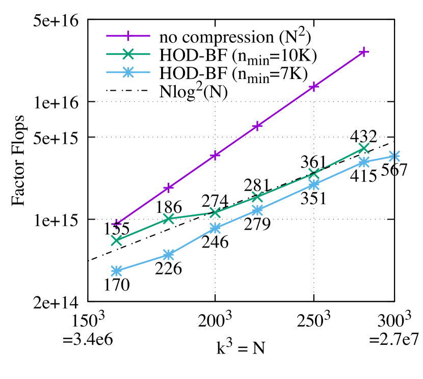
(a)

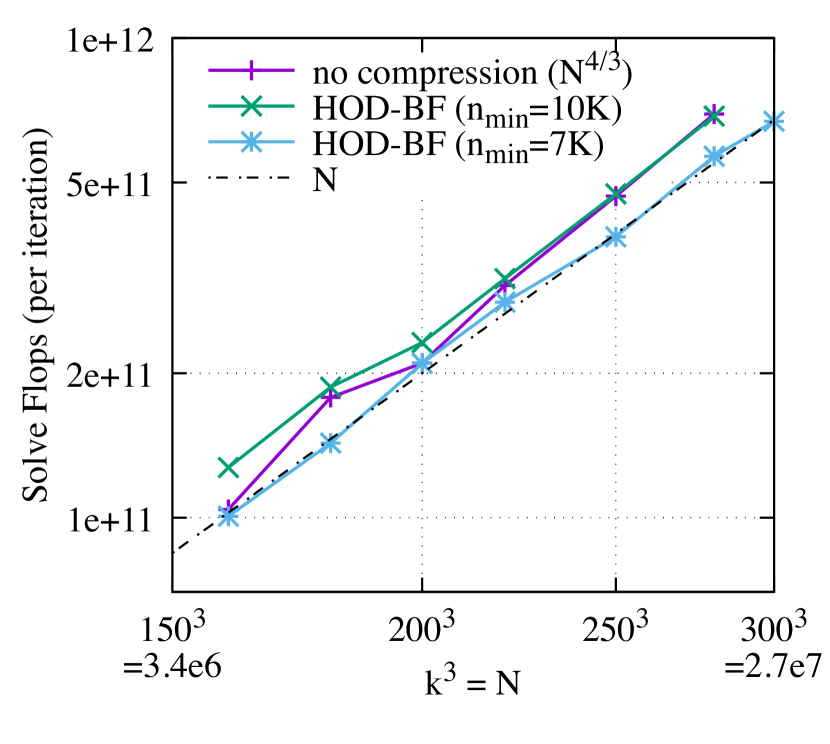
(b)

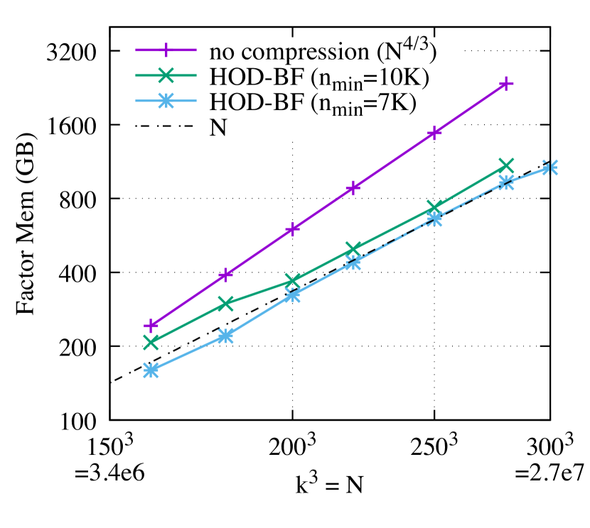
(c)

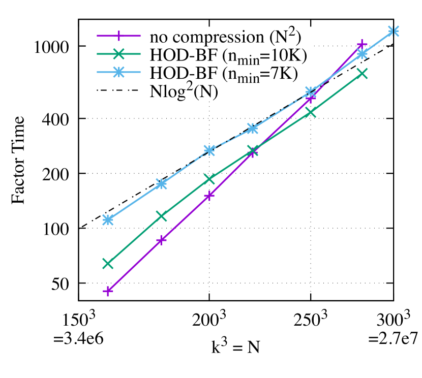
(d)

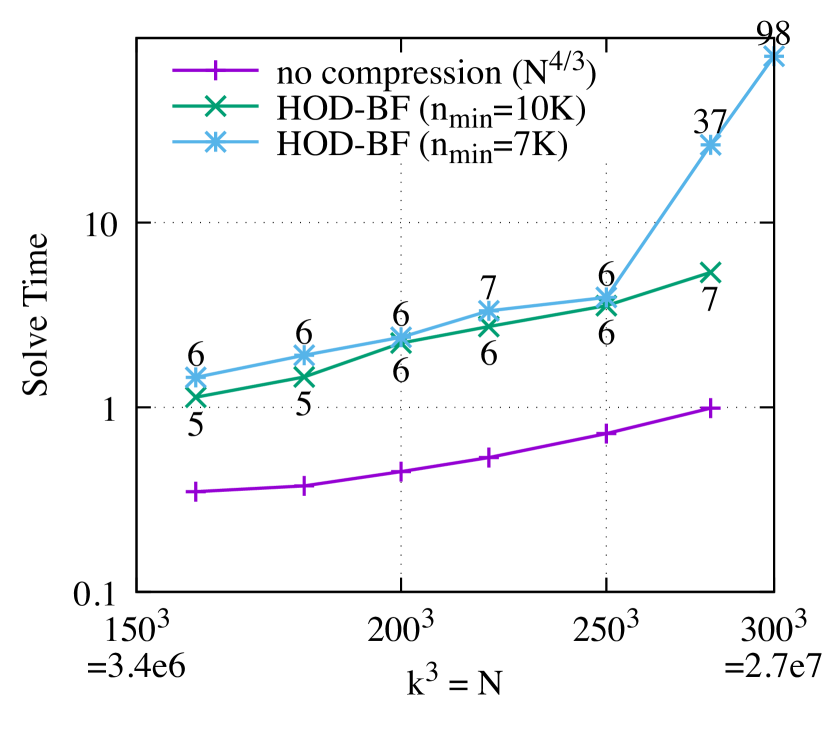
(e)

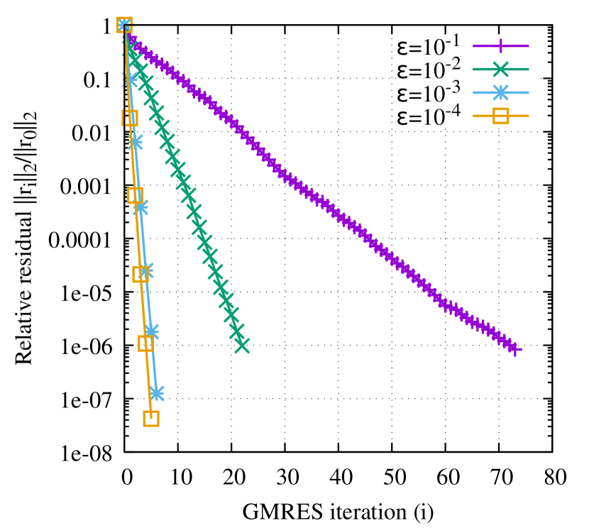
(f)

Figure 6: Results for high frequency 3D Helmholtz using the exact solver with iterative refinement and the HOD-BF($10^{-3}$) multifrontal solver with GMRES. (a) Flop counts for factorization. The maximum ranks are shown at every datapoint of HOD-BF. (b) Flop counts for solve per iteration in GMRES. (c) Memory usage for the factors (not the peak working memory). (d) CPU time for factorization. (e) CPU time for solve. The number of GMRES iterations are shown at every datapoint of HOD-BF. (f) GMRES convergence for $k=200$, with different compression tolerances $\varepsilon$.

Heterogeneous media

Here we use the Marmousi2 [40] P-wave velocity model for $v({\bf x})$, and set $\rho({\bf x})=1$kg/m³, $q({\bf x})=10^{4}$. We generate a $174\times 500$ grid in the x-z plane using the Marmousi2 model and duplicate the model 200 times in the y direction, yielding a mesh of $190\times 216\times 516$ with $N=21,\!176,\!640$ and grid spacing 20m including the PMLs (see Fig. 7). We set the frequency to $\omega=20\pi$ corresponding to 7.5 grid points per miminum wavelength. The real part of the pressure field, induced by a point source located at the domain center, is computed by the proposed HOD-BF multifrontal solver with 32 compute nodes and plotted in Fig. 7. The difference between the pressure field, computed by the HOD-BF multifrontal solver with and without GMRES is also plotted. When $\varepsilon=10^{-6}$, the HOD-BF multifrontal solver can also serve as a good direct solver (without GMRES). The technical data with different compression tolerances and switching levels is listed in Table 3 and compared with exact and HSS multifrontal solvers. Significant flop and memory compression ratios have been observed. Note that there is a trade-off between the factor and solve times when using different tolerances and switching levels.

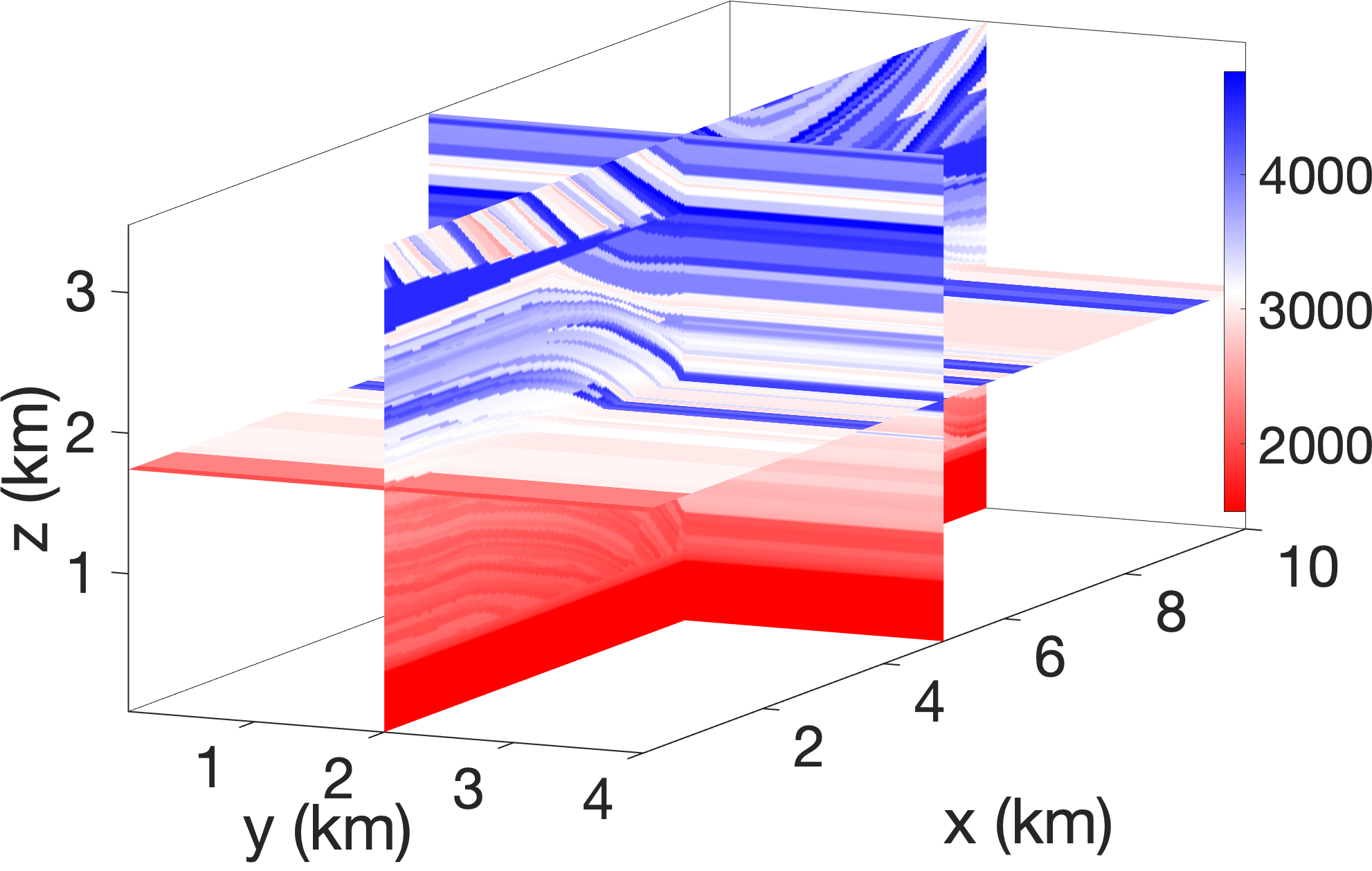
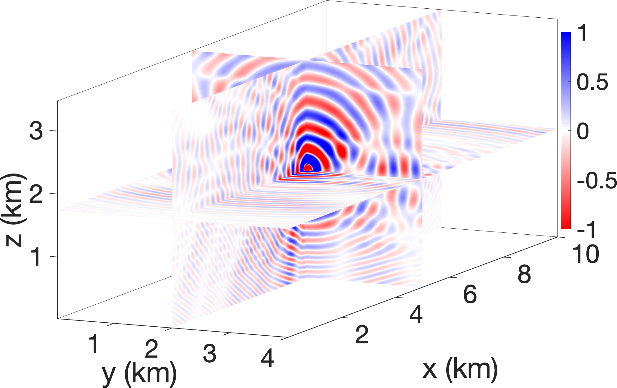
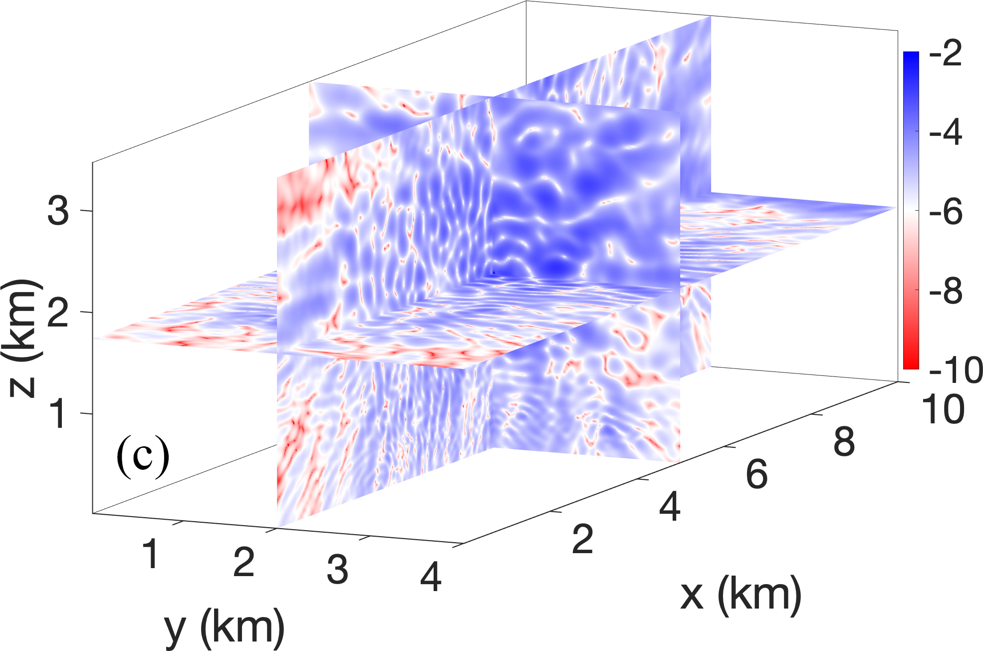
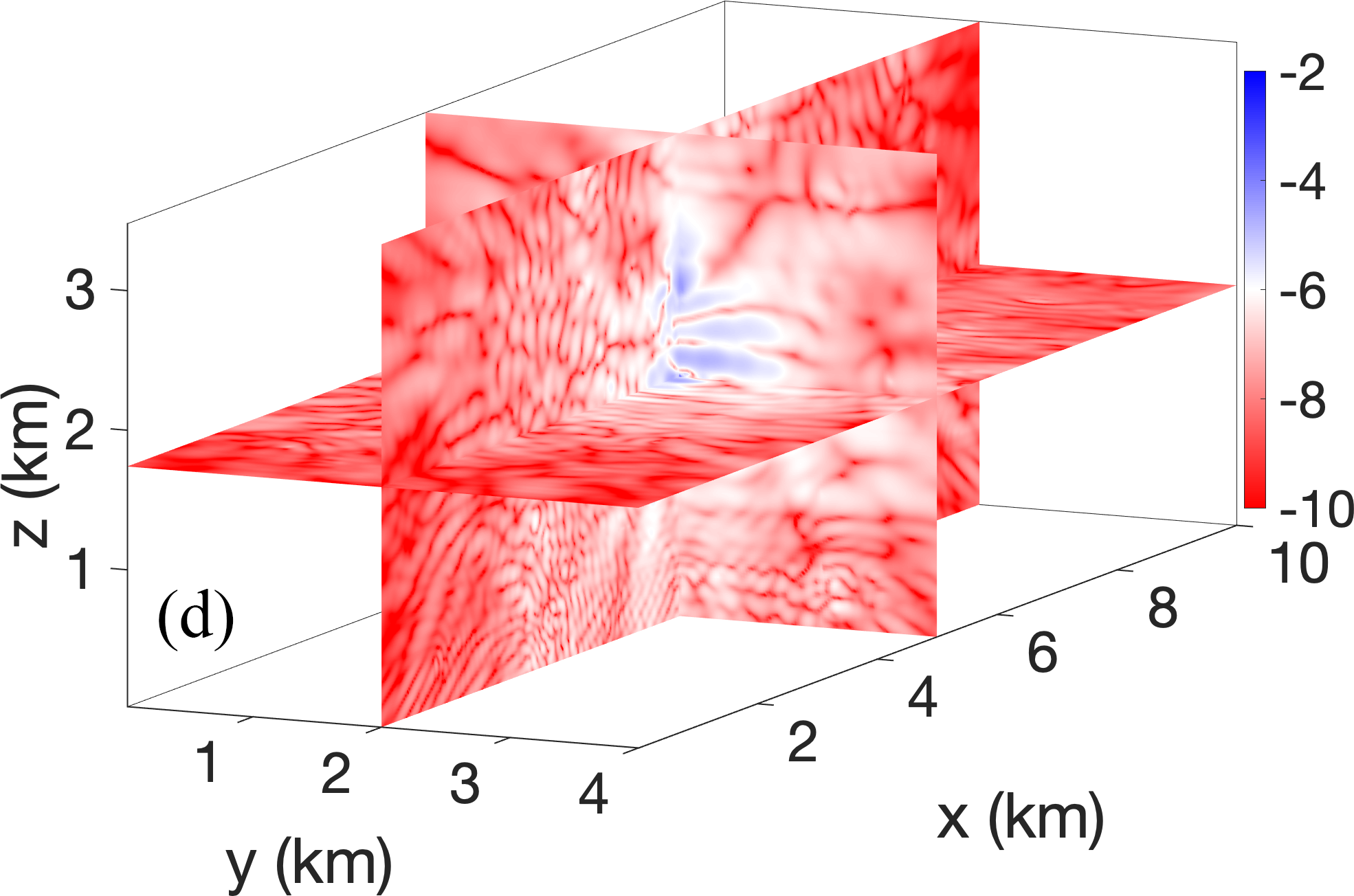
Figure 7: (a) 3D extension of the Marmousi2 velocity model, (b) the real part of the pressure wave field $p({\bf r})$ excited by a point source at the domain center computed by the HOD-BF($10^{-4}$) multifrontal solver with GMRES, (c) difference in $|p({\bf r})|$ of log scale computed by HOD-BF($10^{-4}$) with and without GMRES, (d) difference in $|p({\bf r})|$ of log scale computed by HOD-BF($10^{-6}$) with and without GMRES. We use 32 compute nodes.

Solver	Exact	HSS	HOD-BF	HOD-BF	HOD-BF	HOD-BF
$\varepsilon$	-	$10^{-3}$	$10^{-3}$	$10^{-3}$	$10^{-4}$	$10^{-6}$
$n_{\rm min}$	-	75K	38.5K	75K	75K	75K
Compressed fronts	-	143	435	143	143	143
Dense fronts	2,102,917	2,102,774	2,102,482	2,102,774	2,102,774	2,102,774
Factor time (sec)	660	1575	1037	674	1049	1657
Factor flops ($10^{15}$)	17.8	7.33	2.19	2.17	2.71	4.51
Flop Compression (%)	100	41.2	12.3	12.2	15.2	25.3
Memory ($10^{3}$ GB)	1.97	1.01	0.58	0.77	0.8	0.87
Mem Compression (%)	100	51.08	29.91	39.3	40.7	44.6
Maximum rank	-	4105	549	492	608	824
GMRES iterations	0	6	59	63	12	3
Solve flops ($10^{12}$)	0.55	3.91	23.3	34.6	6.97	2.30
Solve time (sec)	0.9	11.8	48.7	52.8	11.0	4.1

Table 3: Data for applying HOD-BF, HSS and exact multifrontal solvers to Eq. 14 with the Marmousi2 velocity model. We use 32 compute nodes.

6.2 Indefinite Maxwell

We solve the electromagnetics problem corresponding to the second order Maxwell equation, $\nabla\times\nabla\times\mathbf{E}-\Omega^{2}\mathbf{E}=\mathbf{f}$, which is given in the weak formulation as $\left(\nabla\times\mathbf{E},\nabla\times\mathbf{E^{\prime}}\right)-\left(\Omega^{2}\mathbf{E},\mathbf{E^{\prime}}\right)=\left(\mathbf{f},\mathbf{E^{\prime}}\right)$ with a testing function $\mathbf{E^{\prime}}$. Here it is assumed a given tangential field as boundary condition for $\mathbf{E}$. More specifically, $\mathbf{f}(\mathbf{x})=(\kappa^{2}-\Omega^{2})(\sin(\kappa x_{2}),\sin(\kappa x_{3}),\sin(\kappa x_{1}))$ on the domain boundaries. For large wavenumber $\Omega$, the problem is highly indefinite and hard to precondition, so typically a direct solver is used. We discretize the weak form with first order Nédélec elements using MFEM [6]. We use a uniform tetrahedral finite element mesh on a unit cube, resulting in a linear system of size $14,\!827,\!904$ and approximately 24 points per wavelength. The results for $\Omega=32$ and $\kappa=\Omega/1.05$ are shown in Fig. 8.

Solver	Exact	HOD-BF
$\varepsilon$	-	$10^{-5}$
$n_{min}$	-	15K
Compressed fronts	0	6
Dense fronts	3,773,221	3,773,215
Factor time (sec)	301.34	379.50
Factor flops ($10^{15}$)	2.13	1.28
Flop Compr. (%)	100	60.1
Memory (GB)	541	426
Mem Compr. (%)	100	78.8
Max rank/front size	-	955 / 78203
GMRES its.	1	21
Solve flops ($10^{12}$)	1.18	2.45
Solve time (sec)	1.09	18.98

Figure 8: Left: Data for applying the exact and HOD-BF($10^{-5}$) solvers to the indefinite Maxwell equation. Right: Magnitude of computed solution $E$. We use $16$ compute nodes.

6.3 3D Poisson

We solve the Poisson equation on a regular 3D $k^{3}$ mesh using $64$ compute nodes, with 4 MPI ranks per node and 8 OpenMP threads per MPI process. Fig. 9 shows the factor flop and time, solve flop and time, and factor memory using HOD-BF, HSS and exact multifrontal solvers. The HSS multifrontal solver [54, 19], is also implemented in STRUMPACK. The maximum ranks and iteration counts are also shown in Fig. 9(a) and Fig. 9(e), respectively. HOD-BF outperforms exact solver and HSS solver respectively for $k>200$ and $k>300$ in terms of factor time, due to quasi-linear complexities predicted by Table 1. Fig. 9(f) shows that the maximum ranks in the HOD-BF representation, as a function of the size $n$ of the root front, remain much smaller than those in HSS. Note the agreement with Table 1, which predicts $\mathcal{O}(n^{1/2})$ and $\mathcal{O}(n^{1/4})$ for HSS and HOD-BF respectively. For the $425^{3}$ problem, the top separator is a $425\times 425$ plane, corresponding to a $180,\!625^{2}$ frontal matrix. The largest front is found at the next level, $\ell=1$, and is $270,\!938^{2}$ ($=425\times 425/2+425\times 425$). Using HSS, this front is compressed to $2.49\%$ of the dense storage with a maximum off-diagonal rank of $2856$, while HOD-BF compresses this front to $0.38\%$ with a maximum rank of $120$.

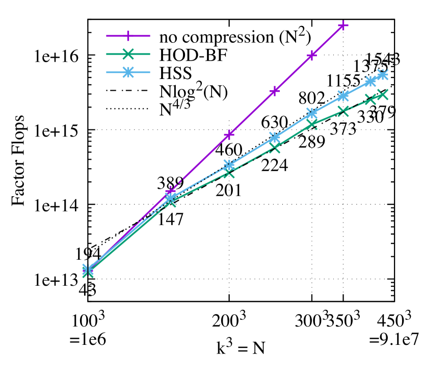
(a)

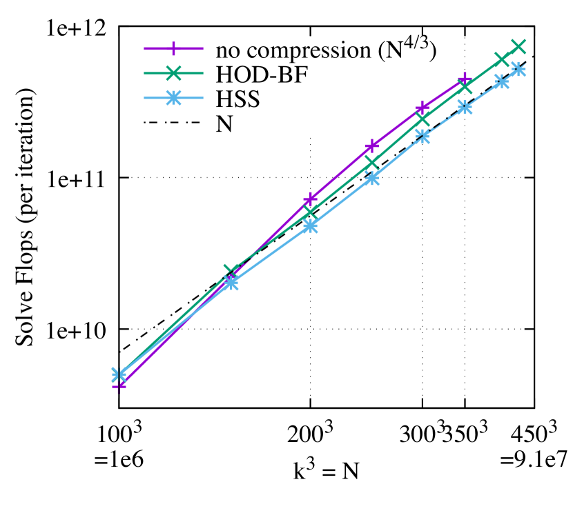
(b)

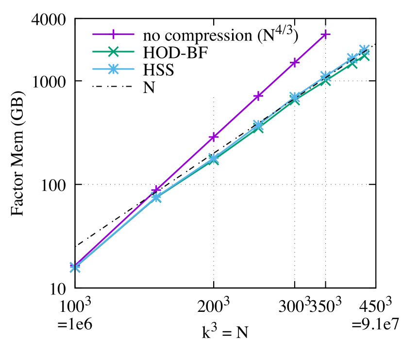
(c)

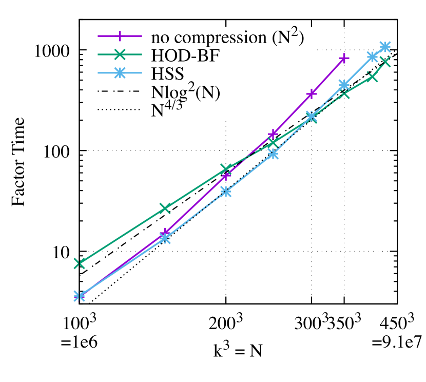
(d)

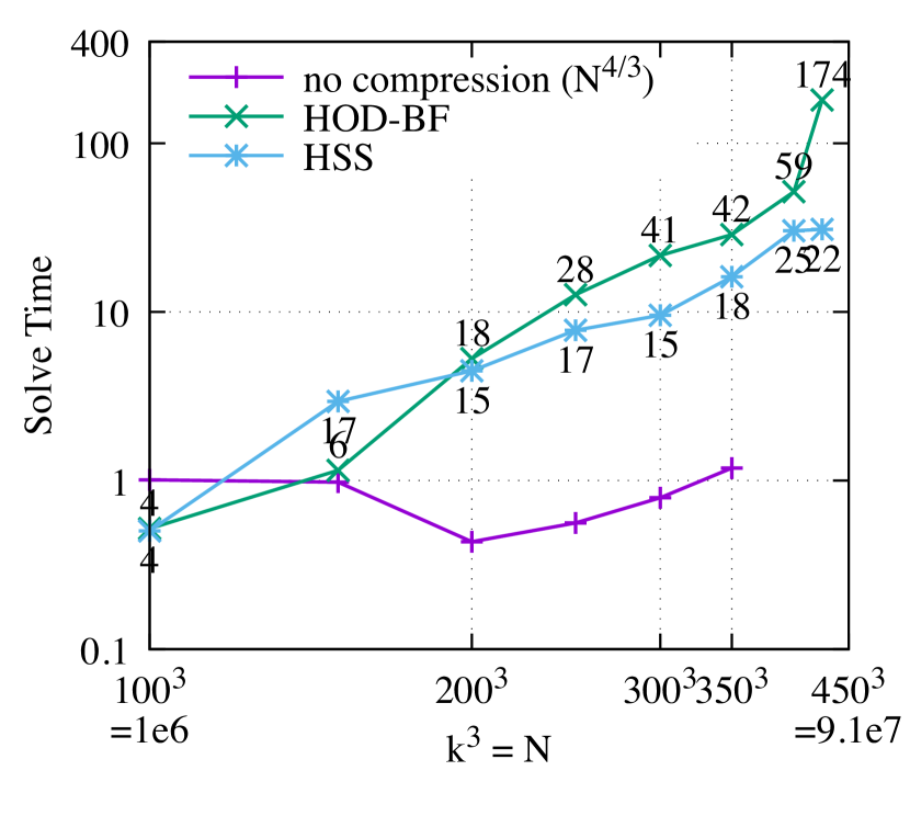
(e)

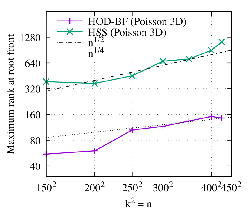
(f)

Figure 9: Results for 3D Poisson using the exact solver with iterative refinement, the HOD-BF multifrontal solver with GMRES and compression tolerance $\varepsilon=10^{-3}$, and the HSS multifrontal solver with GMRES and compression tolerance $\varepsilon=10^{-2}$. (a) Flop counts for factorization. The maximum ranks are shown at every datapoint of HOD-BF. (b) Flop counts for solve per iteration in GMRES. (c) Memory usage for the factors (not the peak working memory). (d) CPU time for factorization. (e) CPU time for solve. The number of GMRES iterations are shown at every datapoint of HOD-BF. (f) The maximum ranks encountered in the HSS or HOD-BF representations at the root front.

7 Conclusion

This paper presents a fast multifrontal sparse solver for high-frequency wave equations. The solver leverages the butterfly algorithm and its hierarchical matrix extension, HOD-BF, to compress large frontal matrices. The butterfly representation is computed via fast entry evaluation based on the graph distance, and factorized with randomized matrix-vector multiplication-based algorithms. The resulting solver can attain quasi-linear computation and memory complexity when applied to high-frequency Helmholtz and Maxwell equations. Similar complexities have been analyzed and observed for Poisson equations as well. The code is made publicly available as an effort to integrate the dense solver package ButterflyPACK into the sparse solver package STRUMPACK. To further reduce the overall number of operations and especially the factorization time, a hybrid multifrontal solver which employs HOD-BF for large sized fronts, and BLR or HSS for medium sized fronts is under development.

References

- [1] Sivaram Ambikasaran and Eric Darve. An fast direct solver for partial hierarchically semi-separable matrices. SIAM J. Sci. Comput, 57(3):477–501, December 2013.
- [2] Patrick Amestoy, Cleve Ashcraft, Olivier Boiteau, Alfredo Buttari, Jean-Yves L’Excellent, and Clément Weisbecker. Improving multifrontal methods by means of block low-rank representations. SIAM J. Sci. Comput., 37(3):A1451–A1474, 2015.
- [3] Patrick R. Amestoy, Alfredo Buttari, Jean-Yves L’Excellent, and Theo Mary. Performance and scalability of the block low-rank multifrontal factorization on multicore architectures. ACM Trans. Math. Softw., 45(1), February 2019.
- [4] Patrick R. Amestoy, Alfredo Buttari, Jean-Yves L’Excellent, and Theo A. Mary. Bridging the gap between flat and hierarchical low-rank matrix formats: The multilevel block low-rank format. SIAM Journal on Scientific Computing, 41(3):A1414–A1442, 2019.
- [5] Amirhossein Aminfar, Sivaram Ambikasaran, and Eric Darve. A fast block low-rank dense solver with applications to finite-element matrices. J. Comput. Phys., 304:170–188, 2016.
- [6] Robert Anderson, Julian Andrej, Andrew Barker, Jamie Bramwell, Jean-Sylvain Camier, Jakub Cerveny, Veselin Dobrev, Yohann Dudouit, Aaron Fisher, Tzanio Kolev, et al. MFEM: a modular finite element methods library. arXiv preprint arXiv:1911.09220, 2019.
- [7] Ariful Azad, Aydın Buluc, Xiaoye S. Li, Xinliang Wang, and Johannes Langguth. A distributed-memory algorithm for computing a heavy-weight perfect matching on bipartite graphs. SIAM J. Scientific Computing, 2020 (to appear).
- [8] James Bremer, Ze Chen, and Haizhao Yang. Rapid Application of the Spherical Harmonic Transform via Interpolative Decomposition Butterfly Factorization. arXiv preprint arXiv:2004.11346, 2020.
- [9] Ovidio M. Bucci and Giorgio Franceschetti. On the spatial bandwidth of scattered fields. IEEE Trans. Antennas Propag., 35(12):1445–1455, 1987.
- [10] Steffen Börm. Directional -matrix compression for high-frequency problems. Numer. Linear Algebra Appl., 24(6):e2112, 2017.
- [11] Emmanuel Candès, Laurent Demanet, and Lexing Ying. A fast butterfly algorithm for the computation of Fourier integral operators. Multiscale Model. Sim., 7(4):1727–1750, 2009.
- [12] Jeffrey N. Chadwick and David S. Bindel. An efficient solver for sparse linear systems based on rank-structured Cholesky factorization. arXiv preprint arXiv:1507.05593, 2015.
- [13] Shiv Chandrasekaran, Patrick Dewilde, Ming Gu, and Naveen Somasunderam. On the numerical rank of the off-diagonal blocks of Schur complements of discretized elliptic PDEs. SIAM Journal on Matrix Anal. Appl., 31:2261–2290, 2010.
- [14] Timothy A. Davis, Sivasankaran Rajamanickam, and Wissam M. Sid-Lakhdar. A survey of direct methods for sparse linear systems. Acta Numer., 25:383–566, 2016.
- [15] Iain S Duff and Jacko Koster. The design and use of algorithms for permuting large entries to the diagonal of sparse matrices. SIAM J MATRIX ANAL A., 20(4):889–901, 1999.
- [16] Iain S Duff and John Ker Reid. The multifrontal solution of indefinite sparse symmetric linear. ACM Trans. Math. Softw., 9(3):302–325, 1983.
- [17] I.S. Duff, A.M. Erisman, and J.K. Reid. Direct Methods for Sparse Matrices, Second Edition. Oxford University Press, London, 2017.
- [18] Björn Engquist and Hongkai Zhao. Approximate separability of the Green’s function of the Helmholtz equation in the high frequency limit. Commun Pur. Appl. Math., 71(11):2220–2274, 2018.
- [19] Pieter Ghysels, Xiaoye Sherry Li, Christopher Gorman, and François-Henry Rouet. A robust parallel preconditioner for indefinite systems using hierarchical matrices and randomized sampling. In 2017 IEEE International Parallel and Distributed Processing Symposium (IPDPS), pages 897–906. IEEE, 2017.
- [20] Lars Grasedyck and Wolfgang Hackbusch. Construction and arithmetics of H-matrices. Computing, 70(4):295–334, 2003.
- [21] Han Guo, Jun Hu, and Eric Michielssen. On MLMDA/butterfly compressibility of inverse integral operators. IEEE Antennas Wirel. Propag. Lett., 12:31–34, 2013.
- [22] Han Guo, Yang Liu, Jun Hu, and Eric Michielssen. A butterfly-based direct integral-equation solver using hierarchical LU factorization for analyzing scattering from electrically large conducting objects. IEEE Trans. Antennas Propag., 65(9):4742–4750, 2017.
- [23] Han Guo, Yang Liu, Jun Hu, and Eric Michielssen. A butterfly-based direct integral-equation solver using hierarchical LU factorization for analyzing scattering from electrically large conducting objects. IEEE Trans. Antennas Propag., 65(9):4742–4750, 2017.
- [24] Han Guo, Yang Liu, Jun Hu, and Eric Michielssen. A butterfly-based direct solver using hierarchical LU factorization for Poggio-Miller-Chang-Harrington-Wu-Tsai equations. Microw Opt Technol Lett., 60:1381–1387, 2018.
- [25] Wolfgang Hackbusch. A sparse matrix arithmetic based on -matrices. Part I: Introduction to -matrices. Computing, 62(2):89–108, April 1999.
- [26] Wolfgang Hackbusch and Steffen Börm. Data-sparse approximation by adaptive -matrices. Computing, 69(1):1–35, September 2002.
- [27] Wolfgang Hackbusch, Boris N Khoromskij, and Ronald Kriemann. Hierarchical matrices based on a weak admissibility criterion. Computing, 73(3):207–243, 2004.
- [28] William W. Hager. Updating the inverse of a matrix. SIAM Review, 31(2):221–239, 1989.
- [29] Pascal Hénon, Pierre Ramet, and Jean Roman. PaStiX: a High-Performance Parallel Direct Solver for Sparse Symmetric Positive Definite Systems. Parallel Computing, 28(2):301–321, 2002.
- [30] Kenneth L. Ho and Leslie Greengard. A fast direct solver for structured linear systems by recursive skeletonization. SIAM J. Sci. Comput., 34(5):A2507–A2532, 2012.
- [31] Kenneth L Ho and Lexing Ying. Hierarchical interpolative factorization for elliptic operators: differential equations. Communications on Pure and Applied Mathematics, 69(8):1415–1451, 2016.
- [32] George Karypis and Vipin Kumar. A fast and high quality multilevel scheme for partitioning irregular graphs. SIAM J. Sci. Comput., 20(1):359–392, 1998.
- [33] Yingzhou Li and Haizhao Yang. Interpolative butterfly factorization. SIAM J. Sci. Comput., 39(2):A503–A531, 2017.
- [34] Yingzhou Li, Haizhao Yang, Eileen R Martin, Kenneth L Ho, and Lexing Ying. Butterfly factorization. Multiscale Model. Sim., 13(2):714–732, 2015.
- [35] Yingzhou Li and Lexing Ying. Distributed-memory hierarchical interpolative factorization. Research in the Mathematical Sciences, 4(1):12, 2017.
- [36] J. W. H. Liu. The multifrontal method for sparse matrix solution: theory and practice. SIAM Review, 34(1):82–109, March 1992.
- [37] Yang Liu, Han Guo, and Eric Michielssen. An HSS matrix-inspired butterfly-based direct solver for analyzing scattering from two-dimensional objects. IEEE Antennas Wirel. Propag. Lett., 16:1179–1183, 2017.
- [38] Yang Liu, Xin Xing, Han Guo, Eric Michielssen, Pieter Ghysels, and Xiaoye Sherry Li. Butterfly factorization via randomized matrix-vector multiplications. arXiv preprint arXiv:2002.03400, 2020.
- [39] Yang Liu and Haizhao Yang. A hierarchical butterfly LU preconditioner for two-dimensional electromagnetic scattering problems involving open surfaces. J. Comput. Phys., 401:109014, 2020.
- [40] Gary S. Martin, Robert Wiley, and Kurt J. Marfurt. Marmousi2: An elastic upgrade for Marmousi. The Leading Edge, 25(2):156–166, 2006.
- [41] Eric Michielssen and Amir Boag. Multilevel evaluation of electromagnetic fields for the rapid solution of scattering problems. Microw Opt Technol Lett., 7(17):790–795, 1994.
- [42] Eric Michielssen and Amir Boag. A multilevel matrix decomposition algorithm for analyzing scattering from large structures. IEEE Trans. Antennas Propag., 44(8):1086–1093, 1996.
- [43] Richard Nies and Matthias Hoelzl. Testing performance with and without block low rank compression in MUMPS and the new PaStiX 6.0 for JOREK nonlinear MHD simulations. arXiv:1907.13442, 2019.
- [44] Michael O’Neil, Franco Woolfe, and Vladimir Rokhlin. An algorithm for the rapid evaluation of special function transforms. Appl. Comput. Harmon. A., 28(2):203 – 226, 2010. Special Issue on Continuous Wavelet Transform in Memory of Jean Morlet, Part I.
- [45] Stéphane Operto, Jean Virieux, Patrick Amestoy, Jean-Yves L’Excellent, Luc Giraud, and Hafedh Ben Hadj Ali. 3D finite-difference frequency-domain modeling of visco-acoustic wave propagation using a massively parallel direct solver: A feasibility study. Geophysics, 72(5):SM195–SM211, 2007.
- [46] Qiyuan Pang, Kenneth L. Ho, and Haizhao Yang. Interpolative decomposition butterfly factorization. SIAM J. Sci. Comput., 42(2):A1097–A1115, 2020.
- [47] Hadi Pouransari, Pieter Coulier, and Eric Darve. Fast hierarchical solvers for sparse matrices using extended sparsification and low-rank approximation. SIAM J. Sci. Comput., 39(3):A797–A830, 2017.
- [48] John Shaeffer. Direct Solve of Electrically Large Integral Equations for Problem Sizes to 1 M Unknowns. IEEE Trans. Antennas Propag., 56(8):2306–2313, 2008.
- [49] STRUMPACK: STRUctured Matrices PACKages. http://portal.nersc.gov/project/sparse/strumpack/.
- [50] Matthias Taus, Leonardo Zepeda-Núñez, Russell J Hewett, and Laurent Demanet. L-Sweeps: A scalable, parallel preconditioner for the high-frequency Helmholtz equation, 2019.
- [51] Mark Tygert. Fast algorithms for spherical harmonic expansions, III. J. Comput. Phys., 229(18):6181 – 6192, 2010.
- [52] Raf Vandebril, Marc Van Barel, Gene Golub, and Nicola Mastronardi. A bibliography on semiseparable matrices. Calcolo, 42(3-4):249–270, 2005.
- [53] Shen Wang, Xiaoye S. Li, François-Henry Rouet, Jianlin Xia, and Maarten V. De Hoop. A Parallel Geometric Multifrontal Solver Using Hierarchically Semiseparable Structure. ACM Trans. Math. Softw., 42(3), May 2016.
- [54] Jianlin Xia. Randomized sparse direct solvers. SIAM Journal on Matrix Anal. Appl., 34:197–227, 2013.
- [55] Haizhao Yang. A unified framework for oscillatory integral transforms: When to use NUFFT or butterfly factorization? J. Comput. Phys., 388:103 – 122, 2019.
- [56] Lexing Ying. Sparse Fourier Transform via Butterfly Algorithm. SIAM J. Sci. Comput., 31(3):1678–1694, 2009.
- [57] Lexing Ying. Directional preconditioner for 2D high frequency obstacle scattering. Multiscale Model. Sim., 13(3):829–846, 2015.
- [58] Bangda Zhou and Dan Jiao. Direct Finite-Element Solver of Linear Complexity for Large-Scale 3-D Electromagnetic Analysis and Circuit Extraction. IEEE T. MICROW. THEORY, 63(10):3066–3080, 2015.