All in the Exponential Family:
Bregman Duality in Thermodynamic Variational Inference

Abstract

The recently proposed Thermodynamic Variational Objective (tvo) leverages thermodynamic integration to provide a family of variational inference objectives, which both tighten and generalize the ubiquitous Evidence Lower Bound (elbo). However, the tightness of tvo bounds was not previously known, an expensive grid search was used to choose a “schedule” of intermediate distributions, and model learning suffered with ostensibly tighter bounds. In this work, we propose an exponential family interpretation of the geometric mixture curve underlying the tvo and various path sampling methods, which allows us to characterize the gap in tvo likelihood bounds as a sum of KL divergences. We propose to choose intermediate distributions using equal spacing in the moment parameters of our exponential family, which matches grid search performance and allows the schedule to adaptively update over the course of training. Finally, we derive a doubly reparameterized gradient estimator which improves model learning and allows the tvo to benefit from more refined bounds. To further contextualize our contributions, we provide a unified framework for understanding thermodynamic integration and the tvo using Taylor series remainders.

Proof.

1 Introduction

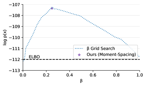
Figure 1: The original tvo paper recommended using two partition points, with a single intermediate $\beta_{1}$ in addition to the elbo at $\beta_{0}=0$. We report test $\log{p_{\theta}(\operatorname{\mathbf{x}})}$ values from training a separate vae at each $\beta_{1}$, but this grid search is prohibitively expensive in practice. Our moment-spacing schedule is an adaptive method for choosing $\beta$ points, which yields near-optimal performance on Omniglot and provides notable improvement over the elbo.

Modern variational inference (vi) techniques are able to jointly perform maximum likelihood parameter estimation and approximate posterior inference using stochastic gradient ascent (Kingma & Welling, 2013; Rezende et al., 2014). Commonly, this is done by optimizing a tractable bound to the marginal log likelihood $\log p_{\theta}(\operatorname{\mathbf{x}})=\int p_{\theta}(\operatorname{\mathbf{x}},\operatorname{\mathbf{z}})\operatorname{d\mathbf{z}}$, obtained by introducing a divergence $D[{q_{\phi}(\operatorname{\mathbf{z}}|\operatorname{\mathbf{x}})}||{p_{\theta}(\operatorname{\mathbf{z}}|\operatorname{\mathbf{x}})}]$ between the variational distribution ${q_{\phi}(\operatorname{\mathbf{z}}|\operatorname{\mathbf{x}})}$ and true posterior ${p_{\theta}(\operatorname{\mathbf{z}}|\operatorname{\mathbf{x}})}$ (Blei et al., 2017; Li & Turner, 2016; Dieng et al., 2017; Cremer et al., 2017; Wang et al., 2018).

The recent Thermodynamic Variational Objective (tvo) (Masrani et al., 2019) reframes likelihood estimation in terms of numerical integration along a geometric mixture path connecting ${q_{\phi}(\operatorname{\mathbf{z}}|\operatorname{\mathbf{x}})}$ and ${p_{\theta}(\operatorname{\mathbf{z}}|\operatorname{\mathbf{x}})}$. This perspective yields a natural family of lower and upper bounds via Riemann sum approximations, with the elbo appearing as a single-term lower bound and wake-sleep (ws) $\phi$ update corresponding to the simplest upper bound. The tvo generalizes these objectives by using a $K$-term Riemann sum to obtain tighter bounds on marginal likelihood. We refer to the discrete partition $\{\beta_{k}\}_{k=0}^{K}$ used to construct this estimator as an ‘integration schedule.’

However, the gaps associated with these intermediate bounds was not previously known, an important roadblock to understanding the objective. Further, the tvo was limited by a grid search procedure for choosing the integration schedule. While tvo bounds should become tighter with more refined partitions, Masrani et al. (2019) actually observe deteriorating performance in practice with high $K$.

Our central contribution is an exponential family interpretation of the geometric mixture curve underlying the tvo and various path sampling methods (Gelman & Meng, 1998; Neal, 2001). Using the Bregman divergences associated with this family, we characterize the gaps in the tvo upper and lower bounds as the sum of KL divergences along a given path, resolving this open question about the tvo.

Further, we propose to choose intermediate distributions in the tvo based on the ‘moment-averaged’ path of Grosse et al. (2013), which arises naturally from the dual parameterization of our exponential family. This scheduling scheme was originally proposed in the context of annealed importance sampling (ais), where additional sampling procedures may be required to even approximate it. We provide an efficient implementation for the tvo setting, which allows the choice of $\beta$ to adapt to the shape of the integrand and degree of posterior mismatch throughout training.

In Figure 1, we observe that this flexible schedule yields near-optimal performance compared to grid search for a single intermediate distribution, so that the tvo can significantly improve upon the elbo for minimal additional cost. However, our moments scheduler can still suffer the previously observed performance degradation as the number of intermediate distributions increases. As a final contribution, we propose a doubly reparameterized gradient estimator for the tvo, which we show can avoid this undesirable behavior and improve overall performance in continuous models.

Our exponential family analysis may be of wider interest given the prevalence of Markov Chain Monte Carlo (mcmc) techniques utilizing geometric mixture paths (Neal, 1996, 2001; Grosse et al., 2016; Syed et al., 2019; Huang et al., 2020). To this end, we also present a framework for understanding thermodynamic integration (ti) (Ogata, 1989) and the tvo using Taylor series remainders, which clarifies that the tvo is a first-order objective and provides geometric intuition for several results from Grosse et al. (2013). We hope these connections can help open new avenues for analysis at the intersection of mcmc, vi, and statistical physics.

Figure 2: The tvo is a K-term Riemann sum approximation of $\log{p_{\theta}(\operatorname{\mathbf{x}})}$, which can be expressed as a scalar integral over the unit interval in (6) and on the right. The $\operatorname{\textsc{elbo}}$ is a single-term left Riemann approximation of the same integral using the point $\beta=0$ with $\pi_{0}={q_{\phi}(\operatorname{\mathbf{z}}|\operatorname{\mathbf{x}})}$. Note that the integrand is negative in practice, but shown as positive for interpretability.

2 Background

2.1 Thermodynamic Integration

Thermodynamic integration (ti) is a technique from statistical physics, which frames estimating ratios of partition functions as a one-dimensional integration problem. Commonly, this integral is taken over $\beta\in[0,1]$, which parameterizes a path of geometric mixtures between a base distribution $\pi_{0}$, and a target distribution $\pi_{1}$ (Gelman & Meng, 1998)

$$\pi_{\beta}(\operatorname{\mathbf{z}}):=\frac{\tilde{\pi}_{\beta}(\operatorname{\mathbf{z}})}{\int\tilde{\pi}_{\beta}(\operatorname{\mathbf{z}})\,d\operatorname{\mathbf{z}}}=\frac{\pi_{0}^{1-\beta}(\operatorname{\mathbf{z}})\pi_{1}^{\beta}(\operatorname{\mathbf{z}})}{Z_{\beta}}\,.$$ (1)

The insight of ti is to recognize that, while the log partition function is intractable, its derivative can be written as an expectation that may be estimated using sampling or simulation techniques (Neal, 2001; Habeck, 2017)

$$\nabla_{\beta}\log Z_{\beta} =\operatorname{\mathbb{E}}_{{\pi_{\beta}}}\left[\log\frac{\pi_{1}(\operatorname{\mathbf{z}})}{\pi_{0}(\operatorname{\mathbf{z}})}\right]\,.$$ (2)

In Sec. 3, we will see that this identity arises from an interpretation of the geometric mixture curve Equation 1 as an exponential family. Applying this within the fundamental theorem of calculus,

$$\log Z_{1}-\log Z_{0} =\int_{0}^{1}\nabla_{\beta}\log Z_{\beta}\,d\beta$$ (3)

$$=\int_{0}^{1}\operatorname{\mathbb{E}}_{{\pi_{\beta}}}\left[\log\frac{\pi_{1}(\operatorname{\mathbf{z}})}{\pi_{0}(\operatorname{\mathbf{z}})}\right]d\beta.$$ (4)

While (3) holds for any choice of path parameterized by $\beta$, we can construct efficient estimators of the integrand in (4) and estimate the partition function ratio $\log Z_{1}/Z_{0}$ using numerical integration techniques.

2.2 The Thermodynamic Variational Objective

The tvo (Masrani et al., 2019) uses ti in the context of variational inference to provide natural upper and lower bounds on the log evidence, which can then be used as objectives for training latent variable models. In particular, the geometric mixture path interpolates between the approximate posterior ${q_{\phi}(\operatorname{\mathbf{z}}|\operatorname{\mathbf{x}})}$ and the joint generative model ${p_{\theta}(\operatorname{\mathbf{x}},\operatorname{\mathbf{z}})}$

$$\operatorname{\pi_{\beta}(\operatorname{\mathbf{z}}|\operatorname{\mathbf{x}})} =\frac{\operatorname{\tilde{\pi}_{\beta}(\operatorname{\mathbf{x}},\operatorname{\mathbf{z}})}}{\int\operatorname{\tilde{\pi}_{\beta}(\operatorname{\mathbf{x}},\operatorname{\mathbf{z}})}\operatorname{d\mathbf{z}}}:=\frac{{q_{\phi}(\operatorname{\mathbf{z}}|\operatorname{\mathbf{x}})}^{1-\beta}{p_{\theta}(\operatorname{\mathbf{x}},\operatorname{\mathbf{z}})}^{\beta}}{Z_{\beta}(\operatorname{\mathbf{x}})}\,.$$ (5)

As distributions over $\operatorname{\mathbf{z}}$, we can identify the endpoints as $\pi_{0}(\operatorname{\mathbf{z}}|\operatorname{\mathbf{x}})={q_{\phi}(\operatorname{\mathbf{z}}|\operatorname{\mathbf{x}})}$ and $\pi_{1}(\operatorname{\mathbf{z}}|\operatorname{\mathbf{x}})={p_{\theta}(\operatorname{\mathbf{z}}|\operatorname{\mathbf{x}})}$, with corresponding normalizing constants $Z_{0}=1$ and $Z_{1}=\int{p_{\theta}(\operatorname{\mathbf{x}},\operatorname{\mathbf{z}})}\,d\operatorname{\mathbf{z}}={p_{\theta}(\operatorname{\mathbf{x}})}$.

Applying ti Equation 3 for this set of log partition functions, Masrani et al. (2019) express the generative model likelihood using a one-dimensional integral over the unit interval

$$\log{p_{\theta}(\operatorname{\mathbf{x}})} =\int_{0}^{1}\operatorname{\mathbb{E}}_{{\pi_{\beta}}}\left[{\log\frac{{p_{\theta}(\operatorname{\mathbf{x}},\operatorname{\mathbf{z}})}}{{q_{\phi}(\operatorname{\mathbf{z}}|\operatorname{\mathbf{x}})}}}\right]d\beta.$$ (6)

The left and right endpoints of this integrand correspond to familiar lower and upper bounds on $\log{p_{\theta}(\operatorname{\mathbf{x}})}$. The evidence lower bound (elbo) occurs at $\beta=0$, while the analogous evidence upper bound (eubo) at $\beta=1$ uses the ‘reverse’ KL divergence and appears in various wake-sleep objectives (ws)  (Hinton et al., 1995; Bornschein & Bengio, 2014)

$$\operatorname{\textsc{elbo}}(\theta,\phi,\operatorname{\mathbf{x}}) =\log{p_{\theta}(\operatorname{\mathbf{x}})}-D_{KL}[q_{\phi}||p_{\theta}]$$ (7)

$$\operatorname{\textsc{eubo}}(\theta,\phi,\operatorname{\mathbf{x}}) =\log{p_{\theta}(\operatorname{\mathbf{x}})}+D_{KL}[p_{\theta}||q_{\phi}].$$ (8)

To arrive at the tvo, a discrete partition schedule is chosen $\mathcal{P}_{\beta}=\{\beta_{k}\}_{k=0}^{K}$ with $\beta_{0}=0$, $\beta_{K}=1$, and $\Delta_{\beta_{k}}=\beta_{k}-\beta_{k-1}.$ The integral in Equation 6 is then approximated using a left or right Riemann sum. Since Masrani et al. (2019) show the integrand is increasing, these approximations yield valid lower and upper bounds on the marginal likelihood

$$\operatorname{\textsc{tvo}}_{\textsc{L}}(\theta,\phi,\operatorname{\mathbf{x}}) :=\sum\limits_{k=1}^{K}\Delta_{\beta_{k}}\operatorname{\mathbb{E}}_{\pi_{\beta_{k-1}}}\bigg{[}{\log\frac{{p_{\theta}(\operatorname{\mathbf{x}},\operatorname{\mathbf{z}})}}{{q_{\phi}(\operatorname{\mathbf{z}}|\operatorname{\mathbf{x}})}}}\bigg{]}$$ (9)

$$\operatorname{\textsc{tvo}}_{\textsc{U}}(\theta,\phi,\operatorname{\mathbf{x}}) :=\sum\limits_{k=1}^{K}\Delta_{\beta_{k}}\operatorname{\mathbb{E}}_{\pi_{\beta_{k}}}\bigg{[}{\log\frac{{p_{\theta}(\operatorname{\mathbf{x}},\operatorname{\mathbf{z}})}}{{q_{\phi}(\operatorname{\mathbf{z}}|\operatorname{\mathbf{x}})}}}\bigg{]}$$ (10)

with

$$\operatorname{\textsc{tvo}}_{\textsc{L}}(\theta,\phi,\operatorname{\mathbf{x}})\leq\log{p_{\theta}(\operatorname{\mathbf{x}})}\leq\operatorname{\textsc{tvo}}_{\textsc{U}}(\theta,\phi,\operatorname{\mathbf{x}}).$$ (11)

The first term of $\operatorname{\textsc{tvo}}_{L}(\theta,\phi,\operatorname{\mathbf{x}})$ corresponds to the $\operatorname{\textsc{elbo}}$, while the last term of $\operatorname{\textsc{tvo}}_{U}(\theta,\phi,\operatorname{\mathbf{x}})$ corresponds to the $\operatorname{\textsc{eubo}}$. Thus, the $\operatorname{\textsc{tvo}}$ generalizes both objectives, with additional partitions leading to tighter bounds on likelihood as visualized in Fig.  2.

Although we consider thermodynamic integration over $0\leq\beta\leq 1$ to approximate $\log{p_{\theta}(\operatorname{\mathbf{x}})}$, note that this integral does not avoid the need for integration over $\operatorname{\mathbf{z}}$ since each intermediate distribution must be normalized. Masrani et al. (2019) propose an efficient, self-normalized importance sampling (snis) scheme with proposal ${q_{\phi}(\operatorname{\mathbf{z}}|\operatorname{\mathbf{x}})}$, so that expectations at any intermediate $\beta$ can be estimated by simply reweighting a single set of importance samples

$$\mathbb{E}_{{\pi_{\beta}}}[\cdot] \approx\sum\limits_{i=1}^{S}\frac{w_{i}^{\beta}}{\sum_{i=1}^{S}w_{s}^{\beta}}\,[\cdot]\,\,\text{where }w_{i}:=\frac{p_{\theta}(\operatorname{\mathbf{x}},\operatorname{\mathbf{z}}_{i})}{q_{\phi}(\operatorname{\mathbf{z}}_{i}|\operatorname{\mathbf{x}})}.$$ (12)

3 Exponential Family Interpretation

We propose a novel exponential family of distributions which, by absorbing both ${p_{\theta}(\operatorname{\mathbf{x}},\operatorname{\mathbf{z}})}$ and ${q_{\phi}(\operatorname{\mathbf{z}}|\operatorname{\mathbf{x}})}$ into the sufficient statistic, corresponds to the geometric mixture path defined in Equation 5. We provide a formal definition in Sec. 3.1, before showing in Sec. 3.2 that several key quantities in the tvo arise from familiar properties of exponential families. In Sec. 4, we leverage the Bregman divergences associated with our exponential family to naturally characterize the gap in tvo bounds as a sum of KL divergences.

3.1 Definition

To match the tvo setting in Equation 5, we consider an exponential family of distributions with natural parameter $\beta$, base measure ${q_{\phi}(\operatorname{\mathbf{z}}|\operatorname{\mathbf{x}})}$, and sufficient statistics equal to the log importance weights as in Equation 9-Equation 10

$${\pi_{\beta}}(\operatorname{\mathbf{z}}|\operatorname{\mathbf{x}}):=\pi_{0}(\operatorname{\mathbf{z}}|\operatorname{\mathbf{x}})\exp\{\,\beta\cdot T(\operatorname{\mathbf{x}},\operatorname{\mathbf{z}})-\psi(\operatorname{\mathbf{x}};\beta)\}$$ (13)

$$\text{where}\,\,T(\operatorname{\mathbf{x}},\operatorname{\mathbf{z}}):={\log\frac{{p_{\theta}(\operatorname{\mathbf{x}},\operatorname{\mathbf{z}})}}{{q_{\phi}(\operatorname{\mathbf{z}}|\operatorname{\mathbf{x}})}}}\quad\pi_{0}(\operatorname{\mathbf{z}}|\operatorname{\mathbf{x}}):={q_{\phi}(\operatorname{\mathbf{z}}|\operatorname{\mathbf{x}})}$$

This induces a log-partition function $\psi(\operatorname{\mathbf{x}};\beta)$, which normalizes over $\operatorname{\mathbf{z}}$ and corresponds to $\log Z_{\beta}(\operatorname{\mathbf{x}})$ in Equation 5

$$\psi(\operatorname{\mathbf{x}};\beta) :=\log\int{q_{\phi}(\operatorname{\mathbf{z}}|\operatorname{\mathbf{x}})}\exp\{\,\beta\,{\log\frac{{p_{\theta}(\operatorname{\mathbf{x}},\operatorname{\mathbf{z}})}}{{q_{\phi}(\operatorname{\mathbf{z}}|\operatorname{\mathbf{x}})}}}\}\operatorname{d\mathbf{z}},$$

$$=\log\int{q_{\phi}(\operatorname{\mathbf{z}}|\operatorname{\mathbf{x}})}^{1-\beta}{p_{\theta}(\operatorname{\mathbf{x}},\operatorname{\mathbf{z}})}^{\beta}\operatorname{d\mathbf{z}}$$ (14)

$$=\log Z_{\beta}(\operatorname{\mathbf{x}}).$$ (15)

The log-partition function will play a key role in our analysis, often written as $\psi(\beta)$ to omit the dependence on $\operatorname{\mathbf{x}}$.

We emphasize that we have made no additional assumptions on ${p_{\theta}(\operatorname{\mathbf{x}},\operatorname{\mathbf{z}})}$ or ${q_{\phi}(\operatorname{\mathbf{z}}|\operatorname{\mathbf{x}})}$, and do not assume they come from exponential families themselves. This ‘higher-order’ exponential family thus maintains full generality and may be constructed between arbitrary distributions.

3.2 TVO using Exponential Families

We now show that a number of key quantities, which were manually derived in the original tvo work, may be directly obtained from our exponential family.

TI Integrates the Mean Parameters

It is well known that the log-partition function $\psi(\beta)$ is convex, with its first (partial) derivative equal to the expectation of the sufficient statistics under $\pi_{\beta}$ (Wainwright & Jordan, 2008).

$$\eta_{\beta}:=\nabla_{\beta}\psi(\beta)=\operatorname{\mathbb{E}}\,[T(\operatorname{\mathbf{x}},\operatorname{\mathbf{z}})]=\operatorname{\mathbb{E}}_{{\pi_{\beta}}}\bigg{[}{\log\frac{{p_{\theta}(\operatorname{\mathbf{x}},\operatorname{\mathbf{z}})}}{{q_{\phi}(\operatorname{\mathbf{z}}|\operatorname{\mathbf{x}})}}}\bigg{]}$$ (16)

This quantity is known as the mean parameter $\eta_{\beta}$, which provides a dual coordinate system for indexing intermediate distributions (Wainwright & Jordan (2008) Sec. 3.5.2). Comparing with Equation 2 and Equation 6, we observe that the ability to trade derivatives of the log-partition function for expectations in ti arises from this property of exponential families.

We may then interpret the tvo as integrating over the mean parameters $\eta_{\beta}=\nabla_{\beta}\log Z_{\beta}$ of our path exponential family, which can be seen by rewriting Equation 3

$$\psi(1)-\psi(0) =\int_{0}^{1}\eta_{\beta}\,d\beta=\int_{0}^{1}\operatorname{\mathbb{E}}_{{\pi_{\beta}}}\bigg{[}{\log\frac{{p_{\theta}(\operatorname{\mathbf{x}},\operatorname{\mathbf{z}})}}{{q_{\phi}(\operatorname{\mathbf{z}}|\operatorname{\mathbf{x}})}}}\bigg{]}d\beta.$$

TVO Likelihood Bounds

The convexity of the log partition function arises from the fact that entries in its matrix of second partial derivatives with respect to the natural parameters correspond to the (co)variance of the sufficient statistics (Wainwright & Jordan, 2008). In our 1-d case, this corresponds to the variance of the log importance weights

$$\nabla^{2}_{\beta}\psi(\beta)=\operatorname{\mathrm{Var}}[T(\operatorname{\mathbf{x}},\operatorname{\mathbf{z}})]=\operatorname{\mathrm{Var}}_{{\pi_{\beta}}}\bigg{[}{\log\frac{{p_{\theta}(\operatorname{\mathbf{x}},\operatorname{\mathbf{z}})}}{{q_{\phi}(\operatorname{\mathbf{z}}|\operatorname{\mathbf{x}})}}}\bigg{]}.$$ (17)

We can see that the tvo integrand $\nabla_{\beta}\psi(\beta)$ is increasing from non-negativity of $\nabla^{2}_{\beta}\psi(\beta)\geq 0\,\,\forall\beta$, which ensures that the left and right Riemann sums will yield valid lower and upper bounds on the marginal log likelihood.

ELBO on the Graph of $\mathbf{\eta_{\beta}}$

Inspecting Fig. 2, we see that the gap in the tvo bounds corresponds to the amount by which a Riemann approximation under- or over-estimates the area under the curve (auc). We can solidify this intution for the case of the elbo, a single-term approximation of $\log{p_{\theta}(\operatorname{\mathbf{x}})}$ using $\beta=0$ for the entire interval $\beta_{1}-\beta_{0}=1-0$

gap $$=\bigg{[}\underbrace{\int_{0}^{1}\nabla_{\beta}\psi(\beta)d\beta}_{\lx@glossaries@gls@link{acronym}{AUC}{\leavevmode\textsc{auc}}}\bigg{]}-\underbrace{(1-0)\vphantom{{\log\frac{{p_{\theta}(\operatorname{\mathbf{x}},\operatorname{\mathbf{z}})}}{{q_{\phi}(\operatorname{\mathbf{z}}|\operatorname{\mathbf{x}})}}}}}_{\textsc{width}}\underbrace{\mathbb{E}_{\pi_{0}}\big{[}{\log\frac{{p_{\theta}(\operatorname{\mathbf{x}},\operatorname{\mathbf{z}})}}{{q_{\phi}(\operatorname{\mathbf{z}}|\operatorname{\mathbf{x}})}}}\big{]}}_{\textsc{height}}$$

$$=\log{p_{\theta}(\operatorname{\mathbf{x}})}-\operatorname{\textsc{elbo}}(\theta,\phi,\operatorname{\mathbf{x}})$$

$$=D_{KL}[q_{\phi}(\operatorname{\mathbf{z}}|\operatorname{\mathbf{x}})||p_{\theta}(\operatorname{\mathbf{z}}|\operatorname{\mathbf{x}})].$$ (18)

In the next section, we generalize this reasoning to more refined partitions, showing that the gap in arbitrary tvo bounds corresponds to a sum of KL divergences between adjacent $\pi_{\beta_{k}}$ along a given path $\{\beta_{k}\}_{k=0}^{K}$.

Figure 3: The Bregman divergence $D_{KL}[\pi_{\beta_{k-1}}||\pi_{\beta_{k}}]$ can be visualized as the area under the curve minus the left-Riemann sum via Equation 24. This term contributes to the gap in the likelihood bound $\operatorname{\textsc{tvo}}_{\textsc{L}}$. We also derive an integral form for the KL divergence in App. C.2. Note that both the integrand and $\psi(\beta)$ are negative in practice.

Figure 4: $\operatorname{\textsc{tvo}}_{L}(\theta,\phi,\operatorname{\mathbf{x}})$ may be viewed as constructing successive first-order Taylor approximations to intermediate $\psi(\beta_{k})$, with the accumulated error corresponding to the gap in the bound. The upper bound takes KL divergences in the reverse direction, with the first argument decreasing along the path.

4 TVO Likelihood Bound Gaps

In previous work, it was shown only that $\operatorname{\textsc{tvo}}_{L}(\theta,\phi,\operatorname{\mathbf{x}})$ minimizes a quantity that is non-negative and vanishes at ${q_{\phi}(\operatorname{\mathbf{z}}|\operatorname{\mathbf{x}})}={p_{\theta}(\operatorname{\mathbf{z}}|\operatorname{\mathbf{x}})}$ (Masrani et al., 2019). Using the Bregman divergences associated with our path exponential family, we can now provide a unified characterization of the gaps in tvo bounds.

4.1 Bregman Divergences

We begin with a brief review of the Bregman divergence, which can be visualized on the graph of the tvo integrand in Fig. 3 or the log partition function in Fig. 4.

A Bregman divergence $D_{\psi}$ is defined with respect to a convex function $\psi$  (Banerjee et al., 2005) which, in our case, takes distributions indexed by natural parameters $\beta$ and $\beta^{\prime}$ as its arguments

$$D_{\psi}[\beta:\beta^{\prime}]=\psi(\beta)-\big{(}\underbrace{\psi(\beta^{\prime})+(\beta-\beta^{\prime})\nabla_{\beta}\psi(\beta^{\prime})}_{\text{First Order Taylor Approx}}\big{)}.$$ (19)

Geometrically, the Bregman divergence corresponds to the gap in a first-order Taylor approximation of $\psi(\beta)$ around the second argument $\beta^{\prime}$, as depicted in Fig. 4. Note that this difference is guaranteed to be nonnegative, since we know that the tangent will everywhere underestimate a convex function (Boyd & Vandenberghe, 2004).

The Bregman divergence $D_{\psi}$ for the exponential family in (13) is also equivalent to the KL divergence, with the order of the arguments reversed (also see App. A). Applying (16) and adding and subtracting a base measure term,

$$D_{\psi}[\beta:\beta^{\prime}] =\psi(\beta)-\psi(\beta^{\prime})-(\beta-\beta^{\prime})\nabla_{\beta}\psi(\beta^{\prime})$$ (20)

$$=\psi(\beta)\,-\beta\phantom{{}^{\prime}}\cdot\mathbb{E}_{\pi_{\beta^{\prime}}}[\,T\,]-\mathbb{E}_{\pi_{\beta^{\prime}}}[\,\log\pi_{0}\,]$$ (21)

$$-\psi(\beta^{\prime})+\beta^{\prime}\cdot\mathbb{E}_{\pi_{\beta^{\prime}}}[\,T\,]+\mathbb{E}_{\pi_{\beta^{\prime}}}[\,\log\pi_{0}\,]$$

$$=\mathbb{E}_{\pi_{\beta^{\prime}}}[\,\log\pi_{\beta^{\prime}}-\log\pi_{\beta}\,],$$ (22)

where in the third line, we use the fact that $\mathbb{E}\,[\log\pi_{\beta}]=\mathbb{E}\,[\log\pi_{0}(\operatorname{\mathbf{z}}|\operatorname{\mathbf{x}})+\beta\cdot T(\operatorname{\mathbf{x}},\operatorname{\mathbf{z}})]-\psi(\operatorname{\mathbf{x}};\beta)$ from (13). We then obtain our desired result, with

$$D_{\psi}[\beta:\beta^{\prime}] =D_{KL}[\,\pi_{\beta^{\prime}}\,||\pi_{\beta}\,]\,.$$ (23)

KL Divergence on the Graph of $\eta_{\beta}$

We can also visualize the Bregman divergence on the graph of the integrand $\eta_{\beta}=\nabla_{\beta}\psi(\beta)$ in Fig. 3, which leads to a natural expression for the gaps in tvo upper and lower bounds.

To begin, we consider a single subinterval $[\beta_{k-1},\beta_{k}]$ and follow the same reasoning as for the elbo in Sec. 3.2. In particular, the area under the integrand in this region is $\textsc{auc}=\int_{\beta_{k-1}}^{\beta_{k}}\nabla_{\beta}\psi(\beta)d\beta=\psi(\beta_{k})-\psi(\beta_{k-1})$, with the left-Riemann approximation corresponding to $(\beta_{k}-\beta_{k-1})\nabla_{\beta}\psi(\beta_{k})$. Taking the difference between these expressions, we obtain the definition of the Bregman divergence in (19)

gap $$=\underbrace{\psi(\beta_{k})-\psi(\beta_{k-1})}_{\textsc{auc}}-\underbrace{(\beta_{k}-\beta_{k-1})\nabla_{\beta}\psi(\beta_{k-1})}_{\text{Term in }\operatorname{\textsc{tvo}}_{L}(\theta,\phi,\operatorname{\mathbf{x}})}$$

$$=D_{\psi}[\beta_{k}:\beta_{k-1}]=D^{\,\rightarrow}_{KL}[\pi_{\beta_{k-1}}||\pi_{\beta_{k}}].$$ (24)

where arrows indicate whether the first argument of the KL divergence is increasing or decreasing along the path. For the gap in the right-Riemann upper bound, we follow similar derivations with the order of the arguments reversed in Sec. 4.3. This results in a gap of $D_{KL}^{\leftarrow}[\pi_{\beta_{k}}||\pi_{\beta_{k-1}}]$, with expectations $\eta_{\beta_{k}}=\nabla_{\beta}\psi(\beta_{k})$ taken under $\pi_{\beta_{k}}$.

4.2 TVO Lower Bound Gap

Extending the above reasoning to the entire unit interval, we can consider any sorted partition $\mathcal{P}_{\beta}=\{\beta_{k}\}_{k=0}^{K}$ with $\beta_{0}=0$ and $\beta_{K}=1$. Summing (24) across intervals, note that intermediate $\psi(\beta_{k})$ terms cancel in telescoping fashion

$$\sum_{k=1}^{K}D_{\psi}[\beta_{k}:\beta_{k-1}]$$ (25)

$$\phantom{\sum_{k=1}^{K}}=\psi(1)-\psi(0)-\sum_{k=1}^{K}(\beta_{k}-\beta_{k-1})\nabla_{\beta}\psi(\beta_{k-1})\,$$

where the last term matches the $\operatorname{\textsc{tvo}}_{\textsc{L}}$ objective in  Equation 9.

Writing $D_{\psi}$ as a KL divergence as in (23) and recalling that $\psi(1)-\psi(0)=\log{p_{\theta}(\operatorname{\mathbf{x}})}$, we obtain

$$\log p(\operatorname{\mathbf{x}})-\operatorname{\textsc{tvo}}_{L}(\theta,\phi,\operatorname{\mathbf{x}})=\sum\limits_{k=1}^{K}D_{KL}^{\,\rightarrow}[\pi_{\beta_{k-1}}||\pi_{\beta_{k}}].$$ (26)

We therefore see that the gap in the tvo lower bound is the sum of KL divergences between adjacent $\pi_{\beta_{k}}$ distributions.

Alternatively, we can view (25) as constructing successive first-order Taylor approximations to intermediate $\psi(\beta_{k})$ in Fig. 4. The likelihood bound gap of $\sum_{k=1}^{K}D_{\psi}[\beta_{k}:\beta_{k-1}]$ measures the accumulated error along the path. While the elbo estimates $\psi(1)=\log{p_{\theta}(\operatorname{\mathbf{x}})}$ directly from $\beta=0$, more refined partitions can reduce the error and improve our bounds. As $K\rightarrow\infty$, $\operatorname{\textsc{tvo}}_{L}(\theta,\phi,\operatorname{\mathbf{x}})$ becomes tight as our $\pi_{\beta_{k}}$ are infinitesimally close, and the Riemann integral estimate would become exact given exact estimates of $\eta_{\beta_{k}}$.

4.3 TVO Upper Bound Gap

To characterize the gap in the upper bound, we first leverage convex duality to obtain a Bregman divergence in terms of the conjugate function $\psi^{*}(\eta)$ and the mean parameters $\eta$. As shown in App. A, this divergence, $D_{\psi^{*}}$, is equivalent to $D_{\psi}$ with the order of arguments reversed

$$D_{\psi^{*}}[\eta_{k}:\eta_{k-1}] =~{}D_{\psi}[\beta_{k-1}~{}:~{}\beta_{k}]$$ (27)

$$=~{}D_{KL}^{\,\leftarrow}[\,\pi_{\beta_{k}}||\,\pi_{\beta_{k-1}}].$$

As in Equation 25, we expand the dual divergences along a path as

$$\sum_{k=1}^{K}D_{\psi}[\beta_{k-1}:\beta_{k}]$$ (28)

$$\phantom{\sum_{k=1}^{K}}=\psi(0)-\psi(1)-\sum_{k=1}^{K}(\beta_{k-1}-\beta_{k})\nabla_{\beta}\psi(\beta_{k})$$

Since the last term corresponds to a right-Riemann sum, we can similarly characterize the gap in $\operatorname{\textsc{tvo}}_{U}(\theta,\phi,\operatorname{\mathbf{x}})$ using a sum of KL divergences in the reverse direction

$$\operatorname{\textsc{tvo}}_{U}(\theta,\phi,\operatorname{\mathbf{x}})-\log p(\operatorname{\mathbf{x}}) =\sum\limits_{k=1}^{K}D_{KL}^{\,\leftarrow}[\pi_{\beta_{k}}||\pi_{\beta_{k-1}}].$$ (29)

4.4 Integral Forms and Symmetrized KL

To further contextualize the developments in this section, we show in App. C that both thermodynamic integration and the tvo may be understood using the integral form of the Taylor remainder theorem. In particular, the expression Equation 4 underlying ti corresponds to the gap in a zero-order approximation, whereas we have previously shown that the KL divergence arises from a first-order remainder.

We can thus obtain integral expressions for the KL divergence, lending further intution for its interpretation as the area of a region in Fig. 3 or Fig. 5

$$D_{KL}^{\,\,\rightarrow}[\pi_{\beta_{k-1}}||\pi_{\beta_{k}}]=\int\limits_{\beta_{k-1}}^{\beta_{k}}(\beta_{k}-\beta)\operatorname{\mathrm{Var}}_{{\pi_{\beta}}}\big{[}{\log\frac{{p_{\theta}(\operatorname{\mathbf{x}},\operatorname{\mathbf{z}})}}{{q_{\phi}(\operatorname{\mathbf{z}}|\operatorname{\mathbf{x}})}}}\big{]}d\beta.$$

Combining the remainders in each direction, we recover a known identity relating the symmetrized KL divergence to the integral of the Fisher information (App. C.3 (56), Dabak & Johnson (2002)).

Similarly, we can visualize (twice) the symmetrized KL as the area of a rectangle in Fig. 5, by adding the gaps in the left- and right-Riemann approximations for a single interval

$${D_{KL}^{\,\,\leftrightarrow}}[\pi_{\beta_{k-1}};\pi_{\beta_{k}}] =D_{KL}^{\,\rightarrow}[\pi_{\beta_{k-1}}||\pi_{\beta_{k}}]+D_{KL}^{\,\leftarrow}[\pi_{\beta_{k}}||\pi_{\beta_{k-1}}]$$

$$=(\beta_{k}-\beta_{k-1})(\eta_{k}-\eta_{k-1})\,.$$ (30)

From the Taylor remainder perspective, we note that (30) can be derived using a further application of ti, or the fundamental theorem of calculus, to the function $\nabla_{\beta}\psi(\beta)$, with $~{}\eta_{k}-\eta_{k-1}~{}=\int_{\beta_{k-1}}^{\beta_{k}}\nabla^{2}_{\beta}\psi(\beta)\,d\beta$ (App. C.3 (58)).

For $\beta_{0}=0$ and $\beta_{1}=1$, we can confirm from Equation 7-Equation 8 that $\eta_{1}-\eta_{0}=\lx@glossaries@gls@link{acronym}{EUBO}{\leavevmode\textsc{eubo}}-\lx@glossaries@gls@link{acronym}{ELBO}{\leavevmode\textsc{elbo}}=D_{KL}[{q_{\phi}}||p_{\theta}]+D_{KL}[p_{\theta}||{q_{\phi}}]$.

Before presenting our proposed approach for choosing $\beta$ in the next section, we note that App. D.1 describes a ‘coarse-grained’ linear binning schedule from Grosse et al. (2013), which allocates intermediate distributions based on the identity Equation 30 and is evaluated as a baseline in Sec. 8.

Figure 5: Adding the KL divergences in each direction, we can visualize the symmetrized KL divergence as the area of a rectangle. The curvature of the tvo integrand suggests which direction of the KL divergence is larger, with the divergence becoming symmetric when $\eta_{\beta}$ is linear in $\beta$ (see App. D.2).

Figure 6: By enforcing equal spacing in the mean parameter space, our moments schedule naturally ‘adapts’ by allocating more partitions to regions where the integrand is changing quickly.

Figure 7: We visualize placement of $\beta_{k}$ for our moments-spacing schedule across the first 100 epochs, with $K=20$. Most $\beta_{k}$ concentrate near $0$ in early epochs, but spread out as training proceeds and the integrand becomes flatter as a function of $\beta$.

5 Moment-Spacing Schedule

Masrani et al. (2019) observe that tvo performance can depend heavily on the choice of partition schedule $\mathcal{P}_{\beta}$, and propose log-uniform spacing of $\{\beta_{2},...\beta_{K-1}\}$ with grid search over the initial $\beta_{1}$.

Instead, we propose choosing $\beta_{k}$ to yield equal spacing in the $y$-axis of the tvo integrand $\eta_{\beta}=\mathbb{E}_{{\pi_{\beta}}}[\log\frac{{p_{\theta}(\operatorname{\mathbf{x}},\operatorname{\mathbf{z}})}}{{q_{\phi}(\operatorname{\mathbf{z}}|\operatorname{\mathbf{x}})}}]$, which corresponds to Lebesgue integration rather than Riemann integration in Fig. 6. This scheduling arises naturally from our exponential family in Sec. 3, with the mean parameters $\eta_{\beta}$ corresponding to the dual parameters (Wainwright & Jordan (2008) Sec. 3.5.2). Equal spacing in the mean parameters also corresponds to the ‘moment-averaged’ path of Grosse et al. (2013), which was shown to yield robust estimators and natural generative samples from intermediate ${\pi_{\beta}}$ in the context of ais.

Given a budget of intermediate distributions $K=|\mathcal{P}_{\beta}|$, we seek $\beta_{k}$ such that $\eta_{\beta_{k}}$ are uniformly distributed between the endpoints $\eta_{0}=\lx@glossaries@gls@link{acronym}{ELBO}{\leavevmode\textsc{elbo}}$ and $\eta_{1}=\lx@glossaries@gls@link{acronym}{EUBO}{\leavevmode\textsc{eubo}}$ (see Equation 7-Equation 8)

$$\beta_{k}=\eta^{-1}_{\beta}\left(\frac{k}{K}\cdot\lx@glossaries@gls@link{acronym}{ELBO}{\leavevmode\textsc{elbo}}+(1-\frac{k}{K})\cdot\lx@glossaries@gls@link{acronym}{EUBO}{\leavevmode\textsc{eubo}}\right).$$ (31)

We use $\eta^{-1}_{\beta}(\mu)$ to indicate the value of the natural parameter $\beta$ such that the expected sufficient statistics $\eta_{\beta}$ match a desired target $\mu$. This mapping between parameterizations is known as the Legendre transform and can be a difficult optimization in its own right (Wainwright & Jordan, 2008).

However, in the tvo setting, estimating moments $\eta_{\beta}$ for a given $\beta$ simply involves reweighting and normalizing the importance samples using snis in (12). Equipped with this cheap evaluation mechanism, we can apply binary search to find the $\beta_{k}$ with a given expectation value $\eta_{\beta_{k}}$, as in (31). We update our choice of schedule at the end of each epoch, and provide further implementation details in App. G.

We visualize an example of our moments schedule in Fig. 6. Note that uniform spacing in $\eta$ does not imply uniform spacing in $\beta$, since the Legendre transform is non-linear. The resulting spacing in the $x$-axis reflects how quickly $\eta_{\beta}$ is changing as a function of $\beta$, matching the intuition that we should allocate more points in regions where the integrand is changing quickly. Our moment-spacing schedule thus adapts to the shape of the tvo integrand, which can change significantly across training (Fig. 7). The integrand itself reflects the degree of posterior mismatch, since the curve will be flat when ${q_{\phi}(\operatorname{\mathbf{z}}|\operatorname{\mathbf{x}})}={p_{\theta}(\operatorname{\mathbf{z}}|\operatorname{\mathbf{x}})}$, with $\eta_{\beta}=\log{p_{\theta}(\operatorname{\mathbf{x}})}$ $\forall\beta$. On the other hand, an integrand rising sharply away from $\beta=0$ indicates a poor proposal, with only several importance samples dominating the snis weights.

(a) tvo with reinforce Gradients

(b) tvo with Doubly-Reparameterized Gradients

Figure 8: Scheduling Performance by $K$ on Omniglot, with $S=50$. Legend shows (min / max) test $\log p_{\theta}(\operatorname{\mathbf{x}})$ across $K$.

6 Doubly-Reparameterized TVO Gradient

To optimize the tvo, Masrani et al. (2019) derive a $\operatorname{\textsc{reinforce}}$-style gradient estimator (see their App. F), which provides lower variance gradients and improved performance with discrete latent variables. Writing $\lambda$ to denote $\{\phi,\theta\}$, with $w={p_{\theta}(\operatorname{\mathbf{x}},\operatorname{\mathbf{z}})}/{q_{\phi}(\operatorname{\mathbf{z}}|\operatorname{\mathbf{x}})}$ and $\operatorname{\tilde{\pi}}_{\beta}(\operatorname{\mathbf{x}},\operatorname{\mathbf{z}})$ as in (5), we obtain gradients for expectations of arbitrary $f(\operatorname{\mathbf{z}})$ under $\pi_{\beta}$, with the tvo integrand corresponding to $f(\operatorname{\mathbf{z}})=\log w$,

$$\frac{d}{d\lambda}\,\mathbb{E}_{{\pi_{\beta}}}[f(\operatorname{\mathbf{z}})]=$$

$$\phantom{=}\mathbb{E}_{{\pi_{\beta}}}[\frac{d}{d\lambda}f(\operatorname{\mathbf{z}})]+\text{Cov}_{{\pi_{\beta}}}\left[f(\operatorname{\mathbf{z}}),\frac{d}{d\lambda}\log\operatorname{\tilde{\pi}}_{\beta}(\operatorname{\mathbf{x}},\operatorname{\mathbf{z}})\right]$$ (32)

However, when $\operatorname{\mathbf{z}}_{i}\sim{q_{\phi}(\operatorname{\mathbf{z}}|\operatorname{\mathbf{x}})}$ can be reparameterized via $\operatorname{\mathbf{z}}_{i}=z(\epsilon_{i},\phi),\,\epsilon_{i}\sim p(\epsilon)$, we can improve the estimator in Equation 32 by more directly incorporating $f(\operatorname{\mathbf{z}})$ gradient information. To this end, we derive a doubly-reparameterized gradient estimator in App. I

$$\frac{d}{d\phi}\mathbb{E}_{{\pi_{\beta}}}\left[f(\operatorname{\mathbf{z}})\right]=~{}\mathbb{E}_{{\pi_{\beta}}} \left[\frac{d}{d\phi}f(\operatorname{\mathbf{z}})-\,\beta\cdot\frac{\partial\operatorname{\mathbf{z}}}{\partial\phi}\frac{\partial f(\operatorname{\mathbf{z}})}{\partial\operatorname{\mathbf{z}}}\right]$$

$$\,\,+\,(1-\beta)\,\text{Cov}_{\pi_{\beta}} \left[f(\operatorname{\mathbf{z}})\,,\,\beta\cdot\frac{\partial\operatorname{\mathbf{z}}}{\partial\phi}\frac{\partial\log w}{\partial\operatorname{\mathbf{z}}}\right].$$ (33)

Doubly-reparameterized gradient estimators avoid a known signal-to-noise ratio issue for inference network gradients (Rainforth et al., 2018), using a second application of the reparameterization trick within the expanded total derivative (Tucker et al., 2018). We use a simplified form of Equation 33 (see App. I Equation 75) for learning $\phi$ and Equation 32 for learning $\theta$.

Comparing the covariance terms of Equation 32 and Equation 33, note that $\frac{d}{d\lambda}\log\operatorname{\tilde{\pi}}_{\beta}(\operatorname{\mathbf{x}},\operatorname{\mathbf{z}})$ and $\beta\,\frac{\partial\operatorname{\mathbf{z}}}{\partial\phi}\frac{\partial\log w}{\partial\operatorname{\mathbf{z}}}$ differ by their differentation operator and a factor of $\log q_{\phi}$ due to reparameterization, with $\log\operatorname{\tilde{\pi}}_{\beta}=\log q_{\phi}+\beta\log w$.

Further, the effect of the partial derivative $\frac{\partial\operatorname{\mathbf{z}}}{\partial\phi}\frac{\partial f(\operatorname{\mathbf{z}})}{\partial\operatorname{\mathbf{z}}}$ in the first term of Equation 33 linearly decreases as $\beta\rightarrow 1$ and $\pi_{\beta}(\operatorname{\mathbf{z}}|\operatorname{\mathbf{x}})$ has less dependence on $\phi$.

Finally, we see that Equation 33 passes two basic sanity checks, with the covariance correction term vanishing at both endpoints. At $\beta=0$, we recover the gradient of the elbo, $\frac{d}{d\phi}\mathbb{E}_{\pi_{0}}[f(\operatorname{\mathbf{z}})]=\mathbb{E}_{z(\epsilon,\phi)}[\frac{d}{d\phi}f(\operatorname{\mathbf{z}})]$. At $\beta=1$, note that the $\frac{\partial\operatorname{\mathbf{z}}}{\partial\phi}\frac{\partial f(\operatorname{\mathbf{z}})}{\partial\operatorname{\mathbf{z}}}$ term cancels when expanding $\frac{d}{d\phi}f(\operatorname{\mathbf{z}})$, leaving $\frac{d}{d\phi}\mathbb{E}_{\pi_{1}}[f_{\phi}(\operatorname{\mathbf{z}})]=\mathbb{E}_{p_{\theta}}[\frac{\partial}{\partial\phi}f_{\phi}(\operatorname{\mathbf{z}})]$. This is to be expected for expectations under ${p_{\theta}(\operatorname{\mathbf{z}}|\operatorname{\mathbf{x}})}$, since the derivative with respect to $\phi$ passes inside the expectation and $\frac{\partial\operatorname{\mathbf{z}}}{\partial\phi}=0$.

7 Related Work

Thermodynamic integration (ti) is a strategy for estimating partition function ratios or free energy differences in simulations of physical systems (Ogata, 1989; Gelman & Meng, 1998; Frenkel & Smit, 2001), and also finds applications in model selection for phylogenetics (Lartillot & Philippe, 2006; Xie et al., 2011).

Physics applications of ti often involve sampling forward and reverse state trajectories (Frenkel & Smit, 2001; Habeck, 2017), as might be done using mcmc transition operators. Indeed, upper and lower bounds identical to those in the tvo are used to evaluate bidirectional Monte Carlo (Grosse et al., 2016). A body of recent work ‘bridging the gap’ between vi and mcmc (Salimans et al., 2015; Li et al., 2017; Caterini et al., 2018; Huang et al., 2018; Ruiz & Titsias, 2019; Lawson et al., 2019) might thus provide a basis for practical improvements in thermodynamic variational inference.

Several recent vi objectives also naturally appear within the tvo framework. As we show in App.  B, each log-partition function $\log Z_{\beta}(\operatorname{\mathbf{x}})$  Equation 14 in our exponential family corresponds to a Renyi divergence vi objective (Li & Turner, 2016) with order $\alpha=1-\beta$. The cubo objectives of Dieng et al. (2017) correspond to upper bounds on $\log{p_{\theta}(\operatorname{\mathbf{x}})}$ and log partition functions with $\beta\in[1,2]$. From our exponential family perspective, there is no explicit restriction that our natural parameters $\beta$ remain in the unit interval, with the $\chi^{2}-$divergence at $\beta=2$ of notable interest (Cortes et al., 2010). Bamler et al. (2017, 2019) also apply a Taylor series approach to obtain tighter bounds on $\log{p_{\theta}(\operatorname{\mathbf{x}})}$, although the expansion is with respect to the importance weights $T(\operatorname{\mathbf{x}},\operatorname{\mathbf{z}})={\log\frac{{p_{\theta}(\operatorname{\mathbf{x}},\operatorname{\mathbf{z}})}}{{q_{\phi}(\operatorname{\mathbf{z}}|\operatorname{\mathbf{x}})}}}$ rather the natural parameter $\beta$.

(a) Omniglot Test $\log{p_{\theta}(\operatorname{\mathbf{x}})}$

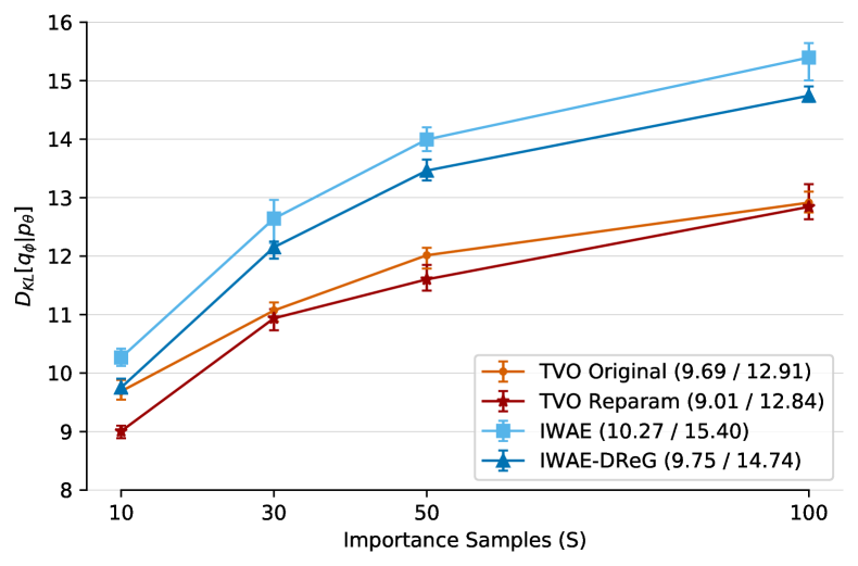
(b) Omniglot Test $D_{KL}[{q_{\phi}(\operatorname{\mathbf{z}}|\operatorname{\mathbf{x}})}||{p_{\theta}(\operatorname{\mathbf{z}}|\operatorname{\mathbf{x}})}]$

Figure 9: Model Learning and Inference by $S$ with $K=5$. Legend shows (min / max) values across $S$.

8 Experiments

We investigate the effect of our moment-spacing schedule and reparameterization gradients using a continuous latent variable model on the Omniglot dataset. We estimate test $\log p_{\theta}(\operatorname{\mathbf{x}})$ using the iwae bound (Burda et al., 2015) with 5k samples, and use $S=50$ samples for training unless noted. In all plots, we report averages over five random seeds, with error bars indicating min and max values. We describe our model architecture and experiment design in App. F, with runtimes and additional results on binary mnist in App. H.

Moment Spacing Dynamics

We seek understand the dynamics of our moment spacing schedule in Fig. 7, visualizing the choice of $\beta$ points across training epochs with $K=20$. Our intermediate distributions concentrate near $\beta=0$ at the beginning of training, since ${q_{\phi}(\operatorname{\mathbf{z}}|\operatorname{\mathbf{x}})}$ and ${p_{\theta}(\operatorname{\mathbf{z}}|\operatorname{\mathbf{x}})}$ are mismatched and the tvo integrand rises sharply away from ${q_{\phi}(\operatorname{\mathbf{z}}|\operatorname{\mathbf{x}})}$. This effect is particularly dramatic within the first five epochs.

While the curve is still fairly noisy within the first twenty epochs, it begins flatten as training progresses and ${q_{\phi}(\operatorname{\mathbf{z}}|\operatorname{\mathbf{x}})}$ learns to match ${p_{\theta}(\operatorname{\mathbf{z}}|\operatorname{\mathbf{x}})}$. This is reflected in the $\beta_{k}$ achieving a given proportion of the moments difference (eubo- elbo) moving to higher values. We found the moment-scheduling partitions to be relatively stable after 100 epochs.

Grid Search Comparison

Next, we fix $K=2$ with only $\beta_{1}$ chosen by the moment spacing schedule. We compare against grid search in Fig.  1 and Fig. 12 (App. H), and plot test $\log p_{\theta}(\operatorname{\mathbf{x}})$ as a function of $\beta_{1}\in[0,1]$ across 25 static values. We report the value of $\beta_{1}$ for our moments schedule at the final epoch, which indicates where $\eta_{\beta_{1}}$ is halfway between our estimated elbo and eubo.

We find that our adaptive scheduling matches the best performance from grid search, with the optimal intermediate distribution occurring at $\beta_{1}\approx 0.3$ on both datasets. With a single, properly chosen intermediate distribution, we find that the tvo can achieve notable improvements over the elbo at minimal additional cost.

Evaluating Scheduling Strategies

From a numerical integration perspective, the tvo bounds should become arbitrarily tight as $K\rightarrow\infty$. However, Masrani et al. (2019) observe that additional partitions can be detrimental for learning in practice. We thus investigate the performance of our moment spacing schedule with a varying number of partitions. We plot test log likelihood at $K=\{2,5,10,30,50\}$, and compare against three scheduling baselines: linear, log-uniform spacing, and the ‘coarse-grained’ schedule from Grosse et al. (2013) (see App. D.1). We begin the log-uniform spacing at $\beta_{1}=0.025$, a choice which results from grid search over $\beta_{1}$ for $K>2$ in Masrani et al. (2019).

We observe in Fig. 8(a) that the moment scheduler provides the best performance at high and low $K$, while the log-uniform schedule can perform best for particular $K$. As previously observed, all scheduling mechanisms still suffer degradation in performance at large $K$.

Reparameterized TVO Gradients

While our scheduling techniques do not address the detrimental effect of using many intermediate $\beta$, we now investigate the use of our reparameterization gradient estimator from Sec. 6. Repeating the previous experiment in Fig. 8(b), we find that reparameterization helps preserve competitive performance for high $K$ and improves overall model likelihoods. Our moments schedule is still particularly useful at low $K$, while the various scheduling methods converge to similar performance with many partition points. All scheduling techniques will be equivalent in the limit, as discussed in App. D.2.

Comparison with IWAE

Finally, we compare tvo with moments scheduling against the importance weighted autoencoder (iwae) (Burda et al., 2015) and doubly reparameterized iwaedreg (Tucker et al., 2018) for model learning and posterior inference. It is interesting to note that iwae corresponds to a direct estimate of $\psi(1)$, with the snis normalizer $\sum_{i=1}^{S}w_{i}^{1}$ in tvo (12) appearing inside the $\log$.

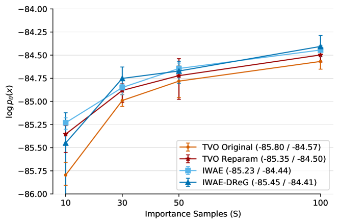
(a) MNIST Test $\log{p_{\theta}(\operatorname{\mathbf{x}})}$

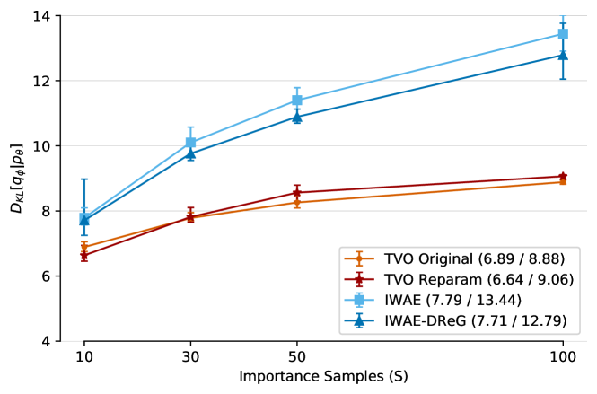
(b) MNIST Test $D_{KL}[{q_{\phi}(\operatorname{\mathbf{z}}|\operatorname{\mathbf{x}})}||{p_{\theta}(\operatorname{\mathbf{z}}|\operatorname{\mathbf{x}})}]$

Figure 13: Model Learning and Inference by $S$ (with $K=5$)

In Fig. 9, we observe that tvo with reparameterization gradients achieves model learning performance in between that of iwae and iwaedreg, with lower KL divergences across all values of $S$. We repeat this experiment for mnist in App. H Fig. 13, where tvo matches iwaedreg model learning with better inference. Although we tend to obtain lower $D_{KL}$ with lower model likelihood, we do not observe strong evidence of the signal-to-noise ratio issues of Rainforth et al. (2018) on either dataset. tvo with reparameterization thus appears to provide a favorable tradeoff between model learning and posterior inference.

9 Conclusion

In this work, we interpret the geometric mixture curve found in thermodynamic integration (ti), annealed importance sampling (ais), and the Thermodynamic Variational Objective (tvo), using the Bregman duality of exponential families. We leveraged this approach to characterize the gap in tvo lower and upper bounds as a sum of KL divergences along a given path, and presented an adaptive scheduling technique based on the mean parameterization of our exponential family. Finally, we derived a doubly-reparameterized gradient estimator for terms in the tvo integrand.

The use of self-normalized importance sampling (snis) to estimate expectations under $\pi_{\beta}$ may still be a key limitation of the tvo (see Masrani et al. (2019)), although we relied on the efficiency of snis for our moment-spacing schedule. Improved mcmc estimators that can be integrated with end-to-end learning of $q_{\phi}(\operatorname{\mathbf{z}}|\operatorname{\mathbf{x}})$ and $p_{\theta}(\operatorname{\mathbf{x}},\operatorname{\mathbf{z}})$ remain an intruiging direction for future work. In this study, we did not observe performance gains using equal spacing in either the KL or symmetrized KL divergence, but alternative schedules might also be motivated via physical interpretations (Andresen & Gordon, 1994; Salamon et al., 2002; Sivak & Crooks, 2012). We thus hope that our work can encourage further contributions in thermodynamic variational inference (tvi), a class of methods combining insights from vi, mcmc, and statistical physics.

Appendix A Conjugate Duality

The Bregman divergence associated with a convex function $f:\Omega\rightarrow\mathbb{R}$ can be written as (Banerjee et al., 2005):

$$D_{B_{f}}[p:q]=f(p)+f(q)-\langle p-q,\nabla f(q)\rangle$$

The family of Bregman divergences includes many familiar quantities, including the KL divergence corresponding to the negative entropy generator $f(p)=-\int p\log p\,d\omega$. Geometrically, the divergence can be viewed as the difference between $f(p)$ and its linear approximation around $q$. Since $f$ is convex, we know that a first order estimator will lie below the function, yielding $D_{f}[p:q]\geq 0$.

For our purposes, we can let $f\triangleq\psi(\beta)=\log Z_{\beta}$ over the domain of probability distributions indexed by natural parameters of an exponential family (e.g. (13)) :

$$D_{\psi}[\beta_{p}:\beta_{q}]=\psi(\beta_{p})-\psi(\beta_{q})-\langle\beta_{p}-\beta_{q},\nabla_{\beta}\psi(\beta_{q})\rangle$$ (34)

This is a common setting in the field of information geometry (Amari, 2016), which introduces dually flat manifold structures based on the natural parameters and the mean parameters.

A.1 KL Divergence as a Bregman Divergence

For an exponential family with partition function $\psi(\beta)$ and sufficient statistics $T(\omega)$ over a random variable $\omega$, the Bregman divergence $D_{\psi}$ corresponds to a KL divergence. Recalling that $\nabla_{\beta}\psi(\beta)=\eta_{\beta}=\mathbb{E}_{{\pi_{\beta}}}[T(\omega)]$ from Equation 16, we simplify the definition Equation 34 to obtain

$$D_{\psi}[\beta_{p}:\beta_{q}] =\psi(\beta_{p})-\psi(\beta_{q})-\beta_{p}\cdot\eta_{q}+\beta_{q}\cdot\eta_{q}$$

$$=\psi(\beta_{p})-\psi(\beta_{q})-\mathbb{E}_{q}[\beta_{p}\cdot T(\omega)]$$

$$\phantom{=\psi(\beta_{p})-\psi(\beta_{q})}+\mathbb{E}_{q}[\beta_{q}\cdot T(\omega)]$$

$$=\underbrace{\mathbb{E}_{q}\big{[}\beta_{q}\cdot T(\omega)-\psi(\beta_{q})\big{]}+\mathbb{E}_{q}[\pi_{0}(\omega)]}_{\log q(\omega)}$$

$$\phantom{=\mathbb{E}}-\underbrace{\mathbb{E}_{q}\big{[}\beta_{p}\cdot T(\omega)-\psi(\beta_{p})\big{]}-\mathbb{E}_{q}[\pi_{0}(\omega)]}_{\log p(\omega)}$$

$$=\mathbb{E}_{q}\log\frac{q(\omega)}{p(\omega)}$$

$$=D_{KL}[q(\omega)||p(\omega)]$$ (35)

where we have added and subtracted terms involving the base measure $\pi_{0}(\omega)$, and used the definition of our exponential family from (13). The Bregman divergence $D_{\psi}$ is thus equal to the KL divergence with arguments reversed.

A.2 Dual Divergence

We can leverage convex duality to derive an alternative divergence based on the conjugate function $\psi^{*}$.

$$\psi^{*}(\eta) =\sup\limits_{\beta}\,\eta\cdot\beta-\psi(\beta)\quad\implies\quad\eta=\nabla_{\beta}\,\psi(\beta)$$

$$=\eta\cdot\beta_{\eta}-\psi(\beta_{\eta})$$ (36)

The conjugate measures the maximum distance between the line $\eta\cdot\beta$ and the function $\psi(\beta)$, which occurs at the unique point $\beta_{\eta}$ where $\eta=\nabla_{\beta}\psi(\beta)$. This yields a bijective mapping between $\eta$ and $\beta$ for minimal exponential families (Wainwright & Jordan, 2008). Thus, a distribution $p$ may be indexed by either its natural parameters $\beta_{p}$ or mean parameters $\eta_{p}$.

Noting that $(\psi^{*})^{*}=\psi(\beta)=\sup_{\eta}\eta\cdot\beta-\psi^{*}(\eta)$ (Boyd & Vandenberghe, 2004), we can use a similar argument as above to write this correspondence as $\beta=\nabla_{\eta}\psi^{*}(\eta)$. We can then write the dual divergence $D_{\psi^{*}}$ as:

$$D_{\psi^{*}}[\eta_{p}:\eta_{q}] =\psi^{*}(\eta_{p})-\psi^{*}(\eta_{q})-\langle\eta_{p}-\eta_{q},\nabla_{\eta}\,\psi^{*}(\eta_{q})\rangle$$

$$=\psi^{*}(\eta_{p})-\underline{\psi^{*}(\eta_{q})}-\eta_{p}\cdot\beta_{q}+\underline{\eta_{q}\cdot\beta_{q}}$$

$$=\psi^{*}(\eta_{p})+\underline{\psi(\beta_{q})}-\eta_{p}\cdot\beta_{q}$$ (37)

where we have used  Equation 36 to simplify the underlined terms. Similarly,

$$D_{\psi}[\beta_{p}:\beta_{q}] =\psi(\beta_{p})-\psi(\beta_{q})-\langle\beta_{p}-\beta_{q},\nabla_{\beta}\psi(\beta_{q})\rangle$$

$$=\psi(\beta_{p})-\underline{\psi(\beta_{q})}-\beta_{p}\cdot\eta_{q}+\underline{\beta_{q}\cdot\eta_{q}}$$

$$=\psi(\beta_{p})+\underline{\psi^{*}(\eta_{q})}-\beta_{p}\cdot\eta_{q}$$ (38)

Comparing (37) and (38), we see that the divergences are equivalent with the arguments reversed, so that:

$$\vspace{-.25cm}D_{\psi}[\beta_{p}:\beta_{q}]=D_{\psi^{*}}[\eta_{q}:\eta_{p}]\vspace{-.25cm}$$ (39)

This indicates that the Bregman divergence $D_{\psi^{*}}$ should also be a KL divergence, but with the same order of arguments. We derive this fact directly in (44) , after investigating the form of the conjugate function $\psi^{*}$.

A.3 Conjugate $\psi^{*}$ as Negative Entropy

We first treat the case of an exponential family with no base measure $\pi_{0}(\omega)$, with derivations including a base measure in App. A.4. For a distribution $p$ in an exponential family, indexed by $\beta_{p}$ or $\eta_{p}$, we can write $\log p(\omega)=\beta_{p}\cdot T(\omega)-\psi(\beta)$. Then, (36) becomes:

$$\vspace{-.25cm}\psi^{*}(\eta_{p}) =\beta_{p}\cdot\eta_{p}-\psi(\beta_{p})$$ (40)

$$=\beta_{p}\cdot\mathbb{E}_{p}[T(\omega)]-\psi(\beta_{p})$$ (41)

$$=\mathbb{E}_{p}\log p(\omega)$$ (42)

$$=-H_{p}(\omega)\vspace{-.25cm}$$ (43)

since $\beta_{p}$ and $\psi(\beta_{p})$ are constant with respect to $\omega$. Utilizing $\psi^{*}(\eta_{p})=\mathbb{E}_{p}\log p(\omega)$ from above, the dual divergence with $q$ becomes:

$$\vspace*{-.25cm}D_{\psi^{*}}[\eta_{p}:\eta_{q}] =\psi^{*}(\eta_{p})-\psi^{*}(\eta_{q})-\langle\eta_{p}-\eta_{q},\nabla_{\eta}\,\psi^{*}(\eta_{q})\rangle$$

$$=\mathbb{E}_{p}\log p(\omega)-\underline{\psi^{*}(\eta_{q})}-\eta_{p}\cdot\beta_{q}+\underline{\eta_{q}\cdot\beta_{q}}$$

$$=\mathbb{E}_{p}\log p(\omega)-\eta_{p}\cdot\beta_{q}+\underline{\psi(\beta_{q})}$$

$$=\mathbb{E}_{p}\log p(\omega)-\mathbb{E}_{p}[T(\omega)\cdot\beta_{q}]+\psi(\beta_{q})$$

$$=\mathbb{E}_{p}\log p(\omega)-\mathbb{E}_{p}\log q(\omega)$$

$$=D_{KL}[p(\omega)||q(\omega)]\vspace*{-.25cm}$$ (44)

Thus, the conjugate function is the negative entropy and induces the KL divergence as its Bregman divergence (Wainwright & Jordan, 2008).

Note that, by ignoring the base distribution over $\omega$, we have instead assumed that $\pi_{0}(\omega):=u(\omega)$ is uniform over the domain. In the next section, we illustrate that the effect of adding a base distribution is to turn the conjugate function into a KL divergence, with the base $\pi_{0}(\omega)$ in the second argument. This is consistent with our derivation of negative entropy, since $D_{KL}[p_{\beta}(\omega)||u(\omega)]=-H_{p_{\beta}}(\Omega)+const$.

A.4 Conjugate $\psi^{*}$ as a KL Divergence

As noted above, the derivation of the conjugate $\psi^{*}(\eta)$ in (40)-(43) ignored the possibilty of a base distribution in our exponential family. We see that $\psi^{*}(\eta)$ takes the form of a KL divergence when considering a base measure $\pi_{0}(\omega)$.

$$\psi^{*}(\eta) =\sup\limits_{\beta}\beta\cdot\eta-\psi(\beta)$$ (45)

$$=\beta_{\eta}\cdot\eta-\psi(\beta_{\eta})$$

$$=\mathbb{E}_{\pi_{\beta_{\eta}}}[\beta_{\eta}\cdot T(\omega)]-\psi(\beta_{\eta})$$

$$=\mathbb{E}_{\pi_{\beta_{\eta}}}[\beta_{\eta}\cdot T(\omega)]-\psi(\beta_{\eta})\pm\mathbb{E}_{\pi_{\beta_{\eta}}}[\log\pi_{0}(\omega)]$$

$$=\mathbb{E}_{\pi_{\beta_{\eta}}}[\log\pi_{\beta_{\eta}(\omega)}-\log\pi_{0}(\omega)]$$

$$=D_{KL}[\pi_{\beta_{\eta}}(\omega)||\,\pi_{0}(\omega)]$$ (46)

Note that we have added and subtracted a factor of $\mathbb{E}_{\pi_{\beta_{\eta}}}\log\pi_{0}(\omega)$ in the fourth line, where our base measure $\pi_{0}(\omega)=q(\operatorname{\mathbf{z}}|\operatorname{\mathbf{x}})$ in the case of the tvo. Comparing with the derivations in (41)-(42), we need to include a term of $\mathbb{E}_{p}\pi_{0}(\omega)$ in moving to an expected log-probability $\mathbb{E}_{p}\log p(\omega)$, with the extra, subtracted base measure term transforming the negative entropy into a KL divergence.

In the tvo setting, this corresponds to

$$\psi^{*}(\eta)=D_{KL}[\pi_{\beta_{\eta}}(\operatorname{\mathbf{z}}|\operatorname{\mathbf{x}})||\,q(\operatorname{\mathbf{z}}|\operatorname{\mathbf{x}})]\,.$$ (47)

When including a base distribution, the induced Bregman divergence is still the KL divergence since, as in the derivation of Equation 35, both $\mathbb{E}_{p}\log p(\omega)$ and $\mathbb{E}_{p}\log q(\omega)$ will contain terms involving the base distribution $\mathbb{E}_{p}\log\pi_{0}(\omega)$.

Appendix B Renyi Divergence Variational Inference

In this section, we show that each intermediate partition function $\log Z_{\beta}$ corresponds to a scaled version of the Rényi VI objective $\mathcal{L}_{\alpha}$ (Li & Turner, 2016).

To begin, we recall the definition of Renyi’s $\alpha$ divergence.

$$D_{\alpha}[p||q]=\frac{1}{\alpha-1}\log\int q(\omega)^{1-\alpha}p(\omega)^{\alpha}d\omega$$

Note that this involves geometric mixtures similar to (14). Pulling out the factor of $\log p(\operatorname{\mathbf{x}})$ to consider normalized distributions over $\operatorname{\mathbf{z}}|\operatorname{\mathbf{x}}$, we obtain the objective of Li & Turner (2016). This is similar to the elbo, but instead subtracts a Renyi divergence of order $\alpha$.

$$\psi(\beta) =\log\int q(\operatorname{\mathbf{z}}|\operatorname{\mathbf{x}})^{1-\beta}p(\operatorname{\mathbf{x}},\operatorname{\mathbf{z}})^{\beta}d\operatorname{\mathbf{z}}$$

$$=\beta\log p(\operatorname{\mathbf{x}})-(1-\beta)D_{\beta}[{p_{\theta}(\operatorname{\mathbf{z}}|\operatorname{\mathbf{x}})}||{q_{\phi}(\operatorname{\mathbf{z}}|\operatorname{\mathbf{x}})}]$$

$$=\beta\log p(\operatorname{\mathbf{x}})-\beta\,D_{1-\beta}[{q_{\phi}(\operatorname{\mathbf{z}}|\operatorname{\mathbf{x}})}||{p_{\theta}(\operatorname{\mathbf{z}}|\operatorname{\mathbf{x}})}]$$

$$:=\beta\,\mathcal{L}_{1-\beta}$$

where we have used the skew symmetry property $D_{\alpha}[p||q]=\frac{\alpha}{1-\alpha}D_{1-\alpha}[q||p]$ for $0<\alpha<1$ (Van Erven & Harremos, 2014). Note that $\mathcal{L}_{0}=0$ and $\mathcal{L}_{1}=\log{p_{\theta}(\operatorname{\mathbf{x}})}$ as in Li & Turner (2016) and Sec. 3.

Appendix C TVO using Taylor Series Remainders

Recall that in Sec. 4, we have viewed the KL divergence $D_{\psi}[\beta:\beta^{\prime}]$ as the remainder in a first order Taylor approximation of $\psi(\beta)$ around $\beta^{\prime}$. The tvo objectives correspond to the linear term in this approximation, with the gap in $\operatorname{\textsc{tvo}}_{L}(\theta,\phi,\operatorname{\mathbf{x}})$ and $\operatorname{\textsc{tvo}}_{U}(\theta,\phi,\operatorname{\mathbf{x}})$ bounds amounting to a sum of KL divergences or Taylor remainders. Thus, the tvo may be viewed as a first order method.

Yet we may also ask, what happens when considering other approximation orders? We proceed to show that thermodynamic integration arises from a zero-order approximation, while the symmetrized KL divergence corresponds to a similar application of the fundamental theorem of calculus in the mean parameter space $\eta_{\beta}=\nabla_{\beta}\psi(\beta)$. In App. E, we briefly describe how ‘higher-order’ tvo objectives might be constructed, although these will no longer be guaranteed to provide upper or lower bounds on likelihood.

We will repeatedly utilize the integral form of the Taylor remainder theorem, which characterizes the error in a $k$-th order approximation of $\psi(x)$ around $a$, with $\beta\in[a,x]$. This identity can be derived using the fundamental theorem of calculus and repeated integration by parts (see, e.g. (Kountourogiannis & Loya, 2003) and references therein):

$$R_{k}(x)=\int_{a}^{x}\frac{\nabla_{\beta}^{(k+1)}\psi(\beta)}{k!}(x-\beta)^{k}d\beta$$ (48)

C.1 Thermodynamic Integration as $0^{th}$ Order Remainder

Consider a zero-order Taylor approximation of $\psi(1)$ around $a=0$, which simply uses $\psi(0)$ as an estimator. Applying the remainder theorem, we obtain the identity  Equation 6 underlying thermodynamic integration in the tvo:

$$\psi(1) =\psi(0)+R_{0}(1)$$ (49)

$$\psi(1)-\psi(0) =\int_{0}^{1}\nabla_{\beta}\psi(\beta)d\beta$$ (50)

$$\log{p_{\theta}(\operatorname{\mathbf{x}})} =\int_{0}^{1}\operatorname{\mathbb{E}}_{{\pi_{\beta}}}\bigg{[}{\log\frac{{p_{\theta}(\operatorname{\mathbf{x}},\operatorname{\mathbf{z}})}}{{q_{\phi}(\operatorname{\mathbf{z}}|\operatorname{\mathbf{x}})}}}\bigg{]}d\beta$$ (51)

where the last line follows as the definition of $\eta=\nabla_{\beta}\psi(\beta)=\nabla_{\beta}\log Z_{\beta}$ in  Equation 16.

Note that this integration is symmetric, in that approximating $\psi(0)$ using $\psi(1)$ leads to an equivalent expression after reversing the order of integration.

C.2 KL Divergence as $1^{st}$ Order Remainder

We can apply a similar approach to the first order Taylor approximations to reinterpret the TVO bound gaps in Equation 9 and Equation 10, although our remainder expressions will no longer be symmetric. We will thus distinguish between estimating $\psi(x)$ around $a<x$ and $a>x$ using $R_{1}^{\rightarrow}(x)$ and $R_{1}^{\leftarrow}(x)$, respectively, with the arrow indicating the direction of integration.

Estimating $\psi(\beta_{k})$ using a first order approximation around $a=\beta_{k-1}$ as in the tvo lower bound, the remainder exactly matches the definition of the Bregman divergence in Equation 19:

$$R_{1}^{\rightarrow}(\beta_{k}) =\psi(\beta_{k})-\big{(}\underbrace{\psi(\beta_{k-1})+(\beta_{k}-\beta_{k-1})\nabla_{\beta}\psi(\beta_{k-1})}_{\text{First-Order Taylor Approx}}\big{)}$$

$$=\int\limits_{\beta_{k-1}}^{\beta_{k}}\frac{\nabla_{\beta}^{2}\psi(\beta)}{1!}(\beta_{k}-\beta)^{1}d\beta$$ (52)

where (52) corresponds to the Taylor remainder from (48). Recall that this Bregman divergence $D_{\psi}[\beta_{k}:\beta_{k-1}]$ corresponds to a KL divergence $D_{KL}^{\,\rightarrow}[\pi_{\beta_{k-1}}||\pi_{\beta_{k}}]$ and contributes to the gap in $\operatorname{\textsc{tvo}}_{L}(\theta,\phi,\operatorname{\mathbf{x}})$.

Simplifying the Taylor remainder expression, with $\nabla^{2}_{\beta}\psi(\beta)=\operatorname{\mathrm{Var}}_{{\pi_{\beta}}}{\log\frac{{p_{\theta}(\operatorname{\mathbf{x}},\operatorname{\mathbf{z}})}}{{q_{\phi}(\operatorname{\mathbf{z}}|\operatorname{\mathbf{x}})}}}$, we obtain an integral representation of the KL divergence:

$$D_{KL}^{\,\rightarrow}[\pi_{\beta_{k-1}}||\pi_{\beta_{k}}]=\int\limits_{\beta_{k-1}}^{\beta_{k}}(\beta_{k}-\beta)\operatorname{\mathrm{Var}}_{{\pi_{\beta}}}{\log\frac{{p_{\theta}(\operatorname{\mathbf{x}},\operatorname{\mathbf{z}})}}{{q_{\phi}(\operatorname{\mathbf{z}}|\operatorname{\mathbf{x}})}}}d\beta$$ (53)

Following similar arguments in the reverse direction, we can obtain an integral form for the tvo upper bound gap $R_{1}^{\leftarrow}(\beta_{k-1})=D_{KL}[\pi_{\beta_{k}}||\pi_{\beta_{k-1}}]$ via the first-order approximation of $\psi(\beta_{k-1})$ around $a=\beta_{k}$.

$$R_{1}^{\leftarrow}(\beta_{k-1}) =\psi(\beta_{k-1})-\big{(}\psi(\beta_{k})+(\beta_{k-1}-\beta_{k})\nabla_{\beta}\psi(\beta_{k})\big{)}$$

$$=(\beta_{k}-\beta_{k-1})\nabla_{\beta}\psi(\beta_{k})-(\psi(\beta_{k})-\psi(\beta_{k-1}))$$

$$=\int\limits_{\beta_{k}}^{\beta_{k-1}}\frac{\nabla_{\beta}^{2}\psi(\beta)}{1!}(\beta_{k-1}-\beta)^{1}d\beta$$ (54)

Note that the tvo upper bound Equation 10 arises from the second line, with $R_{1}^{\leftarrow}(\beta_{k-1})\geq 0$ and $(\beta_{k}-\beta_{k-1})\nabla_{\beta}\psi(\beta_{k})$ corresponding to a right-Riemann approximation.

Switching the order of integration in (54), we can write the KL divergence as

$$D_{KL}^{\,\leftarrow}[\pi_{\beta_{k}}||\pi_{\beta_{k-1}}]=\int\limits_{\beta_{k-1}}^{\beta_{k}}(\beta-\beta_{k-1})\operatorname{\mathrm{Var}}_{{\pi_{\beta}}}{\log\frac{{p_{\theta}(\operatorname{\mathbf{x}},\operatorname{\mathbf{z}})}}{{q_{\phi}(\operatorname{\mathbf{z}}|\operatorname{\mathbf{x}})}}}d\beta$$ (55)

While these integral expressions for the KL divergence may not be immediately intuitive, our use of the Taylor remainder theorem unifies their derivation with that of thermodynamic integration. Alternative derivations may also be found in Dabak & Johnson (2002).

C.3 Symmetrized KL Divergence

Combining the expressions for the KL divergence in Eq. Equation 53 and Equation 55 immediately leads to a known result relating the symmetrized KL divergence to the integral of the Fisher information along the geometric path (Amari, 2016; Dabak & Johnson, 2002).

$${D_{KL}^{\,\,\leftrightarrow}} =(\beta_{k}-\beta_{k-1})\int\limits_{\beta_{k-1}}^{\beta_{k}}\operatorname{\mathrm{Var}}_{{\pi_{\beta}}}\bigg{[}{\log\frac{{p_{\theta}(\operatorname{\mathbf{x}},\operatorname{\mathbf{z}})}}{{q_{\phi}(\operatorname{\mathbf{z}}|\operatorname{\mathbf{x}})}}}d\beta\bigg{]}$$ (56)

where we have defined the symmetrized KL divergence as:

$${D_{KL}^{\,\,\leftrightarrow}}[\beta_{k-1};\beta_{k}]=D_{KL}^{\,\rightarrow}[\pi_{\beta_{k-1}}||\pi_{\beta_{k}}]+D_{KL}^{\,\leftarrow}[\pi_{\beta_{k}}||\pi_{\beta_{k-1}}]$$

Our goal in this section will be to show that (56) arises from similar ‘thermodynamic integration’ on the graph of the mean parameters $\eta_{\beta}$. Recall that we previously applied the fundamental theorem of calculus to $\psi(\beta)=\log Z_{\beta}$ to obtain the difference in log-partition functions

$$\psi(\beta_{k})-\psi(\beta_{k-1})=\int\limits_{\beta_{k-1}}^{\beta_{k}} \nabla_{\beta}\psi(\beta)d\beta$$

We can obtain a similar expression for the mean parameters $\eta_{\beta}=\nabla_{\beta}\psi(\beta)$ by integrating over the second derivative.

$$\eta_{k}-\eta_{k-1}=\int\limits_{\beta_{k-1}}^{\beta_{k}} \nabla_{\beta}^{2}\psi(\beta)d\beta$$ (57)

Recalling that $\nabla_{\beta}^{2}\psi(\beta)=\operatorname{\mathrm{Var}}_{{\pi_{\beta}}}{\log\frac{{p_{\theta}(\operatorname{\mathbf{x}},\operatorname{\mathbf{z}})}}{{q_{\phi}(\operatorname{\mathbf{z}}|\operatorname{\mathbf{x}})}}}$, we see that the integrands in  Equation 56 and Equation 57 are identical. Integrating with respect to $\beta$, we obtain the ‘area of a rectangle’ identity for the symmetrized KL divergence (as in (30)):

$${D_{KL}^{\,\,\leftrightarrow}}[\beta_{k-1};\beta_{k}] =\Delta_{\beta_{k}}\cdot\int\limits_{\beta_{k-1}}^{\beta_{k}}\operatorname{\mathrm{Var}}_{{\pi_{\beta}}}\bigg{[}{\log\frac{{p_{\theta}(\operatorname{\mathbf{x}},\operatorname{\mathbf{z}})}}{{q_{\phi}(\operatorname{\mathbf{z}}|\operatorname{\mathbf{x}})}}}d\beta\bigg{]}$$

$$=(\beta_{k}-\beta_{k-1})\int\limits_{\beta_{k-1}}^{\beta_{k}}\nabla^{2}_{\beta}\psi(\beta)d\beta$$

$$=(\beta_{k}-\beta_{k-1})\big{(}\nabla_{\beta}\psi(\beta)\,\big{|}_{\beta_{k-1}}^{\beta_{k}}\big{)}$$

$$=(\beta_{k}-\beta_{k-1})(\eta_{k}-\eta_{k-1})$$ (58)

This identity is best understood via Fig. 5 in Sec. 4.4.

To summarize, we have given several equivalent ways of understanding the symmetrized KL divergence.The ‘forward’ and ‘reverse’ KL divergences arise as gaps in the tvo left- and right-Riemann approximations (Figure 5), or first order Taylor remainders as in Equation 53 and Equation 55. Summing these quantities corresponds to the area of a rectangle Equation 58 on the graph of the tvo integrand $\eta_{\beta}$, or to the integral of a variance term via the Taylor remainder theorem  Equation 56 or fundamental theorem of calculus  Equation 57.

Note that the tvo integrand $\eta_{\beta}=\nabla_{\beta}\psi(\beta)=\mathbb{E}_{{\pi_{\beta}}}[{\log\frac{{p_{\theta}(\operatorname{\mathbf{x}},\operatorname{\mathbf{z}})}}{{q_{\phi}(\operatorname{\mathbf{z}}|\operatorname{\mathbf{x}})}}}]$ will be linear when its derivative, the variance of the log importance weights, is constant within $\beta\in[\beta_{k-1},\beta_{k}]$. The KL divergence is actually symmetric in this case, which we treat in more detail in the next section (App. D). More generally, the curvature of the integrand indicates which direction of the KL divergence has larger magnitude, and  Figure 5 reflects our empirical observations that $D_{KL}[\pi_{\beta_{k-1}}||\pi_{\beta_{k}}]>D_{KL}[\pi_{\beta_{k}}||\pi_{\beta_{k-1}}].$

Appendix D Asymptotic Linear Scheduling Analysis

Grosse et al. (2013) treat a quantity identical to $\operatorname{\textsc{tvo}}_{L}(\theta,\phi,\operatorname{\mathbf{x}})$ in the context of analysing the variance of ais estimators. Using the Central Limit Theorem, Neal (2001) show that the variance of an ais estimator is monotonically related to $\operatorname{\textsc{tvo}}_{L}(\theta,\phi,\operatorname{\mathbf{x}})$ under perfect transitions, or independent, exact samples from each intermediate $\beta$ (see Grosse et al. (2013) Eq. 3). However, note that ais estimates expectations over chains of $\operatorname{\textsc{mcmc}}$ samples rather than the simple reweighting used in the tvo.

In this section, we provide additional perspective on the analysis of Grosse et al. (2013), which considers the asymptotic behavior of the scaled gap in $\operatorname{\textsc{tvo}}_{L}(\theta,\phi,\operatorname{\mathbf{x}})$, $K\cdot D_{\underset{\rightarrow}{KL}}[\pi_{\beta_{k-1}}||\pi_{\beta_{k}}]$, as $K\rightarrow\infty$.

We begin by restating Theorem 1 of Grosse et al. (2013) for the case of the full tvo objective. We describe the resulting ‘coarse-grained’ linear binning schedule for choosing $\{\beta_{k}\}$ in D.1 and provide further analysis in D.2.

Theorem 1 (Grosse et al. (2013)).

Suppose $K+1$ distributions $\{\pi_{\beta_{k}}\}_{k=0}^{K}$ are linearly spaced along a path $\mathcal{P}$. Under the assumption of perfect transitions, if the Fisher information matrix $G(\beta)$ is smooth, then as $K\rightarrow\infty$:

$$K\sum\limits_{k=1}^{K}D_{KL}^{\,\rightarrow} [\pi_{\beta_{k-1}}||\pi_{\beta_{k}}]\rightarrow\frac{1}{2}\int\limits_{0}^{1}\dot{\beta}(t)\cdot G\big{(}\beta(t)\big{)}\cdot\dot{\beta}(t)dt$$ (59)

$$=\frac{1}{2}\big{(}D_{KL}^{\,\rightarrow}[\pi_{\beta_{0}}||\pi_{\beta_{K}}]+D_{KL}^{\,\leftarrow}[\pi_{\beta_{K}}||\pi_{\beta_{0}}]\big{)}$$

Here, we let $t\in[0,1]$ parameterize the path $\beta(t)=(1-t)\cdot\beta_{0}+t\cdot\beta_{K}$, and let $\dot{\beta}(t)$ denote the derivative of the parameter $\beta$ with respect to $t$. For linear mixing of the natural parameters as above, this is a constant: $\dot{\beta}(t)=\beta_{K}-\beta_{0}$. In the case of the full tvo integrand, $\dot{\beta}(t)=1$.

Proof.

See (Grosse et al., 2013) for a detailed proof, which proceeds by taking the Taylor expansion of $D_{KL}[\beta_{k}||\beta_{k}+\Delta_{\beta}]$ around each $\beta_{k}$ for small $\Delta_{\beta}$. In particular, $\Delta_{\beta}=\frac{1}{K}(\beta_{K}-\beta_{0})$ for linearly spaced $\beta_{k}=(1-\frac{k}{K})\cdot\beta_{0}+\frac{k}{K}\cdot\beta_{K}$. We assume w.l.o.g. $\beta_{K}-\beta_{0}=1$ and $\Delta_{\beta}=\frac{1}{K}$ as in Grosse et al. (2013) or tvo.

The zero- and first-order terms vanish, and the second-order term, with $\Delta_{\beta}^{2}=\frac{1}{K^{2}}$, can be written as (see e.g. Kullback (1997) p. 26):

$$K\sum\limits_{k=1}^{K}D_{KL}[\beta_{k}|| \beta_{k}+\Delta_{\beta}]=K\cdot\frac{1}{2K^{2}}\sum\limits_{k=1}^{K}\dot{\beta}_{k}\cdot G(\beta_{k})\cdot\dot{\beta}_{k}$$

$$\phantom{\beta_{k}+\Delta_{\beta}]=}+K\cdot\mathcal{O}(K^{-3})$$ (60)

$$\rightarrow\frac{1}{2}\,\int\limits_{0}^{1}\dot{\beta}(t)G\big{(}\beta(t)\big{)}\dot{\beta}(t)dt$$ (61)

where we have absorbed $\Delta_{\beta}=\frac{1}{K}$ into a continuous measure $dt$ as $K\rightarrow\infty$.

We now show that this expression corresponds to the symmetrized KL divergence, as in (Amari, 2016; Dabak & Johnson, 2002). While this was not stated in the theorem of Grosse et al. (2013), it has also been shown by e.g. Huszar (2017). Observe that $G(\beta)=\nabla_{\beta}\psi(\beta)=\text{Var}_{{\pi_{\beta}}}[T(\operatorname{\mathbf{x}},\operatorname{\mathbf{z}})]$ as in Equation 56 and Equation 58. Noting that the chain rule implies $\frac{d}{dt}G\big{(}\beta(t)\big{)}=\frac{d}{d\beta}G\big{(}\beta(t)\big{)}\frac{d\beta}{dt}$, we can pull one term of $\frac{d\beta}{dt}=\dot{\beta}(t)=(\beta_{K}-\beta_{0})$ outside the integral and perform integration by substitution. Ignoring the $1/2$ factor,

$$\frac{(\beta_{K}-\beta_{0})}{2}\, \int\limits_{0}^{1}G\big{(}\beta(t)\big{)}\frac{d\beta}{dt}dt=\frac{(\beta_{K}-\beta_{0})}{2}\int\limits_{\beta_{0}}^{\beta_{K}}\nabla_{\beta}^{2}\psi(\beta)d\beta$$

$$=\frac{1}{2}(\beta_{K}-\beta_{0})(\eta_{K}-\eta_{0})$$ (62)

$$=\frac{1}{2}\big{(}D_{KL}^{\,\rightarrow}[\pi_{\beta_{0}}||\pi_{\beta_{K}}]+D_{KL}^{\,\leftarrow}[\pi_{\beta_{K}}||\pi_{\beta_{0}}]\big{)}$$

∎

D.1 ‘Coarse-Grained’ Linear Schedule

Grosse et al. (2013) then use this asymptotic condition Equation 62 as $K\rightarrow\infty$ to inform the choice of a discrete partition $\mathcal{P}=\{\beta_{k}\}_{k=0}^{K}$.

More concretely, consider dividing the interval $[0,1]$ into $J$ equally-spaced knot points $\{\beta_{j}\}_{j=0}^{J}$. We then allocate a total budget of $K=\sum_{j=1}^{J}K_{j}$ intermediate distributions across sub-intervals $[\beta_{j-1},\beta_{j}]$, with uniform linear spacing of the $K_{j}$ partitions within each sub-interval.

Using Equation 62, Grosse et al. (2013) assign a cost $F_{j}=(\beta_{j}-\beta_{j-1})(\eta_{j}-\eta_{j-1})$ to each ‘coarse-grained’ interval $[\beta_{j-1},\beta_{j}]$. Minimizing $\sum_{j}F_{j}$ subject to $\sum_{j}K_{j}=K$, the allocation rule becomes:

$$K_{j}\propto\sqrt{(\beta_{j+1}-\beta_{j})(\eta_{j+1}-\eta_{j})}$$ (63)

We observe that performance when using this method can be sensitive to the number of knot points used, and we found $J=20$ to perform best in our experiments.

D.2 Additional Perspectives on Grosse et al. (2013)

Geometric Intuition for Theorem 1:

To further understand Theorem 1 of Grosse et al. (2013), observe that the tvo integrand will appear linear within any interval $[\beta_{k-1},\beta_{k}]$ as $K\rightarrow\infty$. For general endpoints $\beta_{0}$ and $\beta_{K}$, we let $\Delta_{\beta}=\beta_{k}-\beta_{k-1}=\frac{\beta_{K}-\beta_{0}}{K}$.

Having already visualized the symmetrized KL divergence as the area of a rectangle in Figure 5, we can see that each directed KL divergence, $D_{KL}^{\,\rightarrow}[\pi_{\beta_{k-1}}||\pi_{\beta_{k}}]$ and $D_{KL}^{\,\leftarrow}[\pi_{\beta_{k}}||\pi_{\beta_{k-1}}]$, will approach the area of triangle as the integrand becomes linear or $K\rightarrow\infty$, with area equal to $1/2\cdot\Delta_{\beta}\cdot\Delta_{\eta}$ . Then, the $D_{KL}$ scaled by $K$ becomes

$$K\sum\limits_{k=1}^{K}D_{KL}^{\,\rightarrow}[\pi_{\beta_{k-1}} ||\pi_{\beta_{k}}]\rightarrow K\sum\limits_{k=1}^{K}\frac{1}{2}\cdot\Delta_{\beta}\cdot\Delta_{\eta}$$ (64)

$$=K\sum\limits_{k=1}^{K}\frac{1}{2}(\frac{\beta_{K}-\beta_{0}}{K})\cdot(\eta_{k}-\eta_{k-1})$$

$$=\frac{1}{2}(\beta_{K}-\beta_{0})\cdot(\eta_{K}-\eta_{0})\,.$$

where, in the last line, we cancel factors of $K$ and note the cancellation of intermediate $\eta_{k}$ in the telescoping sum.

Thermodynamic Interpretation:

This limiting behavior is also discussed in thermodynamics, where the LHS of Equation 64 and Equation 59 corresponds to the rate of entropy production in transitioning a system from $\pi_{\beta_{0}}$ to $\pi_{\beta_{1}}$ along a path defined by $\{\beta_{k}\}$. The condition that $K\rightarrow\infty$ refers to the quasi-static limit, in which the system is allowed to remain at equilibrium throughout the process (e.g. Crooks (2007)).

Exponential and Mixture Geodesics:

As in the statement of Theorem 1, we can more generally consider connecting two distributions, indexed by natural parameters $\beta_{0}$ and $\beta_{1}$, using a parameter $t\in[0,1]$. The curve $\beta_{t}=(1-t)\cdot\beta_{0}+t\cdot\beta_{1}$ then corresponds to our path exponential family Equation 13, and is also referred to as the $e$-geodesic in information geometry Amari (2016).

Similarly, the moment-averaged path of Grosse et al. (2013), which also underlies our scheduling strategy in Sec. 5, can be viewed as a linear mixture in the mean parameter space. The $m$-geodesic then refers to the curve $\eta_{t}=(1-t)\cdot\eta_{0}+t\cdot\eta_{1}$ (Amari, 2016). Note that these mixtures reference different distribution for the same parameter $t$, so that $\eta_{\beta_{t}}\neq\eta_{t}$.

Grosse et al. (2013) proceed to show that the expression for the symmetric KL divergence (59) corresponds to the integral of the Fisher information along either the geometric or mixture paths (Theorem 2 of Grosse et al. (2013), Theorem 3.2 of Amari (2016)). The union of the intermediate distributions integrated by these two paths coincide in our one-dimensional exponential family, although this intuition does not appear to translate to higher dimensions.

Appendix E Higher Order tvo

While the convexity of the log-partition function yields the family of Bregman divergences from the remainder in the first order Taylor approximation, we might also consider higher order terms to obtain tighter bounds on likelihood or analyse properties of the TVO integrand $\nabla_{\beta}\psi(\beta)$. We give an example derivation for a second-order tvo objectives, although these are no longer guaranteed to be upper or lower bounds on likelihood.

Left-to-Right Expansion

We first consider expanding the approximations in the tvo left-Riemann sum to second order. We denote the resulting objective $\mathcal{L}_{\rightarrow}^{(2)}$, since we move ‘left-to-right’ in estimating $\psi(\beta_{k})$ around $\beta_{k-1}$. We begin by writing the second-order Taylor approximation:

$$\psi(\beta_{k}) \approx\psi(\beta_{k-1})+(\beta_{k}-\beta_{k-1})\,\nabla_{\beta}\psi(\beta_{k-1})$$

$$\phantom{\approx}+\frac{1}{2}(\beta_{k}-\beta_{k-1})^{2}\,\nabla_{\beta}^{2}\psi(\beta_{k-1})$$ (65)

While $\operatorname{\textsc{tvo}}_{L}(\theta,\phi,\operatorname{\mathbf{x}})$ consists of the first-order term alone, we can also consider adding the non-negative, second-order term to form the objective $\mathcal{L}_{\rightarrow}^{(2)}$. Using successive Taylor approximations of $\psi(\beta_{k})$, we obtain similar telescoping cancellations to obtain

$$\log p(\operatorname{\mathbf{x}})-\mathcal{L}_{\rightarrow}^{(2)} =\log p(\operatorname{\mathbf{x}})-\sum\limits_{k=1}^{K}(\beta_{k}-\beta_{k-1})\cdot\eta_{\beta_{k-1}}$$

$$-\sum\limits_{k=1}^{K}\frac{1}{2}(\beta_{k}-\beta_{k-1})^{2}\,\text{Var}_{\pi_{\beta_{k-1}}}\log\frac{p(\operatorname{\mathbf{x}},\operatorname{\mathbf{z}})}{q(\operatorname{\mathbf{z}}|\operatorname{\mathbf{x}})}$$ (66)

where $\eta_{\beta_{k-1}}=\mathbb{E}_{\pi_{\beta_{k-1}}}\log\frac{p(\operatorname{\mathbf{x}},\operatorname{\mathbf{z}})}{q(\operatorname{\mathbf{z}}|\operatorname{\mathbf{x}})}$.

We previously obtained a lower bound on log-likelihood via this construction, with $\log p(\operatorname{\mathbf{x}})-\operatorname{\textsc{tvo}}_{L}(\theta,\phi,\operatorname{\mathbf{x}})\geq 0$. However, $\mathcal{L}_{\rightarrow}^{(2)}$ will only provide a lower bound if $\nabla_{\beta}\psi(\beta)$ is concave, i.e. $\nabla^{3}_{\beta}\psi(\beta)\leq 0.$ To see this, we write the Taylor remainder Equation 48 as

$$R_{2}^{\rightarrow}(\beta_{k}) =\int\limits_{\beta_{k-1}}^{\beta_{k}}\frac{1}{6}(\beta_{k}-\beta_{t})^{3}\,\nabla_{\beta}^{3}\psi(\beta_{t})d\beta_{t}$$ (67)

with the third derivative equal to

$$\nabla_{\beta}^{3}\psi(\beta) =\mathbb{E}_{\pi_{\beta}}[T(\operatorname{\mathbf{x}},\operatorname{\mathbf{z}})^{3}]-3\,[\mathbb{E}_{\pi_{\beta}}T(\operatorname{\mathbf{x}},\operatorname{\mathbf{z}})]\cdot\mathbb{E}_{\pi_{\beta}}[T(\operatorname{\mathbf{x}},\operatorname{\mathbf{z}})^{2}]$$

$$\phantom{=}+2[\mathbb{E}_{\pi_{\beta}}T(\operatorname{\mathbf{x}},\operatorname{\mathbf{z}})]^{3}$$

$$=\mathbb{E}_{\pi_{\beta}}[T(\operatorname{\mathbf{x}},\operatorname{\mathbf{z}})^{3}]-[\mathbb{E}_{\pi_{\beta}}T(\operatorname{\mathbf{x}},\operatorname{\mathbf{z}})]^{3}$$

$$\phantom{=}-3[\mathbb{E}_{\pi_{\beta}}T(\operatorname{\mathbf{x}},\operatorname{\mathbf{z}})]\cdot[\text{Var}_{\pi_{\beta}}T(\operatorname{\mathbf{x}},\operatorname{\mathbf{z}})]$$

In addition to indicating that $\mathcal{L}_{\rightarrow}^{(2)}$ is a lower bound on $\log{p_{\theta}(\operatorname{\mathbf{x}})}$, testing the concavity of $\nabla_{\beta}\psi(\beta)$ using $\nabla^{3}_{\beta}\psi(\beta)\leq 0$ can also indicate whether a trapezoid approximation to the tvo integral provides a valid lower bound.

We can give an identical construction for the reverse direction $\mathcal{L}_{\leftarrow}^{(2)}$ or higher order approximations. We leave a full exploration of these objectives for future work.

Appendix F Experimental Setup

Code for all experiments can be found at https://github.com/vmasrani/tvo_all_in.

Model

Following (Burda et al., 2015), we use a variational autoencoder (Kingma & Welling, 2013) with a 50-dimensional stochastic layer, $\operatorname{\mathbf{z}}\in\operatorname{\mathcal{R}}^{50}$

$$p_{\theta}(\operatorname{\mathbf{x}},\operatorname{\mathbf{z}}) =p_{\theta}(\operatorname{\mathbf{x}}|\operatorname{\mathbf{z}})p(\operatorname{\mathbf{z}})$$

$$p(\operatorname{\mathbf{z}}) =\operatorname{\mathcal{N}}(\operatorname{\mathbf{z}}|0,\operatorname{\mathbf{I}})$$

$$p_{\theta}(\operatorname{\mathbf{x}}|\operatorname{\mathbf{z}}) =\operatorname{Bern}(\operatorname{\mathbf{x}}|\text{decoder}_{\theta}(\operatorname{\mathbf{z}}))$$

$$q_{\phi}(\operatorname{\mathbf{z}}|\operatorname{\mathbf{x}}) =\operatorname{\mathcal{N}}(\operatorname{\mathbf{z}};\boldsymbol{\mu}_{\phi}(\operatorname{\mathbf{x}}),\boldsymbol{\sigma}_{\phi}(\operatorname{\mathbf{x}}))$$

where the encoder and decoder are each two-layer MLPs with tanh activations and 200 hidden dimensions. The output of the encoder is duplicated and passed through an additional linear layer to parameterize the mean and log-standard deviation of a conditionally independent Normal distribution. The output of the decoder is a sigmoid which parameterizes the probabilities of the independent Bernoulli distribution. $\theta$ and $\phi$ refer to the weights of the decoder and encoder, respectively.

Dataset

We use Omniglot (Lake et al., 2013), a dataset of 1623 handwritten characters across 50 alphabets. Each datapoint is binarized $28\times 28$ image, i.e $\operatorname{\mathbf{x}}\in\{0,1\}^{784}$, where we follow the common procedure in the literature of sampling each binary-valued observation with expectation equal to the real pixel value (Salakhutdinov & Murray, 2008; Burda et al., 2015). We split the dataset into 24,345 training and 8,070 test examples.

Training Procedure

All models are written in PyTorch and trained on GPUs. For each scheduler, we train for 5000 epochs using the Adam optimizer (Kingma & Ba, 2017) with a learning rate of $10^{-3}$, and minibatch size of 1000. All weights are initialized with PyTorch’s default initializer.

Appendix G Implementation Details

While the Legendre transform, mapping between a target value of expected sufficient statistics $\eta=\mathbb{E}_{{\pi_{\beta}}}[T(\omega)]$ and the appropriate natural parameters $\beta$, can be a difficult problem in general, we describe how to efficiently implement our ‘moments-spacing’ schedule in the context of tvo.

Recall from Sec. 5 that we are interested in finding a discrete partition $\mathcal{P}_{\beta}=\{\beta_{k}\}_{k=0}^{K}$ such that:

$$\beta_{k}=\eta^{-1}_{\beta}\left(\frac{k}{K}\cdot\lx@glossaries@gls@link{acronym}{ELBO}{\leavevmode\textsc{elbo}}+(1-\frac{k}{K})\cdot\lx@glossaries@gls@link{acronym}{EUBO}{\leavevmode\textsc{eubo}}\right)$$ (68)

In other words, we seek to find the $\beta_{k}$ such that $\mathbb{E}_{\pi_{\beta_{k}}}[{\log\frac{{p_{\theta}(\operatorname{\mathbf{x}},\operatorname{\mathbf{z}})}}{{q_{\phi}(\operatorname{\mathbf{z}}|\operatorname{\mathbf{x}})}}}]\approx\eta_{k}$, where $\eta_{k}$ are equally spaced between the elbo and eubo (see Figure 6).

Figure 10: Pseudo-code Implementation of Moments Scheduling for tvo

⬇

1# Calculate expected sufficient statistics eta at a given beta (Eq. 12)

2def calc_eta(log_iw, beta):

3 # 1) Exponentiate/normalize over importance sample dimension

4 snis = torch.exp(log_iw*beta -

5 torch.logsumexp(log_iw*beta,

6 dim = 1, keepdim=True))

7 # 2) Take mean over data examples

8 return torch.mean(snis*log_iw, dim =0)

9

10def binary_search(target, log_iw, start=0, stop=1, threshold = 0.1):

11

12 beta_guess = .5*(stop-start)

13 eta_guess = calc_eta(log_iw,beta_guess)

14 if eta_guess > target + threshold:

15 return binary_search(

16 target,

17 log_iw,

18 start=beta_guess,

19 stop=stop)

20 elif eta_guess < target - threshold:

21 return binary_search(

22 target,

23 log_iw,

24 start=start,

25 stop=beta_guess)

26 else:

27 return beta_guess

⬇

1

2def moments_spacing_schedule(log_iw, K, search=’binary’):

3 # 1) Calculate target values for uniform moments spacing

4 elbo = calc_eta(log_iw, 0)

5 eubo = calc_eta(log_iw, 1)

6 targets = [(1-t)*elbo+t*eubo

7 for t in np.linspace(0,1,K+1)]

8

9 # 2) Find beta corresponding to each target (including beta=0,1)

10 beta_schedule = [0]

11

12 for _k in range(1, K):

13 target_eta = targets[_k]

14

15 beta_k = binary_search(

16 target_eta,

17 log_iw,

18 start = 0,

19 stop = 1)

20

21 beta_schedule.append(beta_k)

22

23 beta_schedule.append(1)

24 # 3) Return beta_schedule: used for Riemann approximation points in TVO objective

25 return beta_schedule

More concretely, we provide pseudo-code implementing our moments spacing schedule below. Given a set of $S$ log-importance weights per sample, and a number of intermediate distributions $K$:

Appendix H Additional Results

In this section, we report wall-clock runtimes and run similar experiments as in Sec. 8 to evaluate our moments spacing schedule and reparameterized gradients on the binarized MNIST dataset (Salakhutdinov & Murray, 2008).

Wall-Clock Times

We report wall clock runtimes for various scheduling methods with $S=50$ and $K=5$ in Fig. 11. While tvo methods require slight overhead compared with iwae, our adaptive moments scheduler does not require significantly more computation than the log-uniform baseline.

Grid Search Comparison

We evaluate our moments schedule with $K=2$ against grid search over the choice of a single intermediate $\beta_{1}$ in Fig. 12. The setup is similar to that of Fig. 1 on Omniglot (see Sec. 8), but here we use reparameterization gradients instead of the original tvo. Here, we train for 1000 epochs using an Adam optimizer with learning rate $10^{-3}$ and batch size 100.

We again find that our moments spacing schedule arrives at an optimal choice of $\beta_{1}$, and can even outperform the best static value due to its ability to adaptively update at each epoch. It is interesting to note that the final choice of $\beta_{1}$, which reflects the shape of the tvo integrand, is nearly identical at $\beta_{1}\approx 0.30$ across both mnist and Omniglot.

Comparison with IWAE

We compare tvo using our moments scheduling against the iwae and iwae dreg as in Fig. 9 of the main text. We find that our tvo reparameterized gradient estimator achieves nearly identical model learning performance as iwae and iwae dreg, with notably improved posterior inference for all values of $S$.

Evaluating Scheduling Strategies

In the Fig. 14-17 below, we reproduce the setting of Fig. 8 to evaluate our scheduling strategies by $K$, for tvo with both $\operatorname{\textsc{reinforce}}$ and reparameterized gradient estimators, on Omniglot and mnist. We also report posterior inference results as measured by test $D_{KL}[{q_{\phi}(\operatorname{\mathbf{z}}|\operatorname{\mathbf{x}})}||{p_{\theta}(\operatorname{\mathbf{z}}|\operatorname{\mathbf{x}})}]$. In general, we find comparable performance between our moments schedule and the log-uniform baseline, although our approach performs best with $K=2$ and does not require grid search. Further, on mnist with batch size 1000 and low $K$, log-uniform, linear, and coarse-grained schedules suffer from poor performance due to instability in training, which is avoided by our moments schedule. Training can be stabilized by using smaller batch sizes as in Fig. 12.

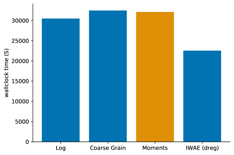
Figure 11: Omniglot Runtimes ($S=50$, $K=5$, 5k epochs)

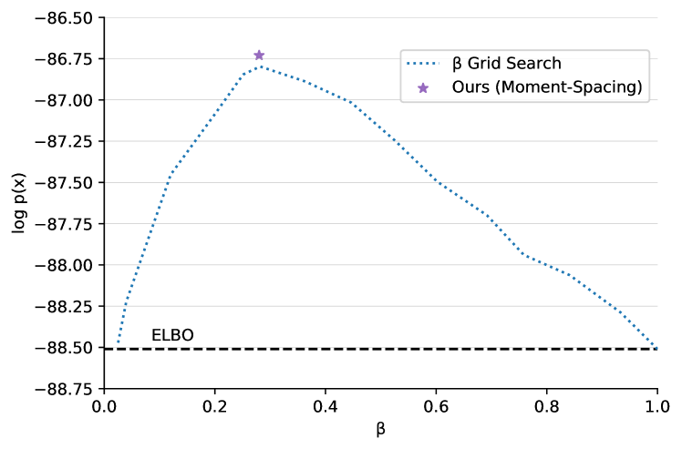
Figure 12: MNIST $K=2$, with reparameterization gradients.

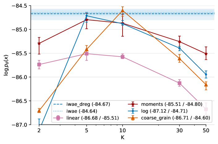
(a) MNIST Test $\log{p_{\theta}(\operatorname{\mathbf{x}})}$

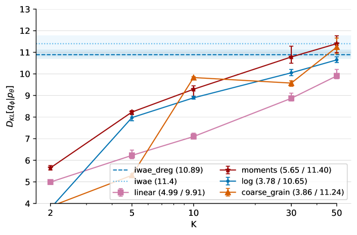
(b) MNIST Test $D_{KL}[{q_{\phi}(\operatorname{\mathbf{z}}|\operatorname{\mathbf{x}})}||{p_{\theta}(\operatorname{\mathbf{z}}|\operatorname{\mathbf{x}})}]$

Figure 14: tvo with $\operatorname{\textsc{reinforce}}$ Gradients: Model Learning and Inference by $K$ (with $S=50$)

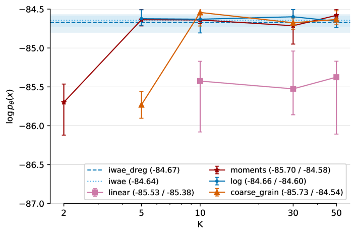
(a) MNIST Test $\log{p_{\theta}(\operatorname{\mathbf{x}})}$

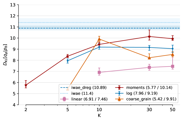
(b) MNIST Test $D_{KL}[{q_{\phi}(\operatorname{\mathbf{z}}|\operatorname{\mathbf{x}})}||{p_{\theta}(\operatorname{\mathbf{z}}|\operatorname{\mathbf{x}})}]$

Figure 15: tvo with Reparameterized Gradients: Model Learning and Inference by $K$ (with $S=50$)

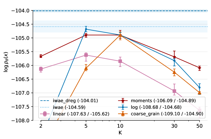
(a) Omniglot Test $\log{p_{\theta}(\operatorname{\mathbf{x}})}$

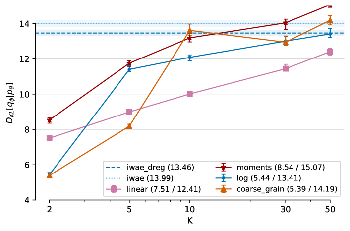
(b) Omniglot Test $D_{KL}[{q_{\phi}(\operatorname{\mathbf{z}}|\operatorname{\mathbf{x}})}||{p_{\theta}(\operatorname{\mathbf{z}}|\operatorname{\mathbf{x}})}]$

Figure 16: tvo with $\operatorname{\textsc{reinforce}}$ Gradients: Model Learning and Inference by $K$ (with $S=50$)

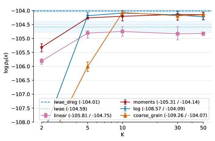
(a) Omniglot Test $\log{p_{\theta}(\operatorname{\mathbf{x}})}$

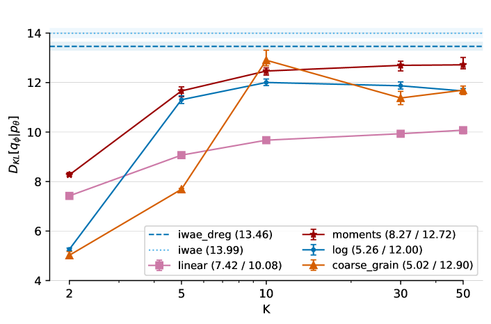
(b) Omniglot Test $D_{KL}[{q_{\phi}(\operatorname{\mathbf{z}}|\operatorname{\mathbf{x}})}||{p_{\theta}(\operatorname{\mathbf{z}}|\operatorname{\mathbf{x}})}]$

Figure 17: tvo with Reparameterized Gradients: Model Learning and Inference by $K$ (with $S=50$)

Appendix I Reparameterization Gradients for the TVO Integrand

Recall that the tvo objective involves terms of the form

$$\mathbb{E}_{{\pi_{\beta}}}\left[f(\operatorname{\mathbf{z}})\right]\quad\text{where}\quad{\pi_{\beta}}(\operatorname{\mathbf{z}}|\operatorname{\mathbf{x}})=\frac{{q_{\phi}(\operatorname{\mathbf{z}}|\operatorname{\mathbf{x}})}^{1-\beta}{p_{\theta}(\operatorname{\mathbf{x}},\operatorname{\mathbf{z}})}^{\beta}}{Z_{\beta}}\quad\text{and}\quad f(\operatorname{\mathbf{z}})=\log\frac{{p_{\theta}(\operatorname{\mathbf{x}},\operatorname{\mathbf{z}})}}{{q_{\phi}(\operatorname{\mathbf{z}}|\operatorname{\mathbf{x}})}}$$ (69)

While Masrani et al. (2019) derive a $\operatorname{\textsc{reinforce}}$-style gradient estimator for the tvo, we seek to apply the reparameterization trick when possible, and thus differentiate with respect to only the inference network parameters $\phi$. Note that, for $\operatorname{\mathbf{z}}_{i}\sim{q_{\phi}(\operatorname{\mathbf{z}}|\operatorname{\mathbf{x}})}$ reparameterizable with $\operatorname{\mathbf{z}}=z(\epsilon,\phi)$ and $\epsilon_{i}\sim p(\epsilon)$, any expectation under $\pi_{\beta}$ can be written as

$${\mathbb{E}_{\pi_{\beta}}}\left[f(\operatorname{\mathbf{z}})\right]=\frac{1}{Z_{\beta}}\mathbb{E}_{{q_{\phi}(\operatorname{\mathbf{z}}|\operatorname{\mathbf{x}})}}\left[w^{\beta}f(\operatorname{\mathbf{z}})\right]=\frac{1}{Z_{\beta}}\mathbb{E}_{\epsilon}\left[w^{\beta}f(\operatorname{\mathbf{z}})\right]\quad\text{where}\quad w=\frac{{p_{\theta}(\operatorname{\mathbf{x}},\operatorname{\mathbf{z}})}}{{q_{\phi}(\operatorname{\mathbf{z}}|\operatorname{\mathbf{x}})}}$$ (70)

In differentiating Equation 70, we will frequently encounter terms of the form $\mathbb{E}_{{\pi_{\beta}}}\left[f(\operatorname{\mathbf{z}})\frac{d}{d\phi}\log\frac{{p_{\theta}(\operatorname{\mathbf{x}},\operatorname{\mathbf{z}})}}{{q_{\phi}(\operatorname{\mathbf{z}}|\operatorname{\mathbf{x}})}}\right]$ for generic $f(\operatorname{\mathbf{z}})$. Noting that the total derivative contains score function partial derivatives, we apply the reparameterization trick to these terms in an approach similar to the ‘doubly-reparameterized’ estimator of Tucker et al. (2018). The following lemma summarizes these calculations, rewritten using expectations under $\pi_{\beta}$ as in Equation 70.

Lemma 1.

Let $f(\operatorname{\mathbf{z}}):\mathbb{R}^{M}\mapsto\mathbb{R}$, ${\pi_{\beta}}(\operatorname{\mathbf{z}}|\operatorname{\mathbf{x}})$, and $w=\frac{{p_{\theta}(\operatorname{\mathbf{x}},\operatorname{\mathbf{z}})}}{{q_{\phi}(\operatorname{\mathbf{z}}|\operatorname{\mathbf{x}})}}$ all depend on $\phi$. When $\operatorname{\mathbf{z}}\sim{q_{\phi}(\operatorname{\mathbf{z}}|\operatorname{\mathbf{x}})}$ is reparameterizable via $\operatorname{\mathbf{z}}=z(\epsilon,\phi),\,\epsilon\sim p(\epsilon)$, the following identity holds for expectations under ${\pi_{\beta}}$

$$\mathbb{E}_{{\pi_{\beta}}}\left[f(\operatorname{\mathbf{z}})\frac{d}{d\phi}\log w\right]=\mathbb{E}_{\pi_{\beta}}\left[{\frac{\partial\operatorname{\mathbf{z}}}{\partial\phi}}\left((1-\beta)f(\operatorname{\mathbf{z}})\frac{\partial\log w}{\partial\operatorname{\mathbf{z}}}-{\frac{\partial f(\operatorname{\mathbf{z}})}{\partial\operatorname{\mathbf{z}}}}\right)\right].$$ (71)

Proof.

See § I.3. ∎

Corollary 1.1.

For the choice of $f(\operatorname{\mathbf{z}})=1$ we obtain

$$\mathbb{E}_{{\pi_{\beta}}}\left[\frac{d}{d\phi}\log w\right]=(1-\beta)\,\mathbb{E}_{\pi_{\beta}}\left[{\frac{\partial\operatorname{\mathbf{z}}}{\partial\phi}}\frac{\partial\log w}{\partial\operatorname{\mathbf{z}}}\right]$$ (72)

The following lemma will allow us to apply reparameterization within the normalization constant.

Lemma 2.

Let the same conditions hold as in Lemma 1, with $Z_{\beta}=\int{q_{\phi}(\operatorname{\mathbf{z}}|\operatorname{\mathbf{x}})}^{1-\beta}p_{\theta}(\operatorname{\mathbf{x}},\operatorname{\mathbf{z}})^{\beta}\operatorname{d\mathbf{z}}$. Then

$$\frac{d}{d\phi}Z_{\beta}=\beta(1-\beta)\,\mathbb{E}_{\epsilon}\left[w^{\beta}{\frac{\partial\operatorname{\mathbf{z}}}{\partial\phi}}\frac{\partial\log w}{\partial\operatorname{\mathbf{z}}}\right].$$ (73)

Proof.

See § I.4. ∎

We now proceed to differentiate the TVO integrand given by Equation 69.

I.1 Reparameterized tvo Gradient Estimator

For generic $f(\operatorname{\mathbf{z}}):\mathbb{R}^{M}\mapsto\mathbb{R}$ and reparameterizable $\operatorname{\mathbf{z}}\sim{q_{\phi}(\operatorname{\mathbf{z}}|\operatorname{\mathbf{x}})}$ as above, the gradient with respect to $\phi$ can be written as

$$\frac{d}{d\phi}\mathbb{E}_{{\pi_{\beta}}}\left[f(\operatorname{\mathbf{z}})\right] =\mathbb{E}_{{\pi_{\beta}}}\left[\left(\frac{d}{d\phi}f(\operatorname{\mathbf{z}})\right)-\beta\left(\frac{\partial\operatorname{\mathbf{z}}}{\partial\phi}\frac{\partial f(\operatorname{\mathbf{z}})}{\partial\operatorname{\mathbf{z}}}\right)\right]+\beta(1-\beta)\text{Cov}_{\pi_{\beta}}\left[f(\operatorname{\mathbf{z}}),\frac{\partial\operatorname{\mathbf{z}}}{\partial\phi}\frac{\partial\log w}{\partial\operatorname{\mathbf{z}}}\right].$$ (74)

The gradient of the tvo integrand is of particular interest. For $f(\operatorname{\mathbf{z}})=\log w$ with $w=\frac{{p_{\theta}(\operatorname{\mathbf{x}},\operatorname{\mathbf{z}})}}{{q_{\phi}(\operatorname{\mathbf{z}}|\operatorname{\mathbf{x}})}}$, Equation 74 simplifies to

$$\frac{d}{d\phi}\mathbb{E}_{{\pi_{\beta}}}\left[\log w\right] =(1-2\beta)\mathbb{E}_{{\pi_{\beta}}}\left[\frac{\partial\operatorname{\mathbf{z}}}{\partial\phi}\frac{\partial\log w}{\partial\operatorname{\mathbf{z}}}\right]+\beta(1-\beta)\text{Cov}_{\pi_{\beta}}\left[\log w,\frac{\partial\operatorname{\mathbf{z}}}{\partial\phi}\frac{\partial\log w}{\partial\operatorname{\mathbf{z}}}\right].$$ (75)

Proof.

We track changes between lines in blue, and begin by applying the product rule.

$$\frac{d}{d\phi}\mathbb{E}_{{\pi_{\beta}}}\left[f(\operatorname{\mathbf{z}})\right] =\frac{d}{d\phi}\left(Z_{\beta}^{-1}\mathbb{E}_{\epsilon}\left[w^{\beta}\,f(\operatorname{\mathbf{z}})\right]\right)$$ (76)

$$={\color[rgb]{0,0,1}\left(\frac{d}{d\phi}Z_{\beta}^{-1}\right)}\mathbb{E}_{\epsilon}\left[w^{\beta}\,f(\operatorname{\mathbf{z}})\right]+Z_{\beta}^{-1}\mathbb{E}_{\epsilon}\left[f(\operatorname{\mathbf{z}}){\color[rgb]{0,0,1}\left(\frac{d}{d\phi}w^{\beta}\right)}\right]+Z_{\beta}^{-1}\mathbb{E}_{\epsilon}\left[w^{\beta}{\color[rgb]{0,0,1}\left(\frac{d}{d\phi}f(\operatorname{\mathbf{z}})\right)}\right]$$ (77)

$$={\color[rgb]{0,0,1}\left(\frac{d}{d\phi}Z_{\beta}\right)\left(\frac{-1}{Z_{\beta}^{2}}\right)}\mathbb{E}_{\epsilon}\left[w^{\beta}\,f(\operatorname{\mathbf{z}})\right]+Z_{\beta}^{-1}\mathbb{E}_{\epsilon}\left[{\color[rgb]{0,0,1}\beta w^{\beta}\,f(\operatorname{\mathbf{z}})\left(\frac{d}{d\phi}\log w\right)}\right]+Z_{\beta}^{-1}\mathbb{E}_{\epsilon}\left[w^{\beta}\left(\frac{d}{d\phi}f(\operatorname{\mathbf{z}})\right)\right]$$ (78)

$$=\underbrace{\left(\frac{d}{d\phi}Z_{\beta}\right){\color[rgb]{0,0,1}\left(\frac{-1}{Z_{\beta}}\right)}\mathbb{E}_{{\color[rgb]{0,0,1}{\pi_{\beta}}}}\left[f(\operatorname{\mathbf{z}})\right]}_{\raisebox{0.5pt}{\raisebox{-.9pt} {1}⃝}}+\underbrace{{\color[rgb]{0,0,1}\beta}\,\mathbb{E}_{{\color[rgb]{0,0,1}{\pi_{\beta}}}}\left[f(\operatorname{\mathbf{z}})\frac{d}{d\phi}\log w\right]}_{\raisebox{0.5pt}{\raisebox{-.9pt} {2}⃝}}+\mathbb{E}_{{\color[rgb]{0,0,1}{\pi_{\beta}}}}\left[\frac{d}{d\phi}f(\operatorname{\mathbf{z}})\right]$$ (79)

We proceed to simplify only the first two terms, applying Lemma 2 to \raisebox{-.9pt} {1}⃝ and Lemma 1 to \raisebox{-.9pt} {2}⃝.

$$\raisebox{0.5pt}{\raisebox{-.9pt} {1}⃝}+\raisebox{0.5pt}{\raisebox{-.9pt} {2}⃝}= \underbrace{{\color[rgb]{0,0,1}\beta(1-\beta)\mathbb{E}_{\epsilon}\left[w^{\beta}{\frac{\partial\operatorname{\mathbf{z}}}{\partial\phi}}\frac{\partial\log w}{\partial\operatorname{\mathbf{z}}}\right]}}_{\text{\lx@cref{creftype~refnum}{lemma2}}}\left(\frac{-1}{Z_{\beta}}\right)\mathbb{E}_{{\pi_{\beta}}}\left[f(\operatorname{\mathbf{z}})\right]+\beta\underbrace{{\color[rgb]{0,0,1}\left((1-\beta)\mathbb{E}_{\pi_{\beta}}\left[{\frac{\partial\operatorname{\mathbf{z}}}{\partial\phi}}\frac{\partial\log w}{\partial\operatorname{\mathbf{z}}}f(\operatorname{\mathbf{z}})\right]-\mathbb{E}_{\pi_{\beta}}\left[{\frac{\partial\operatorname{\mathbf{z}}}{\partial\phi}}{\frac{\partial f(\operatorname{\mathbf{z}})}{\partial\operatorname{\mathbf{z}}}}\right]\right)}}_{\text{\lx@cref{creftype~refnum}{eq:lemma1}}}$$ (80)

$$= \beta(1-\beta)\mathbb{E}_{{\color[rgb]{0,0,1}{\pi_{\beta}}}}\left[{\frac{\partial\operatorname{\mathbf{z}}}{\partial\phi}}\frac{\partial\log w}{\partial\operatorname{\mathbf{z}}}\right]{\color[rgb]{0,0,1}\left(-1\right)}\mathbb{E}_{{\pi_{\beta}}}\left[f(\operatorname{\mathbf{z}})\right]{\color[rgb]{0,0,1}+\beta(1-\beta)}\mathbb{E}_{\pi_{\beta}}\left[{\frac{\partial\operatorname{\mathbf{z}}}{\partial\phi}}\frac{\partial\log w}{\partial\operatorname{\mathbf{z}}}f(\operatorname{\mathbf{z}})\right]-{\color[rgb]{0,0,1}\beta}\mathbb{E}_{\pi_{\beta}}\left[{\frac{\partial\operatorname{\mathbf{z}}}{\partial\phi}}{\frac{\partial f(\operatorname{\mathbf{z}})}{\partial\operatorname{\mathbf{z}}}}\right]$$ (81)

$$= {\color[rgb]{0,0,1}\beta(1-\beta)}\left(\mathbb{E}_{\pi_{\beta}}\left[{\frac{\partial\operatorname{\mathbf{z}}}{\partial\phi}}\frac{\partial\log w}{\partial\operatorname{\mathbf{z}}}f(\operatorname{\mathbf{z}})\right]-\mathbb{E}_{{\pi_{\beta}}}\left[{\frac{\partial\operatorname{\mathbf{z}}}{\partial\phi}}\frac{\partial\log w}{\partial\operatorname{\mathbf{z}}}\right]\mathbb{E}_{{\pi_{\beta}}}\left[f(\operatorname{\mathbf{z}})\right]\right)-\beta\mathbb{E}_{\pi_{\beta}}\left[{\frac{\partial\operatorname{\mathbf{z}}}{\partial\phi}}{\frac{\partial f(\operatorname{\mathbf{z}})}{\partial\operatorname{\mathbf{z}}}}\right]$$ (82)

$$= \beta(1-\beta){\color[rgb]{0,0,1}\left(\text{Cov}_{\pi_{\beta}}\left[f(\operatorname{\mathbf{z}}),\frac{\partial\operatorname{\mathbf{z}}}{\partial\phi}\frac{\partial\log w}{\partial\operatorname{\mathbf{z}}}\right]\right)}-\beta\mathbb{E}_{\pi_{\beta}}\left[{\frac{\partial\operatorname{\mathbf{z}}}{\partial\phi}}{\frac{\partial f(\operatorname{\mathbf{z}})}{\partial\operatorname{\mathbf{z}}}}\right].$$ (83)

By plugging Equation 83 back into Equation 79 we arrive at the reparameterized gradient for general $f(\operatorname{\mathbf{z}})$ Equation 74.

$$\frac{d}{d\phi}\mathbb{E}_{{\pi_{\beta}}}\left[f(\operatorname{\mathbf{z}})\right] ={\color[rgb]{0,0,1}\beta(1-\beta)\left(\text{Cov}_{\pi_{\beta}}\left[f(\operatorname{\mathbf{z}}),\frac{\partial\operatorname{\mathbf{z}}}{\partial\phi}\frac{\partial\log w}{\partial\operatorname{\mathbf{z}}}\right]\right)-\beta\mathbb{E}_{\pi_{\beta}}\left[{\frac{\partial\operatorname{\mathbf{z}}}{\partial\phi}}{\frac{\partial f(\operatorname{\mathbf{z}})}{\partial\operatorname{\mathbf{z}}}}\right]}+\mathbb{E}_{{\pi_{\beta}}}\left[\frac{d}{d\phi}f(\operatorname{\mathbf{z}})\right]$$ (84)

$$=\mathbb{E}_{{\pi_{\beta}}}\left[{\color[rgb]{0,0,1}\left(\frac{d}{d\phi}f(\operatorname{\mathbf{z}})\right)-\beta\left(\frac{\partial\operatorname{\mathbf{z}}}{\partial\phi}\frac{\partial f(\operatorname{\mathbf{z}})}{\partial\operatorname{\mathbf{z}}}\right)}\right]+\beta(1-\beta)\text{Cov}_{\pi_{\beta}}\left[f(\operatorname{\mathbf{z}}),\frac{\partial\operatorname{\mathbf{z}}}{\partial\phi}\frac{\partial\log w}{\partial\operatorname{\mathbf{z}}}\right].$$ (85)

Finally, to optimize the tvo integrand, we can substitute $f(\operatorname{\mathbf{z}})=\log w$ for various terms in Equation 85. We then use Corollary 1.1 to apply the reparameterization trick within the total derivative in the first term.

$$\frac{d}{d\phi}\mathbb{E}_{{\pi_{\beta}}}\left[\log w\right] =\mathbb{E}_{{\pi_{\beta}}}\left[\left(\frac{d}{d\phi}{\color[rgb]{0,0,1}\log w}\right)-\beta\left(\frac{\partial\operatorname{\mathbf{z}}}{\partial\phi}\frac{\partial{\color[rgb]{0,0,1}\log w}}{\partial\operatorname{\mathbf{z}}}\right)\right]+\beta(1-\beta)\text{Cov}_{\pi_{\beta}}\left[{\color[rgb]{0,0,1}\log w},\frac{\partial\operatorname{\mathbf{z}}}{\partial\phi}\frac{\partial\log w}{\partial\operatorname{\mathbf{z}}}\right]$$ (86)

$$=\mathbb{E}_{{\pi_{\beta}}}\bigg{[}\underbrace{{\color[rgb]{0,0,1}(1-\beta)\left(\frac{\partial\operatorname{\mathbf{z}}}{\partial\phi}\frac{\partial\log w}{\partial\operatorname{\mathbf{z}}}\right)}}_{\text{\lx@cref{creftype~refnum}{eq:corr1}}}-\beta\left(\frac{\partial\operatorname{\mathbf{z}}}{\partial\phi}\frac{\partial\log w}{\partial\operatorname{\mathbf{z}}}\right)\bigg{]}+\beta(1-\beta)\text{Cov}_{\pi_{\beta}}\left[\log w,\frac{\partial\operatorname{\mathbf{z}}}{\partial\phi}\frac{\partial\log w}{\partial\operatorname{\mathbf{z}}}\right]$$ (87)

$$={\color[rgb]{0,0,1}(1-2\beta)}\mathbb{E}_{{\pi_{\beta}}}\bigg{[}\frac{\partial\operatorname{\mathbf{z}}}{\partial\phi}\frac{\partial\log w}{\partial\operatorname{\mathbf{z}}}\bigg{]}+\beta(1-\beta)\text{Cov}_{\pi_{\beta}}\left[\log w,\frac{\partial\operatorname{\mathbf{z}}}{\partial\phi}\frac{\partial\log w}{\partial\operatorname{\mathbf{z}}}\right]$$ (88)

This establishes Equation 75 and is the expression that we use to optimize the tvo with reparameterization in the main text. ∎

I.2 reparam / reinforce Equivalence for $\pi_{\beta}$

It is well known (Tucker et al., 2018) that the reparameterization trick and $\operatorname{\textsc{reinforce}}$ estimator are equivalent for expectations under ${q_{\phi}(\operatorname{\mathbf{z}}|\operatorname{\mathbf{x}})}$, which allows us to trade high variance $\operatorname{\textsc{reinforce}}$ gradients for reparameterization gradients which directly consider derivatives of the function $f(\operatorname{\mathbf{z}})$.

$$\mathbb{E}_{{q_{\phi}(\operatorname{\mathbf{z}}|\operatorname{\mathbf{x}})}}\left[f(\operatorname{\mathbf{z}})\frac{\partial}{\partial\phi}\log{q_{\phi}(\operatorname{\mathbf{z}}|\operatorname{\mathbf{x}})}\right] =\mathbb{E}_{\epsilon}\left[{\frac{\partial\operatorname{\mathbf{z}}}{\partial\phi}}{\frac{\partial f(\operatorname{\mathbf{z}})}{\partial\operatorname{\mathbf{z}}}}\right].$$ (89)

We use this equivalence to show a similar result for expectations under $\pi_{\beta}$, which we will then use in the proofs of Lemma 1 in I.3 and Lemma 2 in I.4.

Lemma 3.

Let the same conditions hold as in Lemma 1. Then

$$\mathbb{E}_{{\pi_{\beta}}}\left[f(\operatorname{\mathbf{z}})\frac{\partial}{\partial\phi}\log{q_{\phi}(\operatorname{\mathbf{z}}|\operatorname{\mathbf{x}})}\right]=\mathbb{E}_{\pi_{\beta}}\left[{\frac{\partial\operatorname{\mathbf{z}}}{\partial\phi}}\left({\frac{\partial f(\operatorname{\mathbf{z}})}{\partial\operatorname{\mathbf{z}}}}+\beta f(\operatorname{\mathbf{z}})\frac{\partial\log w}{\partial\operatorname{\mathbf{z}}}\right)\right].$$ (90)

Proof.

$$\mathbb{E}_{{\pi_{\beta}}}\left[f(\operatorname{\mathbf{z}})\frac{\partial}{\partial\phi}\log{q_{\phi}(\operatorname{\mathbf{z}}|\operatorname{\mathbf{x}})}\right] ={\color[rgb]{0,0,1}\frac{1}{Z_{\beta}}}\mathbb{E}_{{\color[rgb]{0,0,1}{q_{\phi}(\operatorname{\mathbf{z}}|\operatorname{\mathbf{x}})}}}\left[{\color[rgb]{0,0,1}w^{\beta}}f(\operatorname{\mathbf{z}})\frac{\partial}{\partial\phi}\log{q_{\phi}(\operatorname{\mathbf{z}}|\operatorname{\mathbf{x}})}\right]$$ Using Equation 70 (91)

$$=\frac{1}{Z_{\beta}}\mathbb{E}_{{\color[rgb]{0,0,1}\epsilon}}\left[{\color[rgb]{0,0,1}{\frac{\partial\operatorname{\mathbf{z}}}{\partial\phi}}\frac{\partial(w^{\beta}f(\operatorname{\mathbf{z}}))}{\partial\operatorname{\mathbf{z}}}}\right]$$ Using Equation 89 (92)

$$=\frac{1}{Z_{\beta}}\mathbb{E}_{\epsilon}\left[{\frac{\partial\operatorname{\mathbf{z}}}{\partial\phi}}\left({\color[rgb]{0,0,1}w^{\beta}{\frac{\partial f(\operatorname{\mathbf{z}})}{\partial\operatorname{\mathbf{z}}}}+f(\operatorname{\mathbf{z}})\frac{\partial w^{\beta}}{\partial\operatorname{\mathbf{z}}}}\right)\right]$$ (93)

$$=\frac{1}{Z_{\beta}}\mathbb{E}_{\epsilon}\left[{\frac{\partial\operatorname{\mathbf{z}}}{\partial\phi}}\left(w^{\beta}{\frac{\partial f(\operatorname{\mathbf{z}})}{\partial\operatorname{\mathbf{z}}}}+f(\operatorname{\mathbf{z}}){\color[rgb]{0,0,1}\beta w^{\beta}\frac{\partial\log w}{\partial\operatorname{\mathbf{z}}}}\right)\right]$$ (94)

$$=\frac{1}{Z_{\beta}}\mathbb{E}_{\epsilon}\left[{\color[rgb]{0,0,1}w^{\beta}}{\frac{\partial\operatorname{\mathbf{z}}}{\partial\phi}}\left({\frac{\partial f(\operatorname{\mathbf{z}})}{\partial\operatorname{\mathbf{z}}}}+f(\operatorname{\mathbf{z}})\beta\frac{\partial\log w}{\partial\operatorname{\mathbf{z}}}\right)\right]$$ (95)

$$=\mathbb{E}_{{\color[rgb]{0,0,1}\pi_{\beta}}}\left[{\frac{\partial\operatorname{\mathbf{z}}}{\partial\phi}}\left({\frac{\partial f(\operatorname{\mathbf{z}})}{\partial\operatorname{\mathbf{z}}}}+\beta f(\operatorname{\mathbf{z}})\frac{\partial\log w}{\partial\operatorname{\mathbf{z}}}\right)\right]$$ Using Equation 70 (96)

∎

I.3 Proof of Lemma 1

$$\mathbb{E}_{{\pi_{\beta}}}\left[f(\operatorname{\mathbf{z}})\frac{d}{d\phi}\log w\right]=\mathbb{E}_{\pi_{\beta}}\left[{\frac{\partial\operatorname{\mathbf{z}}}{\partial\phi}}\left((1-\beta)f(\operatorname{\mathbf{z}})\frac{\partial\log w}{\partial\operatorname{\mathbf{z}}}-{\frac{\partial f(\operatorname{\mathbf{z}})}{\partial\operatorname{\mathbf{z}}}}\right)\right].$$ (97)

Proof.

Using the fact that $\partial_{\phi}\log w=-\partial_{\phi}\log{q_{\phi}(\operatorname{\mathbf{z}}|\operatorname{\mathbf{x}})}$,

$$\mathbb{E}_{{\pi_{\beta}}}\left[f(\operatorname{\mathbf{z}})\frac{d}{d\phi}\log w\right] =\mathbb{E}_{{\pi_{\beta}}}\left[f(\operatorname{\mathbf{z}})\left({\color[rgb]{0,0,1}\frac{\partial\log w}{\partial\phi}+{\frac{\partial\operatorname{\mathbf{z}}}{\partial\phi}}\frac{\partial\log w}{\partial\phi}}\right)\right]$$ (98)

$$=\mathbb{E}_{{\pi_{\beta}}}\left[f(\operatorname{\mathbf{z}})\left({\color[rgb]{0,0,1}-\frac{\partial\log{q_{\phi}(\operatorname{\mathbf{z}}|\operatorname{\mathbf{x}})}}{\partial\phi}}+{\frac{\partial\operatorname{\mathbf{z}}}{\partial\phi}}\frac{\partial\log w}{\partial\phi}\right)\right]$$ (99)

$$={\color[rgb]{0,0,1}-}\mathbb{E}_{{\pi_{\beta}}}\left[\left(f(\operatorname{\mathbf{z}})\frac{\partial\log{q_{\phi}(\operatorname{\mathbf{z}}|\operatorname{\mathbf{x}})}}{\partial\phi}\right){\color[rgb]{0,0,1}-}\left({\color[rgb]{0,0,1}f(\operatorname{\mathbf{z}})}{\frac{\partial\operatorname{\mathbf{z}}}{\partial\phi}}\frac{\partial\log w}{\partial\phi}\right)\right]$$ (100)

$$=-\mathbb{E}_{{\pi_{\beta}}}\left[{\color[rgb]{0,0,1}{\frac{\partial\operatorname{\mathbf{z}}}{\partial\phi}}\left({\frac{\partial f(\operatorname{\mathbf{z}})}{\partial\operatorname{\mathbf{z}}}}+\beta f(\operatorname{\mathbf{z}})\frac{\partial\log w}{\partial\operatorname{\mathbf{z}}}\right)}-\left(f(\operatorname{\mathbf{z}}){\frac{\partial\operatorname{\mathbf{z}}}{\partial\phi}}\frac{\partial\log w}{\partial\phi}\right)\right]$$ Using Lemma 3 (101)

$$=-\mathbb{E}_{{\pi_{\beta}}}\left[{\color[rgb]{0,0,1}{\frac{\partial\operatorname{\mathbf{z}}}{\partial\phi}}}\left({\frac{\partial f(\operatorname{\mathbf{z}})}{\partial\operatorname{\mathbf{z}}}}+\beta f(\operatorname{\mathbf{z}})\frac{\partial\log w}{\partial\operatorname{\mathbf{z}}}-{\color[rgb]{0,0,1}f(\operatorname{\mathbf{z}})\frac{\partial\log w}{\partial\phi}}\right)\right]$$ (102)

$$=-\mathbb{E}_{{\pi_{\beta}}}\left[{\frac{\partial\operatorname{\mathbf{z}}}{\partial\phi}}\left({\frac{\partial f(\operatorname{\mathbf{z}})}{\partial\operatorname{\mathbf{z}}}}+{\color[rgb]{0,0,1}(\beta-1)}f(\operatorname{\mathbf{z}})\frac{\partial\log w}{\partial\operatorname{\mathbf{z}}}\right)\right]$$ (103)

$$=\phantom{-}\mathbb{E}_{\pi_{\beta}}\left[{\frac{\partial\operatorname{\mathbf{z}}}{\partial\phi}}\left({\color[rgb]{0,0,1}(1-\beta)}f(\operatorname{\mathbf{z}})\frac{\partial\log w}{\partial\operatorname{\mathbf{z}}}{\color[rgb]{0,0,1}-}{\frac{\partial f(\operatorname{\mathbf{z}})}{\partial\operatorname{\mathbf{z}}}}\right)\right]$$ . (104)

∎

I.4 Proof of Lemma 2

$$\frac{d}{d\phi}Z_{\beta}=\beta(1-\beta)\mathbb{E}_{\epsilon}\left[w^{\beta}{\frac{\partial\operatorname{\mathbf{z}}}{\partial\phi}}\frac{\partial\log w}{\partial\operatorname{\mathbf{z}}}\right].$$ (105)

Proof.

Noting that we can use reparameterization inside the integral $Z_{\beta}=\int{q_{\phi}(\operatorname{\mathbf{z}}|\operatorname{\mathbf{x}})}^{1-\beta}p_{\theta}(\operatorname{\mathbf{x}},\operatorname{\mathbf{z}})^{\beta}dz=\mathbb{E}_{{q_{\phi}}}[w^{\beta}]=\mathbb{E}_{\epsilon}[w^{\beta}]$, we obtain

$$\frac{d}{d\phi}Z_{\beta} =\frac{d}{d\phi}\mathbb{E}_{\epsilon}[w^{\beta}]$$ (106)

$$=\mathbb{E}_{\epsilon}\left[{\color[rgb]{0,0,1}\beta w^{\beta}\frac{d}{d\phi}\log w}\right]$$ (107)

$$={\color[rgb]{0,0,1}\beta Z_{\beta}}\mathbb{E}_{{\color[rgb]{0,0,1}{\pi_{\beta}}}}\left[\frac{d}{d\phi}\log w\right]$$ (108)

$$=\beta{\color[rgb]{0,0,1}(1-\beta)}Z_{\beta}\mathbb{E}_{{\pi_{\beta}}}\left[{\frac{\partial\operatorname{\mathbf{z}}}{\partial\phi}}\frac{\partial\log w}{\partial\operatorname{\mathbf{z}}}\right]~{}\quad\text{Using \lx@cref{creftype~refnum}{eq:corr1}}$$ (109)

$$=\beta(1-\beta)\mathbb{E}_{{\color[rgb]{0,0,1}\epsilon}}\left[{\color[rgb]{0,0,1}w^{\beta}}{\frac{\partial\operatorname{\mathbf{z}}}{\partial\phi}}\frac{\partial\log w}{\partial\operatorname{\mathbf{z}}}\right]$$ (110)

∎

References

- Amari (2016) Amari, S.-i. Information geometry and its applications, volume 194. Springer, 2016.
- Andresen & Gordon (1994) Andresen, B. and Gordon, J. M. Constant thermodynamic speed for minimizing entropy production in thermodynamic processes and simulated annealing. Physical Review E, 50(6):4346, 1994.
- Bamler et al. (2017) Bamler, R., Zhang, C., Opper, M., and Mandt, S. Perturbative black box variational inference. In Advances in Neural Information Processing Systems, pp. 5079–5088, 2017.
- Bamler et al. (2019) Bamler, R., Zhang, C., Opper, M., and Mandt, S. Tightening bounds for variational inference by revisiting perturbation theory. Journal of Statistical Mechanics: Theory and Experiment, 2019(12):124004, 2019.
- Banerjee et al. (2005) Banerjee, A., Merugu, S., Dhillon, I. S., and Ghosh, J. Clustering with bregman divergences. Journal of Machine Learning Research, 6:1705–1749, 2005.
- Blei et al. (2017) Blei, D. M., Kucukelbir, A., and McAuliffe, J. D. Variational inference: A review for statisticians. Journal of the American Statistical Association, 112(518):859–877, 2017.
- Bornschein & Bengio (2014) Bornschein, J. and Bengio, Y. Reweighted wake-sleep. 1, 2014. URL http://arxiv.org/abs/1406.2751.
- Boyd & Vandenberghe (2004) Boyd, S. and Vandenberghe, L. Convex optimization. Cambridge university press, 2004.
- Burda et al. (2015) Burda, Y., Grosse, R., and Salakhutdinov, R. Importance weighted autoencoders. Iclr-2015, pp. 1–12, 2015. URL http://arxiv.org/abs/1509.00519.
- Caterini et al. (2018) Caterini, A. L., Doucet, A., and Sejdinovic, D. Hamiltonian variational auto-encoder. In Advances in Neural Information Processing Systems, pp. 8167–8177, 2018.
- Cortes et al. (2010) Cortes, C., Mansour, Y., and Mohri, M. Learning bounds for importance weighting. In Advances in Neural Information Processing Systems, pp. 442–450, 2010.
- Cremer et al. (2017) Cremer, C., Morris, Q., and Duvenaud, D. Reinterpreting importance-weighted autoencoders. arXiv preprint arXiv:1704.02916, 2017.
- Crooks (2007) Crooks, G. E. Measuring thermodynamic length. Physical Review Letters, 99(10):100602, 2007.
- Dabak & Johnson (2002) Dabak, A. G. and Johnson, D. H. Relations between kullback-leibler distance and fisher information. 2002.
- Dieng et al. (2017) Dieng, A. B., Tran, D., Ranganath, R., Paisley, J., and Blei, D. Variational inference via upper bound minimization. In Advances in Neural Information Processing Systems, pp. 2732–2741, 2017.
- Frenkel & Smit (2001) Frenkel, D. and Smit, B. Understanding molecular simulation: from algorithms to applications, volume 1. Elsevier, 2001.
- Gelman & Meng (1998) Gelman, A. and Meng, X.-L. Simulating normalizing constants: From importance sampling to bridge sampling to path sampling. Statistical science, pp. 163–185, 1998.
- Grosse et al. (2013) Grosse, R. B., Maddison, C. J., and Salakhutdinov, R. R. Annealing between distributions by averaging moments. In Advances in Neural Information Processing Systems, pp. 2769–2777, 2013.
- Grosse et al. (2016) Grosse, R. B., Ancha, S., and Roy, D. M. Measuring the reliability of mcmc inference with bidirectional monte carlo. In Advances in Neural Information Processing Systems, pp. 2451–2459, 2016.
- Habeck (2017) Habeck, M. Model evidence from nonequilibrium simulations. In Advances in Neural Information Processing Systems, pp. 1753–1762, 2017.
- Hinton et al. (1995) Hinton, G. E., Dayan, P., Frey, B. J., and Neal, R. M. The “wake-sleep” algorithm for unsupervised neural networks. Science, 268(5214):1158–1161, 1995.
- Huang et al. (2018) Huang, C.-W., Tan, S., Lacoste, A., and Courville, A. C. Improving explorability in variational inference with annealed variational objectives. In Advances in Neural Information Processing Systems, pp. 9701–9711, 2018.
- Huang et al. (2020) Huang, S., Makhzani, A., Cao, Y., and Grosse, R. Evaluating lossy compression rates of deep generative models. International Conference on Machine Learning, 2020.
- Huszar (2017) Huszar, F. Grosse’s challenge: Duality and exponential families, Nov 2017. URL https://www.inference.vc/grosses-challenge/.
- Kingma & Ba (2017) Kingma, D. P. and Ba, J. Adam: A Method for Stochastic Optimization. arXiv:1412.6980 [cs], January 2017.
- Kingma & Welling (2013) Kingma, D. P. and Welling, M. Auto-encoding variational bayes. (Ml):1–14, 2013. ISSN 1312.6114v10. URL http://arxiv.org/abs/1312.6114.
- Kountourogiannis & Loya (2003) Kountourogiannis, D. and Loya, P. A derivation of taylor’s formula with integral remainder. Mathematics magazine, 76(3):217–219, 2003.
- Kullback (1997) Kullback, S. Information theory and statistics. Courier Corporation, 1997.
- Lake et al. (2013) Lake, B. M., Salakhutdinov, R. R., and Tenenbaum, J. One-shot learning by inverting a compositional causal process. In Burges, C. J. C., Bottou, L., Welling, M., Ghahramani, Z., and Weinberger, K. Q. (eds.), Advances in Neural Information Processing Systems 26, pp. 2526–2534. Curran Associates, Inc., 2013.
- Lartillot & Philippe (2006) Lartillot, N. and Philippe, H. Computing bayes factors using thermodynamic integration. Systematic biology, 55(2):195–207, 2006.
- Lawson et al. (2019) Lawson, J., Tucker, G., Dai, B., and Ranganath, R. Energy-inspired models: Learning with sampler-induced distributions. In Advances in Neural Information Processing Systems, pp. 8499–8511, 2019.
- Li & Turner (2016) Li, Y. and Turner, R. E. Renyi divergence variational inference. In Advances in Neural Information Processing Systems, pp. 1073–1081, 2016.
- Li et al. (2017) Li, Y., Turner, R. E., and Liu, Q. Approximate inference with amortised mcmc. arXiv preprint arXiv:1702.08343, 2017.
- Masrani et al. (2019) Masrani, V., Le, T. A., and Wood, F. The thermodynamic variational objective. arXiv preprint arXiv:1907.00031, 2019.
- Neal (1996) Neal, R. M. Sampling from multimodal distributions using tempered transitions. Statistics and computing, 6(4):353–366, 1996.
- Neal (2001) Neal, R. M. Annealed importance sampling. Statistics and computing, 11(2):125–139, 2001.
- Ogata (1989) Ogata, Y. A monte carlo method for high dimensional integration. Numerische Mathematik, 55(2):137–157, 1989.
- Rainforth et al. (2018) Rainforth, T., Kosiorek, A., Le, T. A., Maddison, C., Igl, M., Wood, F., and Teh, Y. W. Tighter variational bounds are not necessarily better. In International Conference on Machine Learning, pp. 4277–4285, 2018.
- Rezende et al. (2014) Rezende, D. J., Mohamed, S., and Wierstra, D. Stochastic backpropagation and approximate inference in deep generative models. In International Conference on Machine Learning, pp. 1278–1286, 2014.
- Ruiz & Titsias (2019) Ruiz, F. and Titsias, M. A contrastive divergence for combining variational inference and mcmc. In International Conference on Machine Learning, pp. 5537–5545, 2019.
- Salakhutdinov & Murray (2008) Salakhutdinov, R. and Murray, I. On the quantitative analysis of deep belief networks. In Proceedings of the 25th international conference on Machine learning, pp. 872–879. ACM, 2008.
- Salamon et al. (2002) Salamon, P., Nulton, J., Siragusa, G., Limon, A., Bedeaux, D., and Kjelstrup, S. A simple example of control to minimize entropy production. Journal of Non-Equilibrium Thermodynamics, 27(1):45–55, 2002.
- Salimans et al. (2015) Salimans, T., Kingma, D. P., and Welling, M. Markov chain monte carlo and variational inference: Bridging the gap. Proceedings of the 32nd International Conference on Machine Learning, (Mcmc):1218–1226, 2015. URL http://arxiv.org/abs/1410.6460.
- Sivak & Crooks (2012) Sivak, D. A. and Crooks, G. E. Thermodynamic metrics and optimal paths. Physical review letters, 108(19):190602, 2012.
- Syed et al. (2019) Syed, S., Bouchard-Côté, A., Deligiannidis, G., and Doucet, A. Non-reversible parallel tempering: A scalable highly parallel mcmc scheme. arXiv preprint arXiv:1905.02939, 2019.
- Tucker et al. (2018) Tucker, G., Lawson, D., Gu, S., and Maddison, C. J. Doubly reparameterized gradient estimators for monte carlo objectives. International Conference on Learning Representations, 2018.
- Van Erven & Harremos (2014) Van Erven, T. and Harremos, P. Renyi divergence and kullback-leibler divergence. IEEE Transactions on Information Theory, 60(7):3797–3820, 2014.
- Wainwright & Jordan (2008) Wainwright, M. J. and Jordan, M. I. Graphical models, exponential families, and variational inference. Foundations and Trends® in Machine Learning, 1(1–2):1–305, 2008.
- Wang et al. (2018) Wang, D., Liu, H., and Liu, Q. Variational inference with tail-adaptive f-divergence. In Advances in Neural Information Processing Systems, pp. 5737–5747, 2018.
- Xie et al. (2011) Xie, W., Lewis, P. O., Fan, Y., Kuo, L., and Chen, M.-H. Improving marginal likelihood estimation for bayesian phylogenetic model selection. Systematic biology, 60(2):150–160, 2011.