Towards an Understanding of Residual Networks Using Neural Tangent Hierarchy (NTH)

Abstract

Gradient descent yields zero training loss in polynomial time for deep neural networks despite non-convex nature of the objective function. The behavior of network in the infinite width limit trained by gradient descent can be described by the Neural Tangent Kernel (NTK) introduced in [24]. In this paper, we study dynamics of the NTK for finite width Deep Residual Network (ResNet) using the neural tangent hierarchy (NTH) proposed in [23]. For a ResNet with smooth and Lipschitz activation function, we reduce the requirement on the layer width $m$ with respect to the number of training samples $n$ from quartic to cubic. Our analysis suggests strongly that the particular skip-connection structure of ResNet is the main reason for its triumph over fully-connected network.

Keywords— Residual Networks, Training Process, Neural Tangent Kernel, Neural Tangent Hierarchy

1 Introduction

Deep neural networks have achieved transcendent performance in a wide range of tasks such as speech recognition [9], computer vision [38], and natural language processing [8]. There are various methods to train neural networks, such as first-order gradient based methods like Gradient Descent (GD) and Stochastic Gradient Descent (SGD), which have been proven to achieve satisfactory results [19]. Experiments in [48] established that, even though with a random labeling of the training images, if one trains the state-of-the-art convolutional network for image classification using SGD, the network is still able to fit them well. There are numerous works trying to demystify such phenomenon theoretically. Du et al. [13, 15] proved that GD can obtain zero training loss for deep and shallow neural networks, and Zou et al. [51] analyzed the convergence of SGD on networks assembled with Rectified Linear Unit (ReLU) activation function. All these results are built upon the overparameterized regime, and it is widely accepted that overparameterization enables the neural network to fit all training data and bring no harm to the power of its generalization [48]. In particular, the deep neural networks that evaluated positions and selected moves for the well-known program AlphaGo are highly overparameterized [40, 41].

Another advance is the outstanding performance of Deep Residual Network (ResNet), initially proposed by He et al. [21]. ResNet is arguably the most groundbreaking work in deep learning, in that it can train up to hundreds or even thousands of layers and still achieves compelling performance [22]. Recent works have shown that ResNet can utilize the features in transfer learning with better efficiency, and its residual link structure enables faster convergence of the training loss [47, 44]. Theoretically, Hardt and Ma [20] proved that for any residual linear networks with arbitrary depth, there are no spurious local optima. Du et al. [13] showed that in the scope of the convergence of GD via overparameterization for different networks, training ResNet requires weaker conditions compared with fully-connected networks. Apart from that, the advantages of using residual connections remain to be discovered.

In this paper, we contribute to the further understanding of the above two aspects and make improvements in the analysis of their performance. We use the same ResNet structure as in [13]. (Details of the network structure are provided in Section 3.2.) The ResNet has $L$ layers with width $m.$ We will assume that the $n$ data points are not parallel with each other. Such an assumption holds in general for a standard dataset [15]. We focus on the empirical risk minimization problem given by the quadratic loss and the activation function is $1$-Lipschitz and analytic. We show that if $m=\Omega\left({n}^{3}L^{2}\right),$ then the empricial risk $R_{S}(\bm{\theta}_{t})$ under GD decays exponentially. More precisely,

$$R_{S}(\bm{\theta}_{t})\leq R_{S}(\bm{\theta}_{0})\exp\left(-\frac{\lambda t}{n}\right),$$

where $\lambda$ is the least eigenvalue of $\bm{K}^{[L+1]},$ definition of which can be found in (4.2).

It is worth noticing that

• Given identical ResNet architectures, for the convergence of randomly initialized GD, our results improve upon [13] in the required number of width per layer from $m=\Omega(n^{4}L^{2})$ to $m=\Omega(n^{3}L^{2})$ (Corollary 4.1).

• For fully-connected network, the required amount of overparametrization in [23] is $m=\Omega\left(n^{3}2^{\mathcal{O}(L)}\right).$ We are able to reproduce the result of Du et al. [13], showing that the exponential dependence of $m$ on the number of layers $L$ can be eliminated for ResNet.

Our work is mainly motivated by the framework proposed by Huang and Yau [23], in which an infinite hierarchy of ordinary differential equations, the neural tangent hierarchy (NTH) is derived. Huang and Yau applied NTH to a fully-connected feedforward network and showed that it is possible for us to directly study the change of the neural tangent kernel (NTK) [24], and NTH outperforms kernel regressions using the corresponding limiting NTK.

Different from Huang and Yau’s work in analyzing the fully-connected network, ResNet is investigated in our paper. We exploit the benefits of using ResNet architecture for training and the advantage of choosing NTH over kernel regression. In Section 5, an of our technique is provided.

The organization of the paper is listed as follows. In Section 2, we discuss some related works. In Section 3, we give some preliminary introductions to our problem. In Section 4, we state our main results for ResNet using NTH. In Section 5, we give out an outline of our approach. We give some conclusions and future direction in Section 6. All the details of the proof are deferred to the Appendix.

2 Related Works

In this section, we survey some previous works on aspects related to optimization aspect of neural networks.

Due to the non-convex nature of optimizing a neural network, it is challenging to locate the global optima. A popular way to analyze such optimization problems is to identify the geometric properties of each critical point. Some recent works have shown that for the set of functions satisfying: (i) all local minima are global and (ii) every saddle point possesses a negative curvature (i.e. it is non-degenerate), then GD can find a global optima [11, 25, 16, 30]. The objective functions of some shallow networks are in such set [20, 12, 37, 50]. The work [26] indicates that even for a three-layer linear network, there exists degenerate saddle points without negative curvature. So it is doubtful that global convergence of first-order methods can be guaranteed for deep neural networks.

Here we directly study the dynamics of the GD for a specific neural network architecture. This is another approach widely taken to obtain convergence results. Recently, it has been shown that if the network is over-parameterized, the SGD is able to find a global optima for two-layer networks [6, 14, 17, 32, 35, 15], deep linear networks [2, 20, 5] and ResNet [13, 1]. Jacot et al. [24] established that in the infinite width limit, the full batch GD corresponds to kernel regression predictor using the limiting NTK. Consequently, the convergence of GD for any ‘infinite-width’ neural network can be characterized by a fixed kernel [3, 24]. This is the cornerstone upon which rests the compelling performance of over-parameterization . In the regime of finite width, many works have suggested that the network can reduce training loss at exponential rate using GD [13, 15, 23, 35, 2]. As the width increases, there are going to be small changes in the parameters during the whole training process [10, 51]. Such a variation of the parameters is crucial to the results we present, where the NTK of our ResNet behaves linearly in terms of its parameters throughout training (Theorem 4.2). Specifically, we use the results concerning the stability of the Gram matrices in [13] to demonstrate the benefits of choosing ResNet over fully-connected networks (Proposition C.3).

Some other works used optimal transport theory to analyze the mean field SGD dynamics of training neural networks in the large-width limit [42, 39, 7, 36]. However, their results are limited to one hidden layer networks, and their normalization factor $1/m$ is different from our $1/\sqrt{m}$ which is commonly employed in modern networks [21, 18].

3 Preliminaries

3.1 Notations

We begin this section by introducing some notations that will be used in the rest of this paper. We set $n$ for the number of input samples and $m$ for the width of the neural network, and a special vector $(1,1,1,\dots,1)^{\intercal}\in\mathbb{R}^{m}$ by $\bm{1}:=(1,1,1,\dots,1)^{\intercal}.$ We denote vector $L^{2}$ norm as $\left\lVert\cdot\right\rVert_{2}$, vector or function $L_{\infty}$ norm as $\left\lVert\cdot\right\rVert_{\infty}$, matrix spectral (operator) norm as $\left\lVert\cdot\right\rVert_{2\to 2}$, matrix Frobenius norm as $\left\lVert\cdot\right\rVert_{\mathrm{F}},$ matrix infinity norm as $\left\lVert\cdot\right\rVert_{\infty\to\infty},$ and a special matrix norm, matrix $2$ to infinity norm as $\left\lVert\cdot\right\rVert_{2\to\infty},$ which was shown to be useful in [15]. For a semi-positive-definite matrix $\bm{A},$ we denote its smallest eigenvalue by $\lambda_{\min}(\bm{A}).$ We use $\mathcal{O}(\cdot)$ and $\Omega(\cdot)$ for the standard Big-O and Big-Omega notations. We take $C$ and $c$ for some universal constants, which might vary from line to line.

Next we introduce a notion of high probability events that was also used in Huang and Yau [23, Section 1.3]. We say that an event holds with high probability if the probability of the event is at least $1-\exp\left(-m^{\varepsilon}\right)$ for some constant $\varepsilon>0.$ Since for a deep neural network in practice, we always have $m\lesssim\mathrm{poly}(n)$ and $n\lesssim\mathrm{poly}(m)$ [27, 1], then the intersection of a collection of many high probability events still has the same property as long as the number of events is at most polynomial in $m$ and $n.$ This terminology is also used by Huang and Yau  [23, Section 1.3].

3.2 Problem Setup

We shall focus on the empirical risk minimization problem given by quadratic loss:

$$\min_{\bm{\theta}}R_{S}(\bm{\theta})=\frac{1}{2n}\sum_{\alpha=1}^{n}\left\lVert f(\bm{x}_{\alpha},\bm{\theta})-y_{\alpha}\right\rVert_{2}^{2}.$$ (3.1)

In the above $\{\bm{x}_{\alpha}\}_{\alpha=1}^{n}$ are the training inputs, $\{y_{\alpha}\}_{\alpha=1}^{n}$ are the labels, $f(\bm{x}_{\alpha},\bm{\theta})$ is the prediction function, and $\bm{\theta}$ are the parameters to be optimized, and their dependence is modeled by ResNet with $L$ hidden layers, each of which has $m$ neurons. Let $\bm{x}\in\mathbb{R}^{d}$ be an input sample, then the network has $d$ input nodes. Let $\bm{x}^{[l]}$ be the output of layer $l$ with $\bm{x}^{[0]}=\bm{x}.$ We consider the ResNet given below:

$$\bm{x}^{[1]} =\sqrt{\frac{c_{\sigma}}{m}}\sigma(\bm{W}^{[1]}\bm{x}),$$ (3.2)

$$\bm{x}^{[l]} =\bm{x}^{[l-1]}+\frac{c_{\mathrm{res}}}{L\sqrt{m}}\sigma(\bm{W}^{[l]}\bm{x}^{[l-1]}),\ \ \text{for}\ 2\leq l\leq L,$$

where $\sigma(\cdot)$ is the activation function applied coordinate-wisely to its input. We assume that $\sigma(\cdot)$ is $1$-Lipschitz and smooth. The constant $c_{\sigma}=\left(\mathbb{E}_{x\sim\mathcal{N}(0,1)}\left[\sigma(x)^{2}\right]\right)^{-1}$ is a scaling factor serving for the purpose of normalization, and $0<c_{\mathrm{res}}<1$ is a small constant. Moreover, we have a series of weight matrices $\left\{\bm{W}^{[l]}\right\}_{l=1}^{L}$. Note that $\bm{W}^{[l]}\in\mathbb{R}^{m\times d}$ for $l=1$, and $\bm{W}^{[l]}\in\mathbb{R}^{m\times m}$ for $2\leq l\leq L$. The output function of ResNet is

$$f_{\mathrm{res}}(\bm{x},\bm{\theta})=\bm{a}^{\intercal}\bm{x}^{[L]},$$ (3.3)

where $\bm{a}\in\mathbb{R}^{m}$ is the weight vector of the output layer. We denote the vector containing all parameters by $\bm{\theta}=\left(\mathrm{vec}\left(\bm{W}^{[L]}\right),\mathrm{vec}\left(\bm{W}^{[L-1]}\right),\dots,\mathrm{vec}\left(\bm{W}^{[1]}\right),\bm{a}\right).$ Such a parameterization has been employed widely, see [13, 15, 29]. We shall initialize the parameter vector $\bm{\theta}_{0}$ following the adopted Xavier initialization scheme [18], i.e., $W_{i,j}^{[l]}\sim\mathcal{N}(0,1),a_{k}\sim\mathcal{N}(0,1)$, where $\mathcal{N}(0,1)$ denotes the standard Gaussian distribution. Applying the continuous time GD fot the loss function (3.1), we have for any time $t\geq 0$:

$$\partial_{t}\bm{W}^{[l]}_{t} =-\partial_{\bm{W}^{[l]}}R_{S}(\bm{\theta}_{t}),\ l=1,2,\cdots,L,$$ (3.4)

$$\partial_{t}\bm{a}_{t} =-\partial_{\bm{a}}R_{S}(\bm{\theta}_{t}).$$ (3.5)

We use $\mathcal{X}=\{\bm{x}_{1},\bm{x}_{2},...,\bm{x}_{n}\}$ for the set of input samples, $\sigma\left(\bm{W}^{[l]}\bm{x}_{\alpha}^{[l-1]}\right)$ as $\sigma_{[l]}(\bm{x}_{\alpha})$, and the diagonal matrix generated by the $r$-th derivatives of $\sigma_{[l]}(\bm{x}_{\alpha})$, i.e., $\mathrm{diag}\left(\sigma^{(r)}(\bm{W}^{[l]}\bm{x}_{\alpha}^{[h-1]})\right)$ by $\bm{\sigma}^{(r)}_{[l]}(\bm{x}_{\alpha}),$ where $r\geq 1.$ We also write the output function $f_{\mathrm{res}}(\bm{x}_{\alpha},\bm{\theta}_{t})$ as $f_{\alpha}(t).$ Moreover, we shall define a series of special matrices. Using $\bm{I}_{{m}}$ to signify the identity matrix in $\mathbb{R}^{m\times m}$, we define for $2\leq l\leq L:$

$$\bm{E}_{t,\alpha}^{[l]}:=\left(\bm{I}_{{m}}+\frac{c_{\mathrm{res}}}{L}\bm{\sigma}^{(1)}_{[l]}(\bm{x}_{\alpha})\frac{\bm{W}_{t}^{[l]}}{\sqrt{m}}\right).$$ (3.6)

The above matrices are termed skip-connection matrices. Given $\left\{\bm{E}_{t,\alpha}^{[l]}\right\}_{l=2}^{L}$, we let $\bm{E}_{t,\alpha}^{[2:L]}$ be the direct parameterization of the end-to-end mapping realized by the group of skip-connection matrices, i.e., $\bm{E}_{t,\alpha}^{[2:L]}:=\bm{E}_{t,\alpha}^{[L]}\bm{E}_{t,\alpha}^{[L-1]}\cdots\bm{E}_{t,\alpha}^{[2]},$ where we set $\bm{E}_{t,\alpha}^{[i:j]}:=\bm{I}_{m},i>j$ for completeness.

With the above notations, the continuous time GD dynamics (3.4) and (3.5) can be written as

$$\partial_{t}\bm{a}_{t} =-\frac{1}{n}\sum_{\beta=1}^{n}\bm{x}_{\beta}^{[L]}(f_{\beta}(t)-y_{\beta}),$$ (3.7)

$$\partial_{t}\bm{W}^{[L]}_{t} =-\frac{1}{n}\sum_{\beta=1}^{n}\frac{c_{\mathrm{res}}}{L\sqrt{m}}\mathrm{diag}\left(\bm{\sigma}^{(1)}_{[L]}(\bm{x}_{\beta})\bm{a}_{t}\right)\bm{1}\otimes(\bm{x}_{\beta}^{[L-1]})^{\intercal}(f_{\beta}(t)-y_{\beta}),$$ (3.8)

$$\partial_{t}\bm{W}^{[l]}_{t} =-\frac{1}{n}\sum_{\beta=1}^{n}\frac{c_{\mathrm{res}}}{L\sqrt{m}}\mathrm{diag}\left(\bm{\sigma}^{(1)}_{[l]}(\bm{x}_{\beta})\left(\bm{E}_{t,\beta}^{[(l+1):L]}\right)^{\intercal}\bm{a}_{t}\right)\bm{1}\otimes(\bm{x}_{\beta}^{[l-1]})^{\intercal}(f_{\beta}(t)-y_{\beta}),$$ (3.9)

$$\text{for}\ l =2,3,\cdots,L-1,$$

$$\partial_{t}\bm{W}^{[1]}_{t} =-\frac{1}{n}\sum_{\beta=1}^{n}\sqrt{\frac{c_{\sigma}}{m}}\mathrm{diag}\left(\bm{\sigma}^{(1)}_{[1]}(\bm{x}_{\beta})\left(\bm{E}_{t,\beta}^{[2:L]}\right)^{\intercal}\bm{a}_{t}\right)\bm{1}\otimes(\bm{x}_{\beta})^{\intercal}(f_{\beta}(t)-y_{\beta}).$$ (3.10)

3.3 Neural Tangent Kernel

The Neural Tangent Kernel (NTK) is introduced in Jacot et al. [24]. For any parametrized function $f(\bm{x},\bm{\theta}_{t}),$ it is defined as:

$$\mathcal{K}_{\bm{\theta}_{t}}(\bm{x}_{\alpha},\bm{x}_{\beta})=\left<\nabla_{\bm{\theta}}f(\bm{x}_{\alpha},\bm{\theta}_{t}),\nabla_{\bm{\theta}}f(\bm{x}_{\beta},\bm{\theta}_{t})\right>.$$

In the situations where $f(\bm{x},\bm{\theta}_{t})$ is the output of a fully-connected feedforward network with appropriate scaling factor $1/\sqrt{m}$ for the parameters, there is an infinite width limit ($m\to\infty$) of $\mathcal{K}_{\bm{\theta}_{t}}(\bm{x}_{\alpha},\bm{x}_{\beta}),$ denoted by $\mathcal{K}_{\infty}(\bm{x}_{\alpha},\bm{x}_{\beta}).$ This result allows them to capture the behavior of fully-connected feedforward network trained by GD in the infinite width limit. More precisely, the output function $f(\bm{x},\bm{\theta}_{t})$ evolves as a linear differential equation:

$$\partial_{t}f(\bm{x},\bm{\theta}_{t})=-\frac{1}{n}\sum_{\beta=1}^{n}\mathcal{K}_{\infty}(\bm{x},\bm{x}_{\beta})(f(\bm{x}_{\beta},\bm{\theta}_{t})-y_{\beta}).$$ (3.11)

Note that the training dynamic is identical to the dynamics of kernel regression under gradient flow. Also we note that $\mathcal{K}_{\infty}(\cdot)$ only depends on the training inputs. More importantly, $\mathcal{K}_{\infty}(\cdot)$ is independent of the neural network parameters $\bm{\theta}$ [13, 15, 3]. Similar result holds for our ResNet structure.

The finding above is groundbreaking in that it provides us an analytically tractable equation to predict the behavior of GD. However, the convergence $\mathcal{K}_{\bm{\theta}_{t}}(\bm{x}_{\alpha},\bm{x}_{\beta})$ to $\mathcal{K}_{\infty}(\bm{x}_{\alpha},\bm{x}_{\beta})$ is proved in the regime of infinite width. This is unrealistic in nature. Some concurrent works concerning various network structures [31, 13, 43, 15, 4, 2] have extended the result in [24] to the regime of finite width. For a two-layer network with ReLU, the required width $m$ in Song and Yang [43] is $m=\Omega(n^{2}\mathrm{poly}(\log(n)))$ under some strong assumptions on the input data. For fully-connected feedforward network, Huang and Yau requires width $m=\Omega\left(n^{3}\log(n)2^{\mathcal{O}(L)}\right).$ Finally, for ResNet which is the main focus of our paper, the required width for Du et al. [13] is $m=\Omega(n^{4}L^{2})$ with iteration complexity $T=\Omega(n^{2}\log\left(\frac{1}{\varepsilon}\right)).$ Our Corollary 4.1 only requires $m=\Omega(n^{3}L^{2})$ and $T=\Omega\left(n\log\left(\frac{1}{\varepsilon}\right)\right).$

We now write out the NTK for ResNet:

$$\partial_{t}(f_{\alpha}(t)-y_{\alpha}) =-\nabla_{\bm{\theta}}f_{\alpha}(t)\cdot\nabla_{\bm{\theta}}R_{S}(\bm{\theta}_{t})$$ (3.12)

$$=-\frac{1}{n}\nabla_{\bm{\theta}}f_{\alpha}(t)\cdot\sum_{\beta=1}^{n}\nabla_{\bm{\theta}}f_{\beta}(t)(f_{\beta}(t)-y_{\beta})$$

$$=-\frac{1}{n}\sum_{\beta=1}^{n}\mathcal{K}_{\bm{\theta}_{t}}(\bm{x}_{\alpha},\bm{x}_{\beta})(f_{\beta}(t)-y_{\beta}),$$

using equations (3.7), (3.8), (3.9) and (3.10), the NTK $\mathcal{K}_{\bm{\theta}_{t}}(\cdot)$ is given below

$$\mathcal{K}_{\bm{\theta}_{t}}(\bm{x}_{\alpha},\bm{x}_{\beta})=\left<\nabla_{\bm{\theta}}f_{\alpha}(t),\nabla_{\bm{\theta}}f_{\beta}(t)\right>=\sum_{l=1}^{L+1}\mathcal{G}_{t}^{[l]}(\bm{x}_{\alpha},\bm{x}_{\beta}),$$ (3.13)

where

$$\mathcal{G}_{t}^{[1]}(\bm{x}_{\alpha},\bm{x}_{\beta})=\left<\partial_{\bm{W}^{[1]}}f_{\alpha}(t),\partial_{\bm{W}^{[1]}}f_{\beta}(t)\right>$$

$$=\left<\sqrt{\frac{c_{\sigma}}{m}}\bm{\sigma}^{(1)}_{[1]}(\bm{x}_{\alpha})\left(\bm{E}_{t,\alpha}^{[2:L]}\right)^{\intercal}\bm{a}_{t},\sqrt{\frac{c_{\sigma}}{m}}\bm{\sigma}^{(1)}_{[1]}(\bm{x}_{\beta})\left(\bm{E}_{t,\beta}^{[2:L]}\right)^{\intercal}\bm{a}_{t}\right>\left<\bm{x}_{\alpha},\bm{x}_{\beta}\right>,$$ (3.14)

for $2\leq l\leq L,$

$$\mathcal{G}_{t}^{[l]}(\bm{x}_{\alpha},\bm{x}_{\beta})=\left<\partial_{\bm{W}^{[l]}}f_{\alpha}(t),\partial_{\bm{W}^{[l]}}f_{\beta}(t)\right>$$

$$=\left<\frac{c_{\mathrm{res}}}{L\sqrt{m}}\bm{\sigma}^{(1)}_{[l]}(\bm{x}_{\alpha})\left(\bm{E}_{t,\alpha}^{[(l+1):L]}\right)^{\intercal}\bm{a}_{t},\frac{c_{\mathrm{res}}}{L\sqrt{m}}\bm{\sigma}^{(1)}_{[l]}(\bm{x}_{\beta})\left(\bm{E}_{t,\beta}^{[(l+1):L]}\right)^{\intercal}\bm{a}_{t}\right>\left<\bm{x}^{[l-1]}_{\alpha},\bm{x}^{[l-1]}_{\beta}\right>,$$ (3.15)

and finally

$$\mathcal{G}_{t}^{[L+1]}(\bm{x}_{\alpha},\bm{x}_{\beta})=\left<\partial_{\bm{a}}f_{\alpha}(t),\partial_{\bm{a}}f_{\beta}(t)\right>=\left<\bm{x}_{\alpha}^{[L]},\bm{x}_{\beta}^{[L]}\right>.$$ (3.16)

We note that all the $\mathcal{G}_{t}^{[l]}$ depends on $\bm{\theta}_{t}$ but for simplicity it is not explicitly written.

4 Main Results

4.1 Activation function and input samples

In this paper, we will impose some following technical conditions on the activation function and input samples.

Assumption 4.1.

The activation function $\sigma(\cdot)$ is smooth, and there exists a universal constant $0<C_{L}\leq 1$ such that for any $r\geq 1,$ its $r$-th derivative and the function value at $0$ satisfy

$$\left\lvert\sigma(0)\right\rvert,\left\lVert\sigma^{(r)}(\cdot)\right\rVert_{\infty}\leq C_{L}.$$ (4.1)

Note that Assumption 4.1 can be satisfied by using the softplus activation:

$$\sigma(x)=\ln(1+\exp(x)).$$

Some other functions also satisfy this assumption, for instance, the sigmoid activation:

$$\sigma(x)=\frac{1}{1+\exp(-x)}.$$

Assumption 4.2.

The training inputs and labels satisfy $\left\lVert\bm{x}_{\alpha}\right\rVert_{2}=1,\left\lvert y_{\alpha}\right\rvert\leq 1$, for any ${\bm{x}_{\alpha}}\in\mathcal{X}$. All training inputs are non-parallel with each other, i.e., $\bm{x}_{\alpha_{1}}\nparallel\bm{x}_{\alpha_{2}},$ for any $\alpha_{1}\neq\alpha_{2}$.

Assumption 4.2 guarantees that some of the Gram matrices defined in Section 4.2 are strictly positive definite.

4.2 Gram Matrices

Recent works [15, 49, 43] have shown that the convergence of the outputs of neural networks are determined by the spectral property of Gram matrices. Here we define the key Gram matrices $\left\{\bm{K}^{[l]}\right\}_{l=1}^{L+1}$ below. We more or less follow the definition of the Gram matrices partially from [13, Definition 6.1]. Also we note that the Gram matrices depends on the series of matrices $\left\{\widetilde{\bm{K}}^{[l]}\right\}_{l=1}^{L},$ $\left\{\widetilde{\bm{A}}^{[l]}\right\}_{l=1}^{L+1},$ and the series of vectors $\left\{\widetilde{\bm{b}}^{[l]}\right\}_{l=1}^{L},$ which are listed out as follows, for $2\leq l\leq L$

$$\widetilde{\bm{K}}^{[0]}_{ij} =\left<\bm{x}_{i},\bm{x}_{j}\right>,$$

$$\widetilde{\bm{K}}^{[1]}_{ij} =\mathbb{E}_{(u,v)^{\intercal}\sim\mathcal{N}\left(\bm{0},\begin{pmatrix}\widetilde{\bm{K}}_{ii}^{[0]}&\widetilde{\bm{K}}_{ij}^{[0]}\\ \widetilde{\bm{K}}_{ji}^{[0]}&\widetilde{\bm{K}}_{jj}^{[0]}\end{pmatrix}\right)}c_{\sigma}\sigma(u)\sigma(v),$$

$$\widetilde{\bm{b}}^{[1]}_{i} =\sqrt{c_{\sigma}}\mathbb{E}_{u\sim\mathcal{N}(0,\widetilde{\bm{K}}_{ii}^{[0]})}\left[\sigma(u)\right],$$

$$\widetilde{\bm{A}}^{[l]}_{ij} =\begin{pmatrix}\widetilde{\bm{K}}_{ii}^{[l-1]}&\widetilde{\bm{K}}_{ij}^{[l-1]}\\ \widetilde{\bm{K}}_{ji}^{[l-1]}&\widetilde{\bm{K}}_{jj}^{[l-1]}\end{pmatrix},$$

$$\widetilde{\bm{K}}^{[l]}_{ij} =\widetilde{\bm{K}}_{ij}^{[l-1]}+\mathbb{E}_{(u,v)^{\intercal}\sim\mathcal{N}\left(\bm{0},\widetilde{\bm{A}}^{[l]}_{ij}\right)}\left[\frac{c_{\mathrm{res}}\widetilde{\bm{b}}_{i}^{[l-1]}\sigma(v)}{L}+\frac{c_{\mathrm{res}}\widetilde{\bm{b}}_{j}^{[l-1]}\sigma(u)}{L}+\frac{c_{\mathrm{res}}^{2}\sigma(u)\sigma(v)}{L^{2}}\right],$$

$$\widetilde{\bm{b}}^{[l]}_{i} =\widetilde{\bm{b}}_{i}^{[l-1]}+\frac{c_{\mathrm{res}}}{L}\mathbb{E}_{u\sim\mathcal{N}(0,\widetilde{\bm{K}}_{ii}^{[l-1]})}\left[\sigma(u)\right],$$

$$\widetilde{\bm{A}}^{[L+1]}_{ij} =\begin{pmatrix}\widetilde{\bm{K}}_{ii}^{[L]}&\widetilde{\bm{K}}_{ij}^{[L]}\\ \widetilde{\bm{K}}_{ji}^{[L]}&\widetilde{\bm{K}}_{jj}^{[L]}\end{pmatrix},$$

then we may proceed to the definitions of Gram matrices for $l=L+1$ and $L$.

Definition 4.1.

Given the input samples $\mathcal{X}=\{\bm{x}_{1},\bm{x}_{2},...,\bm{x}_{n}\}$, the Gram matrix $\bm{K}^{[L+1]}\in~{}\mathbb{R}^{n\times n}$ is recursively defined as follows, for $1\leq i,j\leq n,$

$$\bm{K}^{[L+1]}_{ij} =\widetilde{\bm{K}}_{ij}^{[L]}+\mathbb{E}_{(u,v)^{\intercal}\sim\mathcal{N}\left(\bm{0},\widetilde{\bm{A}}^{[L+1]}_{ij}\right)}\left[\frac{c_{\mathrm{res}}\widetilde{\bm{b}}_{i}^{[L]}\sigma(v)}{L}+\frac{c_{\mathrm{res}}\widetilde{\bm{b}}_{j}^{[L]}\sigma(u)}{L}+\frac{c_{\mathrm{res}}^{2}\sigma(u)\sigma(v)}{L^{2}}\right].$$ (4.2)

Definition 4.2.

Gram matrix $\bm{K}^{[L]}\in\mathbb{R}^{n\times n}$ is defined as follows, for $1\leq i,j\leq n$,

$${\bm{K}}^{[L]}_{ij}=\frac{c_{\mathrm{res}}^{2}}{L^{2}}\widetilde{\bm{K}}_{ij}^{[L-1]}\mathbb{E}_{(u,v)^{\intercal}\sim\mathcal{N}\left(\bm{0},\widetilde{\bm{A}}^{[L]}_{ij}\right)}\left[\sigma^{(1)}(u)\sigma^{(1)}(v)\right].$$ (4.3)

Note that matrix ${\bm{K}}^{[L]}$ coincides with ${\bm{K}}^{[H]}$ given by [13, Definition 6.1]. Now that given the definition of $\bm{K}^{[L+1]}$ and $\bm{K}^{[L]}$, we need to move forward to the definition of other Gram matrices $\left\{\bm{K}^{[l]}\right\}_{l=1}^{L-1}.$ Since it is challenging to give an explicit formula for the series of matrices $\left\{\bm{K}^{[l]}\right\}_{l=1}^{L-1},$ we shall use a slightly different approach to write out the definitions for these matrices.

Definition 4.3.

Gram matrices $\bm{K}^{[l]}\in\mathbb{R}^{n\times n}$ are defined as follows, for $1\leq i,j\leq n,2\leq l\leq L-1,$

$${\bm{K}}^{[l]}_{ij}=\frac{c_{\mathrm{res}}^{2}}{L^{2}}\widetilde{\bm{K}}_{ij}^{[l-1]}\lim_{m\to\infty}\frac{1}{m}\left<\bm{\sigma}^{(1)}_{[l]}(\bm{x}_{i})\left(\bm{E}_{0,i}^{[(l+1):L]}\right)^{\intercal}\bm{a}_{0},\bm{\sigma}^{(1)}_{[l]}(\bm{x}_{j})\left(\bm{E}_{0,j}^{[(l+1):L]}\right)^{\intercal}\bm{a}_{0}\right>,$$ (4.4)

and for $1\leq i,j\leq n,l=1$,

$${\bm{K}}^{[1]}_{ij}=c_{\sigma}\widetilde{\bm{K}}_{ij}^{[0]}\lim_{m\to\infty}\frac{1}{m}\left<\bm{\sigma}^{(1)}_{[1]}(\bm{x}_{i})\left(\bm{E}_{0,i}^{[2:L]}\right)^{\intercal}\bm{a}_{0},\bm{\sigma}^{(1)}_{[1]}(\bm{x}_{j})\left(\bm{E}_{0,j}^{[2:L]}\right)^{\intercal}\bm{a}_{0}\right>.$$ (4.5)

Remark 4.1.

Thanks to the Strong Law of Large Numbers, the above limit exists [3]. Since we send $m\to\infty$, the gram matrices only depend on the input samples and the activation patterns.

Moreover, in Section B, we show that under Assumption 4.2 and width $m\sim n^{2}$, $\bm{K}^{[L+1]}$ and $\bm{K}^{[L]}$ are strictly positive definite.

4.3 Convergence of Gradient Descent

Here we state our main theorems for the NTH of ResNet.

Theorem 4.1.

Under Assumption 4.1 and 4.2, there exists an infinite family of operators $\mathcal{K}_{t}^{(r)}:\mathcal{X}^{r}\to\mathbb{R},r\geq 2$ that describes the continuous time GD:

$$\partial_{t}(f_{\alpha}(t)-y_{\alpha})=-\frac{1}{n}\sum_{\beta=1}^{n}\mathcal{K}_{t}^{(2)}(\bm{x}_{\alpha},\bm{x}_{\beta})(f_{\beta}(t)-y_{\beta}),$$ (4.6)

and for $r\geq 2,$ we have

$$\partial_{t}\mathcal{K}_{t}^{(r)}(\bm{x}_{\alpha_{1}},\bm{x}_{\alpha_{2}},\cdots,\bm{x}_{\alpha_{r}})=-\frac{1}{n}\sum_{\beta=1}^{n}\mathcal{K}_{t}^{(r+1)}(\bm{x}_{\alpha_{1}},\bm{x}_{\alpha_{2}},\cdots,\bm{x}_{\alpha_{r}},\bm{x}_{\beta})(f_{\beta}(t)-y_{\beta}).$$ (4.7)

Moreover, with high probability w.r.t random initialization, for time $0\leq t\leq\sqrt{m}/{\left(\ln m\right)}^{C^{\prime}},$ the following holds:

$$\left\lVert\mathcal{K}_{t}^{(2)}\left(\cdot\right)\right\rVert_{\infty}\lesssim 1,$$ (4.8)

and for $r\geq 3,$

$$\left\lVert\mathcal{K}_{t}^{(r)}\left(\cdot\right)\right\rVert_{\infty}\lesssim\frac{{\left(\ln m\right)}^{C}}{m^{r/2-1}}.$$ (4.9)

where the constant $C$ in general depends on $r.$

Remark 4.2.

The operator $\mathcal{K}_{t}^{(2)}(\cdot)$ by definition is the same as the NTK $\mathcal{K}_{\bm{\theta}_{t}}(\cdot)$ derived in (3.12).

We note that as $r$ increases, the pre-factor in (4.9) explodes exponentially fast in $r.$ However, this will not significantly affect the convergence of GD. Firstly, only some lower order kernels need to be analyzed. As is shown in the proof of Corollary 4.1, only the kernels up to order $r=4$ will be used. Secondly, we shall recall the NTK $\mathcal{K}_{t}^{(2)}(\cdot)$ derived in (3.13) :

$$\mathcal{K}_{t}^{(2)}(\bm{x}_{\alpha},\bm{x}_{\beta})=\left<\nabla_{\bm{\theta}}f_{\alpha}(t),\nabla_{\bm{\theta}}f_{\beta}(t)\right>=\sum_{l=1}^{L+1}\mathcal{G}_{t}^{[l]}(\bm{x}_{\alpha},\bm{x}_{\beta}),$$ (4.10)

in the case of Huang and Yau [23], for a fully-connected feedforward network, since all those kernels $\mathcal{G}_{t}^{[l]}$ are positive definite, then the sum of the least eigenvalue of all the kernels $\mathcal{G}_{t}^{[l]}$ is much larger than the counterpart of a single kernel, i.e.,

$$\lambda_{\min}\left[\mathcal{K}_{t}^{(2)}\left(\bm{x}_{\alpha},\bm{x}_{\beta}\right)\right]_{1\leq\alpha,\beta\leq n}\gg\lambda_{\min}\left[\mathcal{G}_{t}^{[l]}\left(\bm{x}_{\alpha},\bm{x}_{\beta}\right)\right]_{1\leq\alpha,\beta\leq n}.$$

However, adding up all the kernels will not give substantial increase to the least eigenvalue for the ResNet. Since there exists a scaling factor $\frac{1}{L^{2}}$ for the kernels $\mathcal{G}_{t}^{[l]},$ where $2\leq l\leq L,$ then heuristically, the gap of the least eigenvalues between $\mathcal{K}_{t}^{(2)}(\cdot)$ and $\mathcal{G}_{t}^{[L+1]}(\cdot)+\mathcal{G}_{t}^{[1]}(\cdot)$ is at most of order $\mathcal{O}\left(\frac{L-1}{L^{2}}\right)=\mathcal{O}\left(\frac{1}{L}\right).$ Hence for ResNet, we shall see that even if the depth $L$ gets larger, the least eigenvalue of the NTK is still concentrated on the kernels $\mathcal{G}_{t}^{[L+1]}(\cdot)$ and $\mathcal{G}_{t}^{[1]}(\cdot).$ Thanks to that observation, we only need to bring the kernel $\mathcal{G}_{t}^{[L+1]}(\cdot)$ to the spotlight. We omit the analysis of $\mathcal{G}_{t}^{[1]}(\cdot)$ because it is not needed in our proof.

It was proven in Theorem 4.1 and other literatures [13, 46, 3] that the change of NTK during the dynamics for Deep Neural Network is bounded by $\mathcal{O}\left(\frac{1}{\sqrt{m}}\right).$ However, it was observed by Lee et al. [29] that the time variation of the NTK is closer to $\mathcal{O}\left(\frac{1}{m}\right),$ indicating that there exists a performance gap between the kernel regression using the limiting NTK and neural networks. Such an observation has been confirmed by Huang and Yau [23] and listed out as Corollary $\mathrm{2.4.}$ in their paper. We use a different approach to obtain similar results and state them as Theorem 4.2.

Theorem 4.2.

Under Assumption 4.1 and 4.2, with high probability w.r.t random initialization, for time $0\leq t\leq\sqrt{m}/{\left(\ln m\right)}^{C^{\prime}},$ the following holds:

$$\left\lVert\partial_{t}\mathcal{G}_{t}^{[L+1]}\left(\cdot\right)\right\rVert_{\infty}\lesssim\frac{\left(1+t\right){\left(\ln m\right)}^{C}}{m},$$ (4.11)

where the constant $C$ is independent of the depth $L.$ Moreover, the pre-factor in (4.11) is at most of order $\mathcal{O}\left({L^{2}}\right).$

As a direct consequence of Theorem 4.1, for the ResNet defined in (3.2), with width $m\sim n^{3},$ the GD converges to zero training loss at a linear rate. The precise statement is given in the following.

Corollary 4.1.

Under Assumption 4.1 and 4.2, with $\bm{K}^{[L+1]}$ defined in (4.2), we have that for some $\lambda_{0}>0,$ $\lambda_{\min}\left(\bm{K}^{[L+1]}\right)>\lambda_{0}.$ Equipped with this, we have the following two statements.

There exists a small constant $\gamma_{1}>0$, such that for $m=\Omega\left(\left(\frac{n}{\lambda_{0}}\right)^{2+\gamma_{1}}\right),$ with high probability w.r.t random initialization, the following holds:

$$\lambda_{\min}\left[\mathcal{K}_{0}^{(2)}\left(\bm{x}_{\alpha},\bm{x}_{\beta}\right)\right]_{1\leq\alpha,\beta\leq n}\geq\frac{3}{4}\lambda_{0}.$$ (4.12)

Furthermore, there exists a small constant $\gamma_{2}>0$, such that for $m=\Omega\left(\left(\frac{n}{\lambda_{0}}\right)^{3+\gamma_{2}}L^{2}\ln\left(\frac{1}{\varepsilon}\right)^{2}\right),$ where $\varepsilon>0$ is the desired accuracy for $R_{S}(\bm{\theta}_{t}),$ then the training loss $R_{S}(\bm{\theta}_{t})$ decays exponentially w.r.t time $t,$

$$R_{S}(\bm{\theta}_{t})\leq R_{S}(\bm{\theta}_{0})\exp\left(-\frac{\lambda t}{n}\right).$$ (4.13)

For convenience, we summarize the above statement in the following manner. If

$$m=\max\left\{\Omega\left(\left(\frac{n}{\lambda}\right)^{2+\gamma_{1}}\right),\Omega\left(\left(\frac{n}{\lambda}\right)^{3+\gamma_{2}}L^{2}\ln\left(\frac{1}{\varepsilon}\right)^{2}\right)\right\},$$ (4.14)

then the continuous GD converges exponentially and reaches the training accuracy $\varepsilon$ with time complexity

$$T=\mathcal{O}\left(\frac{n}{\lambda}\ln\left(\frac{1}{\varepsilon}\right)\right).$$ (4.15)

Before we end this section, we present a fair comparison of our result with others. First of all, Du et al. [13, Theorem 6.1.] required $m=\Omega\left(\frac{n^{4}}{\lambda_{\min}\left(\bm{K}^{[L]}\right)^{4}L^{6}}\right).$ Since there is a scaling factor $\frac{1}{L^{2}}$ in $\lambda_{\min}\left(\bm{K}^{[L]}\right),$ this leads to $m=\Omega\left({n^{4}}L^{2}\right).$ Then their GD converges with iteration complexity $T=\Omega\left(n^{2}L^{2}\ln\left(\frac{1}{\varepsilon}\right)\right).$ Our Corollary 4.1 improves this result in two ways: (i) The quartic dependence on $n$ is reduced directly to cubic dependence. (ii) A faster convergence of the training process of GD.

Second, our work serves as an extension of the NTH proposed by Huang and Yau [23], which captures the GD dynamics for a fully-connected feedforward network. We show that not only it is possible to study directly the time variation of NTK for ResNet using NTH, but that ResNet possesses more stability in many aspects than fully-connected network. In particular, we improve their results in three aspects: (i) With ResNet architecture, the dependency of the amount of over-parameterization on the depth $L$ can be reduced from their $2^{\mathcal{O}(L)}$ to $L^{2}.$ (ii) While the time interval for the result in [23] takes the form $0\leq t\leq m^{\frac{p}{2(p+1)}}/{\left(\ln m\right)}^{C^{\prime}}$ for some $p\geq 2$, we extend the interval to $0\leq t\leq\sqrt{m}/{\left(\ln m\right)}^{C^{\prime}}.$ Moreover, we are able to show even further that the results hold true for $t\to\infty$ using techniques from [34]. (iii) In the proof of Corollary $\mathrm{2.5.}$ in [23], a further assumption on the least eigenvalue of the NTK $\mathcal{K}_{t}^{(2)}(\cdot)$ has been imposed directly, we show in Appendix C that the least eigenvalue of the NTK $\mathcal{K}_{t}^{(2)}(\cdot)$ can be guaranteed with high probability as long as the width $m$ satisfies $m=\Omega(n^{2}).$

5 Technique Overview

In this part we first describe some technical tools and present the sketch of proofs for Theorem 4.1 and 4.2 and Corollary 4.1.

5.1 Replacement Rules

We revisit the NTK (3.12) derived in Section 3.3,

$$\mathcal{K}_{\bm{\theta}_{t}}(\bm{x}_{\alpha},\bm{x}_{\beta})=\sum_{l=1}^{L+1}\mathcal{G}_{t}^{[l]}(\bm{x}_{\alpha},\bm{x}_{\beta}),$$ (5.1)

Notice that $\mathcal{K}_{\bm{\theta}_{t}}(\cdot)$ coincides with $\mathcal{K}_{t}^{(2)}(\cdot)$ in (3.12), and $\mathcal{K}_{t}^{(2)}(\cdot)$ is the sum of $L+1$ terms, with each term being the inner product of vectors containing the quantities $\bm{a}_{t},\bm{x}_{\alpha}^{[l]},\bm{E}_{t,\alpha}^{[l]}$ and $\bm{\sigma}^{(1)}_{[l]}(\bm{x}_{\alpha}).$ We are able to write down the dynamics of $\bm{a}_{t},\bm{x}_{\alpha}^{[l]},\bm{E}_{t,\alpha}^{[l]}$ and $\bm{\sigma}^{(1)}_{[l]}(\bm{x}_{\alpha})$ following GD, using equation (3.7), (3.8) (3.9), (3.10) and chain rules. In order to shorten the space, we perform a similar replacement rule as in Huang and Yau [23]. For instance, the dynamics of $\bm{a}_{t}$ is written as

$$\partial_{t}\bm{a}_{t}=-\frac{1}{n}\sum_{\beta=1}^{n}\frac{1}{\sqrt{m}}\sqrt{m}\bm{x}_{\beta}^{[L]}(f_{\beta}(t)-y_{\beta}).$$ (5.2)

For simplicity, we symbolize the dynamics (5.2) as $\bm{a}_{t}\to\frac{1}{\sqrt{m}}\sqrt{m}\bm{x}_{\beta}^{[L]}.$ Similarly, for the dynamics of $\bm{x}_{\alpha}^{[l]},2\leq l\leq L$, we have

$$\sqrt{m}\bm{x}_{\alpha}^{[1]} \to{\frac{c_{\sigma}}{\sqrt{m}}}\mathrm{diag}\left(\bm{\sigma}^{(1)}_{[1]}(\bm{x}_{\alpha})\bm{\sigma}^{(1)}_{[1]}(\bm{x}_{\beta})\left(\bm{E}_{t,\beta}^{[2:L]}\right)^{\intercal}\bm{a}_{t}\right)\bm{1}\left<\bm{x}_{\alpha},\bm{x}_{\beta}\right>,$$

$$\sqrt{m}\bm{x}_{\alpha}^{[l]} \to{\frac{c_{\sigma}}{\sqrt{m}}}\mathrm{diag}\left(\bm{E}_{t,\alpha}^{[2:l]}\bm{\sigma}^{(1)}_{[1]}(\bm{x}_{\alpha})\bm{\sigma}^{(1)}_{[1]}(\bm{x}_{\beta})\left(\bm{E}_{t,\beta}^{[2:L]}\right)^{\intercal}\bm{a}_{t}\right)\bm{1}\left<\bm{x}_{\alpha},\bm{x}_{\beta}\right>$$

$$+\sum_{k=2}^{l}\frac{c_{\mathrm{res}}^{2}}{L^{2}\sqrt{m}}\mathrm{diag}\left(\bm{E}_{t,\alpha}^{[(k+1):l]}\bm{\sigma}^{(1)}_{[k]}(\bm{x}_{\alpha})\bm{\sigma}^{(1)}_{[k]}(\bm{x}_{\beta})\left(\bm{E}_{t,\beta}^{[(k+1):L]}\right)^{\intercal}\bm{a}_{t}\right)\bm{1}\left<\bm{x}_{\alpha}^{[k-1]},\bm{x}_{\beta}^{[k-1]}\right>,$$

and of $\bm{\sigma}^{(1)}_{[l]}(\bm{x}_{\alpha})$, for $2\leq l\leq L-1,r\geq 1$

$$\bm{\sigma}_{[1]}^{(r)}(\bm{x}_{\alpha}) \to\sqrt{\frac{c_{\sigma}}{m}}\bm{\sigma}_{[1]}^{(r+1)}(\bm{x}_{\alpha})\mathrm{diag}\left(\bm{\sigma}^{(1)}_{[1]}(\bm{x}_{\beta})\left(\bm{E}_{t,\beta}^{[2:L]}\right)^{\intercal}\bm{a}_{t}\right)\left<\bm{x}_{\alpha},\bm{x}_{\beta}\right>,$$

$$\bm{\sigma}_{[2]}^{(r)}(\bm{x}_{\alpha}) \to\frac{c_{\mathrm{res}}}{L\sqrt{m}}\bm{\sigma}_{[2]}^{(r+1)}(\bm{x}_{\alpha})\mathrm{diag}\left(\bm{\sigma}^{(1)}_{[2]}(\bm{x}_{\beta})\left(\bm{E}_{t,\beta}^{[3:L]}\right)^{\intercal}\bm{a}_{t}\right)\left<\bm{x}_{\alpha}^{[1]},\bm{x}_{\beta}^{[1]}\right>$$

$$+{\frac{c_{\sigma}}{\sqrt{m}}}\bm{\sigma}_{[2]}^{(r+1)}(\bm{x}_{\alpha})\mathrm{diag}\left(\frac{\bm{W}_{t}^{[2]}}{\sqrt{m}}\bm{\sigma}^{(1)}_{[1]}(\bm{x}_{\alpha})\bm{\sigma}^{(1)}_{[1]}(\bm{x}_{\beta})\left(\bm{E}_{t,\beta}^{[2:L]}\right)^{\intercal}\bm{a}_{t}\right)\left<\bm{x}_{\alpha},\bm{x}_{\beta}\right>,$$

$$\bm{\sigma}_{[l+1]}^{(r)}(\bm{x}_{\alpha}) \to\frac{c_{\mathrm{res}}}{L\sqrt{m}}\bm{\sigma}_{[l+1]}^{(r+1)}(\bm{x}_{\alpha})\mathrm{diag}\left(\bm{\sigma}^{(1)}_{[l+1]}(\bm{x}_{\beta})\left(\bm{E}_{t,\beta}^{[(l+2):L]}\right)^{\intercal}\bm{a}_{t}\right)\left<\bm{x}_{\alpha}^{[l]},\bm{x}_{\beta}^{[l]}\right>$$

$$+\sum_{k=2}^{l} \frac{c_{\mathrm{res}}^{2}}{L^{2}\sqrt{m}}\bm{\sigma}_{[l+1]}^{(r+1)}(\bm{x}_{\alpha})\mathrm{diag}\left(\frac{\bm{W}_{t}^{[l+1]}}{\sqrt{m}}\bm{E}_{t,\alpha}^{[(k+1):l]}\bm{\sigma}^{(1)}_{[k]}(\bm{x}_{\alpha})\bm{\sigma}^{(1)}_{[k]}(\bm{x}_{\beta})\left(\bm{E}_{t,\beta}^{[(k+1):L]}\right)^{\intercal}\bm{a}_{t}\right)\left<\bm{x}_{\alpha}^{[k-1]},\bm{x}_{\beta}^{[k-1]}\right>$$

$$+{\frac{c_{\sigma}}{\sqrt{m}}}\bm{\sigma}_{[l+1]}^{(r+1)}(\bm{x}_{\alpha})\mathrm{diag}\left(\frac{\bm{W}_{t}^{[l+1]}}{\sqrt{m}}\bm{E}_{t,\alpha}^{[2:l]}\bm{\sigma}^{(1)}_{[1]}(\bm{x}_{\alpha})\bm{\sigma}^{(1)}_{[1]}(\bm{x}_{\beta})\left(\bm{E}_{t,\beta}^{[2:L]}\right)^{\intercal}\bm{a}_{t}\right)\left<\bm{x}_{\alpha},\bm{x}_{\beta}\right>,$$

and finally of $\bm{E}_{t,\alpha}^{[l]},2\leq l\leq L-1$,

$$\bm{E}_{t,\alpha}^{[2]} \to\frac{c_{\mathrm{res}}^{2}}{L^{2}\sqrt{m}}\mathrm{diag}\left(\bm{\sigma}_{[2]}^{(1)}(\bm{x}_{\alpha})\bm{\sigma}^{(1)}_{[2]}(\bm{x}_{\beta})\left(\bm{E}_{t,\beta}^{[3:L]}\right)^{\intercal}\bm{a}_{t}\right)\bm{1}\otimes(\frac{\sqrt{m}\bm{x}_{\beta}^{[1]}}{m})^{\intercal}$$

$$+\frac{c_{\mathrm{res}}}{L\sqrt{m}}\bm{\sigma}_{[2]}^{(2)}(\bm{x}_{\alpha})\mathrm{diag}\left(\bm{\sigma}^{(1)}_{[2]}(\bm{x}_{\beta})\left(\bm{E}_{t,\beta}^{[3:L]}\right)^{\intercal}\bm{a}_{t}\right)\frac{c_{\mathrm{res}}}{L}\frac{\bm{W}_{t}^{[2]}}{\sqrt{m}}\left<\bm{x}_{\alpha}^{[1]},\bm{x}_{\beta}^{[1]}\right>$$

$$+{\frac{c_{\sigma}}{\sqrt{m}}}\bm{\sigma}_{[2]}^{(2)}(\bm{x}_{\alpha})\mathrm{diag}\left(\frac{\bm{W}_{t}^{[2]}}{\sqrt{m}}\bm{\sigma}^{(1)}_{[1]}(\bm{x}_{\alpha})\bm{\sigma}^{(1)}_{[1]}(\bm{x}_{\beta})\left(\bm{E}_{t,\beta}^{[2:L]}\right)^{\intercal}\bm{a}_{t}\right)\frac{c_{\mathrm{res}}}{L}\frac{\bm{W}_{t}^{[2]}}{\sqrt{m}}\left<\bm{x}_{\alpha},\bm{x}_{\beta}\right>,$$

$$\bm{E}_{t,\alpha}^{[l+1]} \to\frac{c_{\mathrm{res}}^{2}}{L^{2}\sqrt{m}}\mathrm{diag}\left(\bm{\sigma}_{[l+1]}^{(1)}(\bm{x}_{\alpha})\bm{\sigma}^{(1)}_{[l+1]}(\bm{x}_{\beta})\left(\bm{E}_{t,\beta}^{[(l+2):L]}\right)^{\intercal}\bm{a}_{t}\right)\bm{1}\otimes(\frac{\sqrt{m}\bm{x}_{\beta}^{[l]}}{m})^{\intercal}$$

$$+\frac{c_{\mathrm{res}}^{2}}{L^{2}\sqrt{m}}\bm{\sigma}_{[l+1]}^{(2)}(\bm{x}_{\alpha})\mathrm{diag}\left(\bm{\sigma}^{(1)}_{[l+1]}(\bm{x}_{\beta})\left(\bm{E}_{t,\beta}^{[(l+2):L]}\right)^{\intercal}\bm{a}_{t}\right)\frac{\bm{W}_{t}^{[l+1]}}{\sqrt{m}}\left<\bm{x}_{\alpha}^{[l]},\bm{x}_{\beta}^{[l]}\right>$$

$$+\sum_{k=2}^{l} \frac{c_{\mathrm{res}}^{3}}{L^{3}\sqrt{m}}\bm{\sigma}_{[l+1]}^{(2)}(\bm{x}_{\alpha})\mathrm{diag}\left(\frac{\bm{W}_{t}^{[l+1]}}{\sqrt{m}}\bm{E}_{t,\alpha}^{[(k+1):l]}\bm{\sigma}^{(1)}_{[k]}(\bm{x}_{\alpha})\bm{\sigma}^{(1)}_{[k]}(\bm{x}_{\beta})\left(\bm{E}_{t,\beta}^{[(k+1):L]}\right)^{\intercal}\bm{a}_{t}\right)\frac{\bm{W}_{t}^{[l+1]}}{\sqrt{m}}\left<\bm{x}_{\alpha}^{[k-1]},\bm{x}_{\beta}^{[k-1]}\right>$$

$$+{\frac{c_{\sigma}}{\sqrt{m}}}\frac{c_{\mathrm{res}}}{L}\bm{\sigma}_{[l+1]}^{(2)}(\bm{x}_{\alpha})\mathrm{diag}\left(\frac{\bm{W}_{t}^{[l+1]}}{\sqrt{m}}\bm{E}_{t,\alpha}^{[2:l]}\bm{\sigma}^{(1)}_{[1]}(\bm{x}_{\alpha})\bm{\sigma}^{(1)}_{[1]}(\bm{x}_{\beta})\left(\bm{E}_{t,\beta}^{[2:L]}\right)^{\intercal}\bm{a}_{t}\right)\frac{\bm{W}_{t}^{[l+1]}}{\sqrt{m}}\left<\bm{x}_{\alpha},\bm{x}_{\beta}\right>.$$

We notice that the constant $\frac{c_{\mathrm{res}}}{L}$ plays an important part in our proof, so that the width per layer $m$ does not depend exponentially in depth $L$.

Using the above rules, the derivative for NTK $\mathcal{K}_{t}^{(2)}(\cdot)$ is obtained in the following form

$$\partial_{t}\mathcal{K}_{t}^{(2)}(\bm{x}_{\alpha_{1}},\bm{x}_{\alpha_{2}})=-\frac{1}{n}\sum_{\beta=1}^{n}\mathcal{K}_{t}^{(3)}(\bm{x}_{\alpha_{1}},\bm{x}_{\alpha_{2}},\bm{x}_{\beta})(f_{\beta}(t)-y_{\beta}),$$

where each term in $\mathcal{K}_{t}^{(3)}(\bm{x}_{\alpha_{1}},\bm{x}_{\alpha_{2}},\bm{x}_{\beta})$ is the summation of all the terms generated from $\mathcal{K}_{t}^{(2)}(\bm{x}_{\alpha_{1}},\bm{x}_{\alpha_{2}})$ by performing the replacement procedure. In order to illustrate the idea, we give out an example in the proof of Theorem 4.2 in Section 5.4.

By the same reasoning, we could obtain the higher order kernels inductively by performing all the possible replacements. For instance, for kernel $\mathcal{K}_{t}^{(r)}(\bm{x}_{\alpha_{1}},\bm{x}_{\alpha_{2}},\dots,\bm{x}_{\alpha_{r}})$, we could obtain $\mathcal{K}_{t}^{(r+1)}(\bm{x}_{\alpha_{1}},\dots,\bm{x}_{\alpha_{r}};\bm{x}_{\beta})$ given by the following Ordinary Differential Equation

$$\partial_{t}\mathcal{K}_{t}^{(r)}(\bm{x}_{\alpha_{1}},\bm{x}_{\alpha_{2}}\dots,\bm{x}_{\alpha_{r}})=-\frac{1}{n}\sum_{\beta=1}^{n}\mathcal{K}_{t}^{(r+1)}(\bm{x}_{\alpha_{1}},\bm{x}_{\alpha_{2}}\dots,\bm{x}_{\alpha_{r}},\bm{x}_{\beta})(f_{\beta}(t)-y_{\beta}).$$

In order to describe the vectors appearing in $\mathcal{K}_{t}^{(r)}(\bm{x}_{\alpha_{1}},\bm{x}_{\alpha_{2}}\dots,\bm{x}_{\alpha_{r}})$, we need to introduce some systematic notations.

5.2 Hierarchical Sets of Kernel Expressions

The hierarchy of sets are proposed originally by Huang and Yau in [23]. We denote $\mathbb{A}_{0}$ the first set of expressions in the following form, which corresponds to the terms in $\mathcal{K}_{t}^{(2)}(\bm{x}_{\alpha_{1}},\bm{x}_{\alpha_{2}})$. We define $\mathbb{A}_{0}$ as :

$$\mathbb{A}_{0}\triangleq\left\{\bm{e}_{s}\bm{e}_{s-1}\dots\bm{e}_{1}\bm{e}_{0}:0\leq s\leq 4L\right\},$$ (5.3)

where $\bm{e}_{j}$ is chosen following the rules:

$$\bm{e}_{0}\in\left\{\bm{a}_{t},\{\sqrt{m}\bm{x}_{\beta}^{[1]},\sqrt{m}\bm{x}_{\beta}^{[2]},\dots,\sqrt{m}\bm{x}_{\beta}^{[L]}\}_{1\leq\beta\leq n}\right\},$$ (5.4)

and for $1\leq j\leq s,$

$$\bm{e}_{j}\in\left\{\left\{\bm{E}_{t,\beta}^{[2]},\left(\bm{E}_{t,\beta}^{[2]}\right)^{\intercal},\dots,\bm{E}_{t,\beta}^{[L]},\left(\bm{E}_{t,\beta}^{[L]}\right)^{\intercal}\right\}_{1\leq\beta\leq n},\left\{\bm{\sigma}_{[1]}^{(1)}(\bm{x}_{\beta}),\dots,\bm{\sigma}_{[L]}^{(1)}(\bm{x}_{\beta})\right\}_{1\leq\beta\leq n}\right\}.$$ (5.5)

From equation (3.14), (3.15) and (3.16), each term in $\mathcal{K}_{t}^{(2)}(\bm{x}_{\alpha_{1}},\bm{x}_{\alpha_{2}})$ writes as

$$\frac{\left<\bm{v}_{1}(t),\bm{v}_{2}(t)\right>}{m}\ \text{or}\ \frac{\left<\bm{v}_{1}(t),\bm{v}_{2}(t)\right>}{m}\frac{\left<\bm{v}_{3}(t),\bm{v}_{4}(t)\right>}{m},$$

where $\bm{v}_{1}(t),\bm{v}_{2}(t),\bm{v}_{3}(t),\bm{v}_{4}(t)\in\mathbb{A}_{0}.$ Note that $\bm{v}_{i}(t)$ can take the value of $\bm{v}_{i}(t)=\sqrt{m}\bm{x}_{\alpha},$ which are not contained in $\mathbb{A}_{0}$, however such singularity is not a big issue, see Appendix A.2. We remark that compared with [23], $\bm{e}_{j}$ is chosen in a way different from ours, the counterpart in [23] is chosen from the set

$$\left\{\left\{\frac{\bm{W}_{t}^{[2]}}{\sqrt{m}},\left(\frac{\bm{W}_{t}^{[2]}}{\sqrt{m}}\right)^{\intercal},\dots,\frac{\bm{W}_{t}^{[L]}}{\sqrt{m}},\left(\frac{\bm{W}_{t}^{[L]}}{\sqrt{m}}\right)^{\intercal}\right\}_{1\leq\beta\leq n},\left\{\bm{\sigma}_{[1]}^{(1)}(\bm{x}_{\beta}),\dots,\bm{\sigma}_{[L]}^{(1)}(\bm{x}_{\beta})\right\}_{1\leq\beta\leq n}\right\}.$$

Such changes arise from the change of the network structure, and it has been shown in Appendix A.2 that the group of skip-connection matrices $\bm{E}_{t,\beta}^{[l]}$ possesses more stability than $\frac{\bm{W}_{t}^{[l]}}{\sqrt{m}}$.

Moreover, given the construction of $\mathbb{A}_{0},\mathbb{A}_{1},\dots,\mathbb{A}_{r}$, we denote $\mathbb{A}_{r+1}$ the set of expressions in the following form:

$$\mathbb{A}_{r+1}\triangleq\left\{\bm{e}_{s}\bm{e}_{s-1}\dots\bm{e}_{1}\bm{e}_{0}:0\leq s\leq 4L\right\},$$

where $e_{j}$ is chosen from the following sets:

$$e_{0}\in\left\{\bm{a}_{t},\bm{1},\{\sqrt{m}\bm{x}_{\beta}^{[1]},\sqrt{m}\bm{x}_{\beta}^{[2]},\dots,\sqrt{m}\bm{x}_{\beta}^{[L]}\}_{1\leq\beta\leq n}\right\},$$ (5.6)

and for $1\leq j\leq s,$ we have that each $\bm{e}_{j}$ comes from one of the three following sets

$$\left\{\left\{\bm{E}_{t,\beta}^{[2]},\left(\bm{E}_{t,\beta}^{[2]}\right)^{\intercal},\dots,\bm{E}_{t,\beta}^{[L]},\left(\bm{E}_{t,\beta}^{[L]}\right)^{\intercal}\right\}_{1\leq\beta\leq n},\left\{\bm{\sigma}_{[1]}^{(1)}(\bm{x}_{\beta}),\dots,\bm{\sigma}_{[L]}^{(1)}(\bm{x}_{\beta})\right\}_{1\leq\beta\leq n}\right\},$$

$$\left\{\mathrm{diag}(\bm{g}),\ \bm{g}\in\mathbb{A}_{0}\cup\mathbb{A}_{1}\cup\dots\cup\mathbb{A}_{r}\right\},$$

$$\Big{\{}\bm{\sigma}_{[l]}^{(u+1)}(\bm{x}_{\beta})\mathrm{diag}\left(\left(\frac{\bm{W}_{t}^{[l]}}{\sqrt{m}}\right)^{Q_{1}}\bm{g}_{1}\right)\dots\mathrm{diag}\left(\left(\frac{\bm{W}_{t}^{[l]}}{\sqrt{m}}\right)^{Q_{u}}\bm{g}_{u}\right)\left(\frac{c_{\mathrm{res}}}{L}\frac{\bm{W}_{t}^{[l]}}{\sqrt{m}}\right)^{Q_{u+1}},$$

$$\left(\frac{c_{\mathrm{res}}}{L}\frac{\left(\bm{W}_{t}^{[l]}\right)^{\intercal}}{\sqrt{m}}\right)^{Q_{u+1}}\bm{\sigma}_{[l]}^{(u+1)}(\bm{x}_{\beta})\mathrm{diag}\left(\left(\frac{\bm{W}_{t}^{[l]}}{\sqrt{m}}\right)^{Q_{1}}\bm{g}_{1}\right)\dots\mathrm{diag}\left(\left(\frac{\bm{W}_{t}^{[l]}}{\sqrt{m}}\right)^{Q_{u}}\bm{g}_{u}\right):2\leq l\leq L,$$

$$~{}~{}~{}~{}~{}~{}1\leq\beta\leq n,1\leq u\leq r,\ \bm{g}_{1},\bm{g}_{2}\dots\bm{g}_{u}\in\mathbb{A}_{0}\cup\mathbb{A}_{1}\cup\dots\cup\mathbb{A}_{r}\ \text{and}\ Q_{1},Q_{2}\dots Q_{u+1}\in\{0,1\}\Big{\}},$$

the maximum possible total number of diag operations for any element in $\mathbb{A}_{r}$ is $r$, i.e., if $\bm{v}(t)\in\mathbb{A}_{r},$ it contains at most $r$ diag operations. We observe from the replacement rules, there will be a scaling of $\frac{1}{\sqrt{m}}$ whenever we take derivatives, hence inductively, for each term in kernel $\mathcal{K}_{t}^{(p)}(\bm{x}_{\alpha_{1}},\bm{x}_{\alpha_{2}},\dots,\bm{x}_{\alpha_{p}})$, it takes the form

$$\frac{1}{m^{p/2-1}}\prod_{j=1}^{s}\frac{\left<\bm{v}_{2j-1}(t),\bm{v}_{2j}(t)\right>}{m},\ 1\leq s\leq p,\ \ \bm{v}_{i}(t)\in\mathbb{A}_{0}\cup\mathbb{A}_{1}\cup\dots\cup\mathbb{A}_{p-2},$$ (5.7)

which is a direct consequence of Proposition A.1. Note that $\bm{v}_{i}(t)$ can still take the value of $\bm{v}_{i}(t)=\sqrt{m}\bm{x}_{\alpha},$ which are not in the set $\mathbb{A}_{r+1}.$ Huang and Yau also obtained (5.7) in equation (3.8) in [23], and they use the tensor program proposed by Yang [46] to estimate the initial value of the kernel $\mathcal{K}_{0}^{(p)}(\bm{x}_{\alpha_{1}},\bm{x}_{\alpha_{2}},\dots,\bm{x}_{\alpha_{p}}).$ They showed that for each vector $\bm{v}_{j}(t)$ in (5.7) at $t=0$, it is a linear combination of projections of independent Gaussian vectors. Hence, if we consider such quantity

$$\eta(t)=\left\{\left\lVert\bm{v}(t)\right\rVert_{\infty}:\bm{v}(t)\in\mathbb{A}_{0}\cup\mathbb{A}_{1}\dots\cup\mathbb{A}_{r}\right\},$$

at $t=0$, since $\bm{v}(0)$ is a linear combination of projections of independent Gaussian vectors, then with high probability, $\eta(0)\lesssim{\left(\ln m\right)}^{C}.$ For $t>0,$ Huang and Yau derived a self-consistent Ordinary Differential Inequality for $\eta(t)$ :

$$\partial_{t}^{(p+1)}\eta(t)\lesssim\frac{\eta(t)^{2p}}{m^{p/2}},$$ (5.8)

$$\eta(0)\lesssim{\left(\ln m\right)}^{C},$$ (5.9)

then it holds that $\eta(t)\lesssim{\left(\ln m\right)}^{C}$ for time $0\leq t\leq m^{\frac{p}{2p+1}}/{\left(\ln m\right)}^{C^{\prime}}.$

Our approach is different from them, instead of using tensor programs, we use a special matrix norm, the $2$ to infinity matrix norm , to show that $\eta(0)\lesssim{\left(\ln m\right)}^{C},$ and we show a Gronwall-type inequality for $\eta(t)$:

$$\eta(t)\lesssim{\left(\ln m\right)}^{C}+\frac{1}{\sqrt{m}}\int_{0}^{t}\eta(s)\mathop{}\!\mathrm{d}s,$$

then it follows that for time $0\leq t\leq\sqrt{m}/\left(\ln m\right)^{C^{\prime}},$ $\eta(t)\lesssim{\left(\ln m\right)}^{C}$ holds. Then (4.6) and (4.7) in Theorem 4.1 holds, and we are able to show that the kernels of higher order vary slowly, which brings us the proof of Theorem 4.2.

5.3 Least Eigenvalue for Randomly Initialized Matrix

Firstly, since $\bm{K}^{[L]}$ is a recursively defined matrix, we use results in Du et al. [13] to show that the Gram matrix $\bm{K}^{[L]}$ is positive definite. Second, we need to analyze how the difference between $\bm{G}^{[1]}$ and $\bm{K}^{[1]}$, termed the perturbation by Du et al. [13], from lower layers propagates to the $L$-th layer. We quantitatively characterize how large such propagation dynamics would be and rediscover that ResNet architecture serves as a stabilizer for such propagation (Proposition C.1). Our proof is slightly different from [13], where we use the concentration inequality for Lipschitz functions. We refer readers to Appendix C for details.

5.4 Sketch of Proof

We use Figure 1 to illustrate the ideas of the proofs. Due to space contraints, all the proofs of the techinical Lemmas and Propositions are provided in Supplementary Material. Note that for the quantities in Figure 1, $\lambda_{0}$ is the least eigenvalue of $\widetilde{\bm{K}}_{ij}^{[1]},$ $\xi_{\infty,r}(t)=\sup_{0\leq t^{\prime}\leq t}\left\{\left\lVert\bm{v}(t^{\prime})\right\rVert_{2}:\bm{v}(t^{\prime})\in\mathbb{A}_{r}\right\},$ and $\eta_{\infty,r}(t)=\sup_{0\leq t^{\prime}\leq t}\left\{\left\lVert\bm{v}(t^{\prime})\right\rVert_{\infty}:\bm{v}(t^{\prime})\in\mathbb{A}_{r}\right\},$ where $r\geq 0.$ Now we proceed to the Proof of Theorem 4.1.

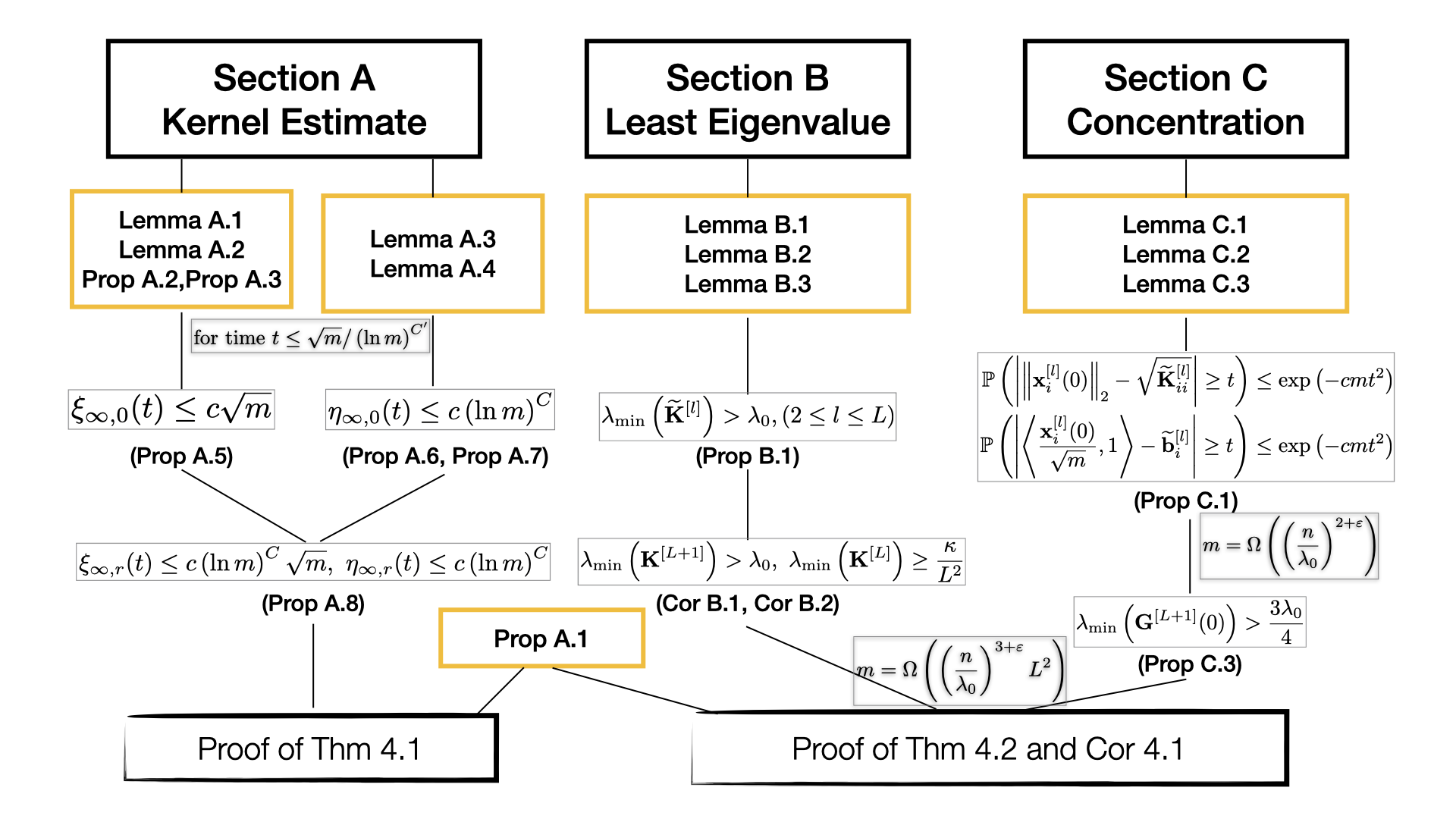
Figure 1: Diagram of the Proof of Main Theorems

Proof of Theorem 4.1.

Since each term in kernel $\mathcal{K}_{t}^{(r)}(\bm{x}_{\alpha_{1}},\bm{x}_{\alpha_{2}},\dots,\bm{x}_{\alpha_{r}}),$ it takes the form

$$\frac{1}{m^{r/2-1}}\prod_{j=1}^{s}\frac{\left<\bm{v}_{2j-1}(t),\bm{v}_{2j}(t)\right>}{m},\ 1\leq s\leq r,\ \ \bm{v}_{i}(t)\in\mathbb{A}_{0}\cup\mathbb{A}_{1}\cup\dots\cup\mathbb{A}_{r-2},$$

then for time $0\leq t\leq\sqrt{m}/{\left(\ln m\right)}^{C^{\prime}},$ $r\geq 3$

$$\left\lVert\mathcal{K}_{t}^{(2)}(\cdot)\right\rVert_{\infty} \lesssim\left(\frac{\xi_{\infty,0}(t)^{2}}{m}\right)^{2}\lesssim 1,$$

$$\left\lVert\mathcal{K}_{t}^{(r)}(\cdot)\right\rVert_{\infty} \lesssim\frac{1}{m^{r/2-1}}\left(\frac{\xi_{\infty,r}(t)^{2}}{m}\right)^{s}\lesssim\frac{1}{m^{r/2-1}}\left(\frac{\left(c{\left(\ln m\right)}^{C}\sqrt{m}\right)^{2}}{m}\right)^{r}\lesssim\frac{{\left(\ln m\right)}^{2rC}}{m^{r/2-1}}.$$

∎

Now we sketch the proofs for Theorem 4.2 and Corollary 4.1. Details can be found in Appendix D.

Sketch of the Proof of Theorem 4.2.

Since there exists $\frac{1}{L^{2}}$ scaling in some kernels, we use $C(r,L)$ to denote the ‘effective terms’ in each kernel. We denote $\mathcal{G}_{t}^{[L+1]}\left(\cdot\right)$ by $\mathcal{G}_{t}^{[2]}\left(\cdot\right),$ i.e., $\mathcal{G}_{t}^{(2)}(\cdot):=\mathcal{G}_{t}^{[L+1]}(\cdot),$ it’s natural for us to get that $C(2,L)=\mathcal{O}(1).$

Next, we apply the replacement rule, all the possible terms generated from $\mathcal{G}_{t}^{(2)}(\cdot)$ are

$$\mathcal{G}_{t}^{(2)}(\bm{x}_{\alpha_{1}},\bm{x}_{\alpha_{2}})=\left<\bm{x}_{\alpha_{1}}^{[L]},\bm{x}_{\alpha_{2}}^{[L]}\right>\to\mathcal{G}_{t}^{(3)}(\bm{x}_{\alpha_{1}},\bm{x}_{\alpha_{2}},\bm{x}_{\beta})$$

$$\mathcal{G}_{t}^{(3)}(\bm{x}_{\alpha_{1}},\bm{x}_{\alpha_{2}},\bm{x}_{\beta})={\frac{c_{\sigma}}{m}}\underbrace{\left<\mathrm{diag}\left(\bm{E}_{t,\alpha_{1}}^{[2:L]}\bm{\sigma}^{(1)}_{[1]}(\bm{x}_{\alpha_{1}})\bm{\sigma}^{(1)}_{[1]}(\bm{x}_{\beta})\left(\bm{E}_{t,\beta}^{[2:L]}\right)^{\intercal}\bm{a}_{t}\right)\bm{1},\bm{x}_{\alpha_{2}}^{[L]}\right>\left<\bm{x}_{\alpha_{1}},\bm{x}_{\beta}\right>}_{\textrm{I}}$$

$$+\sum_{k=2}^{L}\frac{c_{\mathrm{res}}^{2}}{L^{2}{m}}\underbrace{\left<\mathrm{diag}\left(\bm{E}_{t,\alpha_{1}}^{[(k+1):L]}\bm{\sigma}^{(1)}_{[k]}(\bm{x}_{\alpha_{1}})\bm{\sigma}^{(1)}_{[k]}(\bm{x}_{\beta})\left(\bm{E}_{t,\beta}^{[(k+1):L]}\right)^{\intercal}\bm{a}_{t}\right)\bm{1},\bm{x}_{\alpha_{2}}^{[L]}\right>\left<\bm{x}_{\alpha_{1}}^{[k-1]},\bm{x}_{\beta}^{[k-1]}\right>}_{\mathrm{II}}$$

$$+{\frac{c_{\sigma}}{m}}\left<\mathrm{diag}\left(\bm{E}_{t,\alpha_{2}}^{[2:L]}\bm{\sigma}^{(1)}_{[1]}(\bm{x}_{\alpha_{2}})\bm{\sigma}^{(1)}_{[1]}(\bm{x}_{\beta})\left(\bm{E}_{t,\beta}^{[2:L]}\right)^{\intercal}\bm{a}_{t}\right)\bm{1},\bm{x}_{\alpha_{1}}^{[L]}\right>\left<\bm{x}_{\alpha_{2}},\bm{x}_{\beta}\right>$$

$$+\sum_{k=2}^{L}\frac{c_{\mathrm{res}}^{2}}{L^{2}{m}}\left<\mathrm{diag}\left(\bm{E}_{t,\alpha_{2}}^{[(k+1):L]}\bm{\sigma}^{(1)}_{[k]}(\bm{x}_{\alpha_{2}})\bm{\sigma}^{(1)}_{[k]}(\bm{x}_{\beta})\left(\bm{E}_{t,\beta}^{[(k+1):L]}\right)^{\intercal}\bm{a}_{t}\right)\bm{1},\bm{x}_{\alpha_{1}}^{[L]}\right>\left<\bm{x}_{\alpha_{2}}^{[k-1]},\bm{x}_{\beta}^{[k-1]}\right>.$$

we have $C(3,L)=\mathcal{O}\left(2\left(1+\frac{L-1}{L^{2}}\right)\right)=\mathcal{O}\left(1+\frac{1}{L}\right).$

Finally for $\mathcal{G}_{t}^{(4)}(\cdot),$ by symmetry, we are only going to analyze terms I and II. Since there are at most $(2L+2)$ symbols in term I to be replaced, and by the replacement rules, each replacement will bring about up to $(L+1)$ many terms. For term II, for each summand, there are also at most $(2L+2)$ symbols to be replaced. Since there are $L-1$ summands in II, and each replacement will bring about up to $(L+1)$ many terms. we have that

$$C(4,L)=\mathcal{O}\left(2\left((2L+2)(L+1)+\frac{1}{L^{2}}(L-1)(2L+2)(L+1)\right)\right)=\mathcal{O}\left(L^{2}\right).$$

It holds that for time $0\leq t\leq\sqrt{m}/{\left(\ln m\right)}^{C^{\prime}}$

$$\left\lvert\partial_{t}\mathcal{G}_{t}^{(3)}\left(\bm{x}_{\alpha_{1}},\bm{x}_{\alpha_{2}},\bm{x}_{\alpha_{3}}\right)\right\rvert \leq\left\lVert\mathcal{G}_{t}^{(4)}(\cdot)\right\rVert_{\infty}\sqrt{R_{S}(\bm{\theta}_{0})}\leq C(4,L)\frac{{\left(\ln m\right)}^{C}}{m},$$

$$\left\lvert\mathcal{G}_{t}^{(3)}\left(\bm{x}_{\alpha_{1}},\bm{x}_{\alpha_{2}},\bm{x}_{\alpha_{3}}\right)\right\rvert \leq\left\lVert\mathcal{G}_{0}^{(3)}\left(\cdot\right)\right\rVert_{\infty}+tC(4,L)\frac{{\left(\ln m\right)}^{C}}{m}.$$

Finally, we need to make estimate on $\left\lVert\mathcal{G}_{0}^{(3)}\left(\cdot\right)\right\rVert_{\infty}.$ Each term in $\mathcal{G}_{0}^{(3)}\left(\cdot\right)$ is of the form $\frac{c}{m}\left<\bm{B}\bm{a}_{0},\bm{x}_{\alpha_{1}}^{[L]}\right>\left<\bm{x}_{\alpha_{2}}^{[l]},\bm{x}_{\beta}^{[l]}\right>$ where $\bm{B}$ is some specific matrix that changes from term to term. After taking conditional expectation up to the random variable $\bm{a}_{0},$ we have with high probability

$$\frac{c}{m}\left<\bm{a}_{0},\bm{B}^{\intercal}\bm{x}_{\alpha_{1}}^{[L]}\right>\left<\bm{x}_{\alpha_{2}}^{[l]},\bm{x}_{\beta}^{[l]}\right>\leq c\frac{{\left(\ln m\right)}^{C}}{m}.$$ (5.10)

Consequently, for time $0\leq t\leq\sqrt{m}/{\left(\ln m\right)}^{C^{\prime}}$

$$\left\lvert\mathcal{G}_{t}^{(3)}\left(\bm{x}_{\alpha_{1}},\bm{x}_{\alpha_{2}},\bm{x}_{\alpha_{3}}\right)\right\rvert \leq C(3,L)\frac{{\left(\ln m\right)}^{C}}{m}+tC(4,L)\frac{{\left(\ln m\right)}^{C}}{m},$$

$$\left\lvert\partial_{t}\mathcal{G}_{t}^{(2)}\left(\bm{x}_{\alpha_{1}},\bm{x}_{\alpha_{2}}\right)\right\rvert \leq\left\lVert\mathcal{G}_{t}^{(3)}(\cdot)\right\rVert_{\infty}\sqrt{R_{S}(\bm{\theta}_{0})}\leq\left(C(3,L)+tC(4,L)\right)\frac{{\left(\ln m\right)}^{C}}{m},$$

which finishes the proof of Theorem 4.2. ∎

Sketch of the Proof of Corollary 4.1.

If $m=\Omega\left(\left(\frac{n}{\lambda_{0}}\right)^{2+\varepsilon}\right)$, with high probability w.r.t random initialization, $\lambda_{\min}\left[\mathcal{K}_{0}^{(2)}\left(\bm{x}_{\alpha},\bm{x}_{\beta}\right)\right]_{1\leq\alpha,\beta\leq n}>\lambda_{\min}\left(\bm{G}^{[L+1]}(0)\right)>\frac{3\lambda_{0}}{4},$ by setting $\lambda=\frac{3\lambda_{0}}{4},$ we finish the proof of (4.12).

Concerning the change of the least eigenvalue of the NTK, from the Sketch Proof of Theorem 4.2, for time $0\leq t\leq\sqrt{m}/{\left(\ln m\right)}^{C^{\prime}},$

$$\left\lVert\left(\mathcal{G}_{t}^{(2)}-\mathcal{G}_{0}^{(2)}\right)(\cdot)\right\rVert_{2\to 2}\leq \left\lVert\left(\mathcal{G}_{t}^{(2)}-\mathcal{G}_{0}^{(2)}\right)(\cdot)\right\rVert_{\mathrm{F}}$$

$$\leq n \left\lVert\left(\mathcal{G}_{t}^{(2)}-\mathcal{G}_{0}^{(2)}\right)(\cdot)\right\rVert_{\infty}\leq nt\left(C(3,L)+tC(4,L)\right)\frac{{\left(\ln m\right)}^{C}}{m},$$

set $t^{*}$ satisfying :

$$C(4,L)(t^{*})^{2}+C(3,L)t^{*} =\frac{\lambda m}{2{\left(\ln m\right)}^{C}n},$$ (5.11)

after solving (5.11)

$$t^{*}=\frac{-C(3,L)+\sqrt{\left(C(3,L)\right)^{2}+2C(4,L)\frac{\lambda m}{{\left(\ln m\right)}^{C}n}}}{2C(4,L)}\geq\frac{1}{2}\sqrt{\frac{\lambda m}{C(4,L){\left(\ln m\right)}^{C}n}}.$$

Let $\bar{t}:=\inf\left\{t:\lambda_{\min}\left[\mathcal{K}_{t}^{(2)}\left(\bm{x}_{\alpha},\bm{x}_{\beta}\right)\right]_{1\leq\alpha,\beta\leq n}\geq\lambda/2\right\},$ naturally we have $t^{*}\leq\bar{t}.$ Using (4.6) we have for any $0\leq t\leq\bar{t},R_{S}(\bm{\theta}_{t})\leq\exp\left(-{\lambda t}/{n}\right)R_{S}(\bm{\theta}_{0}).$

Set $R_{S}(\bm{\theta}_{t})=\varepsilon$, it takes time $t\leq\left({n}/{\lambda}\right)\ln({R_{S}(\bm{\theta}_{0})}/{\varepsilon})$ for loss $R_{S}(\bm{\theta}_{t})$ to reach accuracy $\varepsilon,$ hence if $t\leq\left({n}/{\lambda}\right)\ln\left({R_{S}(\bm{\theta}_{0})}/{\varepsilon}\right)\leq t^{*}\leq\bar{t},$ then width $m$ is required to be

$$\frac{n}{\lambda}\ln\left(\frac{R_{S}(\bm{\theta}_{0})}{\varepsilon}\right)\leq\frac{1}{2}\sqrt{\frac{\lambda m}{C(4,L){\left(\ln m\right)}^{C}n}}.$$ (5.12)

thus we have

$$m\geq C(4,L)\left(\frac{n}{\lambda}\right)^{3}\left(\ln m\right)^{C}\ln\left(\frac{R_{S}(\bm{\theta}_{0})}{\varepsilon}\right)^{2},$$

since $C(4,L)=\mathcal{O}\left(L^{2}\right),$ we finish the proof. ∎

6 Discussion

In this paper, we show that the GD on ResNet can obtain zero training loss, and its training dynamic is given by an infinite hierarchy of ordinary differential equations, i.e., the NTH, which makes it possible to study the change of the NTK directly for deep neural networks. Our proof builds on a careful analysis of the least eigenvalue of randomly initialized Gram matrix, and the uniform upper bound on kernels of higher order in the NTH.

We list out some future directions for research:

• The NTH is an infinite sequence of relationship. However, Huang and Yau showed that under certain conditions on the width and the data set dimension, the NTH can be truncated and the truncated version of NTH is still able to approximate the original dynamic up to any precision. We believe that for ResNet, such technical conditions can be loosened based on our result.

• In Corollary 4.1, the dependence of $m$ on the depth $L$ is quadratic, we believe that the dependence can be reduced even further. We conjecture that $m$ is independent of $L.$

• In this paper, we focus on the GD, and we believe that it can be extended to SGD, while maintaining the linear convergence rate.

• We focus on the training loss, but does not address the test loss. To further investigate the generalization power of ResNet, we believe some Apriori estimate for the generalization error of ResNet may be useful [33].

Appendix A Estimates on the Kernel

A.1 Structure on Hierarchical Sets of Kernel Expressions

Since we have mentioned the replacement rules in Section 5.1, we haven’t rigorously justified it yet. Hence we use Proposition A.1 to shed light on the structures of the elements in $\mathbb{A}_{r}$, and consequently on the structures of each term in kernel $\mathcal{K}_{t}^{(r)}(\bm{x}_{\alpha_{1}},\bm{x}_{\alpha_{2}},\dots,\bm{x}_{\alpha_{r}})$.

Proposition A.1.

For any vector $\bm{v}(t)\in\mathbb{A}_{r}$, the new vector obtained from $\bm{v}(t)$ by performing the replacement rules are the sum of terms of the following forms:

$$(a).\frac{C}{\sqrt{m}} \bm{v}^{\prime}(t):\bm{v}^{\prime}(t)\in\mathbb{A}_{r},$$

$$(b).\frac{C}{\sqrt{m}} \bm{v}^{\prime}(t)\frac{\left<\bm{p},\bm{q}\right>}{m}:\bm{v}^{\prime}(t)\in\mathbb{A}_{r+1},\bm{p},\bm{q}\in\mathbb{A}_{0},$$

$$(c).\frac{C}{\sqrt{m}} \bm{v}^{\prime}(t)\frac{\left<\sqrt{m}\bm{x}_{\alpha},\sqrt{m}\bm{x}_{\beta}\right>}{m}:\bm{v}^{\prime}(t)\in\mathbb{A}_{r+1},\bm{p},\bm{q}\in\mathbb{A}_{0},$$

$$(d).\frac{C}{\sqrt{m}} \bm{v}^{\prime}(t)\frac{\left<\bm{p},\bm{q}\right>}{m}:\bm{v}^{\prime}(t)\in\mathbb{A}_{r-s+1},\bm{p}\in\mathbb{A}_{s},\bm{q}\in\mathbb{A}_{0},\ \text{for some }\ s\geq 1,$$

$$(e).\frac{C}{\sqrt{m}} \bm{v}^{\prime}(t)\frac{\left<\bm{p},\bm{q}\right>}{m}:\bm{v}^{\prime}(t)\in\mathbb{A}_{s},\bm{p}\in\mathbb{A}_{r-s+1},\bm{q}\in\mathbb{A}_{0},\ \text{for some}\ s\geq 1.$$

Proof.

The proof comes as follows. Note that the constant $C$ listed out below might keep changing from term to term.

Since $\bm{a}_{t}$ appears only at the position $\bm{e}_{0}$, if $\bm{v}(t)\in\mathbb{A}_{r},$ based on the replacement rule

$$\bm{v}(t)=\bm{e}_{s}\bm{e}_{s-1}\dots\bm{e}_{1}\bm{a}_{t}\to\widetilde{\bm{v}}(t)=\frac{1}{\sqrt{m}}\bm{e}_{s}\bm{e}_{s-1}\dots\bm{e}_{1}\sqrt{m}\bm{x}_{\beta}^{[L]}=\frac{1}{\sqrt{m}}\bm{v}^{\prime}(t),$$

then $\bm{v}^{\prime}(t)=\bm{e}_{s}\bm{e}_{s-1}\dots\bm{e}_{1}\sqrt{m}\bm{x}_{\beta}^{[L]}\in\mathbb{A}_{r}.$

Similarly, $\sqrt{m}\bm{x}_{\alpha}^{[l]}$ also appears only at $\bm{e}_{0}$, then if $\bm{v}(t)\in\mathbb{A}_{r},$ by the replacement rule

$$\bm{v}(t) =\bm{e}_{s}\bm{e}_{s-1}\dots\bm{e}_{1}\sqrt{m}\bm{x}_{\alpha}^{[l]}\to\widetilde{\bm{v}}(t),$$

$$\widetilde{\bm{v}}(t) =\sum_{k}\frac{C}{\sqrt{m}}\bm{e}_{s}\bm{e}_{s-1}\dots\bm{e}_{1}\ \mathrm{diag}(\bm{f}_{k})\bm{1}\frac{\left<\sqrt{m}\bm{x}_{\alpha}^{[k]},\sqrt{m}\bm{x}_{\beta}^{[k]}\right>}{m}=\sum_{k}\frac{C}{\sqrt{m}}\bm{v}^{\prime}_{k}(t)\frac{\left<\sqrt{m}\bm{x}_{\alpha}^{[k]},\sqrt{m}\bm{x}_{\beta}^{[k]}\right>}{m},$$

given that $\bm{f}_{k}\in\mathbb{A}_{0},$ then $\bm{v}^{\prime}_{k}(t)\in\mathbb{A}_{r+1}.$

Since $\bm{\sigma}_{[l]}^{(u)}(\bm{x}_{\alpha})$ only appears at the starting or the middle position, i.e., $\bm{e}_{j},\ j\geq 1$. For $u=1,$ $\bm{\sigma}_{[l]}^{(1)}(\bm{x}_{\alpha})$ has no diag operations accompanied with it, and any vector $\bm{v}(t)\in\mathbb{A}_{r}$ could contain $\bm{\sigma}_{[l]}^{(1)}(\bm{x}_{\alpha}),$ for $r\geq 0$

$$\bm{v}(t) =\bm{e}_{s}\dots\bm{e}_{j+1}\bm{\sigma}_{[l]}^{(1)}(\bm{x}_{\alpha})\bm{e}_{j-1}\dots\bm{e}_{0}\to\widetilde{\bm{v}}(t),$$

$$\widetilde{\bm{v}}(t) =\frac{C}{\sqrt{m}}\bm{e}_{s}\dots\bm{e}_{j+1}\bm{\sigma}_{[l]}^{(2)}(\bm{x}_{\alpha})\mathrm{diag}\left(\bm{f}_{1}\right)\bm{e}_{j-1}\dots\bm{e}_{0}\frac{\left<\bm{p}_{1},\bm{q}_{1}\right>}{m}$$

$$+\sum_{k}\frac{C}{\sqrt{m}}\bm{e}_{s}\dots\bm{e}_{j+1}\bm{\sigma}_{[l]}^{(2)}(\bm{x}_{\alpha})\mathrm{diag}\left(\frac{\bm{W}_{t}^{[l]}}{\sqrt{m}}\bm{f}_{k}\right)\bm{e}_{j-1}\dots\bm{e}_{0}\frac{\left<\bm{p}_{k},\bm{q}_{k}\right>}{m}$$

$$=\sum_{l}\frac{C}{\sqrt{m}}\bm{v}^{\prime}_{l}(t)\frac{\left<\bm{p}_{l},\bm{q}_{l}\right>}{m},$$

since $\bm{f}_{k}\in\mathbb{A}_{0},$ then $\bm{v}^{\prime}_{l}(t)\in\mathbb{A}_{r+1},$ and $\bm{p}_{l},\bm{q}_{l}\in\mathbb{A}_{0}.$

For $u\neq 1,$ $\bm{\sigma}_{[l]}^{(u)}(\bm{x}_{\alpha})$ has at most $u-1$ diag operations behind it, and only vector $\bm{v}(t)\in\mathbb{A}_{r}$ could contain $\bm{\sigma}_{[l]}^{(u)}(\bm{x}_{\alpha}),$ for $r\geq u-1.$

$$\bm{v}(t) =\bm{e}_{s}\dots\bm{e}_{j+1}\bm{e}_{j}\bm{e}_{j-1}\dots\bm{e}_{0}\to\widetilde{\bm{v}}(t),$$

$$\text{with}\ \bm{e}_{j} =\bm{\sigma}_{[l]}^{(u)}(\bm{x}_{\alpha})\mathrm{diag}\left(\left(\frac{\bm{W}_{t}^{[l]}}{\sqrt{m}}\right)^{Q_{1}}\bm{g}_{1}\right)\dots\mathrm{diag}\left(\left(\frac{\bm{W}_{t}^{[l]}}{\sqrt{m}}\right)^{Q_{u-1}}\bm{g}_{u-1}\right)\left(\frac{c_{\mathrm{res}}}{L}\frac{\bm{W}_{t}^{[l]}}{\sqrt{m}}\right)^{Q_{u}},$$

$$\text{or}\ \bm{e}_{j} =\left(\frac{c_{\mathrm{res}}}{L}\frac{\left(\bm{W}_{t}^{[l]}\right)^{\intercal}}{\sqrt{m}}\right)^{Q_{u}}\bm{\sigma}_{[l]}^{(u)}(\bm{x}_{\alpha})\mathrm{diag}\left(\left(\frac{\bm{W}_{t}^{[l]}}{\sqrt{m}}\right)^{Q_{1}}\bm{g}_{1}\right)\dots\mathrm{diag}\left(\left(\frac{\bm{W}_{t}^{[l]}}{\sqrt{m}}\right)^{Q_{u-1}}\bm{g}_{u-1}\right),$$

and after applying replacement rules on $\bm{e}_{j}\to\bm{e}_{j}^{{}^{\prime}}$,

$$\bm{e}_{j}^{{}^{\prime}} =\frac{C}{\sqrt{m}}\bm{\sigma}_{[l]}^{(u+1)}(\bm{x}_{\alpha})\mathrm{diag}\left(\bm{f}_{1}\right)\mathrm{diag}\left(\left(\frac{\bm{W}_{t}^{[l]}}{\sqrt{m}}\right)^{Q_{1}}\bm{g}_{1}\right)\dots\left(\frac{c_{\mathrm{res}}}{L}\frac{\bm{W}_{t}^{[l]}}{\sqrt{m}}\right)^{Q_{u}}\frac{\left<\bm{p}_{1},\bm{q}_{1}\right>}{m}$$

$$+ \sum_{k}\frac{C}{\sqrt{m}}\bm{\sigma}_{[l]}^{(u+1)}(\bm{x}_{\alpha})\mathrm{diag}\left(\left(\frac{\bm{W}_{t}^{[l]}}{\sqrt{m}}\right)^{Q_{0}}\bm{f}_{k}\right)\mathrm{diag}\left(\left(\frac{\bm{W}_{t}^{[l]}}{\sqrt{m}}\right)^{Q_{1}}\bm{g}_{1}\right)\dots\left(\frac{c_{\mathrm{res}}}{L}\frac{\bm{W}_{t}^{[l]}}{\sqrt{m}}\right)^{Q_{u}}\frac{\left<\bm{p}_{k},\bm{q}_{k}\right>}{m},$$

$$\text{or}\ \bm{e}_{j}^{{}^{\prime}} =\frac{C}{\sqrt{m}}\left(\frac{c_{\mathrm{res}}}{L}\frac{\left(\bm{W}_{t}^{[l]}\right)^{\intercal}}{\sqrt{m}}\right)^{Q_{u}}\bm{\sigma}_{[l]}^{(u+1)}(\bm{x}_{\alpha})\mathrm{diag}\left(\bm{f}_{1}\right)\dots\mathrm{diag}\left(\left(\frac{\bm{W}_{t}^{[l]}}{\sqrt{m}}\right)^{Q_{u-1}}\bm{g}_{u-1}\right)\frac{\left<\bm{p}_{1},\bm{q}_{1}\right>}{m}$$

$$+\sum_{k} \frac{C}{\sqrt{m}}\left(\frac{c_{\mathrm{res}}}{L}\frac{\left(\bm{W}_{t}^{[l]}\right)^{\intercal}}{\sqrt{m}}\right)^{Q_{u}}\bm{\sigma}_{[l]}^{(u+1)}(\bm{x}_{\alpha})\mathrm{diag}\left(\left(\frac{\bm{W}_{t}^{[l]}}{\sqrt{m}}\right)^{Q_{0}}\bm{f}_{k}\right)\dots\mathrm{diag}\left(\left(\frac{\bm{W}_{t}^{[l]}}{\sqrt{m}}\right)^{Q_{u-1}}\bm{g}_{u-1}\right)\frac{\left<\bm{p}_{k},\bm{q}_{k}\right>}{m},$$

then

$$\widetilde{\bm{v}}(t)=\sum_{l}\frac{C}{\sqrt{m}}\bm{v}^{\prime}_{l}(t)\frac{\left<\bm{p}_{l},\bm{q}_{l}\right>}{m},$$

since $\bm{f}_{k}\in\mathbb{A}_{0},$ then $\bm{v}^{\prime}_{l}(t)\in\mathbb{A}_{r+1},$ and $\bm{p}_{l},\bm{q}_{l}\in\mathbb{A}_{0}.$

Since $\frac{\bm{W}_{t}^{[l]}}{\sqrt{m}}$ only appears at the starting or the middle position $\bm{e}_{j}$, we have that if $\bm{v}(t)\in\mathbb{A}_{r},$ then based on the replacement rules

$$\bm{v}(t) =\bm{e}_{s}\bm{e}_{s-1}\dots\bm{e}_{j+1}\frac{\bm{W}_{t}^{[l]}}{\sqrt{m}}\bm{e}_{j-1}\dots\bm{e}_{1}\bm{e}_{0}\to\widetilde{\bm{v}}(t),$$

$$\widetilde{\bm{v}}(t) =\frac{C}{{m}}\bm{e}_{s}\bm{e}_{s-1}\dots\bm{e}_{j+1}\mathrm{diag}(\bm{g})\ \bm{1}\otimes(\bm{x}^{[l-1]}_{\beta})^{\intercal}\bm{e}_{j-1}\dots\bm{e}_{1}\bm{e}_{0}$$

$$=\frac{C}{\sqrt{m}}\bm{e}_{s}\bm{e}_{s-1}\dots\bm{e}_{j+1}\mathrm{diag}(\bm{g})\ \bm{1}\frac{\left<\bm{e}_{j-1}\dots\bm{e}_{1}\bm{e}_{0},\sqrt{m}\bm{x}_{\beta}^{[l-1]}\right>}{m}$$

$$=\frac{C}{\sqrt{m}}\bm{v}^{\prime}(t)\frac{\left<\bm{p},\bm{q}\right>}{m},$$

with $\bm{v}^{\prime}(t)\in\mathbb{A}_{r-s+1},$ and $\bm{p}\in\mathbb{A}_{s},\bm{q}\in\mathbb{A}_{0},$ for some $s\geq 1.$

Similarly for $\frac{(\bm{W}_{t}^{[l])^{\intercal}}}{\sqrt{m}},$

$$\bm{v}(t) =\bm{e}_{s}\bm{e}_{s-1}\dots\bm{e}_{j+1}\frac{(\bm{W}_{t}^{[l]})^{\intercal}}{\sqrt{m}}\bm{e}_{j-1}\dots\bm{e}_{1}\bm{e}_{0}\to\widetilde{\bm{v}}(t)$$

$$\widetilde{\bm{v}}(t) =\frac{C}{{m}}\bm{e}_{s}\bm{e}_{s-1}\dots\bm{e}_{j+1}\bm{x}_{\beta}^{[l-1]}\ \otimes\bm{1}^{\intercal}\mathrm{diag}(\bm{g})\bm{e}_{j-1}\dots\bm{e}_{1}\bm{e}_{0}$$

$$=\frac{C}{\sqrt{m}}\bm{e}_{s}\bm{e}_{s-1}\dots\bm{e}_{j+1}\sqrt{m}\bm{x}_{\beta}^{[l-1]}\ \frac{\left<\mathrm{diag}(\bm{g})\bm{e}_{j-1}\dots\bm{e}_{1}\bm{e}_{0},\bm{1}\right>}{m}$$

$$=\frac{C}{\sqrt{m}}\bm{v}^{\prime}(t)\frac{\left<\bm{p},\bm{q}\right>}{m},$$

with $\bm{v}^{\prime}(t)\in\mathbb{A}_{r-s},$ and $\bm{p}\in\mathbb{A}_{r-s+1},\bm{q}\in\mathbb{A}_{0},$ for some $s\geq 1.$ Since $\bm{E}_{t,\alpha}^{[l]}$ is situations combined with $\frac{\bm{W}_{t}^{[l]}}{\sqrt{m}}$ and $\bm{\sigma}_{[l]}^{(1)}(\bm{x}_{\alpha}),$ so we will skip the analysis. ∎

From the discussion above, if we apply Proposition A.1 to $\mathcal{K}_{t}^{(r)}(\bm{x}_{\alpha_{1}},\bm{x}_{\alpha_{2}})$ inductively $(r-1)$ times, for each term in kernel $\mathcal{K}_{t}^{(r)}(\bm{x}_{\alpha_{1}},\bm{x}_{\alpha_{2}},\dots,\bm{x}_{\alpha_{r}})$, it takes the form:

$$\frac{1}{m^{r/2-1}}\prod_{j=1}^{s}\frac{\left<\bm{v}_{2j-1}(t),\bm{v}_{2j}(t)\right>}{m},\ 1\leq s\leq r,\ \ \bm{v}_{i}(t)\in\mathbb{A}_{0}\cup\mathbb{A}_{1}\cup\dots\cup\mathbb{A}_{r-2}.$$ (A.1)

A.2 Apriori $L^{2}$ bounds for expressions in $\mathbb{A}_{0}$

We begin with an estimate on the empirical risk $R_{S}(\bm{\theta}_{t})$.

Proposition A.2.

Under Assumption 4.1 and 4.2, we have for $t\geq 0,$

$$R_{S}(\bm{\theta}_{t})\leq R_{S}(\bm{\theta}_{0})\sim\mathcal{O}(1).$$ (A.2)

Proof.

We get inequality (A.2) by non-negative definiteness of kernel $\mathcal{K}_{t}^{(2)}(\cdot)$. From (4.6), we obtain that

$$\partial_{t}\sum_{\alpha=1}^{n}\left\lVert f_{\alpha}(t)-y_{\alpha}\right\rVert_{2}^{2}=-\frac{2}{n}\sum_{\alpha,\beta=1}^{n}\mathcal{K}_{t}^{(2)}(\bm{x}_{\alpha},\bm{x}_{\beta})(f_{\alpha}(t)-y_{\alpha})(f_{\beta}(t)-t_{\beta})\leq 0,$$ (A.3)

hence

$$R_{S}(\bm{\theta}_{t})\leq R_{S}(\bm{\theta}_{0}),$$

which finish the proof of Proposition A.2. ∎

Our next proposition is mainly on the spectral property of the skip-connection matrices. This proposition is similar to Proposition $\mathrm{B.1.}$ in [23].

Proposition A.3.

Under Assumptions 4.1 and 4.2, we define $\xi(t)$ as follows

$$\xi(t)=\sup_{0\leq t^{\prime}\leq t}\max\Bigg{\{}1,\frac{1}{\sqrt{m}}\Big{\{} \left\lVert\bm{W}_{t^{\prime}}^{[2]}\right\rVert_{2\to 2},\left\lVert\left(\bm{W}_{t^{\prime}}^{[2]}\right)^{\intercal}\right\rVert_{2\to 2},\dots$$

$$\dots, \left\lVert\bm{W}_{t^{\prime}}^{[L]}\right\rVert_{2\to 2},\left\lVert\left(\bm{W}_{t^{\prime}}^{[L]}\right)^{\intercal}\right\rVert_{2\to 2},\left\lVert\bm{a}_{t^{\prime}}\right\rVert_{2}\Big{\}}\Bigg{\}},$$ (A.4)

then with high probability w.r.t the random initialization, for $t\lesssim\sqrt{m}$

$$\xi(t)\leq c_{w,t}.$$ (A.5)

where $c_{w,t}>2$ is a constant independent of the depth of the network $L$.

Moreover for $t\lesssim\sqrt{m}$, $c_{w,t}$ has a uniform upper bound in $t,$ i.e.,

$$c_{w,t}\leq\bar{c},$$ (A.6)

where $\bar{c}$ is independent of depth $L$ and time $t.$

Proof.

For the purpose of proving the proposition, we shall state two lemmas, Lemma A.1 and A.2. Lemma A.1 is given out as Lemma $\mathrm{G}.2.$ in Du et al.[13], also consequence of the results in [45].

Lemma A.1.

Given a matrix $\bm{W}\in\mathbb{R}^{m\times m}$ with each entry $W_{i,j}\sim\mathcal{N}(0,1),$ then with probability at least $1-\exp\left(-\frac{(c^{{}^{\prime}}_{w,0}-2)^{2}m}{2}\right),$ the following holds

$$\left\lVert\bm{W}\right\rVert_{2\to 2}\leq{c^{{}^{\prime}}_{w,0}}\sqrt{m},$$ (A.7)

where $c^{{}^{\prime}}_{w,0}>2$ is a constant.

Remark A.1.

This event is an event that holds with high probability.

Next concerning the term $\frac{1}{\sqrt{m}}\left\lVert\bm{a}_{0}\right\rVert_{2}$, we shall state a lemma on the tail bound of the chi-square distribution, using Lemma 1 from [28]

Lemma A.2.

If $Z\sim\chi^{2}(m)$, then we have a tail bound

$$\mathbb{P}\left(Z\geq m+2\sqrt{mx}+2x\right)\leq e^{-x}.$$ (A.8)

Remark A.2.

This event is also an event that holds with high probability.

Then if we write $2tm=m+(2t-1)m$, letting $x=\frac{mt}{10},$ we can obtain that

$$\mathbb{P}\left(\left\lVert\bm{a}_{0}\right\rVert_{2}^{2}\geq m+2m\left(\sqrt{t/10}+t/10\right)\right)\leq\exp(-tm/10)),$$

and for $t\geq 1$, we have $2t-1\geq 2\left(\sqrt{t/10}+t/10\right).$ Thus, if we choose $t$ properly, we see that such event

$$\frac{1}{\sqrt{m}}\left\lVert\bm{a}_{0}\right\rVert_{2}\leq c^{{}^{\prime\prime}}_{w,0}$$

holds with high probability. Hence, for $t=0,$ $\xi(0)\leq\max\left\{1,c^{{}^{\prime}}_{w,0},c^{{}^{\prime\prime}}_{w,0}\right\}.$ We set $c_{w,0}$ as $c_{w,0}=\max\left\{1,c^{{}^{\prime}}_{w,0},c^{{}^{\prime\prime}}_{w,0}\right\},$ then

$$\xi(0)\leq c_{w,0}.$$ (A.9)

In the following we are going to show the upper bound of $\partial_{t}\xi(t).$ In order to do that, we need to estimate $L^{2}$ bound on each output layer. For $l=1,$

$$\left\lVert\bm{x}^{[1]}\right\rVert_{2} =\sqrt{\frac{c_{\sigma}}{{m}}}\left\lVert\sigma(\bm{W}_{t}^{[1]}\bm{x})\right\rVert_{2}\leq\sqrt{c_{\sigma}}\left(\left\lvert\sigma(0)\right\rvert+\frac{C_{L}}{\sqrt{m}}\left\lVert\bm{W}_{t}^{[1]}\bm{x}\right\rVert_{2}\right)$$

$$\leq\sqrt{c_{\sigma}}C_{L}\left(1+\xi(t)\left\lVert\bm{x}\right\rVert_{2}\right)\leq C\xi(t),$$ (A.10)

and for $2\leq l\leq L,$

$$\left\lVert\bm{x}^{[l]}\right\rVert_{2} \leq\left\lVert\bm{x}^{[l-1]}\right\rVert_{2}+\frac{c_{\mathrm{res}}}{L\sqrt{m}}\left\lVert\sigma\left(\bm{W}_{t}^{[l]}\bm{x}^{[l-1]}\right)\right\rVert_{2}$$

$$\leq\left\lVert\bm{x}^{[l-1]}\right\rVert_{2}+\frac{c_{\mathrm{res}}}{L}\left(\left\lvert\sigma(0)\right\rvert+C_{L}\xi(t)\left\lVert\bm{x}^{[l-1]}\right\rVert_{2}\right)$$

$$\leq\left\lVert\bm{x}^{[l-1]}\right\rVert_{2}+\frac{c_{\mathrm{res}}}{L}\left(C_{L}+C_{L}\xi(t)\left\lVert\bm{x}^{[l-1]}\right\rVert_{2}\right)$$

$$\leq\left(1+\frac{2c_{\mathrm{res}}}{L}\xi(t)\right)\left\lVert\bm{x}^{[l-1]}\right\rVert_{2}.$$ (A.11)

Hence we can obtain an inductive relation on the $2$-norm of $\bm{x}^{[l]}.$

$$\left\lVert\bm{x}^{[l]}\right\rVert_{2}\leq C\left(1+\frac{2c_{\mathrm{res}}}{L}\xi(t)\right)^{l-1}\xi(t).$$ (A.12)

Based on (3.7), (3.8), (3.9) and (3.10),  combined with Proposition A.2

$$\partial_{t}\left\lVert\bm{W}_{t}^{[l]}\right\rVert_{2\to 2} \leq\frac{1}{n}\sum_{\beta=1}^{n}\frac{C}{\sqrt{m}}\left\lVert\bm{\sigma}^{(1)}_{[l]}(\bm{x}_{\beta})\left(\bm{E}_{t,\beta}^{[(l+1):L]}\right)^{\intercal}\bm{a}_{t}\right\rVert_{2}\left\lVert\bm{x}_{\beta}^{[l-1]}\right\rVert_{2}\left\lvert f_{\beta}(t)-y_{\beta}\right\rvert$$

$$\leq\frac{1}{n}\sum_{\beta=1}^{n}{CC_{L}}\left(1+\frac{c_{\mathrm{res}}C_{L}}{L}\xi(t)\right)^{L-l}\xi(t)\left(1+\frac{2c_{\mathrm{res}}}{L}\xi(t)\right)^{l-1}\xi(t)\left\lvert f_{\beta}(t)-y_{\beta}\right\rvert$$

$$\leq C\left(1+\frac{2c_{\mathrm{res}}}{L}\xi(t)\right)^{L-1}\xi(t)^{2}\sqrt{\frac{1}{n}\sum_{\beta=1}^{n}\left\lVert f_{\beta}(t)-y_{\beta}\right\rVert_{2}^{2}}$$

$$\leq C\left(1+\frac{2c_{\mathrm{res}}}{L}\xi(t)\right)^{L-1}\xi(t)^{2}\sqrt{R_{S}\left(\bm{\theta}_{0}\right)}$$

$$\leq C\left(1+\frac{2c_{\mathrm{res}}}{L}\xi(t)\right)^{L-1}\xi(t)^{2}\leq C\exp\left(2c_{\mathrm{res}}\xi(t)\right)\ \xi(t)^{2},$$ (A.13)

$$\partial_{t}\left\lVert\bm{a}_{t}\right\rVert_{2} \leq\frac{1}{n}\sum_{\beta=1}^{n}\left\lVert\bm{x}_{\beta}^{[L]}\right\rVert_{2}\left\lvert f_{\beta}(t)-y_{\beta}\right\rvert\leq C\left(1+\frac{2c_{\mathrm{res}}}{L}\xi(t)\right)^{L-1}\xi(t)\sqrt{\frac{1}{n}\sum_{\beta=1}^{n}\left\lVert f_{\beta}(t)-y_{\beta}\right\rVert_{2}^{2}}$$

$$\leq C\left(1+\frac{2c_{\mathrm{res}}}{L}\xi(t)\right)^{L-1}\xi(t)\sqrt{R_{S}\left(\bm{\theta}_{0}\right)}$$

$$\leq C\left(1+\frac{2c_{\mathrm{res}}}{L}\xi(t)\right)^{L-1}\xi(t)\leq C\exp(2c_{\mathrm{res}}\xi(t))\ \xi(t).$$ (A.14)

Based on (A.13) and (A.14), we have

$$\sqrt{m}\ \partial_{t}\xi(t)\leq C\exp(2c_{\mathrm{res}}\xi(t))\xi^{2}(t),$$

we can obtain an integration inequality,

$$\int_{\xi(0)}^{\xi(t)}\frac{\mathop{}\!\mathrm{d}u}{\exp(2c_{\mathrm{res}}u)u^{2}}\leq\frac{Ct}{\sqrt{m}}.$$ (A.15)

Hence the integration term on the LHS of (A.15) is

$$\int_{\xi(0)}^{\xi(t)}\frac{\mathop{}\!\mathrm{d}u}{\exp(2c_{\mathrm{res}}u)u^{2}} \geq\frac{1}{\exp(2c_{\mathrm{res}}\xi(t))}\int_{\xi(0)}^{\xi(t)}\frac{\mathop{}\!\mathrm{d}u}{u^{2}}$$

$$=\frac{1}{\exp((2c_{\mathrm{res}}\xi(t))}\left(\frac{1}{\xi(0)}-\frac{1}{\xi(t)}\right)$$

$$\geq\frac{1}{\exp(2c_{\mathrm{res}}\xi(t))}\left(\frac{1}{c_{w,0}}-\frac{1}{\xi(t)}\right).$$

We shall notice for the single variable function $f(z)$

$$f(z)=\frac{1}{\exp(2c_{\mathrm{res}}z)}(\frac{1}{c_{w,0}}-\frac{1}{z}),$$

maximum of $f(z)$ can be achieved at point

$$z_{0}=\frac{c_{w,0}+\sqrt{c_{w,0}^{2}+2{c_{w,0}}/{c_{\mathrm{res}}}}}{2},$$

and $f(z)$ is monotone increasing in the interval $\left[c_{w,0},z_{0}\right].$ Thus, if we choose time $t$ properly, say $t\leq c\sqrt{m}$, $c$ being small enough, the following holds

$$\xi(t)\leq\frac{c_{w,0}+\sqrt{c_{w,0}^{2}+2{c_{w,0}}/{c_{\mathrm{res}}}}}{2}.$$

In other words, if $t\leq c\sqrt{m}$ for some small enough $c>0,$ we have

$$\xi(t)\leq c_{w,t}\leq\frac{c_{w,0}+\sqrt{c_{w,0}^{2}+2{c_{w,0}}/{c_{\mathrm{res}}}}}{2},$$

where the last quantity is independent of depth $L$ and time $t$, and we denote this by

$$\bar{c}=\frac{c_{w,0}+\sqrt{c_{w,0}^{2}+2{c_{w,0}}/{c_{\mathrm{res}}}}}{2},$$

which finishes the proof of Proposition A.3. ∎

We state the inductive relation (A.12) as a proposition.

Proposition A.4.

Under Assumptions 4.1 and 4.2, we have with high probability w.r.t the random initialization, for time $t\lesssim\sqrt{m}$ with $0\leq l\leq L,$

$$\left\lVert\bm{x}^{[l]}\right\rVert_{2}\leq C,$$ (A.16)

where $C>0$ is a constant, independent of depth $L$.

Remark A.3.

We shall note that the constant $C$ in Proposition A.4 only depends on $c_{\mathrm{res}},c_{w,0}$ and $c_{\sigma}.$ However, for a fully-connected feedforward network, (A.16) in Proposition A.4 become

$$\left\lVert\bm{x}^{[l]}\right\rVert_{2}\leq C\ 2^{l}.$$ (A.17)

Note that the $2$-norm for each output layer increase exponentially layer by layer for fully-connected network, showing that ResNet possesses more stability compared with fully-connected network.

Next we end this part by making an Apriori estimate on the $L^{2}$-norm for arbitrary vector $\bm{v}(t)\in\mathbb{A}_{0}.$

Proposition A.5.

Under Assumption 4.1 and 4.2, with high probability w.r.t the random initialization, uniformly for any vector $\bm{v}(t)\in\mathbb{A}_{0}$ and time $t\lesssim\sqrt{m},$ the following holds

$$\left\lVert\bm{v}(t)\right\rVert_{2}\leq c\sqrt{m},$$ (A.18)

where $c>0$ is a constant independent of depth $L$ and time $t$.

Proof.

We shall start our analysis on the whole expressions in set $\mathbb{A}_{0}.$ For any vector $\bm{v}(t)\in\mathbb{A}_{0},$ we can write $\bm{v}(t)=\bm{e}_{s}\bm{e}_{s-1}\dots\bm{e}_{1}\bm{e}_{0}$ with $0\leq s\leq 4L.$

We start with the estimate on $\bm{e}_{0},$ since $\bm{e}_{0}$ is chosen following the rules:

$$\bm{e}_{0}\in\left\{\bm{a}_{t},\{\sqrt{m}\bm{x}_{\beta}^{[1]},\sqrt{m}\bm{x}_{\beta}^{[2]},\dots,\sqrt{m}\bm{x}_{\beta}^{[L]}\}_{1\leq\beta\leq n}\right\}.$$

• (a). If $\bm{e}_{0}=\bm{a}_{t},$ then by Lemma A.2, for $t\lesssim\sqrt{m}$

  $$\left\lVert\bm{a}_{t}\right\rVert_{2}\leq c_{w,t}\sqrt{m}\leq c\sqrt{m}.$$

• (b). If $\bm{e}_{0}=\sqrt{m}\bm{x}_{\beta}^{[l]}$ where $1\leq l\leq L,$ then based on Proposition A.4, for $t\lesssim\sqrt{m}$

  $$\left\lVert\sqrt{m}\bm{x}_{\beta}^{[l]}\right\rVert_{2}=\sqrt{m}\left\lVert\bm{x}_{\beta}^{[l]}\right\rVert_{2}\leq c\sqrt{m}.$$

Now we proceed to other terms in the expression $\bm{e}_{j}$ where $j\geq 1.$

• (i). If $\bm{e}_{j}=\bm{\sigma}_{[l]}^{(1)}(\bm{x}_{\beta}),$ then we have

  $$\left\lVert\bm{v}(t)\right\rVert_{2} =\left\lVert\bm{e}_{s}\bm{e}_{s-1}\dots\bm{e}_{1}\bm{e}_{0}\right\rVert_{2}$$

  $$=\left\lVert\bm{e}_{s}\right\rVert_{2\to 2}\left\lVert\bm{e}_{s-1}\right\rVert_{2\to 2}\dots\left\lVert\bm{e}_{1}\right\rVert_{2\to 2}\left\lVert\bm{e}_{0}\right\rVert_{2}.$$

  Since $\left\lVert\bm{\sigma}_{[l]}^{(1)}(\bm{x}_{\beta})\right\rVert_{2\to 2}\leq C_{L}\leq 1,$ thus for all $j\geq 1$ with $\bm{e}_{j}=\bm{\sigma}_{[l]}^{(1)}(\bm{x}_{\beta})$

  $$\left\lVert\bm{v}(t)\right\rVert_{2}\leq\left(C_{L}\right)^{4L}c\sqrt{m}\leq c\sqrt{m}.$$

• (ii). If $\bm{e}_{j}=\bm{E}_{t,\beta}^{[l]}$ or $\bm{e}_{j}=\left(\bm{E}_{t,\beta}^{[l]}\right)^{\intercal},$ then based on Proposition A.3

  $$\left\lVert\bm{v}(t)\right\rVert_{2} =\left\lVert\bm{e}_{s}\right\rVert_{2\to 2}\left\lVert\bm{e}_{s-1}\right\rVert_{2\to 2}\dots\left\lVert\bm{e}_{1}\right\rVert_{2\to 2}\left\lVert\bm{e}_{0}\right\rVert_{2}.$$

  Since

  $$\left\lVert\bm{E}_{t,\beta}^{[l]}\right\rVert_{2\to 2}=\left\lVert\left(\bm{E}_{t,\beta}^{[l]}\right)^{\intercal}\right\rVert_{2\to 2}\leq\left(1+\frac{c_{\mathrm{res}}C_{L}}{L}\xi(t)\right)\leq\left(1+\frac{c_{\mathrm{res}}c_{w,t}}{L}\right),$$

  thus for all $j\geq 1$ with $\bm{e}_{j}=\bm{E}_{t,\beta}^{[l]}$ or $\bm{e}_{j}=\left(\bm{E}_{t,\beta}^{[l]}\right)^{\intercal},$

  $$\left\lVert\bm{v}(t)\right\rVert_{2} \leq\left(1+\frac{c_{\mathrm{res}}c_{w,t}}{L}\right)^{s}\left\lVert\bm{e}_{0}\right\rVert_{2},$$

  then by taking supreme on $0\leq s\leq 4L,$ we have

  $$\left\lVert\bm{v}(t)\right\rVert_{2} \leq\left(1+\frac{c_{\mathrm{res}}c_{w,t}}{L}\right)^{4L}\left\lVert\bm{e}_{0}\right\rVert_{2}$$

  $$\leq c\exp(4c_{\mathrm{res}}c_{w,t})\sqrt{m}\leq c\sqrt{m}.$$

Combining these two observations, we finish the proof. ∎

Thus, if we define the quantity $\xi_{\infty,0}(t)$ as follows,

$$\xi_{\infty,0}(t)=\sup_{0\leq t^{\prime}\leq t}\left\{\left\lVert\bm{v}(t^{\prime})\right\rVert_{2}:\bm{v}(t^{\prime})\in\mathbb{A}_{0}\right\}.$$ (A.19)

Then directly from Proposition A.5, for time $0\leq t\leq\sqrt{m}/{\left(\ln m\right)}^{C^{\prime}},$ the following holds

$$\xi_{\infty,0}(t)\leq c\sqrt{m}.$$ (A.20)

A.3 Apriori $L^{\infty}$ bounds for expressions in $\mathbb{A}_{0}$

In this part, we shall make estimate on the quantity $\eta_{\infty,0}(t)$ defined below

$$\eta_{\infty,0}(t)=\sup_{0\leq t^{\prime}\leq t}\left\{\left\lVert\bm{v}(t^{\prime})\right\rVert_{\infty}:\bm{v}(t^{\prime})\in\mathbb{A}_{0}\right\}.$$ (A.21)

We shall begin by a lemma on the $\left\lVert\cdot\right\rVert_{\infty}$ norm of a standard Gaussian vector.

Lemma A.3.

For any i.i.d. normal distribution $X_{1},X_{2},\dots,X_{m}\sim\mathcal{N}(0,1),$ it holds with high probability that the $L^{\infty}$-norm of the gaussian vector $\bm{X}=\left(X_{1},X_{2},\dots,X_{m}\right)^{\intercal}$ is upper bounded by

$$\left\lVert\bm{X}\right\rVert_{\infty}\leq{\left(\ln m\right)}^{C},$$

for some really large constant $C>0$ .

Proof.

For any $X_{i}\sim\mathcal{N}(0,1)$, we have that for some $\varepsilon,\lambda>0$

$$\mathbb{P}\left(X_{i}\geq\varepsilon\right) =\mathbb{P}\left(\exp\left(\lambda X_{i}\right)\geq\exp\left(\lambda\varepsilon\right)\right)$$

$$\leq\frac{\mathbb{E}\left(\lambda X_{i}\right)}{\exp\left(\lambda\varepsilon\right)}=\frac{\exp\left(\frac{1}{2}\lambda^{2}\right)}{\exp\left(\lambda\varepsilon\right)}=\exp\left(\frac{1}{2}\lambda^{2}-\lambda\varepsilon\right).$$

We optimize over $\lambda,$

$$\mathbb{P}\left(X_{i}\geq\varepsilon\right)\leq\min_{\lambda>0}\exp\left(\frac{1}{2}\lambda^{2}-\lambda\varepsilon\right)=\exp\left(-\frac{\varepsilon^{2}}{2}\right).$$

By taking absolute value

$$\mathbb{P}\left(\left\lvert X_{i}\right\rvert\geq\varepsilon\right)\leq 2\exp\left(-\frac{\varepsilon^{2}}{2}\right).$$

Hence if we take over $m$ unions

$$\mathbb{P}\left(\left\lVert\bm{X}\right\rVert_{\infty}\geq\varepsilon\right)\leq 2m\exp\left(-\frac{\varepsilon^{2}}{2}\right).$$

Set $\varepsilon={\left(\ln m\right)}^{C}$, we have that

$$\mathbb{P}\left(\left\lVert\bm{X}\right\rVert_{\infty}\leq{\left(\ln m\right)}^{C}\right)\geq 1-2m\exp\left(-\frac{{\left(\ln m\right)}^{2C}}{2}\right).$$

Note that when $C>0$ is really large, ${\left(\ln m\right)}^{C}\approx m^{\varepsilon}$ for some small $\varepsilon>0.$ ∎

We now state a lemma on the matrix two to infinity norm.

Lemma A.4.

Given a matrix $\bm{W}\in\mathbb{R}^{m\times m}$ with each entry $W_{i,j}\sim\mathcal{N}(0,1),$ then with high probability, the following holds

$$\left\lVert\bm{W}\right\rVert_{2\to\infty}=\sup_{\left\lVert\bm{x}\right\rVert_{2}=1}\left\lVert\bm{W}\bm{x}\right\rVert_{\infty}\leq{\left(\ln m\right)}^{C}.$$ (A.22)

Proof.

Note that $\bm{W}\bm{x}$ shares the same distribution as the Gaussian vector $\bm{X}$ in Lemma A.3, i.e. $\bm{W}\bm{x}\sim\bm{X}.$ Then apply Lemma A.3 directly, we obtain the result. ∎

Finally, to evaluate $\eta_{\infty,0}(t),$ we need to state a lemma.

Lemma A.5.

Under Assumption 4.1 and 4.2, for any vector $\bm{v}(t)\in\mathbb{A}_{0},$ we can write

$$\bm{v}(t)=\bm{e}_{s}\bm{e}_{s-1}\dots\bm{e}_{1}\bm{e}_{0},0\leq s\leq 4L,\ t\geq 0.$$

For some vectors in $\mathbb{A}_{0}$ with length $q$, we define $\eta_{q,0}(t)$ as

$$\eta_{q,0}(t):=\sup_{0\leq t^{\prime}\leq t}\left\{\left\lVert\bm{v}_{q}(t^{\prime})\right\rVert_{\infty}:\bm{v}_{q}(t^{\prime})=\bm{e}_{q}\bm{e}_{q-1}\dots\bm{e}_{1}\bm{e}_{0},\ \bm{v}_{q}(t^{\prime})\in\mathbb{A}_{0}\right\}.$$ (A.23)

Moreover, we define $\omega(t)$ as

$$\omega(t):=\sup_{0\leq t^{\prime}\leq t}\ \max\left\{\left\lVert\bm{W}_{t^{\prime}}^{[2]}\right\rVert_{2\to\infty},\left\lVert\left(\bm{W}_{t^{\prime}}^{[2]}\right)^{\intercal}\right\rVert_{2\to\infty},\dots,\left\lVert\bm{W}_{t^{\prime}}^{[L]}\right\rVert_{2\to\infty},\left\lVert\left(\bm{W}_{t^{\prime}}^{[L]}\right)^{\intercal}\right\rVert_{2\to\infty}\right\},$$

then with high probability w.r.t the random initialization, for $t\lesssim\sqrt{m}$

$$\eta_{q,0}(t)\leq\eta_{0,0}(t)+c\ \omega(t)\left(1+\frac{c_{\mathrm{res}}c_{w,t}}{L}\right)^{q},$$ (A.24)

where constant $c>0$ is independent of depth $L$, and $c_{w,t}$ has been defined in Proposition A.3.

Proof.

Since for any vector $\bm{v}_{q}(t)\in\mathbb{A}_{0}$ of length $q,\ 0\leq q\leq 4L$, we can write $\bm{v}_{q}(t)$ into

$$\bm{v}_{q}(t)=\bm{e}_{q}\bm{e}_{q-1}\dots\bm{e}_{1}\bm{e}_{0},$$

then we shall prove (A.24) by performing induction on $q.$ Firstly, for $q=0,$ (A.24) is trivial. While for $q\geq 1,$ we shall investigate on the terms $\bm{e}_{j}$ in the expression $\bm{v}_{q}(t),$ where $j\geq 1.$

• (i). If $\bm{e}_{j}=\bm{\sigma}_{[l]}^{(1)}(\bm{x}_{\beta}),$ then we have

  $$\left\lVert\bm{v}_{q}(t)\right\rVert_{\infty} =\left\lVert\bm{e}_{q}\bm{e}_{q-1}\dots\bm{e}_{1}\bm{e}_{0}\right\rVert_{\infty}$$

  $$=\left\lVert\bm{e}_{q}\right\rVert_{\infty\to\infty}\left\lVert\bm{e}_{q-1}\right\rVert_{\infty\to\infty}\dots\left\lVert\bm{e}_{1}\right\rVert_{\infty\to\infty}\left\lVert\bm{e}_{0}\right\rVert_{\infty},$$

  since $\left\lVert\bm{\sigma}_{[l]}^{(1)}(\bm{x}_{\beta})\right\rVert_{\infty\to\infty}\leq C_{L}\leq 1,$ we have

  $$\left\lVert\bm{v}_{q}(t)\right\rVert_{\infty}\leq\left(C_{L}\right)^{q}c{\left(\ln m\right)}^{C}\leq c{\left(\ln m\right)}^{C}.$$

• (ii). If $\bm{e}_{j}=\bm{E}_{t,\beta}^{[l]}$ or $\bm{e}_{j}=\left(\bm{E}_{t,\beta}^{[l]}\right)^{\intercal}$ where $2\leq l\leq L,$ $\left\lVert\bm{e}_{j}\right\rVert_{\infty\to\infty}\geq 1,$ so we need to tackle it differently.

  $$\left\lVert\bm{v}_{q}(t)\right\rVert_{\infty} =\left\lVert\bm{E}_{t,\beta}^{[l]}\bm{v}_{q-1}(t)\right\rVert_{\infty}$$

  $$=\left\lVert\bm{v}_{q-1}(t)+\frac{c_{\mathrm{res}}}{L}\bm{\sigma}^{(1)}_{[l]}(\bm{x}_{\beta})\frac{\bm{W}_{t}^{[l]}}{\sqrt{m}}\bm{v}_{q-1}(t)\right\rVert_{\infty}$$

  $$\leq\left\lVert\bm{v}_{q-1}(t)\right\rVert_{\infty}+\frac{c_{\mathrm{res}}C_{L}}{L}\left\lVert\frac{\bm{W}_{t}^{[l]}}{\sqrt{m}}\right\rVert_{2\to\infty}\left\lVert\bm{v}_{q-1}(t)\right\rVert_{2},$$

  $$\text{or}\ \left\lVert\bm{v}_{q}(t)\right\rVert_{\infty} =\left\lVert\left(\bm{E}_{t,\beta}^{[l]}\right)^{\intercal}\bm{v}_{q-1}(t)\right\rVert_{\infty}$$

  $$=\left\lVert\bm{v}_{q-1}(t)+\frac{c_{\mathrm{res}}}{L}\left(\frac{\bm{W}_{t}^{[l]}}{\sqrt{m}}\right)^{\intercal}\bm{\sigma}^{(1)}_{[l]}(\bm{x}_{\beta})\bm{v}_{q-1}(t)\right\rVert_{\infty}$$

  $$\leq\left\lVert\bm{v}_{q-1}(t)\right\rVert_{\infty}+\frac{c_{\mathrm{res}}C_{L}}{L}\left\lVert\left(\frac{\bm{W}_{t}^{[l]}}{\sqrt{m}}\right)^{\intercal}\right\rVert_{2\to\infty}\left\lVert\bm{v}_{q-1}(t)\right\rVert_{2},$$

  recall the definition of $\omega(t)$, we have

  $$\left\lVert\bm{v}_{q}(t)\right\rVert_{\infty}\leq\left\lVert\bm{v}_{q-1}(t)\right\rVert_{\infty}+\frac{c_{\mathrm{res}}}{L\sqrt{m}}\omega(t)\left\lVert\bm{v}_{q-1}(t)\right\rVert_{2}.$$

  Based on Proposition A.3

  $$\left\lVert\bm{v}_{q-1}(t)\right\rVert_{2} \leq c\left(1+\frac{c_{\mathrm{res}}c_{w,t}}{L}\right)^{q-1}\sqrt{m},$$

  then

  $$\left\lVert\bm{v}_{q}(t)\right\rVert_{\infty} \leq\left\lVert\bm{v}_{q-1}(t)\right\rVert_{\infty}+\frac{c_{\mathrm{res}}}{L\sqrt{m}}\omega(t)\left\lVert\bm{v}_{q-1}(t)\right\rVert_{2}$$

  $$\leq\left\lVert\bm{v}_{q-1}(t)\right\rVert_{\infty}+\frac{c\ c_{\mathrm{res}}}{L}\omega(t)\left(1+\frac{c_{\mathrm{res}}c_{w,t}}{L}\right)^{q-1},$$

  inductively we have

  $$\left\lVert\bm{v}_{q}(t)\right\rVert_{\infty} \leq\left\lVert\bm{v}_{0}(t)\right\rVert_{\infty}+\frac{c}{c_{w,t}}\omega(t)\left(1+\frac{c_{\mathrm{res}}c_{w,t}}{L}\right)^{q}$$

  $$\leq\left\lVert\bm{v}_{0}(t)\right\rVert_{\infty}+c\ \omega(t)\left(1+\frac{c_{\mathrm{res}}c_{w,t}}{L}\right)^{q},$$

  where we use the property of a geometric sum. By taking supreme on both sides, we have

  $$\eta_{q,0}(t)\leq\eta_{0,0}(t)+c\ \omega(t)\left(1+\frac{c_{\mathrm{res}}c_{w,t}}{L}\right)^{q}.$$

∎

Based on these lemmas, recall definition (A.21), we are able to make a proposition on the quantity $\eta_{\infty,0}(t)$ at $t=0$.

Proposition A.6.

Under Assumption 4.1 and 4.2, with high probability w.r.t the random initialization

$$\eta_{\infty,0}(0)\leq c{\left(\ln m\right)}^{C},$$ (A.25)

where $c,C>0$ are constants independent of the depth $L$.

Proof.

As always, for any vector $\bm{v}(t)\in\mathbb{A}_{0},$ we can write $\bm{v}(t)$ as

$$\bm{v}(t)=\bm{e}_{s}\bm{e}_{s-1}\dots\bm{e}_{1}\bm{e}_{0},0\leq s\leq 4L.$$

We start with the estimate on $\eta_{0,0}(0),$ since $\bm{e}_{0}$ is chosen following the rules:

$$\bm{e}_{0}\in\left\{\bm{a}_{t},\{\sqrt{m}\bm{x}_{\beta}^{[1]},\sqrt{m}\bm{x}_{\beta}^{[2]},\dots,\sqrt{m}\bm{x}_{\beta}^{[L]}\}_{1\leq\beta\leq n}\right\}.$$

• (a). If $\bm{e}_{0}=\bm{a}_{t},$ then at $t=0$, by Lemma A.3,

  $$\left\lVert\bm{a}_{0}\right\rVert_{\infty}\leq{\left(\ln m\right)}^{C}.$$

• (b). If $\bm{e}_{0}=\sqrt{m}\bm{x}_{\beta}^{[l]},$ starting with $l=1$

  $$\left\lVert\sqrt{m}\bm{x}_{\beta}^{[1]}\right\rVert_{\infty} =\sqrt{c_{\sigma}}\left\lVert\sigma\left(\bm{W}_{0}^{[1]}\bm{x}_{\beta}\right)\right\rVert_{\infty}$$

  $$\leq\sqrt{c_{\sigma}}\left(\left\lvert\sigma(0)\right\rvert+C_{L}\left\lVert\bm{W}_{0}^{[1]}\bm{x}_{\beta}\right\rVert_{\infty}\right)$$

  $$\leq\sqrt{c_{\sigma}}\left(C_{L}+C_{L}\left\lVert\bm{W}_{0}^{[1]}\right\rVert_{2\to\infty}\left\lVert\bm{x}_{\beta}\right\rVert_{2}\right)$$

  $$\leq\sqrt{c_{\sigma}}C_{L}\left(1+{\left(\ln m\right)}^{C}\right)\leq c{\left(\ln m\right)}^{C},$$

  moreover, for $l\geq 1,$ based on Proposition A.4,

  $$\left\lVert\sqrt{m}\bm{x}_{\beta}^{[l]}\right\rVert_{\infty} \leq\left\lVert\sqrt{m}\bm{x}_{\beta}^{[l-1]}\right\rVert_{\infty}+\frac{c_{\mathrm{res}}}{L}\left\lVert\sigma\left(\bm{W}_{0}^{[l]}\bm{x}_{\beta}^{[l-1]}\right)\right\rVert_{\infty}$$

  $$\leq\left\lVert\sqrt{m}\bm{x}_{\beta}^{[l-1]}\right\rVert_{\infty}+\frac{c_{\mathrm{res}}}{L}\left(C_{L}+C_{L}\left\lVert\bm{W}_{0}^{[l]}\right\rVert_{2\to\infty}\left\lVert\bm{x}_{\beta}^{[l-1]}\right\rVert_{2}\right)$$

  $$\leq\left\lVert\sqrt{m}\bm{x}_{\beta}^{[l-1]}\right\rVert_{\infty}+\frac{c_{\mathrm{res}}C_{L}}{L}\left(1+C{\left(\ln m\right)}^{C}\right)$$

  $$\leq\left\lVert\sqrt{m}\bm{x}_{\beta}^{[l-1]}\right\rVert_{\infty}+\frac{c}{L}{\left(\ln m\right)}^{C},$$

  inductively for $1\leq l\leq L$,

  $$\left\lVert\sqrt{m}\bm{x}_{\beta}^{[l]}\right\rVert_{\infty}\leq c\left(1+\frac{l}{L}\right){\left(\ln m\right)}^{C}\leq c{\left(\ln m\right)}^{C},$$ (A.26)

  where $c$ is independent of the depth $L$.

Hence we have

$$\eta_{0,0}(0)\leq c{\left(\ln m\right)}^{C}.$$ (A.27)

Directly from Lemma A.5

$$\eta_{q,0}(0) \leq\eta_{0,0}(0)+c{\left(\ln m\right)}^{C}\left(1+\frac{c_{\mathrm{res}}c_{w,0}}{L}\right)^{q}$$

$$\leq c{\left(\ln m\right)}^{C}+c{\left(\ln m\right)}^{C}\exp(4c_{\mathrm{res}}c_{w,0})\leq c{\left(\ln m\right)}^{C},$$

by taking supreme on $0\leq q\leq 4L$, we finish our proof. ∎

Our next proposition is on $\eta_{\infty,0}(t)$ for time $0\leq t\leq\sqrt{m}/{\left(\ln m\right)}^{C^{\prime}}.$

Proposition A.7.

Under Assumption 4.1 and 4.2, with high probability w.r.t the random initialization, for time $0\leq t\leq\sqrt{m}/{\left(\ln m\right)}^{C^{\prime}},$ the following holds

$$\eta_{\infty,0}(t)\leq c{\left(\ln m\right)}^{C},$$ (A.28)

where $c,C,C^{\prime}>0$ are constants independent of the depth $L$.

Proof.

We shall start with the estimate on $\eta_{0,0}(t),$ since $\bm{e}_{0}$ is chosen following the rules:

$$\bm{e}_{0}\in\left\{\bm{a}_{t},\{\sqrt{m}\bm{x}_{\beta}^{[1]},\sqrt{m}\bm{x}_{\beta}^{[2]},\dots,\sqrt{m}\bm{x}_{\beta}^{[L]}\}_{1\leq\beta\leq n}\right\}.$$

We observe that from the replacement rules given in Section 5.1,

$$\partial_{t}\bm{a}_{t} =-\frac{1}{n}\sum_{\beta=1}^{n}\frac{1}{\sqrt{m}}\sqrt{m}\bm{x}_{\beta}^{[L]}(f_{\beta}(t)-y_{\beta}),$$

$$\partial_{t}\sqrt{m}\bm{x}_{\alpha}^{[l]} =-\frac{1}{n}\sum_{\beta=1}^{n}{\frac{c_{\sigma}}{\sqrt{m}}}\bm{E}_{t,\alpha}^{[2:l]}\bm{\sigma}^{(1)}_{[1]}(\bm{x}_{\alpha})\bm{\sigma}^{(1)}_{[1]}(\bm{x}_{\beta})\left(\bm{E}_{t,\beta}^{[2:L]}\right)^{\intercal}\bm{a}_{t}\left<\bm{x}_{\alpha},\bm{x}_{\beta}\right>(f_{\beta}(t)-y_{\beta})$$

$$+-\frac{1}{n}\sum_{\beta=1}^{n} \sum_{k=2}^{l}\frac{c_{\mathrm{res}}^{2}}{L^{2}\sqrt{m}}\bm{E}_{t,\alpha}^{[(k+1):l]}\bm{\sigma}^{(1)}_{[k]}(\bm{x}_{\alpha})\bm{\sigma}^{(1)}_{[k]}(\bm{x}_{\beta})\left(\bm{E}_{t,\beta}^{[(k+1):L]}\right)^{\intercal}\bm{a}_{t}\left<\bm{x}_{\alpha}^{[k-1]},\bm{x}_{\beta}^{[k-1]}\right>(f_{\beta}(t)-y_{\beta}),$$

since for $0\leq t\leq\sqrt{m}/{\left(\ln m\right)}^{C^{\prime}}$, then by Proposition A.4

$$\partial_{t}\left\lVert\bm{a}_{t}\right\rVert_{\infty} \leq\frac{C}{\sqrt{m}}\left\lVert\sqrt{m}\bm{x}_{\beta}^{[L]}\right\rVert_{\infty},$$

$$\partial_{t}\left\lVert\sqrt{m}\bm{x}_{\alpha}^{[l]}\right\rVert_{\infty} \leq\sum_{k=1}^{l}\frac{C}{\sqrt{m}}\left\lVert\bm{E}_{t,\alpha}^{[(k+1):l]}\bm{\sigma}^{(1)}_{[k]}(\bm{x}_{\alpha})\bm{\sigma}^{(1)}_{[k]}(\bm{x}_{\beta})\left(\bm{E}_{t,\beta}^{[(k+1):L]}\right)^{\intercal}\bm{a}_{t}\right\rVert_{\infty},$$

by taking supreme on time $0\leq t\leq\sqrt{m}/{\left(\ln m\right)}^{C^{\prime}},$ we have

$$\eta_{0,0}(t)\leq c{\left(\ln m\right)}^{C}+\frac{C}{\sqrt{m}}\int_{0}^{t}\eta_{\infty,0}(s)\mathop{}\!\mathrm{d}s.$$ (A.29)

For the auxiliary term $\omega(t),$ from the replacement rules again, for $2\leq l\leq L$

$$\partial_{t}\bm{W}^{[l]}_{t} =-\frac{1}{n}\sum_{\beta=1}^{n}\frac{c_{\mathrm{res}}}{L\sqrt{m}}\bm{\sigma}^{(1)}_{[l]}(\bm{x}_{\beta})\left(\bm{E}_{t,\beta}^{[(l+1):L]}\right)^{\intercal}\bm{a}_{t}\otimes(\bm{x}_{\beta}^{[l-1]})^{\intercal}(f_{\beta}(t)-y_{\beta}),$$

$$\partial_{t}\left(\bm{W}^{[l]}_{t}\right)^{\intercal} =-\frac{1}{n}\sum_{\beta=1}^{n}\frac{c_{\mathrm{res}}}{L\sqrt{m}}\bm{x}_{\beta}^{[l-1]}\otimes\left(\bm{\sigma}^{(1)}_{[l]}(\bm{x}_{\beta})\left(\bm{E}_{t,\beta}^{[(l+1):L]}\right)^{\intercal}\bm{a}_{t}\right)^{\intercal}(f_{\beta}(t)-y_{\beta}),$$

then by Proposition A.5

$$\partial_{t}\left\lVert\bm{W}_{t}^{[l]}\right\rVert_{2\to\infty} \leq\frac{C}{\sqrt{m}}\left\lVert\bm{\sigma}^{(1)}_{[l]}(\bm{x}_{\beta})\left(\bm{E}_{t,\beta}^{[(l+1):L]}\right)^{\intercal}\bm{a}_{t}\right\rVert_{\infty},$$

$$\partial_{t}\left\lVert\left(\bm{W}_{t}^{[l]}\right)^{\intercal}\right\rVert_{2\to\infty} \leq\frac{C}{\sqrt{m}}\left\lVert\sqrt{m}\bm{x}_{\beta}^{[l-1]}\right\rVert_{\infty},$$

hence by taking supreme on time $0\leq t\leq\sqrt{m}/{\left(\ln m\right)}^{C^{\prime}},$ we have

$$\omega(t)\leq{\left(\ln m\right)}^{C}+\frac{C}{\sqrt{m}}\int_{0}^{t}\eta_{\infty,0}(s)\mathop{}\!\mathrm{d}s.$$ (A.30)

Directly from Lemma A.5

$$\eta_{q,0}(t) \leq\eta_{0,0}(t)+c\ \omega(t)\left(1+\frac{c_{\mathrm{res}}c_{w,t}}{L}\right)^{q}$$

$$\leq\left(c{\left(\ln m\right)}^{C}+\frac{C}{\sqrt{m}}\int_{0}^{t}\eta_{\infty,0}(s)\mathop{}\!\mathrm{d}s\right)\left(1+\left(1+\frac{c_{\mathrm{res}}c_{w,t}}{L}\right)^{q}\right).$$

Finally by taking supreme on $0\leq q\leq 4L,$ we have

$$\eta_{\infty,0}(t) \leq c{\left(\ln m\right)}^{C}+\frac{C}{\sqrt{m}}\int_{0}^{t}\eta_{\infty,0}(s)\mathop{}\!\mathrm{d}s.$$

This gives us a Gronwall-type inequality, we have that

$$\eta_{\infty,0}(t)\leq c{\left(\ln m\right)}^{C}\exp\left(\frac{Ct}{\sqrt{m}}\right).$$

To sum up, for $t\leq\sqrt{m}/{\left(\ln m\right)}^{C^{\prime}},$ the following holds

$$\eta_{\infty,0}(t)\leq c{\left(\ln m\right)}^{C},$$ (A.31)

which finishes the proof. ∎

A.4 Apriori $L^{2}$ and $L^{\infty}$ bounds for expression in $\mathbb{A}_{r}$, $r\geq 1$

In this part, we shall make estimates for $\left\lVert\cdot\right\rVert_{\infty}$ and $\left\lVert\cdot\right\rVert_{2}$ of vectors belonging to higher order sets, i.e., $\mathbb{A}_{r}$, $r\geq 1.$ Then it is natural for us to define several quantities for some vectors in $\mathbb{A}_{r}$ with length $q$

$$\xi_{q,r}(t):=\sup_{0\leq t^{\prime}\leq t}\left\{\left\lVert\bm{v}_{q}(t^{\prime})\right\rVert_{2}:\bm{v}_{q}(t^{\prime})=\bm{e}_{q}\bm{e}_{q-1}\dots\bm{e}_{1}\bm{e}_{0},\ \bm{v}_{q}(t^{\prime})\in\mathbb{A}_{r}\right\},$$ (A.32)

note that from Proposition A.3 and A.5,

$$\xi_{q,0}(t)\leq c\left(1+\frac{c_{\mathrm{res}}c_{w,t}}{L}\right)^{q}\sqrt{m},$$ (A.33)

moreover, we define that

$$\xi_{\infty,r}(t)=\sup_{0\leq q\leq 4L}\left\{\xi_{q,r}(t)\right\},$$ (A.34)

then by taking supreme on $0\leq q\leq 4L$ in (A.33)

$$\xi_{\infty,0}(t)\leq c\sqrt{m},$$ (A.35)

and recall the definition we made in Section A.3, similarly we define

$$\eta_{q,r}(t):=\sup_{0\leq t^{\prime}\leq t}\left\{\left\lVert\bm{v}_{q}(t^{\prime})\right\rVert_{\infty}:\bm{v}_{q}(t^{\prime})=\bm{e}_{q}\bm{e}_{q-1}\dots\bm{e}_{1}\bm{e}_{0},\ \bm{v}_{q}(t^{\prime})\in\mathbb{A}_{r}\right\},$$ (A.36)

moreover, we define that

$$\eta_{\infty,r}(t)=\sup_{0\leq q\leq 4L}\left\{\eta_{q,r}(t)\right\}.$$ (A.37)

Once again, for any vector $\bm{v}(t)\in\mathbb{A}_{r},$ it can be written into

$$\bm{v}(t)=\bm{e}_{s}\bm{e}_{s-1}\dots\bm{e}_{1}\bm{e}_{0},\ 0\leq s\leq 4L,$$

we shall start with the estimate on $\bm{e}_{0}.$ Since $\bm{e}_{0}$ is chosen following the rules:

$$\bm{e}_{0}\in\left\{\bm{a}_{t},\bm{1},\{\sqrt{m}\bm{x}_{\beta}^{[1]},\sqrt{m}\bm{x}_{\beta}^{[2]},\dots,\sqrt{m}\bm{x}_{\beta}^{[L]}\}_{1\leq\beta\leq n}\right\}.$$

$\left\lVert\bm{1}\right\rVert_{\infty}=1,\left\lVert\bm{1}\right\rVert_{2}=\sqrt{m},$ then for time $0\leq t\leq\sqrt{m}/{\left(\ln m\right)}^{C^{\prime}},$ by Proposition A.3 and A.7,

$$\xi_{0,r}(t)\leq c\sqrt{m},\ \eta_{0,r}(t)\leq c{\left(\ln m\right)}^{C}.$$

Now we proceed to other terms in the expression $\bm{e}_{j}$ where $j\geq 1.$ For each $\bm{e}_{j},$ there are several cases:

• (i) $\bm{e}_{j}=\bm{\sigma}_{[l]}^{(1)}(\bm{x}_{\beta}),$ $\bm{e}_{j}=\bm{E}_{t,\beta}^{[l]}$ or $\bm{e}_{j}=\left(\bm{E}_{t,\beta}^{[l]}\right)^{\intercal},\ 2\leq l\leq L.$

• (ii) $\bm{e}_{j}=\mathrm{diag}(\bm{g}).$

• (iii)

  $$\bm{e}_{j}=\bm{\sigma}_{[l]}^{(u+1)}(\bm{x}_{\beta})\mathrm{diag}\left(\left(\frac{\bm{W}_{t}^{[l]}}{\sqrt{m}}\right)^{Q_{1}}\bm{g}_{1}\right)\dots\mathrm{diag}\left(\left(\frac{\bm{W}_{t}^{[l]}}{\sqrt{m}}\right)^{Q_{u}}\bm{g}_{u}\right)\left(\frac{c_{\mathrm{res}}}{L}\frac{\bm{W}_{t}^{[l]}}{\sqrt{m}}\right)^{Q_{u+1}},$$

  or

  $$\bm{e}_{j}=\left(\frac{c_{\mathrm{res}}}{L}\frac{\left(\bm{W}_{t}^{[l]}\right)^{\intercal}}{\sqrt{m}}\right)^{Q_{u+1}}\bm{\sigma}_{[l]}^{(u+1)}(\bm{x}_{\beta})\mathrm{diag}\left(\left(\frac{\bm{W}_{t}^{[l]}}{\sqrt{m}}\right)^{Q_{1}}\bm{g}_{1}\right)\dots\mathrm{diag}\left(\left(\frac{\bm{W}_{t}^{[l]}}{\sqrt{m}}\right)^{Q_{u}}\bm{g}_{u}\right).$$

By our observation, the total number of diag operations in $\bm{v}(t)\in\mathbb{A}_{r}$ is $r,$ and that is how we characterize a vector belonging to different hierarchical sets. Especially if for one of those $\bm{e}_{j}$ belongs to case (iii), there are two scenarios:

• $Q_{u+1}=0,$ then $\bm{e}_{j}$ is just multiplication of several diagonal matrices, being a special situation for case (ii).

• $Q_{u+1}=1,$ since diagonal matrices commute, $\bm{e}_{j}$ writes into

  $$\bm{e}_{j}=\mathrm{diag}\left(\left(\frac{\bm{W}_{t}^{[l]}}{\sqrt{m}}\right)^{Q_{1}}\bm{g}_{1}\right)\dots\mathrm{diag}\left(\left(\frac{\bm{W}_{t}^{[l]}}{\sqrt{m}}\right)^{Q_{u}}\bm{g}_{u}\right)\bm{\sigma}_{[l]}^{(u+1)}(\bm{x}_{\beta})\frac{c_{\mathrm{res}}}{L}\frac{\bm{W}_{t}^{[l]}}{\sqrt{m}},$$

  or

  $$\bm{e}_{j}=\left(\frac{c_{\mathrm{res}}}{L}\frac{\bm{W}_{t}^{[l]}}{\sqrt{m}}\right)^{\intercal}\bm{\sigma}_{[l]}^{(u+1)}(\bm{x}_{\beta})\mathrm{diag}\left(\left(\frac{\bm{W}_{t}^{[l]}}{\sqrt{m}}\right)^{Q_{1}}\bm{g}_{1}\right)\dots\mathrm{diag}\left(\left(\frac{\bm{W}_{t}^{[l]}}{\sqrt{m}}\right)^{Q_{u}}\bm{g}_{u}\right),$$

  we shall take advantage of the special structure of $\bm{e}_{j}$. Define a new type of skip-connection matrix, $\widetilde{\bm{E}}_{t,\beta}^{[l,r]},$ for $r\geq 2$:

  $$\widetilde{\bm{E}}_{t,\beta}^{[l,r]}:=\left(\bm{I}_{m}+\frac{c_{\mathrm{res}}}{L}\bm{\sigma}_{[l]}^{(r)}(\bm{x}_{\beta})\frac{\bm{W}_{t}^{[l]}}{\sqrt{m}}\right).$$ (A.38)

  Then we can write $\bm{e}_{j}$ into

  $$\bm{e}_{j} =\mathrm{diag}\left(\left(\frac{\bm{W}_{t}^{[l]}}{\sqrt{m}}\right)^{Q_{1}}\bm{g}_{1}\right)\dots\mathrm{diag}\left(\left(\frac{\bm{W}_{t}^{[l]}}{\sqrt{m}}\right)^{Q_{u}}\bm{g}_{u}\right)\bm{\sigma}_{[l]}^{(u+1)}(\bm{x}_{\beta})\frac{c_{\mathrm{res}}}{L}\frac{\bm{W}_{t}^{[l]}}{\sqrt{m}}$$

  $$=\mathrm{diag}\left(\left(\frac{\bm{W}_{t}^{[l]}}{\sqrt{m}}\right)^{Q_{1}}\bm{g}_{1}\right)\dots\mathrm{diag}\left(\left(\frac{\bm{W}_{t}^{[l]}}{\sqrt{m}}\right)^{Q_{u}}\bm{g}_{u}\right)\widetilde{\bm{E}}_{t,\beta}^{[l,u+1]}$$

  $$~{}~{}-\mathrm{diag}\left(\left(\frac{\bm{W}_{t}^{[l]}}{\sqrt{m}}\right)^{Q_{1}}\bm{g}_{1}\right)\dots\mathrm{diag}\left(\left(\frac{\bm{W}_{t}^{[l]}}{\sqrt{m}}\right)^{Q_{u}}\bm{g}_{u}\right),$$

  or

  $$\bm{e}_{j} =\left(\frac{c_{\mathrm{res}}}{L}\frac{\bm{W}_{t}^{[l]}}{\sqrt{m}}\right)^{\intercal}\bm{\sigma}_{[l]}^{(u+1)}(\bm{x}_{\beta})\mathrm{diag}\left(\left(\frac{\bm{W}_{t}^{[l]}}{\sqrt{m}}\right)^{Q_{1}}\bm{g}_{1}\right)\dots\mathrm{diag}\left(\left(\frac{\bm{W}_{t}^{[l]}}{\sqrt{m}}\right)^{Q_{u}}\bm{g}_{u}\right)$$

  $$=\left(\widetilde{\bm{E}}_{t,\beta}^{[l,u+1]}\right)^{\intercal}\mathrm{diag}\left(\left(\frac{\bm{W}_{t}^{[l]}}{\sqrt{m}}\right)^{Q_{1}}\bm{g}_{1}\right)\dots\mathrm{diag}\left(\left(\frac{\bm{W}_{t}^{[l]}}{\sqrt{m}}\right)^{Q_{u}}\bm{g}_{u}\right)$$

  $$~{}~{}-\mathrm{diag}\left(\left(\frac{\bm{W}_{t}^{[l]}}{\sqrt{m}}\right)^{Q_{1}}\bm{g}_{1}\right)\dots\mathrm{diag}\left(\left(\frac{\bm{W}_{t}^{[l]}}{\sqrt{m}}\right)^{Q_{u}}\bm{g}_{u}\right).$$

To illustrate such relation, if some vector $\bar{\bm{v}}(t)$ contains $\bm{e}_{j}$ belonging to case (iii), we write it as

$$\bar{\bm{v}}(t) =\bm{e}_{s}\bm{e}_{s-1}\cdots\bm{e}_{j+1}\mathrm{diag}\left(\left(\frac{\bm{W}_{t}^{[l]}}{\sqrt{m}}\right)^{Q_{1}}\bm{g}_{1}\right)\dots\mathrm{diag}\left(\left(\frac{\bm{W}_{t}^{[l]}}{\sqrt{m}}\right)^{Q_{u}}\bm{g}_{u}\right)\bm{\sigma}_{[l]}^{(u+1)}(\bm{x}_{\beta})\frac{c_{\mathrm{res}}}{L}\frac{\bm{W}_{t}^{[l]}}{\sqrt{m}}\bm{e}_{j-1}\cdots\bm{e}_{0}$$

$$=\bm{e}_{s}\bm{e}_{s-1}\cdots\bm{e}_{j+1}\mathrm{diag}\left(\left(\frac{\bm{W}_{t}^{[l]}}{\sqrt{m}}\right)^{Q_{1}}\bm{g}_{1}\right)\dots\mathrm{diag}\left(\left(\frac{\bm{W}_{t}^{[l]}}{\sqrt{m}}\right)^{Q_{u}}\bm{g}_{u}\right)\widetilde{\bm{E}}_{t,\beta}^{[l,u+1]}\bm{e}_{j-1}\cdots\bm{e}_{0}$$

$$-\bm{e}_{s}\bm{e}_{s-1}\cdots\bm{e}_{j+1}\mathrm{diag}\left(\left(\frac{\bm{W}_{t}^{[l]}}{\sqrt{m}}\right)^{Q_{1}}\bm{g}_{1}\right)\dots\mathrm{diag}\left(\left(\frac{\bm{W}_{t}^{[l]}}{\sqrt{m}}\right)^{Q_{u}}\bm{g}_{u}\right)\bm{e}_{j-1}\cdots\bm{e}_{0}.$$

From the analysis above, we are able to characterize an element in set $\mathbb{A}_{r}.$ If $\bm{v}(t)\in\mathbb{A}_{r},$ then as always, we write it as

$$\bm{v}(t) =\bm{e}_{s}\bm{e}_{s-1}\dots\bm{e}_{1}\bm{e}_{0},\ 0\leq s\leq 4L,$$

and there exists $\bm{e}_{j_{1}},\bm{e}_{j_{2}},\cdots,\bm{e}_{j_{k}}$, such that

$$\bm{e}_{j_{1}} =\mathrm{diag}\left(\left(\frac{\bm{W}_{t}^{[l_{1}]}}{\sqrt{m}}\right)^{Q_{1}}\bm{g}_{1}\right),\ \bm{g}_{1}\in\mathbb{A}_{r_{1}-1},$$

$$\bm{e}_{j_{2}} =\mathrm{diag}\left(\left(\frac{\bm{W}_{t}^{[l_{2}]}}{\sqrt{m}}\right)^{Q_{2}}\bm{g}_{2}\right),\ \bm{g}_{2}\in\mathbb{A}_{r_{2}-1},$$

$$\vdots$$

$$\bm{e}_{j_{k}} =\mathrm{diag}\left(\left(\frac{\bm{W}_{t}^{[l_{k}]}}{\sqrt{m}}\right)^{Q_{k}}\bm{g}_{k}\right),\ \bm{g}_{k}\in\mathbb{A}_{r_{k}-1},$$

with

$$r_{1}+r_{2}+\cdots+r_{k}=r,r_{1},r_{2},\cdots,r_{k}\in\mathbb{N}^{+}.$$ (A.39)

Equation (A.39) serves as the counting of the number of diag operations contained in $\bm{v}(t),$ while for other $\bm{e}_{j}\left(j\notin\left\{j_{1},j_{2},\cdots,j_{k},0\right\}\right)$, chosen from the following sets

$$\left\{\bm{E}_{t,\beta}^{[l]},\left(\bm{E}_{t,\beta}^{[l]}\right)^{\intercal}:2\leq l\leq L\right\}_{1\leq\beta\leq n},$$ (A.40)

$$\left\{\bm{\sigma}_{[l]}^{(1)}(\bm{x}_{\beta}):1\leq l\leq L\right\}_{1\leq\beta\leq n},$$ (A.41)

$$\left\{\widetilde{\bm{E}}_{t,\beta}^{[l,p]},\left(\widetilde{\bm{E}}_{t,\beta}^{[l,p]}\right)^{\intercal}:2\leq l\leq L,\ p\geq 2\right\}_{1\leq\beta\leq n},$$ (A.42)

note that the elements in set (A.40) and set (A.42) share the same matrix properties, thanks to Assumption 4.1 concerning the activation function.

Hence, in order to make estimates on $\xi_{q,r}(t)$ and $\eta_{q,r}(t),$ we shall perform induction on the number of diag operations contained in each vector.

Proposition A.8.

Under Assumption 4.1 and 4.2, with high probability w.r.t the random initialization, for some finite $r\geq 1$ and time $0\leq t\leq\sqrt{m}/{\left(\ln m\right)}^{C^{\prime}},$ the following holds

$$\xi_{\infty,r}(t) \leq c{\left(\ln m\right)}^{C}\sqrt{m},$$ (A.43)

$$\eta_{\infty,r}(t) \leq c{\left(\ln m\right)}^{C},$$ (A.44)

where $c,C,C^{\prime}>0$ are constants independent of depth $L.$

Proof.

We recall the definition of $\omega(t)$, $\eta_{\infty,0}(t)$ and $\xi_{\infty,0}(t)$, for time $0\leq t\leq\sqrt{m}/{\left(\ln m\right)}^{C^{\prime}},$ the following holds with high probability,

$$\omega(t) \leq c{\left(\ln m\right)}^{C},$$

$$\eta_{\infty,0}(t) \leq c{\left(\ln m\right)}^{C},$$

$$\xi_{\infty,0}(t) \leq c\sqrt{m}.$$

Let’s start with $r=1,$ for any $\bm{v}(t)\in\mathbb{A}_{1},$ since there is only one solution to equation (A.39), then there exists one and only one index $i,$ such that $\bm{e}_{i}=\mathrm{diag}\left(\bm{g}\right),$ or $\bm{e}_{i}=\mathrm{diag}\left(\frac{\bm{W}_{t}^{[l]}}{\sqrt{m}}\bm{g}\right),$ with $\bm{g}\in\mathbb{A}_{0}.$ Then we have

$$\xi_{i,1}(t) \leq\sup_{\bm{g}\in\mathbb{A}_{0}}\left\lVert\mathrm{diag}\left(\bm{g}\right)\right\rVert_{2\to 2}\xi_{i-1,0}(t)$$

$$\leq\sup_{\bm{g}\in\mathbb{A}_{0}}\left\lVert\bm{g}\right\rVert_{\infty}\xi_{i-1,0}(t)\leq\eta_{\infty,0}(t)\xi_{i-1,0}(t)\leq c{\left(\ln m\right)}^{C}\xi_{i-1,0}(t),$$

$$\text{or }\ \xi_{i,1}(t) \leq\sup_{\bm{g}\in\mathbb{A}_{0}}\left\lVert\mathrm{diag}\left(\frac{\bm{W}_{t}^{[l]}}{\sqrt{m}}\bm{g}\right)\right\rVert_{2\to 2}\xi_{i-1,0}(t)$$

$$\leq\sup_{\bm{g}\in\mathbb{A}_{0}}\left\lVert\frac{\bm{W}_{t}^{[l]}}{\sqrt{m}}\bm{g}\right\rVert_{\infty}\xi_{i-1,0}(t)\leq\frac{\omega(t)}{\sqrt{m}}\xi_{\infty,0}(t)\xi_{i-1,0}(t)\leq c{\left(\ln m\right)}^{C}\xi_{i-1,0}(t),$$

for $q>i,$

$$\xi_{q,1}(t) \leq\left(1+\frac{c_{\mathrm{res}}c_{w,t}}{L}\right)\xi_{q-1,1}(t),$$

then inductively we have

$$\xi_{q,1}(t) \leq\left(1+\frac{c_{\mathrm{res}}c_{w,t}}{L}\right)^{q-i}\xi_{i,1}(t),$$

by taking supreme on $q$ and $i$

$$\xi_{\infty,1}(t)\leq\exp(4c_{\mathrm{res}}c_{w,t})c{\left(\ln m\right)}^{C}\xi_{\infty,0}(t)\leq c{\left(\ln m\right)}^{C}\sqrt{m},$$ (A.45)

and for $\eta_{i,1}(t),$ we have

$$\eta_{i,1}(t) \leq\sup_{\bm{g}\in\mathbb{A}_{0}}\left\lVert\mathrm{diag}\left(\bm{g}\right)\right\rVert_{\infty\to\infty}\eta_{i-1,0}(t)$$

$$\leq\sup_{\bm{g}\in\mathbb{A}_{0}}\left\lVert\bm{g}\right\rVert_{\infty}\eta_{i-1,0}(t)\leq\eta_{\infty,0}(t)\eta_{i-1,0}(t)\leq c{\left(\ln m\right)}^{C}\eta_{i-1,0}(t),$$

$$\text{or }\ \eta_{i,1}(t) \leq\sup_{\bm{g}\in\mathbb{A}_{0}}\left\lVert\mathrm{diag}\left(\frac{\bm{W}_{t}^{[l]}}{\sqrt{m}}\bm{g}\right)\right\rVert_{\infty\to\infty}\eta_{i-1,0}(t)$$

$$\leq\sup_{\bm{g}\in\mathbb{A}_{0}}\left\lVert\frac{\bm{W}_{t}^{[l]}}{\sqrt{m}}\bm{g}\right\rVert_{\infty}\eta_{i-1,0}(t)\leq\frac{\omega(t)}{\sqrt{m}}\xi_{\infty,0}(t)\eta_{i-1,0}(t)\leq c{\left(\ln m\right)}^{C}\eta_{i-1,0}(t),$$

and for $q>i,$ inductively

$$\eta_{q,1}(t) \leq\eta_{q-1,1}(t)+\frac{c_{\mathrm{res}}}{L\sqrt{m}}\omega(t)\xi_{q-1,1}(t)$$

$$\leq\eta_{i,1}(t)+\frac{c_{\mathrm{res}}}{L\sqrt{m}}\omega(t)\xi_{q-1,1}(t)+\frac{c_{\mathrm{res}}}{L\sqrt{m}}\omega(t)\xi_{q-2,1}(t)+\cdots+\frac{c_{\mathrm{res}}}{L\sqrt{m}}\omega(t)\xi_{i,1}(t),$$

then by taking supreme on $q$ and $i,$ combined with (A.45)

$$\eta_{\infty,1}(t) \leq c{\left(\ln m\right)}^{C}\eta_{\infty,0}(t)+\frac{4c_{\mathrm{res}}}{\sqrt{m}}\omega(t)\xi_{\infty,1}(t)$$

$$\leq c{\left(\ln m\right)}^{C}+c{\left(\ln m\right)}^{C}\leq c{\left(\ln m\right)}^{C}.$$

In the following we assume that (A.43) and (A.44) holds for $1,2,\cdots,r-1$ and prove it for $r.$

If $\bm{v}(t)\in\mathbb{A}_{r},$ then as always, we write it as

$$\bm{v}(t) =\bm{e}_{s}\bm{e}_{s-1}\dots\bm{e}_{1}\bm{e}_{0},\ 0\leq s\leq 4L,$$

and there exists $\bm{e}_{j_{1}},\bm{e}_{j_{2}},\cdots,\bm{e}_{j_{k}}$, such that

$$\bm{e}_{j_{1}} =\mathrm{diag}\left(\left(\frac{\bm{W}_{t}^{[l_{1}]}}{\sqrt{m}}\right)^{Q_{1}}\bm{g}_{1}\right),\ \bm{g}_{1}\in\mathbb{A}_{r_{1}-1},$$

$$\bm{e}_{j_{2}} =\mathrm{diag}\left(\left(\frac{\bm{W}_{t}^{[l_{2}]}}{\sqrt{m}}\right)^{Q_{2}}\bm{g}_{2}\right),\ \bm{g}_{2}\in\mathbb{A}_{r_{2}-1},$$

$$\vdots$$

$$\bm{e}_{j_{k}} =\mathrm{diag}\left(\left(\frac{\bm{W}_{t}^{[l_{k}]}}{\sqrt{m}}\right)^{Q_{k}}\bm{g}_{k}\right),\ \bm{g}_{k}\in\mathbb{A}_{r_{k}-1},$$

with

$$r_{1}+r_{2}+\cdots+r_{k}=r,r_{1},r_{2},\cdots,r_{k}\in\mathbb{N}^{+}.$$

Let $i$ be the largest index among $j_{1},j_{2},\cdots,j_{k},$ i.e.

$$i=\max\{j_{1},j_{2},\cdots,j_{k}\},$$

and wlog, let $i=j_{1},$ we have $\bm{e}_{i}=\mathrm{diag}\left(\bm{g}_{1}\right),$ or $\bm{e}_{i}=\mathrm{diag}\left(\frac{\bm{W}_{t}^{[l]}}{\sqrt{m}}\bm{g}_{1}\right)$ with $\bm{g}_{1}\in\mathbb{A}_{r_{1}-1},$ then

$$\xi_{i,r}(t) \leq\sup_{\bm{g}\in\mathbb{A}_{r_{1}-1}}\left\lVert\mathrm{diag}\left(\bm{g}\right)\right\rVert_{2\to 2}\xi_{i-1,r-r_{1}}(t)$$

$$\leq\sup_{\bm{g}\in\mathbb{A}_{r_{1}-1}}\left\lVert\bm{g}\right\rVert_{\infty}\xi_{i-1,r-r_{1}}(t)\leq\eta_{\infty,r_{1}-1}(t)\xi_{i-1,r-r_{1}}(t)\leq c{\left(\ln m\right)}^{C}\xi_{i-1,r-r_{1}}(t),$$

$$\text{or }\ \xi_{i,r}(t) \leq\sup_{\bm{g}\in\mathbb{A}_{r_{1}-1}}\left\lVert\mathrm{diag}\left(\frac{\bm{W}_{t}^{[l]}}{\sqrt{m}}\bm{g}\right)\right\rVert_{2\to 2}\xi_{i-1,r-r_{1}}(t)\leq\sup_{\bm{g}\in\mathbb{A}_{r_{1}-1}}\left\lVert\frac{\bm{W}_{t}^{[l]}}{\sqrt{m}}\bm{g}\right\rVert_{\infty}\xi_{i-1,r-r_{1}}(t)$$

$$\leq\frac{\omega(t)}{\sqrt{m}}\xi_{\infty,r_{1}-1}(t)\xi_{i-1,r-r_{1}}(t)\leq c{\left(\ln m\right)}^{C}\xi_{i-1,r-r_{1}}(t),$$

inductively

$$\xi_{q,r}(t) \leq\left(1+\frac{c_{\mathrm{res}}c_{w,t}}{L}\right)^{q-i}\xi_{i,r-r_{1}}(t),$$

then by taking supreme on $q$ and $i,$ we obtain

$$\xi_{\infty,r}(t)\leq\exp(4c_{\mathrm{res}}c_{w,t})c{\left(\ln m\right)}^{C}\xi_{\infty,r-r_{1}}(t)\leq c{\left(\ln m\right)}^{C}\sqrt{m}.$$ (A.46)

For $\eta_{i,r}(t),$ we have

$$\eta_{i,r}(t) \leq\sup_{\bm{g}\in\mathbb{A}_{r_{1}-1}}\left\lVert\mathrm{diag}\left(\bm{g}\right)\right\rVert_{\infty\to\infty}\eta_{i-1,r-r_{1}}(t)$$

$$\leq\sup_{\bm{g}\in\mathbb{A}_{r_{1}-1}}\left\lVert\bm{g}\right\rVert_{\infty}\eta_{i-1,r-r_{1}}(t)\leq\eta_{\infty,r_{1}-1}(t)\eta_{i-1,r-r_{1}}(t)\leq c{\left(\ln m\right)}^{C}\eta_{i-1,r-r_{1}}(t),$$

$$\text{or }\ \eta_{i,r}(t) \leq\sup_{\bm{g}\in\mathbb{A}_{r_{1}-1}}\left\lVert\mathrm{diag}\left(\frac{\bm{W}_{t}^{[l]}}{\sqrt{m}}\bm{g}\right)\right\rVert_{\infty\to\infty}\eta_{i-1,r-r_{1}}(t)\leq\sup_{\bm{g}\in\mathbb{A}_{r_{1}-1}}\left\lVert\frac{\bm{W}_{t}^{[l]}}{\sqrt{m}}\bm{g}\right\rVert_{\infty}\eta_{i-1,r-r_{1}}(t)$$

$$\leq\frac{\omega(t)}{\sqrt{m}}\xi_{\infty,r_{1}-1}(t)\eta_{i-1,r-r_{1}}(t)\leq c{\left(\ln m\right)}^{C}\eta_{i-1,r-r_{1}}(t),$$

and for $q>i$

$$\eta_{q,r}(t) \leq\eta_{q-1,r}(t)+\frac{c_{\mathrm{res}}}{L\sqrt{m}}\omega(t)\xi_{q-1,r}(t)$$

$$\leq\eta_{i,r}(t)+\frac{c_{\mathrm{res}}}{L\sqrt{m}}\omega(t)\xi_{q-1,r}(t)+\frac{c_{\mathrm{res}}}{L\sqrt{m}}\omega(t)\xi_{q-2,r}(t)+\cdots+\frac{c_{\mathrm{res}}}{L\sqrt{m}}\omega(t)\xi_{i,r}(t),$$

then by taking supreme on $q$ and $i,$

$$\eta_{\infty,r}(t) \leq c{\left(\ln m\right)}^{C}\eta_{\infty,r-r_{1}}(t)+\frac{4c_{\mathrm{res}}}{\sqrt{m}}\omega(t)\xi_{\infty,r}(t)$$

$$\leq c{\left(\ln m\right)}^{C}+c{\left(\ln m\right)}^{C}\leq c{\left(\ln m\right)}^{C}.$$

Note that from the proof, for different $r,$ the constant $c$ grows exponentially in $r,$ while the growth rate of $C$ is linear. ∎

Appendix B Least Eigenvalue of Gram Matrices

We shall recall the Gram matrices defined in Section 4.2. We first define a series of matrices $\left\{\widetilde{\bm{K}}^{[l]}\right\}_{l=1}^{L},$ $\left\{\widetilde{\bm{A}}^{[l]}\right\}_{l=1}^{L+1},$ and a series of vectors $\left\{\widetilde{\bm{b}}^{[l]}\right\}_{l=1}^{L}.$ Given the input samples $\mathcal{X}=\{\bm{x}_{1},\bm{x}_{2},...,\bm{x}_{n}\},$ $\left\lVert\bm{x}_{i}\right\rVert_{2}=1,$ for $1\leq i\leq n,$ and $\bm{x}_{i}\nparallel\bm{x}_{j},$ for any $i\neq j$

$$\widetilde{\bm{K}}^{[0]}_{ij} =\left<\bm{x}_{i},\bm{x}_{j}\right>,$$

$$\widetilde{\bm{K}}^{[1]}_{ij} =\mathbb{E}_{(u,v)^{\intercal}\sim\mathcal{N}\left(\bm{0},\begin{pmatrix}\widetilde{\bm{K}}_{ii}^{[0]}&\widetilde{\bm{K}}_{ij}^{[0]}\\ \widetilde{\bm{K}}_{ji}^{[0]}&\widetilde{\bm{K}}_{jj}^{[0]}\end{pmatrix}\right)}c_{\sigma}\sigma(u)\sigma(v),$$

$$\widetilde{\bm{b}}^{[1]}_{i} =\sqrt{c_{\sigma}}\mathbb{E}_{u\sim\mathcal{N}(0,\widetilde{\bm{K}}_{ii}^{[0]})}\left[\sigma(u)\right],$$

$$\widetilde{\bm{A}}^{[l]}_{ij} =\begin{pmatrix}\widetilde{\bm{K}}_{ii}^{[l-1]}&\widetilde{\bm{K}}_{ij}^{[l-1]}\\ \widetilde{\bm{K}}_{ji}^{[l-1]}&\widetilde{\bm{K}}_{jj}^{[l-1]}\end{pmatrix},$$

$$\widetilde{\bm{K}}^{[l]}_{ij} =\widetilde{\bm{K}}_{ij}^{[l-1]}+\mathbb{E}_{(u,v)^{\intercal}\sim\mathcal{N}\left(\bm{0},\widetilde{\bm{A}}^{[l]}_{ij}\right)}\left[\frac{c_{\mathrm{res}}\widetilde{\bm{b}}_{i}^{[l-1]}\sigma(v)}{L}+\frac{c_{\mathrm{res}}\widetilde{\bm{b}}_{j}^{[l-1]}\sigma(u)}{L}+\frac{c_{\mathrm{res}}^{2}\sigma(u)\sigma(v)}{L^{2}}\right],$$

$$\widetilde{\bm{b}}^{[l]}_{i} =\widetilde{\bm{b}}_{i}^{[l-1]}+\frac{c_{\mathrm{res}}}{L}\mathbb{E}_{u\sim\mathcal{N}(0,\widetilde{\bm{K}}_{ii}^{[l-1]})}\left[\sigma(u)\right],$$

$$\widetilde{\bm{A}}^{[L+1]}_{ij} =\begin{pmatrix}\widetilde{\bm{K}}_{ii}^{[L]}&\widetilde{\bm{K}}_{ij}^{[L]}\\ \widetilde{\bm{K}}_{ji}^{[L]}&\widetilde{\bm{K}}_{jj}^{[L]}\end{pmatrix},$$

given these definitions, we define that for $2\leq l\leq L-1,$

$$\bm{K}^{[L+1]}_{ij} =\widetilde{\bm{K}}_{ij}^{[L]}+\mathbb{E}_{(u,v)^{\intercal}\sim\mathcal{N}\left(\bm{0},\widetilde{\bm{A}}^{[L+1]}_{ij}\right)}\left[\frac{c_{\mathrm{res}}\widetilde{\bm{b}}_{i}^{[L]}\sigma(v)}{L}+\frac{c_{\mathrm{res}}\widetilde{\bm{b}}_{j}^{[L]}\sigma(u)}{L}+\frac{c_{\mathrm{res}}^{2}\sigma(u)\sigma(v)}{L^{2}}\right],$$ (B.1)

$${\bm{K}}^{[L]}_{ij} =\frac{c_{\mathrm{res}}^{2}}{L^{2}}\widetilde{\bm{K}}_{ij}^{[L-1]}\mathbb{E}_{(u,v)^{\intercal}\sim\mathcal{N}\left(\bm{0},\widetilde{\bm{A}}^{[L]}_{ij}\right)}\left[\sigma^{(1)}(u)\sigma^{(1)}(v)\right],$$ (B.2)

$${\bm{K}}^{[l]}_{ij} =\frac{c_{\mathrm{res}}^{2}}{L^{2}}\widetilde{\bm{K}}_{ij}^{[l-1]}\lim_{m\to\infty}\frac{1}{m}\left<\bm{\sigma}^{(1)}_{[l]}(\bm{x}_{i})\left(\bm{E}_{0,i}^{[(l+1):L]}\right)^{\intercal}\bm{a}_{0},\bm{\sigma}^{(1)}_{[l]}(\bm{x}_{j})\left(\bm{E}_{0,j}^{[(l+1):L]}\right)^{\intercal}\bm{a}_{0}\right>,$$ (B.3)

$${\bm{K}}^{[1]}_{ij} =c_{\sigma}\widetilde{\bm{K}}_{ij}^{[0]}\lim_{m\to\infty}\frac{1}{m}\left<\bm{\sigma}^{(1)}_{[1]}(\bm{x}_{i})\left(\bm{E}_{0,i}^{[2:L]}\right)^{\intercal}\bm{a}_{0},\bm{\sigma}^{(1)}_{[1]}(\bm{x}_{j})\left(\bm{E}_{0,j}^{[2:L]}\right)^{\intercal}\bm{a}_{0}\right>.$$ (B.4)

We shall state two lemmas concerning full rankness of the Gram matrices, which have been stated as Lemma $\mathrm{F.1.}$ and Lemma $\mathrm{F.2.}$ in Du et al. [13].

Lemma B.1.

Assume $\sigma(\cdot)$ is analytic and not a polynomial function. Consider input data set as $\mathcal{V}=\{\bm{v}_{1},\bm{v}_{2},\dots,\bm{v}_{n}\}$, and non-parallel with each other, i.e. $\bm{v}_{j}\notin\mathrm{span}\left(\bm{v}_{k}\right)$ for any $j\neq k$, we define

$$\bm{G}(\mathcal{V})_{ij}:=\mathbb{E}_{\bm{w}\sim\mathcal{N}\left(\bm{0},\bm{I}\right)}\left[\sigma(\bm{w}^{\intercal}\bm{v}_{i})\sigma(\bm{w}^{\intercal}\bm{v}_{j})\right],$$ (B.5)

then $\lambda_{\min}\left(\bm{G}(\mathcal{V})\right)>0.$

Similar to Lemma B.1, we have Lemma B.2

Lemma B.2.

Assume $\sigma(\cdot)$ is analytic and not a polynomial function. Consider input data set as $\mathcal{V}=\{\bm{v}_{1},\bm{v}_{2},\dots,\bm{v}_{n}\}$, and non-parallel with each other, i.e. $\bm{v}_{j}\notin\mathrm{span}\left(\bm{v}_{k}\right)$ for any $j\neq k$, we define

$$\bm{G}(\mathcal{V})_{ij}:=\mathbb{E}_{\bm{w}\sim\mathcal{N}\left(\bm{0},\bm{I}\right)}\left[\sigma^{(1)}(\bm{w}^{\intercal}\bm{v}_{i})\sigma^{(1)}(\bm{w}^{\intercal}\bm{v}_{j})\left(\bm{v}_{i}^{\intercal}\bm{v}_{j}\right)\right],$$ (B.6)

then $\lambda_{\min}\left(\bm{G}(\mathcal{V})\right)>0.$

Now we proceed to quantify the least eigenvalues of these Gram matrices.

B.1 Full Rankness for $(L+1)$-th Gram matrix

We begin this part by a lemma on the estimate of the entry of Gram matrices,

Lemma B.3.

Given the input samples $\mathcal{X}=\{\bm{x}_{1},\bm{x}_{2},...,\bm{x}_{n}\},$ $\left\lVert\bm{x}_{i}\right\rVert_{2}=1,1\leq i\leq n,$ and $\bm{x}_{i}\nparallel\bm{x}_{j},$ for any $i\neq j$, then for every fixed $l$, where $1\leq l\leq L,$ each diagonal entry of $\widetilde{\bm{K}}^{[l]}$ is the same with each other. Also for every fixed $l,$ where $1\leq l\leq L$, each element of the vector $\widetilde{\bm{b}}^{[l]}$ is the same with each other, i.e.,

$$\widetilde{\bm{K}}^{[l_{1}]}_{ii}=\widetilde{\bm{K}}^{[l_{1}]}_{jj},\widetilde{\bm{b}}_{i}^{[l_{2}]}=\widetilde{\bm{b}}_{j}^{[l_{2}]},i\neq j.$$

Moreover

$$\left(1-\frac{l}{L}\frac{c}{\sqrt{c_{\sigma}}}\right)^{2}\leq\widetilde{\bm{K}}_{ii}^{[l]}\leq\left(1+\frac{l}{L}\frac{c}{\sqrt{c_{\sigma}}}\right)^{2},$$ (B.7)

and

$$\left(\widetilde{\bm{b}}^{[l]}_{i}\right)^{2}<{\widetilde{\bm{K}}_{ii}^{[l]}},$$ (B.8)

where $c>0$ and only depends on $c_{\mathrm{res}}$ and the activation function $\sigma(\cdot).$

Proof.

We shall prove it by induction on $l.$ Firstly, we notice that $\widetilde{\bm{K}}^{[0]}_{ii}=\widetilde{\bm{K}}^{[0]}_{jj}$ for any $i\neq j,$ this is obvious because $\left\lVert\bm{x}_{i}\right\rVert_{2}=1,$ then $\widetilde{\bm{K}}^{[0]}_{ii}=\widetilde{\bm{K}}^{[0]}_{jj}=1.$ Next we show that it holds true for $l=1.$

Since based on definition, recall that $c_{\sigma}=\left(\mathbb{E}_{x\sim\mathcal{N}(0,1)}\left[\sigma(x)^{2}\right]\right)^{-1},$

$${\bm{K}}^{[1]}_{ii} =c_{\sigma}\mathbb{E}_{u\sim\mathcal{N}(0,\widetilde{\bm{K}}^{[0]}_{ii})}\left(\sigma(u)^{2}\right)=c_{\sigma}\mathbb{E}_{u\sim\mathcal{N}(0,1)}\left(\sigma(u)^{2}\right)=1,$$

and

$$\widetilde{\bm{b}}^{[1]}_{i} =\sqrt{c_{\sigma}}\mathbb{E}_{u\sim\mathcal{N}(0,\widetilde{\bm{K}}_{ii}^{[0]})}\left[\sigma(u)\right]=\sqrt{c_{\sigma}}\mathbb{E}_{u\sim\mathcal{N}(0,1)}\left[\sigma(u)\right],$$

then

$$\left(\widetilde{\bm{b}_{i}}^{[1]}\right)^{2} ={c_{\sigma}}\left(\mathbb{E}_{u\sim\mathcal{N}(0,\widetilde{\bm{K}}_{ii}^{[0]})}\left[\sigma(u)\right]\right)^{2}<1,$$

the last inequality holds because

$$\left(\mathbb{E}_{x\sim\mathcal{N}(0,1)}\left[\sigma(x)\right]\right)^{2}<\mathbb{E}_{x\sim\mathcal{N}(0,1)}\left[\sigma(x)^{2}\right],$$

since the quantity is independent of our choice of $i,$ then $\widetilde{\bm{K}}^{[1]}_{ii}=\widetilde{\bm{K}}^{[1]}_{jj},\widetilde{\bm{b}}_{i}^{[1]}=\widetilde{\bm{b}}_{j}^{[1]},$ for any $i\neq j.$

Now we assume that it holds for $1,2,\cdots,l-1$ and want to show that it holds for $l.$ Hence based on definition

$$\widetilde{\bm{K}}^{[l]}_{ii} =\widetilde{\bm{K}}_{ii}^{[l-1]}+\mathbb{E}_{u\sim\mathcal{N}(0,\widetilde{\bm{K}}_{ii}^{[l-1]})}\left[\frac{c_{\mathrm{res}}\widetilde{\bm{b}}_{i}^{[l-1]}\sigma(u)}{L}+\frac{c_{\mathrm{res}}\widetilde{\bm{b}}_{i}^{[l-1]}\sigma(u)}{L}+\frac{c_{\mathrm{res}}^{2}\sigma(u)\sigma(u)}{L^{2}}\right],$$

$$\widetilde{\bm{b}}^{[l]}_{i} =\widetilde{\bm{b}}_{i}^{[l-1]}+\frac{c_{\mathrm{res}}}{L}\mathbb{E}_{u\sim\mathcal{N}(0,\widetilde{\bm{K}}_{ii}^{[l-1]})}\left[\sigma(u)\right],$$

such quantities are also independent of our choice of $i.$

Moreover we would like to show that (B.7) and (B.8) hold for all $l.$

Firstly, for $\widetilde{\bm{b}}^{[l]}_{i},$ assume (B.8) holds for $1,2,\cdots,l-1,$ then we have

$$\left(\widetilde{\bm{b}}^{[l]}_{i}\right)^{2} =\left(\widetilde{\bm{b}}^{[l-1]}_{i}\right)^{2}+2\widetilde{\bm{b}}^{[l-1]}_{i}\frac{c_{\mathrm{res}}}{L}\mathbb{E}_{u\sim\mathcal{N}(0,\widetilde{\bm{K}}_{ii}^{[l-1]})}\left[\sigma(u)\right]+\left(\frac{c_{\mathrm{res}}}{L}\mathbb{E}_{u\sim\mathcal{N}(0,\widetilde{\bm{K}}_{ii}^{[l-1]})}\left[\sigma(u)\right]\right)^{2}$$

$$<\left(\widetilde{\bm{b}}^{[l-1]}_{i}\right)^{2}+2\widetilde{\bm{b}}^{[l-1]}_{i}\frac{c_{\mathrm{res}}}{L}\mathbb{E}_{u\sim\mathcal{N}(0,\widetilde{\bm{K}}_{ii}^{[l-1]})}\left[\sigma(u)\right]+\frac{c_{\mathrm{res}}^{2}}{L^{2}}\mathbb{E}_{u\sim\mathcal{N}(0,\widetilde{\bm{K}}_{ii}^{[l-1]})}\left[\sigma(u)^{2}\right]$$

$$<\widetilde{\bm{K}}_{ii}^{[l-1]}+2\widetilde{\bm{b}}^{[l-1]}_{i}\frac{c_{\mathrm{res}}}{L}\mathbb{E}_{u\sim\mathcal{N}(0,\widetilde{\bm{K}}_{ii}^{[l-1]})}\left[\sigma(u)\right]+\frac{c_{\mathrm{res}}^{2}}{L^{2}}\mathbb{E}_{u\sim\mathcal{N}(0,\widetilde{\bm{K}}_{ii}^{[l-1]})}\left[\sigma(u)^{2}\right]=\widetilde{\bm{K}}_{ii}^{[l]},$$

showing that (B.8) holds for $l.$

For $\widetilde{\bm{K}}_{ii}^{[l]},$ we have

$$\left(\sqrt{\widetilde{\bm{K}}_{ii}^{[l-1]}}-\frac{c_{\mathrm{res}}}{L}\sqrt{\mathbb{E}_{u\sim\mathcal{N}(0,\widetilde{\bm{K}}_{ii}^{[l-1]})}\left[\sigma(u)^{2}\right]}\right)^{2}\leq\widetilde{\bm{K}}_{ii}^{[l]}\leq\left(\sqrt{\widetilde{\bm{K}}_{ii}^{[l-1]}}+\frac{c_{\mathrm{res}}}{L}\sqrt{\mathbb{E}_{u\sim\mathcal{N}(0,\widetilde{\bm{K}}_{ii}^{[l-1]})}\left[\sigma(u)^{2}\right]}\right)^{2},$$ (B.9)

since $\sigma(\cdot)$ is $C_{L}$-Lipschitz, then for any $1/2\leq\alpha\leq 2,$ we have

$$\left\lvert\mathbb{E}_{X\sim\mathcal{N}(0,1)}\left[\sigma(\alpha X)^{2}\right]-\mathbb{E}_{X\sim\mathcal{N}(0,1)}\left[\sigma(X)^{2}\right]\right\rvert$$

$$\leq\mathbb{E}_{X\sim\mathcal{N}(0,1)}\left[\left\lvert\sigma(\alpha X)^{2}-\sigma(X)^{2}\right\rvert\right]$$

$$\leq C_{L}\left\lvert\alpha-1\right\rvert\mathbb{E}_{X\sim\mathcal{N}(0,1)}\left[\left\lvert X\left(\sigma\left(\alpha X\right)+\sigma\left(X\right)\right)\right\rvert\right]$$

$$\leq C_{L}\left\lvert\alpha-1\right\rvert\mathbb{E}_{X\sim\mathcal{N}(0,1)}\left[\left\lvert X\right\rvert\left\lvert 2\sigma(0)\right\rvert\right]+C_{L}\left\lvert\alpha+1\right\rvert\mathbb{E}_{X\sim\mathcal{N}(0,1)}\left[X^{2}\right]$$

$$=C_{L}\left\lvert\alpha-1\right\rvert\left(\left\lvert 2\sigma(0)\right\rvert\sqrt{\frac{2}{\pi}}+C_{L}\left\lvert\alpha+1\right\rvert\right)$$

$$\leq\frac{C}{c_{\sigma}}\left\lvert\alpha-1\right\rvert,$$

then

$$\mathbb{E}_{X\sim\mathcal{N}(0,1)}\left[\sigma(\alpha X)^{2}\right]\leq\frac{1}{c_{\sigma}}+\frac{C}{c_{\sigma}}\left\lvert\alpha-1\right\rvert,$$

by induction

$$1-\frac{l-1}{L}\frac{c}{\sqrt{c_{\sigma}}}\leq\sqrt{\widetilde{\bm{K}}_{ii}^{[l-1]}}\leq 1+\frac{l-1}{L}\frac{c}{\sqrt{c_{\sigma}}},$$

set $\alpha=\sqrt{\widetilde{\bm{K}}_{ii}^{[l-1]}},$ we obtain

$$\mathbb{E}_{X\sim\mathcal{N}(0,\widetilde{\bm{K}}_{ii}^{[l-1]})}\left[\sigma(X)^{2}\right]\leq\frac{1}{c_{\sigma}}+\frac{C}{c_{\sigma}}\frac{l-1}{L}\frac{c}{\sqrt{c_{\sigma}}},$$

then if we choose $c$ wisely, let

$$c=\frac{Cc_{\mathrm{res}}^{2}}{2\sqrt{c_{\sigma}}}+\sqrt{\frac{C^{2}c_{\mathrm{res}}^{4}}{4c_{\sigma}}+c_{\mathrm{res}}^{2}},$$

by our choice of $c,$ combined with (B.9)

$$\left(\sqrt{\widetilde{\bm{K}}_{ii}^{[l-1]}}-\frac{1}{L}\frac{c}{\sqrt{c_{\sigma}}}\right)^{2}\leq\widetilde{\bm{K}}_{ii}^{[l]}\leq\left(\sqrt{\widetilde{\bm{K}}_{ii}^{[l-1]}}+\frac{1}{L}\frac{c}{\sqrt{c_{\sigma}}}\right)^{2},$$

then

$$\left(1-\frac{l}{L}\frac{c}{\sqrt{c_{\sigma}}}\right)^{2}\leq{\widetilde{\bm{K}}_{ii}^{[l-1]}}\leq\left(1+\frac{l}{L}\frac{c}{\sqrt{c_{\sigma}}}\right)^{2},$$

which finishes our proof. ∎

Our next lemma is crucial in that it revels a ‘covariance-type’ structure for the Gram matrices. We need to introduce a standard notation related to matrices. We denote that $\bm{A}\succeq\bm{B}$ if and only if $\bm{A}-\bm{B}$ is a semi-positive definite matrix, and $\bm{A}\succ\bm{B}$ if and only if $\bm{A}-\bm{B}$ is a strictly positive definite matrix.

Proposition B.1.

Given the input samples $\mathcal{X}=\{\bm{x}_{1},\bm{x}_{2},...,\bm{x}_{n}\},$ $\left\lVert\bm{x}_{i}\right\rVert_{2}=1,$ for $1\leq i\leq n,$ and $\bm{x}_{i}\nparallel\bm{x}_{j},i\neq j$, then we have for every fixed $l,$ where $1\leq l\leq L,$

$$\widetilde{\bm{K}}^{[l]}-\widetilde{\bm{b}}^{[l]}\otimes\left(\widetilde{\bm{b}}^{[l]}\right)^{\intercal}\succ\widetilde{\bm{K}}^{[l-1]}-\widetilde{\bm{b}}^{[l-1]}\otimes\left(\widetilde{\bm{b}}^{[l-1]}\right)^{\intercal}.$$ (B.10)

Moreover, since

$$\widetilde{\bm{K}}^{[1]}-\widetilde{\bm{b}}^{[1]}\otimes\left(\widetilde{\bm{b}}^{[1]}\right)^{\intercal}\succ 0,$$

we denote that

$$\lambda_{\min}\left(\widetilde{\bm{K}}^{[1]}-\widetilde{\bm{b}}^{[1]}\otimes\left(\widetilde{\bm{b}}^{[1]}\right)^{\intercal}\right)=\lambda_{0},$$ (B.11)

then we can conclude that for $2\leq l\leq L,$

$$\lambda_{\min}\left(\widetilde{\bm{K}}^{[l]}\right)>\lambda_{0},$$ (B.12)

where $\lambda_{0}$ only depends on the activation function and input data and independent of depth $L$.

Proof.

We only need to show that for $1\leq i,j\leq n$ and $1\leq l\leq L$

$$~{}~{}\widetilde{\bm{K}}_{ij}^{[l]}-\widetilde{\bm{b}}_{i}^{[l]}\widetilde{\bm{b}}_{j}^{[l]}$$

$$=\widetilde{\bm{K}}_{ij}^{[l-1]}+\mathbb{E}_{(u,v)^{\intercal}\sim\mathcal{N}\left(\bm{0},\begin{pmatrix}\widetilde{\bm{K}}_{ii}^{[l-1]}&\widetilde{\bm{K}}_{ij}^{[l-1]}\\ \widetilde{\bm{K}}_{ji}^{[l-1]}&\widetilde{\bm{K}}_{jj}^{[l-1]}\end{pmatrix}\right)}\left[\frac{c_{\mathrm{res}}\widetilde{\bm{b}}_{i}^{[l-1]}\sigma(v)}{L}+\frac{c_{\mathrm{res}}\widetilde{\bm{b}}_{j}^{[l-1]}\sigma(u)}{L}+\frac{c_{\mathrm{res}}^{2}\sigma(u)\sigma(v)}{L^{2}}\right]$$

$$~{}~{}~{}~{}-\left(\widetilde{\bm{b}}_{i}^{[l-1]}+\frac{c_{\mathrm{res}}}{L}\mathbb{E}_{u\sim\mathcal{N}(0,\widetilde{\bm{K}}_{ii}^{[l-1]})}\left[\sigma(u)\right]\right)\left(\widetilde{\bm{b}}_{j}^{[l-1]}+\frac{c_{\mathrm{res}}}{L}\mathbb{E}_{v\sim\mathcal{N}(0,\widetilde{\bm{K}}_{jj}^{[l-1]})}\left[\sigma(v)\right]\right)$$

$$=\widetilde{\bm{K}}_{ij}^{[l-1]}-\widetilde{\bm{b}}_{i}^{[l-1]}\widetilde{\bm{b}}_{j}^{[l-1]}+\mathbb{E}_{(u,v)^{\intercal}\sim\mathcal{N}\left(\bm{0},\begin{pmatrix}\widetilde{\bm{K}}_{ii}^{[l-1]}&\widetilde{\bm{K}}_{ij}^{[l-1]}\\ \widetilde{\bm{K}}_{ji}^{[l-1]}&\widetilde{\bm{K}}_{jj}^{[l-1]}\end{pmatrix}\right)}\left[\frac{c_{\mathrm{res}}^{2}\sigma(u)\sigma(v)}{L^{2}}\right]$$

$$~{}~{}~{}~{}-\frac{c_{\mathrm{res}}}{L}\mathbb{E}_{u\sim\mathcal{N}(0,\widetilde{\bm{K}}_{ii}^{[l-1]})}\left[\sigma(u)\right]\frac{c_{\mathrm{res}}}{L}\mathbb{E}_{v\sim\mathcal{N}(0,\widetilde{\bm{K}}_{jj}^{[l-1]})}\left[\sigma(v)\right]$$

$$=\widetilde{\bm{K}}_{ij}^{[l-1]}-\widetilde{\bm{b}}_{i}^{[l-1]}\widetilde{\bm{b}}_{j}^{[l-1]}+\frac{c_{\mathrm{res}}^{2}}{L^{2}}\mathrm{Cov}_{(u,v)^{\intercal}\sim\mathcal{N}\left(\bm{0},\begin{pmatrix}\widetilde{\bm{K}}_{ii}^{[l-1]}&\widetilde{\bm{K}}_{ij}^{[l-1]}\\ \widetilde{\bm{K}}_{ji}^{[l-1]}&\widetilde{\bm{K}}_{jj}^{[l-1]}\end{pmatrix}\right)}\left[\sigma(u)\sigma(v)\right],$$

which brings us to the definition of a series of covariance matrices $\left\{\bm{P}^{[s]}:1\leq s\leq L\right\},$

$$\bm{P}^{[s]}_{ij}:=\frac{c_{\mathrm{res}}^{2}}{L^{2}}\mathrm{Cov}_{(u,v)^{\intercal}\sim\mathcal{N}\left(\bm{0},\begin{pmatrix}\widetilde{\bm{K}}_{ii}^{[s]}&\widetilde{\bm{K}}_{ij}^{[s]}\\ \widetilde{\bm{K}}_{ji}^{[s]}&\widetilde{\bm{K}}_{jj}^{[s]}\end{pmatrix}\right)}\left[\sigma(u)\sigma(v)\right],\ 1\leq s\leq L,$$

$\bm{P}^{[s]}$ are covariance matrices, naturally we have $\bm{P}^{[s]}\succeq 0$, and $\bm{P}^{[s]}\succ 0$ except that one sample is an exact linear function of the others. Apply Lemma B.1 directly, we can guarantee that $\bm{P}^{[s]}$ is positive definite for every $s$. Hence, inductively we have

$$\widetilde{\bm{K}}^{[l]} \succeq\widetilde{\bm{K}}^{[l]}-\widetilde{\bm{b}}^{[l]}\otimes\left(\widetilde{\bm{b}}^{[l]}\right)^{\intercal}$$

$$=\widetilde{\bm{K}}^{[l-1]}-\widetilde{\bm{b}}^{[l-1]}\otimes\left(\widetilde{\bm{b}}^{[l-1]}\right)^{\intercal}+\bm{P}^{[l-1]}$$

$$\succ\widetilde{\bm{K}}^{[l-1]}-\widetilde{\bm{b}}^{[l-1]}\otimes\left(\widetilde{\bm{b}}^{[l-1]}\right)^{\intercal}$$

$$=\widetilde{\bm{K}}^{[l-2]}-\widetilde{\bm{b}}^{[l-2]}\otimes\left(\widetilde{\bm{b}}^{[l-2]}\right)^{\intercal}+\bm{P}^{[l-2]}$$

$$~{}~{}~{}~{}\vdots$$

$$\succ\widetilde{\bm{K}}^{[1]}-\widetilde{\bm{b}}^{[1]}\otimes\left(\widetilde{\bm{b}}^{[1]}\right)^{\intercal},$$

the last line brings us to the entry of $\widetilde{\bm{K}}^{[1]}-\widetilde{\bm{b}}^{[1]}\otimes\left(\widetilde{\bm{b}}^{[1]}\right)^{\intercal}$, we have that

$$\left(\widetilde{\bm{K}}^{[1]}-\widetilde{\bm{b}}^{[1]}\otimes\left(\widetilde{\bm{b}}^{[1]}\right)^{\intercal}\right)_{ij}=c_{\sigma}\mathrm{Cov}_{(u,v)^{\intercal}\sim\mathcal{N}\left(\bm{0},\begin{pmatrix}\widetilde{\bm{K}}_{ii}^{[0]}&\widetilde{\bm{K}}_{ij}^{[0]}\\ \widetilde{\bm{K}}_{ji}^{[0]}&\widetilde{\bm{K}}_{jj}^{[0]}\end{pmatrix}\right)}\left[\sigma(u)\sigma(v)\right],$$

then apply Lemma B.1 again

$$\lambda_{\min}\left(\widetilde{\bm{K}}^{[1]}-\widetilde{\bm{b}}^{[1]}\otimes\left(\widetilde{\bm{b}}^{[1]}\right)^{\intercal}\right)=\lambda_{0}>0,$$

and $\lambda_{0}$ only depends on the input data and activation function. ∎

Corollary B.1.

Given the input samples $\mathcal{X}=\{\bm{x}_{1},\bm{x}_{2},...,\bm{x}_{n}\},$ $\left\lVert\bm{x}_{i}\right\rVert_{2}=1,$ for $1\leq i\leq n,$ and $\bm{x}_{i}\nparallel\bm{x}_{j},i\neq j$, then we have

$$\lambda_{\min}\left({\bm{K}}^{[L+1]}\right)>\lambda_{0},$$ (B.13)

where $\lambda_{0}$ has been defined in (B.11).

Proof.

The proof is quite similar to the proof of Proposition B.1, recall that

$$\bm{K}^{[L+1]}_{ij} =\widetilde{\bm{K}}_{ij}^{[L]}+\mathbb{E}_{(u,v)^{\intercal}\sim\mathcal{N}\left(\bm{0},\widetilde{\bm{A}}^{[L+1]}_{ij}\right)}\left[\frac{c_{\mathrm{res}}\widetilde{\bm{b}}_{i}^{[L]}\sigma(v)}{L}+\frac{c_{\mathrm{res}}\widetilde{\bm{b}}_{j}^{[L]}\sigma(u)}{L}+\frac{c_{\mathrm{res}}^{2}\sigma(u)\sigma(v)}{L^{2}}\right],$$

and we define that

$$\bm{b}^{[L+1]}_{i}:=\widetilde{\bm{b}}_{i}^{[L]}+\frac{c_{\mathrm{res}}}{L}\mathbb{E}_{u\sim\mathcal{N}(0,\widetilde{\bm{K}}_{ii}^{[L]})}\left[\sigma(u)\right],$$

then

$$\bm{K}^{[L+1]}_{ij}-\bm{b}^{[L+1]}_{i}\bm{b}^{[L+1]}_{j} =\widetilde{\bm{K}}_{ij}^{[L]}-\widetilde{\bm{b}}_{i}^{[L]}\widetilde{\bm{b}}_{j}^{[L]}+\frac{c_{\mathrm{res}}^{2}}{L^{2}}\mathrm{Cov}_{(u,v)^{\intercal}\sim\mathcal{N}\left(\bm{0},\begin{pmatrix}\widetilde{\bm{K}}_{ii}^{[L]}&\widetilde{\bm{K}}_{ij}^{[L]}\\ \widetilde{\bm{K}}_{ji}^{[L]}&\widetilde{\bm{K}}_{jj}^{[L]}\end{pmatrix}\right)}\left[\sigma(u)\sigma(v)\right],$$

hence

$$\bm{K}^{[L+1]} \succeq\bm{K}^{[L+1]}-\bm{b}^{[L+1]}\otimes\left(\bm{b}^{[L+1]}\right)^{\intercal}$$

$$\succ\widetilde{\bm{K}}^{[L]}-\widetilde{\bm{b}}^{[L]}\otimes\left(\widetilde{\bm{b}}^{[L]}\right)^{\intercal},$$

apply Proposition B.1 directly, we are able to finish the proof. ∎

By Corollary B.1, we see that $\lambda_{\min}\left(\bm{K}^{[L+1]}\right)\sim\Omega(1).$

B.2 Full Rankness for the $2$-nd Gram matrix

Our next Proposition is related to the eigenvalue of the $L$-th Gram matrix, whose entries concerning the derivative of the activation function. This Proposition has been stated as Proposition $\mathrm{F.2}$ in Du et al. [13], and we will mimic its proof.

Proposition B.2.

Given the input samples $\mathcal{X}=\{\bm{x}_{1},\bm{x}_{2},...,\bm{x}_{n}\},$ $\left\lVert\bm{x}_{i}\right\rVert_{2}=1,$ for $1\leq i\leq n,$ and $\bm{x}_{i}\nparallel\bm{x}_{j},i\neq j,$ then for $2\leq l\leq L$

$$\lambda_{\min}\left({\bm{K}}^{[l]}\right)\geq\frac{c_{\mathrm{res}}^{2}}{L^{2}}\kappa,$$ (B.14)

where $\kappa$ is a constant that only depends on $\sigma(\cdot)$ and input samples, independent of depth $L.$

Proof.

Based on Lemma B.3, uniformly for any $1\leq l\leq L,$

$$1/c\leq\widetilde{\bm{K}}_{ii}^{[l]}\leq c,$$

then we can define a function $\bm{G}:\mathbb{R}^{n\times n}\to\mathbb{R}^{n\times n},$ such that

$$\bm{G}(\bm{K})_{ij}:={\bm{K}}_{ij}\mathbb{E}_{(u,v)^{\intercal}\sim\mathcal{N}\left(\bm{0},\begin{pmatrix}{\bm{K}}_{ii}&{\bm{K}}_{ij}\\ {\bm{K}}_{ji}&{\bm{K}}_{jj}\end{pmatrix}\right)}\sigma^{(1)}(u)\sigma^{(1)}(v),$$

consequently, a scalar function $g(\lambda)$ can be defined as follows:

$$g(\lambda):=\min_{\bm{K}:\bm{K}\succ 0,1/c\leq\bm{K}_{ii}\leq c,\lambda_{\min}\left(\bm{K}\right)\geq\lambda}\lambda_{\min}\left(\bm{G}(\bm{K})\right),$$

then Lemma B.2 guarantees that

$$g(\lambda_{0})>0,$$

moreover, based on Proposition B.1

$$\lambda_{\min}\left(\widetilde{\bm{K}}^{[L-1]}\right)>\lambda_{0},$$

hence we have

$$\lambda_{\min}\left({\bm{K}}^{[L]}\right)\geq\frac{c_{\mathrm{res}}^{2}}{L^{2}}g(\lambda_{0}),$$ (B.15)

let $\kappa=g(\lambda_{0}),$ since $\kappa$ is independent of depth $L,$ we finish our proof. ∎

By Proposition B.2, we see that $\lambda_{\min}\left(\bm{K}^{[L]}\right)\sim\Omega(\frac{1}{L^{2}}).$

Appendix C Random Initialization of Gram Matrices

In this part, we are going to show that with high probability w.r.t the random initialization,

$$\lambda_{\min}\left[\mathcal{G}_{t}^{[L+1]}\left(\bm{x}_{\alpha},\bm{x}_{\beta}\right)\right]_{1\leq\alpha,\beta\leq n}>\frac{3\lambda_{0}}{4},$$

where $\lambda_{0}$ is defined in (B.11).

Let’s get started with a lemma concerning the Gaussian concentrations.

Lemma C.1.

Let $\bm{X}=(X_{1},\cdots X_{p})\in\mathbb{R}^{p},X_{1},\cdots X_{p}$ be a vector of i.i.d. Gaussian variables from $\mathcal{N}(0,\sigma^{2}),$ and let $f(\cdot):\mathbb{R}^{p}\to\mathbb{R}$ be $L$-Lipschitz function, i.e. $\left\lvert f(\bm{x})-f(\bm{y})\right\rvert\leq L\left\lVert\bm{x}-\bm{y}\right\rVert_{2}$ for all $\bm{x},\bm{y}\in\mathbb{R}^{p}$, then for any $t\geq 0$

$$\mathbb{P}\left(\left\lvert f(\bm{X})-\mathbb{E}f(\bm{X})\right\rvert\geq t\right)\leq 2\exp(-\frac{t^{2}}{2L^{2}\sigma^{2}}).$$ (C.1)

Before we proceed to the stability of the randomly initialized Gram matrix of higher order, we need to state two lemmas. The first lemma has been stated as Lemma $\mathrm{G.3.}$ in Du et al. [13],

Lemma C.2.

If $\sigma(\cdot)$ is $C_{L}$-Lipschitz, then for $a,b\in\mathbb{R}^{+},$ with $1/c\leq\min(a,b),\max(a,b)\leq~{}c$ for some $c>0,$ then we have

$$\left\lvert\mathbb{E}_{z\sim\mathcal{N}(0,1)}\left[\sigma(az)\right]-\mathbb{E}_{z\sim\mathcal{N}(0,1)}\left[\sigma(bz)\right]\right\rvert\leq C\left\lvert a-b\right\rvert,$$ (C.2)

where $C>0$ only depends on $c$ and Lipschitz constant $C_{L}.$

Next lemma has been stated as Lemma $\mathrm{G.4.}$ in Du et al. [13],

Lemma C.3.

If $\sigma(\cdot)$ is $C_{L}$-Lipschitz, define a scalar function $F(\bm{K})$ as follows:

$$F(\bm{K})=\mathbb{E}_{(u,v)^{\intercal}\sim\mathcal{N}\left(\bm{0},\bm{K}\right)}\left[\sigma(u)\sigma(v)\right],$$

then for any two matrices $\bm{A},\bm{B}$ being

$$\bm{A} =\begin{pmatrix}a_{1}^{2}&\rho_{1}a_{1}b_{1}\\ \rho_{1}a_{1}b_{1}&b_{1}^{2}\end{pmatrix},$$

$$\bm{B} =\begin{pmatrix}a_{2}^{2}&\rho_{2}a_{2}b_{2}\\ \rho_{2}a_{2}b_{2}&b_{2}^{2}\end{pmatrix},$$

and their entries satisfying

$$1/c\leq\min(a_{1},b_{1}),\min(a_{2},b_{2}),\max(a_{1},b_{1}),\max(a_{2},b_{2})\leq c,\$$

and

$$-1<\rho_{1},\rho_{2}<1$$

for some $c>0,$ then we have

$$\left\lvert F(\bm{A})-F(\bm{B})\right\rvert\leq C\left\lVert\bm{A}-\bm{B}\right\rVert_{\mathrm{F}}\leq 2C\left\lVert\bm{A}-\bm{B}\right\rVert_{\infty},$$

where the constant $C>0$ only relies on $c$ and the Lipschitz constant $C_{L}.$

We shall begin with a proposition on the initial estimate of the output of each layer $\bm{x}_{j}^{[l]}(0),$

Proposition C.1.

Under Assumption 4.1 and 4.2, we have that for some $t>0$, $1\leq i\leq n$, $1\leq l\leq L$

$$\mathbb{P}\left(\left\lvert\left\lVert\bm{x}_{i}^{[l]}(0)\right\rVert_{2}-\sqrt{\widetilde{\bm{K}}_{ii}^{[l]}}\right\rvert\geq t\right) \leq\exp\left(-cmt^{2}\right),$$ (C.3)

$$\mathbb{P}\left(\left\lvert\left<\frac{\bm{x}_{i}^{[l]}(0)}{\sqrt{m}},\bm{1}\right>-\widetilde{\bm{b}}_{i}^{[l]}\right\rvert\geq t\right) \leq\exp\left(-cmt^{2}\right),$$ (C.4)

where $c>0$ is a constant independent of depth $L.$

Proof.

For $l=1,$ we have

$$\left\lVert\bm{x}_{i}^{[1]}(0)\right\rVert^{2}_{2}={\frac{c_{\sigma}}{m}\sum_{j=1}^{m}\left(\sigma(\bm{W}^{[1]}(0)\bm{x}_{i})_{j}\right)^{2}},$$

then

$$\mathbb{E}\left[\left\lVert\bm{x}_{i}^{[1]}(0)\right\rVert^{2}_{2}\right]=c_{\sigma}{\mathbb{E}_{x\sim\mathcal{N}(0,1)}\left[\sigma(x)^{2}\right]}=\widetilde{\bm{K}}_{ii}^{[1]}=1,$$

since $\left(\bm{W}^{[1]}(0)\bm{x}_{i}\right)_{j}$ are i.i.d standard Gaussian variables, and $\sigma(\cdot)$ is $1$-Lipschitz, then $\left(\sigma(\bm{W}^{[1]}(0)\bm{x}_{i})_{j}\right)$ are sub-exponential variables, then we have for $\lambda>0,$

$$\mathbb{E}\left[\exp\lambda\left(m\left\lVert\bm{x}_{i}^{[1]}(0)\right\rVert^{2}_{2}-m\right)\right]\leq\exp\left(cm\lambda^{2}\right),$$

hence applying Markov inequality directly

$$\mathbb{P}\left(\left\lvert\left\lVert\bm{x}_{i}^{[1]}(0)\right\rVert_{2}-\sqrt{\widetilde{\bm{K}}_{ii}^{[1]}}\right\rvert\geq t\right) \leq\mathbb{P}\left(\left\lvert\left\lVert\bm{x}_{i}^{[1]}(0)\right\rVert^{2}_{2}-1\right\rvert\geq 2t\right)\leq\exp\left(-cmt^{2}\right),$$

and

$$\left<\frac{\bm{x}_{i}^{[1]}(0)}{\sqrt{m}},\bm{1}\right> =\frac{\sqrt{c_{\sigma}}}{m}\sum_{j=1}^{m}\left(\sigma(\bm{W}^{[1]}(0)\bm{x}_{i})_{j}\right),$$

then

$$\mathbb{E}\left[\left<\frac{\bm{x}_{i}^{[1]}(0)}{\sqrt{m}},\bm{1}\right>\right] =\widetilde{\bm{b}_{i}}^{[1]},$$

we should note that $\bm{x}_{i}^{[1]}(0)$ writes into

$$\bm{x}_{i}^{[1]}(0)=\sqrt{\frac{c_{\sigma}}{m}}\sigma\left(\bm{X}\right),$$

with $\bm{X}$ being a standard normal Gaussian vector, we shall focus on the inner product function $g^{[1]}(\cdot):\mathbb{R}^{m}\to\mathbb{R},$ with

$$g^{[1]}(\bm{X})=\frac{\sqrt{c_{\sigma}}}{{m}}\left<\sigma\left(\bm{X}\right),\bm{1}\right>,$$

we have for any $\bm{X}_{1},\bm{X}_{2}\in\mathbb{R}^{m},$

$$\left\lvert g^{[1]}(\bm{X}_{1})-g^{[1]}(\bm{X}_{2})\right\rvert \leq\left\lvert\frac{\sqrt{c_{\sigma}}}{{m}}\left<\sigma\left(\bm{X}_{1}\right),\bm{1}\right>-\frac{\sqrt{c_{\sigma}}}{{m}}\left<\sigma\left(\bm{X}_{2}\right),\bm{1}\right>\right\rvert$$

$$\leq\frac{\sqrt{c_{\sigma}}}{{m}}\left<\left\lvert\bm{X}_{1}-\bm{X}_{2}\right\rvert,\bm{1}\right>\leq\sqrt{\frac{c_{\sigma}}{m}}\left\lVert\bm{X}_{1}-\bm{X}_{2}\right\rVert_{2},$$

hence $g^{[1]}(\cdot)$ is $\frac{C}{\sqrt{m}}$-Lipschitz, then apply Lemma C.1

$$\mathbb{P}\left(\left\lvert{g}^{[1]}(\bm{X})-\mathbb{E}{g}^{[1]}(\bm{X})\right\rvert\geq t\right)\leq\exp(-cmt^{2}),$$

then we have

$$\mathbb{P}\left(\left\lvert\left<\frac{\bm{x}_{i}^{[1]}(0)}{\sqrt{m}},\bm{1}\right>-\widetilde{\bm{b}_{i}}^{[1]}\right\rvert\geq t\right)\leq\exp(-cmt^{2}).$$

Our next step is to prove that (C.3) and (C.4) hold for $l\geq 2,$ and we will prove it by induction.

Assume that (C.3) and (C.4) hold for $1,2,3,\cdots,l$ and want to show that they hold for $l+1.$

$$\mathbb{P}\left(\left\lvert\left\lVert\bm{x}_{i}^{[l+1]}(0)\right\rVert_{2}-\sqrt{\widetilde{\bm{K}}_{ii}^{[l+1]}}\right\rvert\geq t\right) \leq\exp\left(-cmt^{2}\right),$$ (C.5)

$$\mathbb{P}\left(\left\lvert\left<\frac{\bm{x}_{i}^{[l+1]}(0)}{\sqrt{m}},\bm{1}\right>-\widetilde{\bm{b}}_{i}^{[l+1]}\right\rvert\geq t\right) \leq\exp\left(-cmt^{2}\right),$$ (C.6)

we recall that,

$$\bm{x}^{[l+1]}_{i}(0) =\bm{x}^{[l]}_{i}(0)+\frac{c_{\mathrm{res}}}{L\sqrt{m}}\sigma\left(\bm{W}^{[l+1]}(0)\bm{x}_{i}^{[l]}(0)\right),$$

and the definition of $\widetilde{\bm{K}}^{[l]}_{ii}$ and $\widetilde{\bm{b}}^{[l]}_{i}$

$$\widetilde{\bm{K}}^{[l+1]}_{ii} =\widetilde{\bm{K}}_{ii}^{[l]}+\mathbb{E}_{u\sim\mathcal{N}(0,\widetilde{\bm{K}}_{ii}^{[l]})}\left[\frac{c_{\mathrm{res}}\widetilde{\bm{b}}_{i}^{[l]}\sigma(u)}{L}+\frac{c_{\mathrm{res}}\widetilde{\bm{b}}_{i}^{[l]}\sigma(u)}{L}+\frac{c_{\mathrm{res}}^{2}\sigma(u)\sigma(u)}{L^{2}}\right],$$

$$\widetilde{\bm{b}}^{[l+1]}_{i} =\widetilde{\bm{b}}_{i}^{[l]}+\frac{c_{\mathrm{res}}}{L}\mathbb{E}_{u\sim\mathcal{N}(0,\widetilde{\bm{K}}_{ii}^{[l]})}\left[\sigma(u)\right],$$

then we have

$$\left\lVert\bm{x}^{[l+1]}_{i}(0)\right\rVert_{2}^{2} =\left\lVert\bm{x}^{[l]}_{i}(0)\right\rVert_{2}^{2}+2\frac{c_{\mathrm{res}}}{L}\underbrace{\left<\frac{\bm{x}^{[l]}_{i}(0)}{\sqrt{m}},\sigma\left(\bm{W}^{[l+1]}(0)\bm{x}_{i}^{[l]}(0)\right)\right>}_{\textrm{I}}$$

$$+\frac{c_{\mathrm{res}}^{2}}{L^{2}}\underbrace{\frac{1}{m}\left<\sigma\left(\bm{W}^{[l+1]}(0)\bm{x}_{i}^{[l]}(0)\right),\sigma\left(\bm{W}^{[l+1]}(0)\bm{x}_{i}^{[l]}(0)\right)\right>}_{\textrm{II}},$$

then we need to focus on the terms I and II, note that for term I there is a $\frac{1}{\sqrt{m}}$ scaling factor contained in ${\bm{x}^{[l]}_{i}(0)}$, and $\sigma\left(\bm{W}^{[l+1]}(0)\bm{x}_{i}^{[l]}(0)\right)$ has distribution

$$\sigma\left(\bm{W}^{[l+1]}(0)\bm{x}_{i}^{[l]}(0)\right)\sim\sigma\left(\left\lVert\bm{x}_{i}^{[l]}(0)\right\rVert_{2}\bm{Y}\right),$$

with $\bm{Y}$ being a standard normal Gaussian vector, then we have

$$\mathbb{E}\left[\frac{1}{\sqrt{m}}\left<{\bm{x}^{[l]}_{i}(0)},\sigma\left(\bm{W}^{[l+1]}(0)\bm{x}_{i}^{[l]}(0)\right)\right>\right]=\frac{1}{\sqrt{m}}\left<{\bm{x}^{[l]}_{i}(0)},\mathbb{E}\left[\sigma\left(\left\lVert\bm{x}_{i}^{[l]}(0)\right\rVert_{2}\bm{Y}\right)\right]\right>,$$

we shall focus on the inner product function $g^{[l]}(\cdot):\mathbb{R}^{m}\to\mathbb{R},$ with

$$g^{[l]}(\bm{Y})=\frac{1}{\sqrt{m}}\left<{\bm{x}^{[l]}_{i}(0)},\sigma\left(\left\lVert\bm{x}_{i}^{[l]}(0)\right\rVert_{2}\bm{Y}\right)\right>,$$

we have for any $\bm{X}_{1},\bm{X}_{2}\in\mathbb{R}^{m},$

$$\left\lvert g^{[l]}(\bm{Y}_{1})-g^{[l]}(\bm{Y}_{2})\right\rvert \leq\frac{1}{\sqrt{m}}\left\lvert\left<{\bm{x}^{[l]}_{i}(0)},\sigma\left(\left\lVert\bm{x}_{i}^{[l]}(0)\right\rVert_{2}\bm{Y}_{1}\right)\right>-\left<{\bm{x}^{[l]}_{i}(0)},\sigma\left(\left\lVert\bm{x}_{i}^{[l]}(0)\right\rVert_{2}\bm{Y}_{2}\right)\right>\right\rvert$$

$$\leq\frac{1}{\sqrt{m}}\left<{\bm{x}^{[l]}_{i}(0)},\left\lVert\bm{x}_{i}^{[l]}(0)\right\rVert_{2}\left\lvert\bm{Y}_{1}-\bm{Y}_{2}\right\rvert\right>\leq\frac{1}{\sqrt{m}}\left\lVert\bm{x}_{i}^{[l]}(0)\right\rVert_{2}^{2}\left\lVert\bm{Y}_{1}-\bm{Y}_{2}\right\rVert_{2}^{2}$$

based on our induction hypothesis, $\left\lVert\bm{x}_{i}^{[l]}(0)\right\rVert_{2}\leq C$ with high probability, hence $g^{[l]}(\cdot)$ is $\frac{C}{\sqrt{m}}$-Lipschitz. Apply Lemma C.1 again

$$\mathbb{P}\left(\left\lvert\frac{1}{\sqrt{m}}\left<{\bm{x}^{[l]}_{i}(0)},\sigma\left(\bm{W}^{[l+1]}(0)\bm{x}_{i}^{[l]}(0)\right)\right>-\frac{1}{\sqrt{m}}\left<{\bm{x}^{[l]}_{i}(0)},\mathbb{E}\left[\sigma\left(\left\lVert\bm{x}_{i}^{[l]}(0)\right\rVert_{2}\bm{Y}\right)\right]\right>\right\rvert\geq t\right)$$

$$\leq\exp(-cmt^{2}),$$ (C.7)

and based on our induction hypothesis,

$$\mathbb{P}\left(\left\lvert\frac{1}{\sqrt{m}}\left<{\bm{x}^{[l]}_{i}(0)},\mathbb{E}\left[\sigma\left(\left\lVert\bm{x}_{i}^{[l]}(0)\right\rVert_{2}\bm{Y}\right)\right]\right>-\widetilde{\bm{b}_{i}}^{[l]}\mathbb{E}\left[\sigma\left(\left\lVert\bm{x}_{i}^{[l]}(0)\right\rVert_{2}\bm{Y}\right)\right]\right\rvert\geq t\right)$$

$$\leq\exp(-cmt^{2}),$$ (C.8)

from Lemma C.2

$$\left\lvert\mathbb{E}\left[\sigma\left(\left\lVert\bm{x}_{i}^{[l]}(0)\right\rVert_{2}\bm{Y}\right)\right]-\mathbb{E}\left[\sigma\left(\sqrt{\widetilde{\bm{K}}_{ii}^{[l]}}\bm{Y}\right)\right]\right\rvert\leq C\left\lvert\left\lVert\bm{x}_{i}^{[l]}(0)\right\rVert_{2}-\sqrt{\widetilde{\bm{K}}_{ii}^{[l]}}\right\rvert,$$

altogether we have

$$\mathbb{P}\left(\left\lvert\widetilde{\bm{b}_{i}}^{[l]}\mathbb{E}\left[\sigma\left(\left\lVert\bm{x}_{i}^{[l]}(0)\right\rVert_{2}\bm{Y}\right)\right]-\widetilde{\bm{b}_{i}}^{[l]}\mathbb{E}\left[\sigma\left(\sqrt{\widetilde{\bm{K}}_{ii}^{[l]}}\bm{Y}\right)\right]\right\rvert\geq t\right)\leq\exp(-cmt^{2}),$$ (C.9)

combine (C.7), (C.8) and (C.9)

$$\mathbb{P}\left(\left\lvert\frac{1}{\sqrt{m}}\left<{\bm{x}^{[l]}_{i}(0)},\sigma\left(\bm{W}^{[l+1]}(0)\bm{x}_{i}^{[l]}(0)\right)\right>-\widetilde{\bm{b}_{i}}^{[l]}\mathbb{E}\left[\sigma\left(\sqrt{\widetilde{\bm{K}}_{ii}^{[l]}}\bm{Y}\right)\right]\right\rvert\geq t\right)\leq\exp(-cmt^{2}).$$ (C.10)

Finally for term II

$$\mathbb{E}\left[\frac{1}{m}\left<\sigma\left(\bm{W}^{[l+1]}(0)\bm{x}_{i}^{[l]}(0)\right),\sigma\left(\bm{W}^{[l+1]}(0)\bm{x}_{i}^{[l]}(0)\right)\right>\right]={\mathbb{E}_{x\sim\mathcal{N}(0,1)}\left[\sigma\left(\left\lVert\bm{x}_{i}^{[l]}(0)\right\rVert_{2}x\right)^{2}\right]},$$

since $\left(\bm{W}^{[l+1]}(0)\bm{x}_{i}^{[l]}(0)\right)$ are i.i.d standard Gaussian variables, and $\sigma(\cdot)$ is $1$-Lipschitz, then $\left(\bm{W}^{[l+1]}(0)\bm{x}_{i}^{[l]}(0)\right)$ are sub-exponential variables, then we have

$$\mathbb{P}\left(\left\lvert\frac{1}{m}\left<\sigma\left(\bm{W}^{[l+1]}(0)\bm{x}_{i}^{[l]}(0)\right),\sigma\left(\bm{W}^{[l+1]}(0)\bm{x}_{i}^{[l]}(0)\right)\right>-{\mathbb{E}_{x\sim\mathcal{N}(0,1)}\left[\sigma\left(\left\lVert\bm{x}_{i}^{[l]}(0)\right\rVert_{2}x\right)^{2}\right]}\right\rvert\geq t\right)$$

$$\leq\exp\left(-cmt^{2}\right),$$ (C.11)

and apply Lemma C.3

$$\left\lvert{\mathbb{E}_{x\sim\mathcal{N}(0,1)}\left[\sigma\left(\left\lVert\bm{x}_{i}^{[l]}(0)\right\rVert_{2}x\right)^{2}\right]}-\mathbb{E}_{x\sim\mathcal{N}(0,1)}\left[\sigma\left(\sqrt{\widetilde{\bm{K}_{ii}}^{[l]}}x\right)^{2}\right]\right\rvert\leq C\left\lvert\left\lVert\bm{x}_{i}^{[l]}(0)\right\rVert_{2}-\sqrt{\widetilde{\bm{K}_{ii}}^{[l]}}\right\rvert,$$

then based on our induction hypothesis

$$\mathbb{P}\left(\left\lvert{\mathbb{E}_{x\sim\mathcal{N}(0,1)}\left[\sigma\left(\left\lVert\bm{x}_{i}^{[l]}(0)\right\rVert_{2}x\right)^{2}\right]}-{\mathbb{E}_{x\sim\mathcal{N}(0,1)}\left[\sigma\left(\sqrt{\widetilde{\bm{K}_{ii}}^{[l]}}x\right)^{2}\right]}\right\rvert\geq t\right)\leq\exp\left(-cmt^{2}\right),$$ (C.12)

combining (C.11) and (C.12)

$$\mathbb{P}\left(\left\lvert\frac{1}{m}\left<\sigma\left(\bm{W}^{[l+1]}(0)\bm{x}_{i}^{[l]}(0)\right),\sigma\left(\bm{W}^{[l+1]}(0)\bm{x}_{i}^{[l]}(0)\right)\right>-{\mathbb{E}_{x\sim\mathcal{N}(0,1)}\left[\sigma\left(\sqrt{\widetilde{\bm{K}_{ii}}^{[l]}}x\right)^{2}\right]}\right\rvert\geq t\right)$$

$$\leq\exp\left(-cmt^{2}\right),$$ (C.13)

since we have

$$\left\lVert\bm{x}^{[l+1]}_{i}(0)\right\rVert_{2}^{2} =\left\lVert\bm{x}^{[l]}_{i}(0)\right\rVert_{2}^{2}+2\frac{c_{\mathrm{res}}}{L}\underbrace{\left<\frac{\bm{x}^{[l]}_{i}(0)}{\sqrt{m}},\sigma\left(\bm{W}^{[l+1]}(0)\bm{x}_{i}^{[l]}(0)\right)\right>}_{\textrm{I}}$$

$$+\frac{c_{\mathrm{res}}^{2}}{L^{2}}\underbrace{\frac{1}{m}\left<\sigma\left(\bm{W}^{[l+1]}(0)\bm{x}_{i}^{[l]}(0)\right),\sigma\left(\bm{W}^{[l+1]}(0)\bm{x}_{i}^{[l]}(0)\right)\right>}_{\textrm{II}},$$

then

$$\mathbb{P}\left(\left\lvert\left\lVert\bm{x}^{[l+1]}_{i}(0)\right\rVert^{2}_{2}-{\widetilde{\bm{K}_{ii}}^{[l+1]}}\right\rvert\geq t\left(1+\frac{c_{\mathrm{res}}}{L}\right)^{2}\right)$$

$$\leq\mathbb{P}\left(\left\lvert\left\lVert\bm{x}^{[l]}_{i}(0)\right\rVert^{2}_{2}-{\widetilde{\bm{K}_{ii}}^{[l]}}\right\rvert\geq t\right)+\mathbb{P}\left(\left\lvert\mathrm{II}\right\rvert\geq t\right)+\mathbb{P}\left(\left\lvert\mathrm{III}\right\rvert\geq t\right)$$

$$\leq\exp\left(-cmt^{2}\right),$$ (C.14)

we shall see that thanks to the $\frac{c_{\mathrm{res}}}{L}$ structure, with high probability the difference of $\left\lvert\left\lVert\bm{x}^{[l]}_{i}(0)\right\rVert^{2}_{2}-{\widetilde{\bm{K}_{ii}}^{[l]}}\right\rvert$ does not explode exponentially layer by layer.

For $\widetilde{\bm{b}}_{i}^{[l+1]}$, apply Lemma C.1,

$$\mathbb{P}\left(\left\lvert\left<\frac{\sigma\left(\bm{W}^{[l+1]}(0)\bm{x}_{i}^{[l]}(0)\right)}{{m}},\bm{1}\right>-\mathbb{E}\left[\sigma\left(\left\lVert\bm{x}_{i}^{[l]}(0)\right\rVert_{2}\bm{Y}\right)\right]\right\rvert\geq t\right) \leq\exp\left(-cmt^{2}\right),$$ (C.15)

and apply Lemma C.2

$$\mathbb{P}\left(\left\lvert\mathbb{E}\left[\sigma\left(\left\lVert\bm{x}_{i}^{[l]}(0)\right\rVert_{2}\bm{Y}\right)\right]-\mathbb{E}\left[\sigma\left(\sqrt{\widetilde{\bm{K}_{ii}}^{[l]}}\bm{Y}\right)\right]\right\rvert\geq t\right) \leq\exp\left(-cmt^{2}\right),$$ (C.16)

combine (C.15) and (C.16),

$$\mathbb{P}\left(\left\lvert\left<\frac{\sigma\left(\bm{W}^{[l+1]}(0)\bm{x}_{i}^{[l]}(0)\right)}{{m}},\bm{1}\right>-\mathbb{E}\left[\sigma\left(\sqrt{\widetilde{\bm{K}_{ii}}^{[l]}}\bm{Y}\right)\right]\right\rvert\geq t\right) \leq\exp\left(-cmt^{2}\right),$$ (C.17)

then

$$\mathbb{P}\left(\left\lvert\left<\frac{\bm{x}_{i}^{[l+1]}(0)}{\sqrt{m}},\bm{1}\right>-\widetilde{\bm{b}}_{i}^{[l+1]}\right\rvert\geq t\left(1+\frac{c_{\mathrm{res}}}{L}\right)\right)$$

$$\leq\mathbb{P}\left(\left\lvert\left<\frac{\bm{x}_{i}^{[l]}(0)}{\sqrt{m}},\bm{1}\right>-\widetilde{\bm{b}}_{i}^{[l]}\right\rvert\geq t\right)+\mathbb{P}\left(\left\lvert\left<\frac{\sigma\left(\bm{W}^{[l+1]}(0)\bm{x}_{i}^{[l]}(0)\right)}{{m}},\bm{1}\right>-\mathbb{E}\left[\sigma\left(\sqrt{\widetilde{\bm{K}_{ii}}^{[l]}}\bm{Y}\right)\right]\right\rvert\geq t\right)$$

$$\leq\exp\left(-cmt^{2}\right),$$ (C.18)

We shall see again that thanks to the $\frac{c_{\mathrm{res}}}{L}$ structure, with high probability the difference of $\left\lvert\left<\frac{\bm{x}_{i}^{[l]}(0)}{\sqrt{m}},\bm{1}\right>-\widetilde{\bm{b}}_{i}^{[l]}\right\rvert$ only has slight increment w.r.t each layer $l.$ ∎

Our next Proposition is on the least eigenvalue of the randomly initialized Gram matrix $\bm{G}^{[1]}(0).$

Proposition C.2.

Under Assumption 4.1 and 4.2, if $m=\Omega\left(\left(\frac{n}{\lambda_{0}}\right)^{2+\varepsilon}\right)$, then with high probability

$$\lambda_{\min}\left(\bm{G}^{[1]}(0)\right)\geq\frac{3\lambda_{0}}{4},$$ (C.19)

where $\lambda_{0}$ has been defined in (B.11).

Proof.

We have that

$$\bm{G}_{ij}^{[1]}(0) =\left<\bm{x}_{i}^{[1]}(0),\bm{x}_{j}^{[1]}(0)\right>$$

$$\widetilde{\bm{K}}_{ij}^{[0]} =\left<\bm{x}_{i},\bm{x}_{j}\right>,$$

$$\widetilde{\bm{K}}_{ij}^{[1]} =c_{\sigma}\mathbb{E}_{(u,v)^{\intercal}\sim\mathcal{N}\left(\bm{0},\begin{pmatrix}\widetilde{\bm{K}}_{ii}^{[0]}&\widetilde{\bm{K}}_{ij}^{[0]}\\ \widetilde{\bm{K}}_{ji}^{[0]}&\widetilde{\bm{K}}_{jj}^{[0]}\end{pmatrix}\right)}\left[\sigma(u)\sigma(v)\right],$$

now we need to apply Lemma C.1 again, except that this time we are going to apply it to the inner product function $h^{[1]}(\cdot):\mathbb{R}^{2m}\to\mathbb{R}$, with

$$h^{[1]}(\bm{Z})=\frac{c_{\sigma}}{m}\left<\sigma(\bm{X}),\sigma(\rho\bm{X}+\sqrt{1-\rho^{2}}\bm{Y})\right>,$$

where $-1\leq\rho\leq 1.$

Specifically with $\bm{Z}^{\intercal}=(\bm{X}^{\intercal},\bm{Y}^{\intercal})$, we have for any $\bm{Z}_{1},\bm{Z}_{2}\in\mathbb{R}^{m},$

$$\left\lvert h^{[1]}(\bm{Z}_{1})-h^{[1]}(\bm{Z}_{2})\right\rvert \leq\sqrt{\frac{c_{\sigma}}{m}}\left\lVert\sigma(\rho\bm{X}_{1}+\sqrt{1-\rho^{2}}\bm{Y}_{1})\right\rVert_{2}\sqrt{\frac{c_{\sigma}}{m}}\left\lVert\bm{X}_{1}-\bm{X}_{2}\right\rVert_{2}$$

$$+\sqrt{\frac{c_{\sigma}}{m}}\left\lVert\sigma(\bm{X}_{2})\right\rVert_{2}\sqrt{\frac{c_{\sigma}}{m}}\left(\left\lvert\rho\right\rvert\left\lVert\bm{X}_{1}-\bm{X}_{2}\right\rVert_{2}+\sqrt{1-\rho^{2}}\left\lVert\bm{Y}_{1}-\bm{Y}_{2}\right\rVert_{2}\right),$$

combined with Proposition C.1, with probability $1-\exp(-cm)$,

$$\sqrt{\frac{c_{\sigma}}{m}}\left\lVert\sigma(\rho\bm{X}_{1}+\sqrt{1-\rho^{2}}\bm{Y}_{1})\right\rVert_{2},\sqrt{\frac{c_{\sigma}}{m}}\left\lVert\sigma(\bm{X}_{2})\right\rVert_{2}\leq 2,$$

so we have

$$\left\lvert h^{[1]}(\bm{Z}_{1})-h^{[1]}(\bm{Z}_{2})\right\rvert\leq 8\sqrt{\frac{c_{\sigma}}{m}}\left\lVert\bm{Z}_{1}-\bm{Z}_{2}\right\rVert_{2}.$$

hence $h^{[1]}\left(\bm{Z}\right)$ is $8\sqrt{\frac{c_{\sigma}}{m}}$-Lipschitz, then we shall set $\rho=\widetilde{\bm{K}}_{ij}^{[0]},$

$$\mathbb{P}\left(\left\lvert\bm{G}_{ij}^{[1]}(0)-\widetilde{\bm{K}}_{ij}^{[1]}\right\rvert\geq t\right)\leq\exp(-cmt^{2}),$$ (C.20)

note that we have

$$\left\lVert\bm{G}^{[1]}(0)-\widetilde{\bm{K}}^{[1]}\right\rVert_{2\to 2}\leq\left\lVert\bm{G}^{[1]}(0)-\widetilde{\bm{K}}^{[1]}\right\rVert_{\mathrm{F}}\leq n\left\lVert\bm{G}^{[1]}(0)-\widetilde{\bm{K}}^{[1]}\right\rVert_{\infty},$$

based on Proposition B.1, $\lambda_{\min}(\widetilde{\bm{K}}^{[1]})\geq\lambda_{0}$, then if we choose $t=\frac{\lambda_{0}}{4n}$ and with a union $m^{2}$ such events, we have with probability $1-m^{2}\exp\left(-cm\lambda_{0}^{2}/n^{2}\right)$

$$\left\lVert\bm{G}^{[1]}(0)-\widetilde{\bm{K}}^{[1]}\right\rVert_{2\to 2}\leq\frac{\lambda_{0}}{4},$$ (C.21)

hence if $m=\Omega\left(\left(\frac{n}{\lambda_{0}}\right)^{2+\varepsilon}\right)$, we have with probability $1-\exp(-m^{\varepsilon})$

$$\lambda_{\min}(\bm{G}^{[1]}(0))\geq\lambda_{\min}(\widetilde{\bm{K}}^{[1]})-\left\lVert\bm{G}^{[1]}(0)-\widetilde{\bm{K}}^{[1]}\right\rVert_{2\to 2}\geq\frac{3\lambda_{0}}{4}.$$ (C.22)

∎

Our next Proposition on the stability of the randomly initialized Gram matrix $\bm{G}^{[l]}(0)$ for $2\leq l\leq L+1.$

Proposition C.3.

Under Assumption 4.1 and 4.2, if $m=\Omega\left(\left(\frac{n}{\lambda_{0}}\right)^{2+\varepsilon}\right)$, then with high probability

$$\lambda_{\min}\left(\bm{G}^{[l]}(0)\right)\geq\frac{3\lambda_{0}}{4},\ 2\leq l\leq L+1$$ (C.23)

where $\lambda_{0}$ has been defined in (B.11).

Proof.

For $l=2,$ we shall make estimate on the norm, $\left\lVert\bm{G}^{[2]}(0)-\widetilde{\bm{K}}^{[2]}\right\rVert_{\infty},$ since by definition

$$\bm{G}_{ij}^{[2]}(0) =\left<\bm{x}_{i}^{[2]}(0),\bm{x}_{j}^{[2]}(0)\right>=\bm{G}_{ij}^{[1]}(0)+\frac{c_{\mathrm{res}}}{L}\underbrace{\frac{1}{\sqrt{m}}\left<\bm{x}_{i}^{[1]}(0),\sigma\left(\bm{W}^{[2]}(0)\bm{x}_{j}^{[1]}(0)\right)\right>}_{\textrm{I}}$$

$$+\frac{c_{\mathrm{res}}}{L}\underbrace{\frac{1}{\sqrt{m}}\left<\bm{x}_{j}^{[1]}(0),\sigma\left(\bm{W}^{[2]}(0)\bm{x}_{i}^{[1]}(0)\right)\right>}_{\textrm{II}}$$

$$+\frac{c_{\mathrm{res}}^{2}}{L^{2}}\underbrace{\frac{1}{{m}}\left<\sigma\left(\bm{W}^{[2]}(0)\bm{x}_{i}^{[1]}(0)\right),\sigma\left(\bm{W}^{[2]}(0)\bm{x}_{j}^{[1]}(0)\right)\right>}_{\textrm{III}}$$

$$\widetilde{\bm{K}}_{ij}^{[1]} =c_{\sigma}\mathbb{E}_{(u,v)^{\intercal}\sim\mathcal{N}\left(\bm{0},\begin{pmatrix}\widetilde{\bm{K}}_{ii}^{[0]}&\widetilde{\bm{K}}_{ij}^{[0]}\\ \widetilde{\bm{K}}_{ji}^{[0]}&\widetilde{\bm{K}}_{jj}^{[0]}\end{pmatrix}\right)}\left[\sigma(u)\sigma(v)\right],$$

$$\widetilde{\bm{b}}_{i}^{[1]} =\sqrt{c_{\sigma}}\mathbb{E}_{u\sim\mathcal{N}(0,\widetilde{\bm{K}}_{ii}^{[0]})}\left[\sigma(u)\right],$$

$$\widetilde{\bm{A}}^{[2]}_{ij} =\begin{pmatrix}\widetilde{\bm{K}}_{ii}^{[1]}&\widetilde{\bm{K}}_{ij}^{[1]}\\ \widetilde{\bm{K}}_{ji}^{[1]}&\widetilde{\bm{K}}_{jj}^{[1]}\end{pmatrix},$$

$$\widetilde{\bm{K}}_{ij}^{[2]} =\widetilde{\bm{K}}_{ij}^{[1]}+\mathbb{E}_{(u,v)^{\intercal}\sim\mathcal{N}\left(\bm{0},\widetilde{\bm{A}}^{[2]}_{ij}\right)}\left[\frac{c_{\mathrm{res}}}{L}\underbrace{\widetilde{\bm{b}}_{i}^{[1]}\sigma(v)}_{\textrm{I'}}+\frac{c_{\mathrm{res}}}{L}\underbrace{\widetilde{\bm{b}}_{j}^{[1]}\sigma(u)}_{\textrm{II'}}+\frac{c_{\mathrm{res}}^{2}}{L^{2}}\underbrace{\sigma(u)\sigma(v)}_{\textrm{III'}}\right].$$

We need to tackle the difference between I and I’, in order for that, we need to write the difference into

$$\left\lvert\frac{1}{\sqrt{m}}\left<\bm{x}_{i}^{[1]}(0),\sigma\left(\bm{W}^{[2]}(0)\bm{x}_{j}^{[1]}(0)\right)\right>-\widetilde{\bm{b}}_{i}^{[1]}\sigma(v)\right\rvert$$

$$\leq\left\lvert\frac{1}{\sqrt{m}}\left<\bm{x}_{i}^{[1]}(0),\sigma\left(\bm{W}^{[2]}(0)\bm{x}_{j}^{[1]}(0)\right)\right>-\frac{1}{\sqrt{m}}\left<\bm{x}_{i}^{[1]}(0),\mathbb{E}\left[\sigma\left(\left\lVert\bm{x}_{j}^{[1]}(0)\right\rVert_{2}\bm{Y}\right)\right]\right>\right\rvert$$

$$+\left\lvert\frac{1}{\sqrt{m}}\left<\bm{x}_{i}^{[1]}(0),\mathbb{E}\left[\sigma\left(\left\lVert\bm{x}_{j}^{[1]}(0)\right\rVert_{2}\bm{Y}\right)\right]\right>-\widetilde{\bm{b}}^{[1]}_{i}\mathbb{E}\left[\sigma\left(\left\lVert\bm{x}_{j}^{[1]}(0)\right\rVert_{2}\bm{Y}\right)\right]\right\rvert$$

$$+\left\lvert\widetilde{\bm{b}}^{[1]}_{i}\mathbb{E}\left[\sigma\left(\left\lVert\bm{x}_{j}^{[1]}(0)\right\rVert_{2}\bm{Y}\right)\right]-\widetilde{\bm{b}}_{i}^{[1]}\mathbb{E}\left[\sigma\left(\sqrt{\widetilde{\bm{K}_{jj}}^{[1]}}\bm{Y}\right)\right]\right\rvert,$$

similar to the proof in Proposition C.1 with $\bm{Y}$ being a standard normal Gaussian vector

$$\mathbb{P}\left(\left\lvert\mathrm{I-I^{\prime}}\right\rvert\geq t\right)\leq\exp\left(-cmt^{2}\right),$$ (C.24)

similarly

$$\mathbb{P}\left(\left\lvert\mathrm{II-II^{\prime}}\right\rvert\geq t\right)\leq\exp\left(-cmt^{2}\right),$$ (C.25)

for the difference between III and III’, we need to define another inner product function $h^{[2]}(\cdot):\mathbb{R}^{2m}\to\mathbb{R},$ being

$$h^{[2]}(\bm{Z})=\frac{1}{m}\left<\sigma\left(C_{2}\bm{X}\right),\sigma\left(D_{2}\left(\rho\bm{X}+\sqrt{1-\rho^{2}}\bm{Y}\right)\right)\right>,$$

with $C_{2},D_{2}>0$ being constants and $-1\leq\rho\leq 1.$

Note that the form $\bm{Z}^{\intercal}=(\bm{X}^{\intercal},\bm{Y}^{\intercal})$, similar to $h^{[1]}(\cdot)$ defined in the proof of Proposition C.2, $h^{[2]}(\cdot)$ is $\frac{C}{\sqrt{m}}$-Lipschitz, then we have

$$\mathbb{P}\left(\left\lvert{h}^{[2]}(\bm{Z})-\mathbb{E}{h}^{[2]}(\bm{Z})\right\rvert\geq t\right)\leq\exp(-cmt^{2}),$$

hence we have

$$\mathbb{P}\left(\left\lvert\frac{1}{m}\left<\sigma\left(\bm{W}^{[2]}(0)\bm{x}_{i}^{[1]}(0)\right),\sigma\left(\bm{W}^{[2]}(0)\bm{x}_{j}^{[1]}(0)\right)\right>-\mathbb{E}_{(u,v)^{\intercal}\sim\mathcal{N}\left(\bm{0},{\bm{A}}^{[2]}_{ij}\right)}\left[\sigma(u)\sigma(v)\right]\right\rvert\geq t\right)$$

$$\leq\exp(-cmt^{2}),$$ (C.26)

with

$${\bm{A}}^{[2]}_{ij} =\begin{pmatrix}\left<\bm{x}_{i}^{[1]}(0),\bm{x}_{i}^{[1]}(0)\right>&\left<\bm{x}_{i}^{[1]}(0),\bm{x}_{j}^{[1]}(0)\right>\\ \left<\bm{x}_{j}^{[1]}(0),\bm{x}_{i}^{[1]}(0)\right>&\left<\bm{x}_{j}^{[1]}(0),\bm{x}_{j}^{[1]}(0)\right>\end{pmatrix},$$

combined with Lemma C.3 and Proposition C.1

$$\mathbb{P}\left(\left\lvert\mathbb{E}_{(u,v)^{\intercal}\sim\mathcal{N}\left(\bm{0},{\bm{A}}^{[2]}_{ij}\right)}\left[\sigma(u)\sigma(v)\right]-\mathbb{E}_{(u,v)^{\intercal}\sim\mathcal{N}\left(\bm{0},\widetilde{\bm{A}}^{[2]}_{ij}\right)}\left[\sigma(u)\sigma(v)\right]\right\rvert\geq t\right)\leq\exp(-cmt^{2}),$$ (C.27)

combine (C.26) and (C.27)

$$\mathbb{P}\left(\left\lvert\mathrm{III-III^{\prime}}\right\rvert\geq t\right)\leq\exp\left(-cmt^{2}\right),$$ (C.28)

then we have that

$$\mathbb{P}\left(\left\lvert\bm{G}_{ij}^{[2]}(0)-\widetilde{\bm{K}}_{ij}^{[2]}\right\rvert\geq t\left(1+\frac{c_{\mathrm{res}}}{L}\right)^{2}\right)$$

$$\leq\mathbb{P}\left(\left\lvert\bm{G}_{ij}^{[1]}(0)-\widetilde{\bm{K}}_{ij}^{[1]}\right\rvert\geq t\right)+\mathbb{P}\left(\left\lvert\mathrm{I-I^{\prime}}\right\rvert\geq t\right)+\mathbb{P}\left(\left\lvert\mathrm{II-II^{\prime}}\right\rvert\geq t\right)+\mathbb{P}\left(\left\lvert\mathrm{III-III^{\prime}}\right\rvert\geq t\right)$$

$$\leq\exp\left(-cmt^{2}\right),$$ (C.29)

hence inductively, for $2\leq l\leq L$

$$\mathbb{P}\left(\left\lvert\bm{G}_{ij}^{[l]}(0)-\widetilde{\bm{K}}_{ij}^{[l]}\right\rvert\geq t\left(1+\frac{c_{\mathrm{res}}}{L}\right)^{2l-2}\right)\leq\exp\left(-cmt^{2}\right),$$ (C.30)

moreover,

$$\mathbb{P}\left(\left\lvert\bm{G}_{ij}^{[L+1]}(0)-{\bm{K}}_{ij}^{[L+1]}\right\rvert\geq t\left(1+\frac{c_{\mathrm{res}}}{L}\right)^{2L}\right)\leq\exp\left(-cmt^{2}\right),$$ (C.31)

note that we have

$$\left\lVert\bm{G}^{[L+1]}(0)-{\bm{K}}^{[L+1]}\right\rVert_{2\to 2}\leq\left\lVert\bm{G}^{[L+1]}(0)-{\bm{K}}^{[L+1]}\right\rVert_{\mathrm{F}}\leq n\left\lVert\bm{G}^{[L+1]}(0)-{\bm{K}}^{[L+1]}\right\rVert_{\infty},$$

based on Proposition B.1, $\lambda_{\min}({\bm{K}}^{[L+1]})>\lambda_{0}$, then if we choose $t=\frac{\lambda_{0}}{4n\exp\left(2c_{\mathrm{res}}\right)},$ for $2\leq l\leq L,$ with probability $1-\exp\left(-cm\lambda_{0}^{2}/n^{2}\right),$

$$\left\lVert\bm{G}^{[l]}(0)-\widetilde{\bm{K}}^{[l]}\right\rVert_{2\to 2}\leq\frac{\lambda_{0}}{4},$$ (C.32)

hence if $m=\Omega\left(\left(\frac{n}{\lambda_{0}}\right)^{2+\varepsilon}\right)$, we have with probability $1-\exp(-m^{\varepsilon})$

$$\lambda_{\min}(\bm{G}^{[l]}(0))\geq\lambda_{\min}(\widetilde{\bm{K}}^{[l]})-\left\lVert\bm{G}^{[l]}(0)-\widetilde{\bm{K}}^{[l]}\right\rVert_{2\to 2}>\frac{3\lambda_{0}}{4}.$$ (C.33)

In particular, we have that with probability $1-\exp\left(-cm\lambda_{0}^{2}/n^{2}\right),$

$$\left\lVert\bm{G}^{[L+1]}(0)-{\bm{K}}^{[L+1]}\right\rVert_{2\to 2}\leq\frac{\lambda_{0}}{4},$$ (C.34)

hence if $m=\Omega\left(\left(\frac{n}{\lambda_{0}}\right)^{2+\varepsilon}\right)$, we have with probability $1-\exp(-m^{\varepsilon})$

$$\lambda_{\min}(\bm{G}^{[L+1]}(0))\geq\lambda_{\min}({\bm{K}}^{[L+1]})-\left\lVert\bm{G}^{[L+1]}(0)-{\bm{K}}^{[L+1]}\right\rVert_{2\to 2}>\frac{3\lambda_{0}}{4}.$$ (C.35)

∎

Appendix D Proof of Theorem 4.2 and Corollary 4.1

We shall begin with the detailed proof of Theorem 4.2.

Proof of Theorem 4.2.

We are only going to use $\mathcal{G}_{t}^{[L+1]}\left(\cdot\right)$ instead of the whole NTK $\mathcal{K}_{t}^{(2)}\left(\cdot\right),$ thanks to the simple structure of $\mathcal{G}_{t}^{[L+1]}\left(\cdot\right),$ we are able to bring about a more concrete proof.

Since there exists a $\frac{1}{L^{2}}$ scaling in some kernels, we use $C(r,L)$ to denote the ‘effective terms’ in each kernel and we are going to show that (4.11) holds. Firstly, we need to denote $\mathcal{G}_{t}^{[L+1]}\left(\cdot\right)$ by $\mathcal{G}_{t}^{[2]}\left(\cdot\right),$ i.e.,

$$\mathcal{G}_{t}^{(2)}(\bm{x}_{\alpha_{1}},\bm{x}_{\alpha_{2}}):=\mathcal{G}_{t}^{[L+1]}(\bm{x}_{\alpha_{1}},\bm{x}_{\alpha_{2}})=\left<\bm{x}_{\alpha_{1}}^{[L]},\bm{x}_{\alpha_{2}}^{[L]}\right>,$$

then it’s natural for us to get that $C(2,L)=\mathcal{O}(1),$ since there is only one term.

Secondly, by the replacement rule, all the possible terms generated from $\mathcal{G}_{t}^{(2)}(\cdot)$ are

$$\mathcal{G}_{t}^{(2)}(\bm{x}_{\alpha_{1}},\bm{x}_{\alpha_{2}})=\left<\bm{x}_{\alpha_{1}}^{[L]},\bm{x}_{\alpha_{2}}^{[L]}\right>\to\mathcal{G}_{t}^{(3)}(\bm{x}_{\alpha_{1}},\bm{x}_{\alpha_{2}},\bm{x}_{\beta})$$

$$\mathcal{G}_{t}^{(3)}(\bm{x}_{\alpha_{1}},\bm{x}_{\alpha_{2}},\bm{x}_{\beta})={\frac{c_{\sigma}}{m}}\underbrace{\left<\mathrm{diag}\left(\bm{E}_{t,\alpha_{1}}^{[2:L]}\bm{\sigma}^{(1)}_{[1]}(\bm{x}_{\alpha_{1}})\bm{\sigma}^{(1)}_{[1]}(\bm{x}_{\beta})\left(\bm{E}_{t,\beta}^{[2:L]}\right)^{\intercal}\bm{a}_{t}\right)\bm{1},\bm{x}_{\alpha_{2}}^{[L]}\right>\left<\bm{x}_{\alpha_{1}},\bm{x}_{\beta}\right>}_{\textrm{I}}$$

$$+\sum_{k=2}^{L}\frac{c_{\mathrm{res}}^{2}}{L^{2}{m}}\underbrace{\left<\mathrm{diag}\left(\bm{E}_{t,\alpha_{1}}^{[(k+1):L]}\bm{\sigma}^{(1)}_{[k]}(\bm{x}_{\alpha_{1}})\bm{\sigma}^{(1)}_{[k]}(\bm{x}_{\beta})\left(\bm{E}_{t,\beta}^{[(k+1):L]}\right)^{\intercal}\bm{a}_{t}\right)\bm{1},\bm{x}_{\alpha_{2}}^{[L]}\right>\left<\bm{x}_{\alpha_{1}}^{[k-1]},\bm{x}_{\beta}^{[k-1]}\right>}_{\mathrm{II}}$$

$$+{\frac{c_{\sigma}}{m}}\left<\mathrm{diag}\left(\bm{E}_{t,\alpha_{2}}^{[2:L]}\bm{\sigma}^{(1)}_{[1]}(\bm{x}_{\alpha_{2}})\bm{\sigma}^{(1)}_{[1]}(\bm{x}_{\beta})\left(\bm{E}_{t,\beta}^{[2:L]}\right)^{\intercal}\bm{a}_{t}\right)\bm{1},\bm{x}_{\alpha_{1}}^{[L]}\right>\left<\bm{x}_{\alpha_{2}},\bm{x}_{\beta}\right>$$

$$+\sum_{k=2}^{L}\frac{c_{\mathrm{res}}^{2}}{L^{2}{m}}\left<\mathrm{diag}\left(\bm{E}_{t,\alpha_{2}}^{[(k+1):L]}\bm{\sigma}^{(1)}_{[k]}(\bm{x}_{\alpha_{2}})\bm{\sigma}^{(1)}_{[k]}(\bm{x}_{\beta})\left(\bm{E}_{t,\beta}^{[(k+1):L]}\right)^{\intercal}\bm{a}_{t}\right)\bm{1},\bm{x}_{\alpha_{1}}^{[L]}\right>\left<\bm{x}_{\alpha_{2}}^{[k-1]},\bm{x}_{\beta}^{[k-1]}\right>.$$

Thanks to the $\frac{1}{L^{2}}$ scaling, we obtain that

$$C(3,L)=\mathcal{O}\left(2\left(1+\frac{L-1}{L^{2}}\right)\right)=\mathcal{O}\left(1+\frac{1}{L}\right)$$

Finally for $\mathcal{G}_{t}^{(4)}(\cdot),$ by symmetry, we are only going to analyze terms I and II. Since there are at most $(2L+2)$ symbols in term I to be replaced, and by the replacement rules, each replacement will bring about up to $(L+1)$ many terms. For term II, for each summand, there are also at most $(2L+2)$ symbols to be replaced. Since there are $L-1$ summands in II, and each replacement will bring about up to $(L+1)$ many terms, then we have

$$C(4,L)=\mathcal{O}\left(2\left((2L+2)(L+1)+\frac{1}{L^{2}}(L-1)(2L+2)(L+1)\right)\right)=\mathcal{O}\left(L^{2}\right).$$

Using (4.9) in Theorem 4.1, it holds that for time $0\leq t\leq\sqrt{m}/{\left(\ln m\right)}^{C^{\prime}}$

$$\left\lVert\mathcal{G}_{t}^{(4)}(\cdot)\right\rVert_{\infty}\leq C(4,L)\frac{{\left(\ln m\right)}^{C}}{m},$$

based on (4.7)

$$\left\lvert\partial_{t}\mathcal{G}_{t}^{(3)}\left(\bm{x}_{\alpha_{1}},\bm{x}_{\alpha_{2}},\bm{x}_{\alpha_{3}}\right)\right\rvert \leq\sup_{1\leq\beta\leq n}\left\lvert\mathcal{G}_{t}^{(4)}\left(\bm{x}_{\alpha_{1}},\bm{x}_{\alpha_{2}},\bm{x}_{\alpha_{3}},\bm{x}_{\beta}\right)\right\rvert\sqrt{\frac{\sum_{\beta=1}^{n}\left\lvert f_{\beta}(t)-y_{\beta}\right\rvert^{2}}{n}}$$

$$\leq\left\lVert\mathcal{G}_{t}^{(4)}(\cdot)\right\rVert_{\infty}\sqrt{R_{S}(\bm{\theta}_{0})}$$

$$\leq C(4,L)\frac{{\left(\ln m\right)}^{C}}{m},$$

then for any $1\leq\alpha_{1},\alpha_{2},\alpha_{3}\leq n,$ with time $0\leq t\leq\sqrt{m}/{\left(\ln m\right)}^{C^{\prime}}$

$$\left\lvert\mathcal{G}_{t}^{(3)}\left(\bm{x}_{\alpha_{1}},\bm{x}_{\alpha_{2}},\bm{x}_{\alpha_{3}}\right)\right\rvert \leq\left\lvert\mathcal{G}_{0}^{(3)}\left(\bm{x}_{\alpha_{1}},\bm{x}_{\alpha_{2}},\bm{x}_{\alpha_{3}}\right)\right\rvert+t\left\lvert\partial_{t}\mathcal{G}_{t}^{(3)}\left(\bm{x}_{\alpha_{1}},\bm{x}_{\alpha_{2}},\bm{x}_{\alpha_{3}}\right)\right\rvert$$

$$\leq\left\lVert\mathcal{G}_{0}^{(3)}\left(\cdot\right)\right\rVert_{\infty}+t\ C(4,L)\frac{{\left(\ln m\right)}^{C}}{m}.$$

Finally, we need to make estimate on $\left\lVert\mathcal{G}_{0}^{(3)}\left(\cdot\right)\right\rVert_{\infty}.$ We shall take advantage of the $\mathrm{diag}(\cdot)\bm{1}$ structure and rewrite $\mathcal{G}_{t}^{(3)}\left(\cdot\right)$ into

$$\mathcal{G}_{t}^{(3)}(\bm{x}_{\alpha_{1}},\bm{x}_{\alpha_{2}},\bm{x}_{\beta})={\frac{c_{\sigma}}{m}}\left<\bm{E}_{t,\alpha_{1}}^{[2:L]}\bm{\sigma}^{(1)}_{[1]}(\bm{x}_{\alpha_{1}})\bm{\sigma}^{(1)}_{[1]}(\bm{x}_{\beta})\left(\bm{E}_{t,\beta}^{[2:L]}\right)^{\intercal}\bm{a}_{t},\bm{x}_{\alpha_{2}}^{[L]}\right>\left<\bm{x}_{\alpha_{1}},\bm{x}_{\beta}\right>$$

$$+\sum_{k=2}^{L}\frac{c_{\mathrm{res}}^{2}}{L^{2}{m}}\left<\bm{E}_{t,\alpha_{1}}^{[(k+1):L]}\bm{\sigma}^{(1)}_{[k]}(\bm{x}_{\alpha_{1}})\bm{\sigma}^{(1)}_{[k]}(\bm{x}_{\beta})\left(\bm{E}_{t,\beta}^{[(k+1):L]}\right)^{\intercal}\bm{a}_{t},\bm{x}_{\alpha_{2}}^{[L]}\right>\left<\bm{x}_{\alpha_{1}}^{[k-1]},\bm{x}_{\beta}^{[k-1]}\right>$$

$$+{\frac{c_{\sigma}}{m}}\left<\bm{E}_{t,\alpha_{2}}^{[2:L]}\bm{\sigma}^{(1)}_{[1]}(\bm{x}_{\alpha_{2}})\bm{\sigma}^{(1)}_{[1]}(\bm{x}_{\beta})\left(\bm{E}_{t,\beta}^{[2:L]}\right)^{\intercal}\bm{a}_{t},\bm{x}_{\alpha_{1}}^{[L]}\right>\left<\bm{x}_{\alpha_{2}},\bm{x}_{\beta}\right>$$

$$+\sum_{k=2}^{L}\frac{c_{\mathrm{res}}^{2}}{L^{2}{m}}\left<\bm{E}_{t,\alpha_{2}}^{[(k+1):L]}\bm{\sigma}^{(1)}_{[k]}(\bm{x}_{\alpha_{2}})\bm{\sigma}^{(1)}_{[k]}(\bm{x}_{\beta})\left(\bm{E}_{t,\beta}^{[(k+1):L]}\right)^{\intercal}\bm{a}_{t},\bm{x}_{\alpha_{1}}^{[L]}\right>\left<\bm{x}_{\alpha_{2}}^{[k-1]},\bm{x}_{\beta}^{[k-1]}\right>,$$

then at time $t=0,$ wlog, each term in $\mathcal{G}_{0}^{(3)}\left(\cdot\right)$ is of the form

$$\frac{c}{m}\left<\bm{B}\bm{a}_{0},\bm{x}_{\alpha_{1}}^{[L]}\right>\left<\bm{x}_{\alpha_{2}}^{[l]},\bm{x}_{\beta}^{[l]}\right>,\ 0\leq l\leq L-1,$$ (D.1)

where $\bm{B}$ is some specific matrix that changes from term to term, then we can rewrite the inner product into:

$$\frac{c}{m}\left<\bm{a}_{0},\bm{B}^{\intercal}\bm{x}_{\alpha_{1}}^{[L]}\right>\left<\bm{x}_{\alpha_{2}}^{[l]},\bm{x}_{\beta}^{[l]}\right>,$$ (D.2)

we shall focus on the term

$$\left<\bm{a}_{0},\bm{B}^{\intercal}\bm{x}_{\alpha_{1}}^{[L]}\right>\left<\bm{x}_{\alpha_{2}}^{[l]},\bm{x}_{\beta}^{[l]}\right>,$$ (D.3)

note that each entry of $\bm{a}_{0}$ is i.i.d $\mathcal{N}(0,1),$ also based on Proposition A.3 and A.4, with high probability w.r.t random initialization, for time $0\leq t\leq{\left(\ln m\right)}^{C^{\prime}}$

$$\left\lVert\bm{B}^{\intercal}\right\rVert_{2\to 2},\bm{x}_{\alpha_{1}}^{[L]},\bm{x}_{\alpha_{2}}^{[l]},\bm{x}_{\beta}^{[l]}\leq c,$$

then after taking conditional expectation except for the random variable $\bm{a}_{0}$

$$\left<\bm{a}_{0},\bm{B}^{\intercal}\bm{x}_{\alpha_{1}}^{[L]}\right>\left<\bm{x}_{\alpha_{2}}^{[l]},\bm{x}_{\beta}^{[l]}\right>\sim\mathcal{N}\left(0,c\right),$$ (D.4)

apply Lemma A.3 directly, with high probability

$$\frac{c}{m}\left<\bm{a}_{0},\bm{B}^{\intercal}\bm{x}_{\alpha_{1}}^{[L]}\right>\left<\bm{x}_{\alpha_{2}}^{[l]},\bm{x}_{\beta}^{[l]}\right>\leq c\frac{{\left(\ln m\right)}^{C}}{m}.$$ (D.5)

consequently

$$\left\lVert\mathcal{G}_{0}^{(3)}\left(\cdot\right)\right\rVert_{\infty}\leq C(3,L)\frac{{\left(\ln m\right)}^{C}}{m},$$ (D.6)

then for any $1\leq\alpha_{1},\alpha_{2},\alpha_{3}\leq n,$ with time $0\leq t\leq\sqrt{m}/{\left(\ln m\right)}^{C^{\prime}}$

$$\left\lvert\mathcal{G}_{t}^{(3)}\left(\bm{x}_{\alpha_{1}},\bm{x}_{\alpha_{2}},\bm{x}_{\alpha_{3}}\right)\right\rvert \leq\left\lVert\mathcal{G}_{0}^{(3)}\left(\cdot\right)\right\rVert_{\infty}+tC(4,L)\frac{{\left(\ln m\right)}^{C}}{m}$$

$$\leq C(3,L)\frac{{\left(\ln m\right)}^{C}}{m}+tC(4,L)\frac{{\left(\ln m\right)}^{C}}{m}.$$

Similarly, based on (4.7), for time $0\leq t\leq\sqrt{m}/{\left(\ln m\right)}^{C^{\prime}}$

$$\left\lvert\partial_{t}\mathcal{G}_{t}^{(2)}\left(\bm{x}_{\alpha_{1}},\bm{x}_{\alpha_{2}}\right)\right\rvert \leq\sup_{1\leq\beta\leq n}\left\lvert\mathcal{G}_{t}^{(3)}\left(\bm{x}_{\alpha_{1}},\bm{x}_{\alpha_{2}},\bm{x}_{\beta}\right)\right\rvert\sqrt{\frac{\sum_{\beta=1}^{n}\left\lvert f_{\beta}(t)-y_{\beta}\right\rvert^{2}}{n}},$$

set $\bm{x}_{\beta}=\bm{x}_{\alpha_{3}}$

$$\left\lvert\partial_{t}\mathcal{G}_{t}^{(2)}\left(\bm{x}_{\alpha_{1}},\bm{x}_{\alpha_{2}}\right)\right\rvert \leq\left(C(3,L)\frac{{\left(\ln m\right)}^{C}}{m}+tC(4,L)\frac{{\left(\ln m\right)}^{C}}{m}\right)\sqrt{\frac{\sum_{\beta=1}^{n}\left\lvert f_{\beta}(t)-y_{\beta}\right\rvert^{2}}{n}}$$

$$\leq\left(C(3,L)+tC(4,L)\right)\frac{{\left(\ln m\right)}^{C}}{m}.$$ (D.7)

and (D.7) finishes the proof of Theorem 4.2. ∎

Proof of Corollary 4.1.

Firstly, based on Proposition C.3, if $m=\Omega\left(\left(\frac{n}{\lambda_{0}}\right)^{2+\varepsilon}\right)$, we have with high probability w.r.t random initialization,

$$\lambda_{\min}\left[\mathcal{K}_{0}^{(2)}\left(\bm{x}_{\alpha},\bm{x}_{\beta}\right)\right]_{1\leq\alpha,\beta\leq n}>\lambda_{\min}\left(\bm{G}^{[L+1]}(0)\right)>\frac{3\lambda_{0}}{4},$$

set $\lambda=\frac{3\lambda_{0}}{4},$ which finishes the proof of (4.12).

We shall move on to the change of the least eigenvalue of the NTK. Recall (D.7) in the proof of Theorem 4.2, for time $0\leq t\leq\sqrt{m}/{\left(\ln m\right)}^{C^{\prime}},$

$$\left\lvert\partial_{t}\mathcal{G}_{t}^{(2)}\left(\bm{x}_{\alpha_{1}},\bm{x}_{\alpha_{2}}\right)\right\rvert \leq\left(C(3,L)+tC(4,L)\right)\frac{{\left(\ln m\right)}^{C}}{m},$$

consequently

$$\left\lvert\mathcal{G}_{t}^{(2)}\left(\bm{x}_{\alpha_{1}},\bm{x}_{\alpha_{2}}\right)-\mathcal{G}_{0}^{(2)}\left(\bm{x}_{\alpha_{1}},\bm{x}_{\alpha_{2}}\right)\right\rvert \leq t\left(C(3,L)+tC(4,L)\right)\frac{{\left(\ln m\right)}^{C}}{m}.$$

The above inequality can be used to derive a bound of the change of the least eigenvalue of the $\mathcal{G}_{t}^{(2)}(\cdot)$

$$\left\lVert\mathcal{G}_{t}^{(2)}-\mathcal{G}_{0}^{(2)}\right\rVert_{2\to 2} \leq\left\lVert\mathcal{G}_{t}^{(2)}-\mathcal{G}_{0}^{(2)}\right\rVert_{\mathrm{F}}\leq n\left\lVert\mathcal{G}_{t}^{(2)}-\mathcal{G}_{0}^{(2)}\right\rVert_{\infty}$$

$$\leq nt\left(C(3,L)+tC(4,L)\right)\frac{{\left(\ln m\right)}^{C}}{m},$$

we set $t^{*}$ satisfying

$$nt^{*}\left(C(3,L)+t^{*}C(4,L)\right)\frac{{\left(\ln m\right)}^{C}}{m}=\frac{\lambda}{2},$$

rewrite the equation above, we have

$$C(4,L)(t^{*})^{2}+C(3,L)t^{*} =\frac{\lambda m}{2{\left(\ln m\right)}^{C}n},$$ (D.8)

solve (D.8), we obtain that

$$t^{*}=\frac{-C(3,L)+\sqrt{\left(C(3,L)\right)^{2}+2C(4,L)\frac{\lambda m}{{\left(\ln m\right)}^{C}n}}}{2C(4,L)},$$ (D.9)

since we are in the regime of over-parametrization, for $m$ large enough, the following holds

$$t^{*} \geq\frac{1}{2}\sqrt{\frac{\frac{\lambda m}{{\left(\ln m\right)}^{C}n}}{C(4,L)}}=\frac{1}{2}\sqrt{\frac{\lambda m}{C(4,L){\left(\ln m\right)}^{C}n}}.$$ (D.10)

Moreover

$$\lambda_{\min}\left[\mathcal{K}_{t}^{(2)}\left(\bm{x}_{\alpha},\bm{x}_{\beta}\right)\right]_{1\leq\alpha,\beta\leq n} \geq\lambda_{\min}\left[\mathcal{G}_{t}^{(2)}\left(\bm{x}_{\alpha},\bm{x}_{\beta}\right)\right]_{1\leq\alpha,\beta\leq n}$$

$$\geq\lambda_{\min}\left[\mathcal{G}_{0}^{(2)}\left(\bm{x}_{\alpha},\bm{x}_{\beta}\right)\right]_{1\leq\alpha,\beta\leq n}-\left\lVert\mathcal{G}_{t}^{(2)}-\mathcal{G}_{0}^{(2)}\right\rVert_{2\to 2},$$

then let $\bar{t}:=\inf\left\{t:\lambda_{\min}\left[\mathcal{K}_{t}^{(2)}\left(\bm{x}_{\alpha},\bm{x}_{\beta}\right)\right]_{1\leq\alpha,\beta\leq n}\geq\lambda/2\right\},$ naturally

$$t^{*}\leq\bar{t},$$ (D.11)

using (4.6), we have for any $0\leq t\leq\bar{t},$

$$\partial_{t}\sum_{\alpha=1}^{n}\left\lVert f_{\alpha}(t)-y_{\alpha}\right\rVert_{2}^{2} \leq\sum_{\alpha,\beta=1}^{n}-\frac{2}{n}K_{t}^{(2)}(\bm{x}_{\alpha},\bm{x}_{\beta})(f_{\alpha}(t)-y_{\alpha})(f_{\beta}(t)-t_{\beta})$$ (D.12)

$$\leq-\frac{\lambda}{n}\sum_{\alpha=1}^{n}\left\lVert f_{\alpha}(t)-y_{\alpha}\right\rVert_{2}^{2},$$ (D.13)

then

$$\sum_{\alpha=1}^{n}\left\lVert f_{\alpha}(t)-y_{\alpha}\right\rVert_{2}^{2}\leq\exp\left(-\frac{\lambda t}{n}\right)\sum_{\alpha=1}^{n}\left\lVert f_{\alpha}(0)-y_{\alpha}\right\rVert_{2}^{2},$$ (D.14)

we can rewrite (D.14) into

$$R_{S}(\bm{\theta}_{t})\leq\exp\left(-\frac{\lambda t}{n}\right)R_{S}(\bm{\theta}_{0})$$ (D.15)

set $R_{S}(\bm{\theta}_{t})=\varepsilon$, it takes time $t\leq\frac{n}{\lambda}\ln(\frac{C^{\prime}}{\varepsilon})$ for loss $R_{S}(\bm{\theta}_{t})$ to reach accuracy $\varepsilon,$ hence if the following holds

$$t\leq\frac{n}{\lambda}\ln\left(\frac{C^{\prime}}{\varepsilon}\right)\leq t^{*}\leq\bar{t},$$ (D.16)

then the width $m$ is required to yield the lower bound for $t^{*}$ derived in (D.10),

$$\frac{n}{\lambda}\ln\left(\frac{C^{\prime}}{\varepsilon}\right)\leq\frac{1}{2}\sqrt{\frac{\lambda m}{C(4,L){\left(\ln m\right)}^{C}n}}.$$ (D.17)

then we have

$$m\geq C(4,L)\left(\frac{n}{\lambda}\right)^{3}\left(\ln m\right)^{C}\ln\left(\frac{C^{\prime}}{\varepsilon}\right)^{2},$$

since $C(4,L)=\mathcal{O}\left(L^{2}\right),$ we conclude that the required width $m$ should be

$$m=\Omega\left(\left(\frac{n}{\lambda}\right)^{3}L^{2}\left(\ln m\right)^{C}\ln\left(\frac{C^{\prime}}{\varepsilon}\right)\right),$$ (D.18)

where $\varepsilon$ is the desired training accuracy. ∎

References

- [1] Z. Allen-Zhu, Y. Li, and Z. Song, A Convergence Theory for Deep Learning via Over-parameterization, arXiv preprint arXiv:1811.03962, (2018).
- [2] S. Arora, N. Cohen, N. Golowich, and W. Hu, A Convergence Analysis of Gradient Descent for Deep Linear Neural Networks, arXiv preprint arXiv:1810.02281, (2018).
- [3] S. Arora, S. S. Du, W. Hu, Z. Li, R. R. Salakhutdinov, and R. Wang, On Exact Computation with an Infinitely Wide Neural Net, in Advances in Neural Information Processing Systems, 2019, pp. 8139–8148.
- [4] S. Arora, S. S. Du, W. Hu, Z. Li, and R. Wang, Fine-grained Analysis of Optimization and Generalization for Overparameterized Two-layer Neural Networks, arXiv preprint arXiv:1901.08584, (2019).
- [5] P. L. Bartlett, D. P. Helmbold, and P. M. Long, Gradient Descent with Identity Initialization Efficiently Learns Positive-definite Linear Transformations by Deep Residual Networks, Neural Comput., 31 (2019), pp. 477–502.
- [6] A. Brutzkus and A. Globerson, Globally optimal gradient descent for a convnet with gaussian inputs, in Proceedings of the 34th International Conference on Machine Learning-Volume 70, JMLR. org, 2017, pp. 605–614.
- [7] L. Chizat and F. Bach, On the Global Convergence of Gradient Descent for Over-parameterized Models using Optimal Transport, in Advances in neural information processing systems, 2018, pp. 3036–3046.
- [8] R. Collobert and J. Weston, A Unified Architecture for Natural Language Processing: Deep Neural Networks with Multitask Learning, in Proceedings of the 25th international conference on Machine learning, 2008, pp. 160–167.
- [9] G. E. Dahl, D. Yu, L. Deng, and A. Acero, Context-dependent Pre-trained Deep Neural Networks for Large-vocabulary Speech Recognition, IEEE Audio, Speech, Language Process, 20 (2011), pp. 30–42.
- [10] A. Daniely, R. Frostig, and Y. Singer, Toward Deeper Understanding of Neural Networks: The Power of Initialization and a Dual View on Expressivity, in Advances In Neural Information Processing Systems, 2016, pp. 2253–2261.
- [11] S. S. Du, C. Jin, J. D. Lee, M. I. Jordan, A. Singh, and B. Poczos, Gradient Descent can take Exponential Time to Escape Saddle Points, in Advances in neural information processing systems, 2017, pp. 1067–1077.
- [12] S. S. Du and J. D. Lee, On the Power of Over-parametrization in Neural Networks with Quadratic Activation, arXiv preprint arXiv:1803.01206, (2018).
- [13] S. S. Du, J. D. Lee, H. Li, L. Wang, and X. Zhai, Gradient Descent Finds Global Minima of Deep Neural Networks, arXiv preprint arXiv:1811.03804, (2018).
- [14] S. S. Du, J. D. Lee, Y. Tian, B. Poczos, and A. Singh, Gradient Descent Learns One-hidden-layer Cnn: Don’t be afraid of Spurious Local Minima, arXiv preprint arXiv:1712.00779, (2017).
- [15] S. S. Du, X. Zhai, B. Poczos, and A. Singh, Gradient Descent Provably Optimizes Over-parameterized Neural Networks, arXiv preprint arXiv:1810.02054, (2018).
- [16] R. Ge, F. Huang, C. Jin, and Y. Yuan, Escaping from Saddle Points—Online Stochastic Gradient for Tensor Decomposition, in Conference on Learning Theory, 2015, pp. 797–842.
- [17] R. Ge, J. D. Lee, and T. Ma, Learning One-hidden-layer Neural Networks with Landscape Design, arXiv preprint arXiv:1711.00501, (2017).
- [18] X. Glorot and Y. Bengio, Understanding the Difficulty of Training Deep Feedforward Neural Networks, in Proceedings of the thirteenth international conference on artificial intelligence and statistics, 2010, pp. 249–256.
- [19] I. Goodfellow, Y. Bengio, and A. Courville, Deep Learning, MIT press, 2016.
- [20] M. Hardt and T. Ma, Identity Matters in Deep Learning, arXiv preprint arXiv:1611.04231, (2016).
- [21] K. He, X. Zhang, S. Ren, and J. Sun, Deep Residual Learning for Image Recognition, in Proceedings of the IEEE conference on computer vision and pattern recognition, 2016, pp. 770–778.
- [22] G. Huang, Z. Liu, L. Van Der Maaten, and K. Q. Weinberger, Densely Connected Convolutional Networks, in Proceedings of the IEEE conference on computer vision and pattern recognition, 2017, pp. 4700–4708.
- [23] J. Huang and H.-T. Yau, Dynamics of Deep Neural Networks and Neural Tangent Hierarchy, arXiv preprint arXiv:1909.08156, (2019).
- [24] A. Jacot, F. Gabriel, and C. Hongler, Neural Tangent Kernel: Convergence and Generalization in Neural Networks, in Advances in neural information processing systems, 2018, pp. 8571–8580.
- [25] C. Jin, R. Ge, P. Netrapalli, S. M. Kakade, and M. I. Jordan, How to Escape Saddle Points Efficiently, in Proceedings of the 34th International Conference on Machine Learning-Volume 70, JMLR. org, 2017, pp. 1724–1732.
- [26] K. Kawaguchi, Deep learning without Poor Local Minima, in Advances in neural information processing systems, 2016, pp. 586–594.
- [27] K. Kawaguchi and J. Huang, Gradient Descent Finds Global Minima for Generalizable Deep Neural Networks of Practical Sizes, in 2019 57th Annual Allerton Conference on Communication, Control, and Computing (Allerton), IEEE, 2019, pp. 92–99.
- [28] B. Laurent and P. Massart, Adaptive Estimation of a Quadratic Functional by Model Selection, Annals of Statistics, (2000), pp. 1302–1338.
- [29] J. Lee, L. Xiao, S. S. Schoenholz, Y. Bahri, J. Sohl-Dickstein, and J. Pennington, Wide Neural Networks of any Depth Evolve as Linear Models Under Gradient Descent, arXiv preprint arXiv:1902.06720, (2019).
- [30] J. D. Lee, M. Simchowitz, M. I. Jordan, and B. Recht, Gradient Descent only Converges to Minimizers, in Conference on learning theory, 2016, pp. 1246–1257.
- [31] Y. Li and Y. Liang, Learning Overparameterized Neural Networks via Stochastic Gradient Descent on Structured Data, in Advances in Neural Information Processing Systems, 2018, pp. 8157–8166.
- [32] Y. Li and Y. Yuan, Convergence Analysis of Two-layer Neural Networks with Relu Activation, in Advances in neural information processing systems, 2017, pp. 597–607.
- [33] C. Ma, Q. Wang, and E. Weinan, A Priori Estimates of the Population Risk for Residual Networks, arXiv preprint arXiv:1903.02154, (2019).
- [34] C. Ma, Q. Wang, L. Wu, et al., Analysis of the Gradient Descent Algorithm for a Deep Neural Network Model with Skip-connections, arXiv preprint arXiv:1904.05263, (2019).
- [35] C. Ma, L. Wu, and W. E, A Comparative Analysis of the Optimization and Generalization Property of Two-layer Neural Network and Random Feature Models under Gradient Descent Dynamics, arXiv preprint arXiv:1904.04326, (2019).
- [36] S. Mei, A. Montanari, and P.-M. Nguyen, A Mean Field View of the Landscape of Two-layer Neural Networks, Proceedings of the National Academy of Sciences, 115 (2018), pp. E7665–E7671.
- [37] Q. Nguyen and M. Hein, The Loss Surface of Deep and Wide Neural Networks, in Proceedings of the 34th International Conference on Machine Learning-Volume 70, JMLR. org, 2017, pp. 2603–2612.
- [38] M. Rastegari, V. Ordonez, J. Redmon, and A. Farhadi, Xnor-net: Imagenet Classification Using Binary Convolutional Neural Networks, in European conference on computer vision, Springer, 2016, pp. 525–542.
- [39] G. Rotskoff and E. Vanden-Eijnden, Parameters as Interacting Particles: Long Time Convergence and Asymptotic Error Scaling of Neural Networks, in Advances in neural information processing systems, 2018, pp. 7146–7155.
- [40] D. Silver, A. Huang, C. J. Maddison, A. Guez, L. Sifre, G. Van Den Driessche, J. Schrittwieser, I. Antonoglou, V. Panneershelvam, M. Lanctot, et al., Mastering the Game of Go with Deep Neural Networks and Tree Search, Nature, 529 (2016), p. 484.
- [41] D. Silver, J. Schrittwieser, K. Simonyan, I. Antonoglou, A. Huang, A. Guez, T. Hubert, L. Baker, M. Lai, A. Bolton, et al., Mastering the Game of Go without Human Knowledge, Nature, 550 (2017), pp. 354–359.
- [42] J. Sirignano and K. Spiliopoulos, Mean Field Analysis of Neural Networks, arXiv preprint arXiv:1805.01053, (2018).
- [43] Z. Song and X. Yang, Quadratic Suffices for Over-parametrization via Matrix Chernoff Bound, arXiv preprint arXiv:1906.03593, (2019).
- [44] C. Szegedy, S. Ioffe, V. Vanhoucke, and A. Alemi, Inception-v4, Inception-resnet and the Impact of Residual Connections on Learning (2016), arXiv preprint arXiv:1602.07261, (2016).
- [45] R. Vershynin, Introduction to the Non-asymptotic Analysis of Random Matrices, arXiv preprint arXiv:1011.3027, (2010).
- [46] G. Yang, Scaling Limits of Wide Neural Networks with Weight Sharing: Gaussian Process Behavior, Gradient Independence, and Neural Tangent Kernel Derivation, arXiv preprint arXiv:1902.04760, (2019).
- [47] S. Zagoruyko and N. Komodakis, Wide Residual Networks, NIN, 8 (2017), pp. 35–67.
- [48] C. Zhang, S. Bengio, M. Hardt, B. Recht, and O. Vinyals, Understanding Deep Learning Requires Rethinking Generalization, 2018.
- [49] G. Zhang, J. Martens, and R. B. Grosse, Fast Convergence of Natural Gradient Descent for Over-parameterized Neural Networks, in Advances in Neural Information Processing Systems, 2019, pp. 8080–8091.
- [50] Y. Zhou and Y. Liang, Critical Points of Neural Networks: Analytical Forms and Landscape Properties, arXiv preprint arXiv:1710.11205, (2017).
- [51] D. Zou, Y. Cao, D. Zhou, and Q. Gu, Stochastic Gradient Descent Optimizes Over-parameterized Deep Relu Networks, arXiv preprint arXiv:1811.08888, (2018).