Convergence of two-stage iterative scheme for $K$-weak regular splittings of type II with application to Covid-19 pandemic model

Vaibhav Shekharb, Nachiketa Mishraa, and Debasisha Mishraβˆ—b aDepartment of Mathematics,
Indian Institute of Information Technology, Design and Manufacturing, Kanchipuram
emaila: nmishra@iiitdm.ac.in
bDepartment of Mathematics,
National Institute of Technology Raipur, India.
emailβˆ—: dmishra@nitrr.ac.in.
Abstract

Monotone matrices play a key role in the convergence theory of regular splittings and different types of weak regular splittings. If monotonicity fails, then it is difficult to guarantee the convergence of the above-mentioned classes of matrices. In such a case, $K$-monotonicity is sufficient for the convergence of $K$-regular and $K$-weak regular splittings, where $K$ is a proper cone in $\mathbb{R}^{n}$. However, the convergence theory of a two-stage iteration scheme in general proper cone setting is a gap in the literature. Especially, the same study for weak regular splittings of type II (even if in standard proper cone setting, i.e., $K=\mathbb{R}^{n}_{+}$), is open. To this end, we propose convergence theory of two-stage iterative scheme for $K$-weak regular splittings of both types in the proper cone setting. We provide some sufficient conditions which guarantee that the induced splitting from a two-stage iterative scheme is a $K$-regular splitting and then establish some comparison theorems. We also study $K$-monotone convergence theory of the stationary two-stage iterative method in case of a $K$-weak regular splitting of type II. The most interesting and important part of this work is on $M$-matrices appearing in the Covid-19 pandemic model. Finally, numerical computations are performed using the proposed technique to compute the next generation matrix involved in the pandemic model.

keywords:
Linear system; Two-stage iteration; Convergence; $K$-nonnegativity; $K$-monotonicity; $K$-weak regular splittings; Pandemic model; $M$-matrix; Next generation matrix.

1 Introduction

Let us consider a real large and sparse $n\times n$ non-singular linear systems of the form

$$Ax=b$$ (1.1)

that appear in the process of discretization of elliptic partial differential equations (see [22, 26]). Whereas matrix equations of the form $AX=B$ appear in the problem of computing the spectral radius of the next generation matrix in a Covid-19 Pandemic model which is shown in Section 5. Iterative methods using matrix splittings is one of the simple methods for finding the iterative solution of (1.1) and the same idea can also be used to solve $AX=B$. So, our focus is on developing convergence theory of a particular iteration scheme to solve (1.1). A matrix splitting $A=U-V$ leads to the iteration scheme

$$x_{k+1}=Hx_{k}+c.$$ (1.2)

The matrix $H=U^{-1}V$ in the above equation is called as the iteration matrix. It is well-known that the iteration scheme (1.2) converges for any initial vector $x^{0}$ (or is called convergent) if $\rho(H)<1$, where $\rho(H)$ denotes the spectral radius of the matrix $H$, i.e., maximum of moduli of eigenvalues of $H$.

A splitting $A=U-V$ is called a $K$-regular splitting [5, 7] if $U^{-1}$ exists, $U^{-1}\geq_{K}0$ and $V\geq_{K}0$ ($A\geq_{K}0$ means $AK\subseteq K$ where $K$ is a proper cone, see the next section for more details). A splitting $A=U-V$ is called a $K$-weak regular splitting of type I (or type II) [5, 7] if $U^{-1}$ exists, $U^{-1}\geq_{K}0$ and $U^{-1}V\geq_{K}0$ (or $VU^{-1}\geq_{K}0$). The following convergence theorem was established in [5].

Theorem 1.1.

(Theorem 2.2, [5])
Let $A=U-V$ be a $K$-weak regular splitting of type I (or type II). Then, $A^{-1}$ exists and $A^{-1}\geq_{K}0$ if and only if $\rho(U^{-1}V)<1$.

When $K=\mathbb{R}^{n}_{+}$, then the definitions of $K$-regular and $K$-weak regular type I (or type II) splittings coincide with the definition of regular [24] and weak regular type I (or type II) [19, 28], respectively. We refer the reader to the book [24] for the convergence results for these classes of matrices. However, the classical iterative methods are computationally expensive, which attracts the researcher to develop fast iterative solvers. In this context, several comparison results are obtained in the literature (see [5, 6, 14] and the references cited therein).

In 1973, Nichols [18] proposed the notion of two-stage iterative method which is recalled next. Let us consider an iterative scheme of the form

$$Ux_{k+1}=Vx_{k}+b,$$ (1.3)

where we take the splitting $A=U-V$ of $A$ for solving a linear system of the form (1.1). The scheme (1.3) is called outer iteration. At each step of (1.3), we must solve the inner equations

$$Uy=\tilde{b},\quad\tilde{b}=Vx_{k}+b.$$ (1.4)

In the two-stage iterative technique, we solve (1.4) by another iterative scheme (called inner iteration) which is formed by using a splitting $U=F-G$, and the same scheme performs s​(k)π‘ π‘˜s(k) inner iterations. In particular, Frommer and Szyld [9] considered the two-stage iterative scheme of the form

xk+1=(Fβˆ’1​G)s​(k)​xk+βˆ‘j=0s​(k)βˆ’1(Fβˆ’1​G)j​Fβˆ’1​(V​xk+b),k=1,2,….formulae-sequencesubscriptπ‘₯π‘˜1superscriptsuperscript𝐹1πΊπ‘ π‘˜subscriptπ‘₯π‘˜superscriptsubscript𝑗0π‘ π‘˜1superscriptsuperscript𝐹1𝐺𝑗superscript𝐹1𝑉subscriptπ‘₯π‘˜π‘π‘˜12…x_{k+1}=(F^{-1}G)^{s(k)}x_{k}+\displaystyle\sum_{j=0}^{s(k)-1}(F^{-1}G)^{j}F^{-1}(Vx_{k}+b),\quad k=1,2,\ldots. (1.5)

For a given initial vector $x_{0}$, the two-stage iterative scheme (1.5) produces the sequence of vectors

xk+1=Ts​(k)​xk+Ps​(k)βˆ’1​b,k=0,1,2,…,formulae-sequencesubscriptπ‘₯π‘˜1subscriptπ‘‡π‘ π‘˜subscriptπ‘₯π‘˜subscriptsuperscript𝑃1π‘ π‘˜π‘π‘˜012…x_{k+1}=T_{s(k)}x_{k}+P^{-1}_{s(k)}b,\quad k=0,1,2,\ldots, (1.6)

where

Ts​(k)=(Fβˆ’1​G)s​(k)+βˆ‘j=0s​(k)βˆ’1(Fβˆ’1​G)j​Fβˆ’1​VandPs​(k)βˆ’1=βˆ‘j=0s​(k)βˆ’1(Fβˆ’1​G)j​Fβˆ’1.formulae-sequencesubscriptπ‘‡π‘ π‘˜superscriptsuperscript𝐹1πΊπ‘ π‘˜superscriptsubscript𝑗0π‘ π‘˜1superscriptsuperscript𝐹1𝐺𝑗superscript𝐹1𝑉andsuperscriptsubscriptπ‘ƒπ‘ π‘˜1superscriptsubscript𝑗0π‘ π‘˜1superscriptsuperscript𝐹1𝐺𝑗superscript𝐹1T_{s(k)}=(F^{-1}G)^{s(k)}+\displaystyle\sum_{j=0}^{s(k)-1}(F^{-1}G)^{j}F^{-1}V\quad\text{and}\quad~{}P_{s(k)}^{-1}=\displaystyle\sum_{j=0}^{s(k)-1}(F^{-1}G)^{j}F^{-1}. (1.7)

We say that the iterative scheme (1.5) is stationary when s​(k)=sπ‘ π‘˜π‘ s(k)=s for all $k,$ while it is non-stationary when s​(k)π‘ π‘˜s(k) changes with $k$. The authors of [9] established the convergence of (1.5) by considering $A=U-V$ as a convergent regular splitting and $U=F-G$ as a convergent weak regular splitting of type I for both stationary and non-stationary scheme (1.5). We refer to [4] for the stability and error analysis of the two-stage iterative method. One can also refer a few more convergence and comparison results by Bai and Wang [1], but the scope is limited up to type I only. In this article, we aim to establish the convergence of the two-stage iterative scheme (1.5) when $A=U-V$ has a $K$-regular splitting and the inner iteration matrix splitting $U=F-G$ has a $K$-weak regular splitting of type II thus expanding the convergence theory of two-stage iterative method.

The structure of this paper is as follows. In Section 2, we introduce some notations and definitions which help to prove the main results. The convergence result is established in Section 3. We further analyze the $K$-regularity of the induced splitting from the two-stage iterative scheme and derive a few comparison theorems. In Section 4, we set up the $K$-monotone convergence theorem for the two-stage iterative scheme. Section 5 deals with a Covid-19 pandemic model and the computation of the next generation matrix involved in this model.

2 Preliminaries

In this section, we collect some basic results required to prove our main results. We begin with the notation ${{\mathbb{R}}}^{n\times n}$ which represents the set of all real matrices of order $n\times n$. We denote the transpose of $A\in{{\mathbb{R}}}^{n\times n}$ by $A^{T}$. Throughout the paper, all our matrices are real $n\times n$ matrices unless otherwise stated. $\sigma(A)$ denotes the set of all eigenvalues of $A$. By a convergent matrix $A$, we mean $\displaystyle\lim_{k\to\infty}A^{k}=0$. A matrix $A$ is convergent if and only if $\rho(A)<1$. We write $K$ and int($K$) to denote a proper cone and the interior of $K$ in $\mathbb{R}^{n}$, respectively. A nonempty subset $K$ of $\mathbb{R}^{n}$ is called a cone if $0\leq\lambda$ implies $\lambda K\subseteq K$. A cone $K$ is closed if and only if it coincides with its closure. A cone is a convex cone if $K+K\subseteq K$, a pointed cone if $K\cap(-K)=\{0\}$ and a solid cone if int$(K)\neq\phi$. A closed, pointed, solid convex cone is called a proper cone. A proper cone induces a partial order in $\mathbb{R}^{n}$ via $x\geq_{K}y$ if and only if $x-y\geq_{K}0$ (see [3] for more details). $\pi(K)$ denotes the set of all matrices in $\mathbb{R}^{n\times n}$ which leave a proper cone $K\subseteq\mathbb{R}^{n}$ invariant (i.e., $AK\subseteq K$). We now move to the notion of $K$-nonnegativity of a matrix which generalizes the usual nonnegativity (i.e., entry-wise nonnegativity). $A\geq_{K}0$ is equivalent to $A\in\pi(K)$. For $A,B\in{\mathbb{R}^{n\times n}}$, $A\geq_{K}B$ if $A-B\geq_{K}0$. A matrix $A$ is called K-monotone if $A^{-1}$ exists and $A^{-1}\geq_{K}0$ (see [3]). A vector $x\in\mathbb{R}^{n}$ is called $K$-nonnegative ($K$-positive) if $x\in K$ ($x\in$ int($K$)), and is denoted as $x\geq_{K}0$ ($x>_{K}0$). Similarly, for $x,y\in{\mathbb{R}^{n}}$, $x\geq_{K}y$ ($x>_{K}y$) if $x-y\geq_{K}0$ ($x-y>_{K}0$). Applications of nonnegative matrices to ecology and epidemiology can be seen in the very recent article [13] by Lewis et al.. Next results deal with nonnegativity of a matrix and its spectral radius.

Theorem 2.1.

(Corollary 3.2 & Lemma 3.3, [14])
Let $A\geq_{K}0$. Then
$(i)$ $Ax\geq_{K}\alpha x$, $x\geq_{K}0$, implies $\alpha\leq\rho(A)$. Moreover, if $Ax>\alpha x$, then $\alpha<\rho(A)$.
$(ii)$ $\beta x\geq_{K}Ax$, $x>0$, implies $\rho(A)\leq\beta$. Moreover, if $\alpha x>Ax$, then $\alpha>\rho(A)$.

Theorem 2.2.

(Theorem 1.3.2, [3] $\&$ Lemma 2, [27])
Let $A\geq_{K}0$. Then
(i) $\rho(A)$ is an eigenvalue.
(ii) K contains an eigenvector of $A$ corresponding to $\rho(A)$.
(iii) $\rho(A)<\alpha$ if and only if $\alpha I-A$ is non-singular and $(\alpha I-A)^{-1}\geq_{K}0.$

The next result discusses the convergence of a $K$-monotone sequence (i.e., a monotone sequence with respect to the proper cone $K$).

Lemma 2.3.

(Lemma 1, [2])
Let $K$ be a proper cone in ${{\mathbb{R}}}^{n}$ and let $\{s_{i}\}_{i=0}^{\infty}$ be a K-monotone non-decreasing sequence. Let $t\in{{\mathbb{R}}}^{n}$ be such that $t-s_{i}\in K$ for every positive integer $i.$ Then the sequence $\{s_{i}\}_{i=0}^{\infty}$ converges.

A comparison of the spectral radii of two different iteration matrices arising out of two matrix splittings is useful for improving the speed of the iteration scheme (1.2). In this direction, several comparison results have been introduced in the literature (see [5, 6]). We recall below a few comparison results for the iterative scheme (1.2) that are helpful to obtain our main results in Section 3. The first two results stated below generalize Theorem 3.4 and Theorem 3.7 of [28], while the third one generalizes Theorem 3.4 of [17] for an arbitrary proper cone $K$. These results can be proved similarly as proved in [28] and [17] using our preliminary results, and is therefore omitted.

Theorem 2.4.

Let $A=U_{1}-V_{1}=U_{2}-V_{2}$ be two $K$-weak regular splittings of type II of a $K$-monotone matrix $A\in\mathbb{R}^{n\times n}$. If $V_{2}\geq_{K}V_{1}$, then $\rho(U^{-1}_{1}V_{1})\leq\rho(U^{-1}_{2}V_{2})<1$.

Theorem 2.5.

Let $A=U_{1}-V_{1}=U_{2}-V_{2}$ be two $K$-weak regular splittings of different types of a $K$-monotone matrix $A\in\mathbb{R}^{n\times n}$. If $U^{-1}_{1}\geq_{K}U^{-1}_{2}$, then $\rho(U^{-1}_{1}V_{1})\leq\rho(U^{-1}_{2}V_{2})<1$.

Theorem 2.6.

Let $A=U_{1}-V_{1}=U_{2}-V_{2}$ be two $K$-weak regular splittings of type II of a $K$-monotone matrix $A\in\mathbb{R}^{n\times n}$. If $U_{2}\geq_{K}U_{1}\geq_{K}0$, then $\rho(U^{-1}_{1}V_{1})\leq\rho(U^{-1}_{2}V_{2})<1$.

3 Main Results

We divide this section into two parts. The first subsection discusses the convergence results for stationary and non-stationary two-stage method. We then classify the type of splitting induced by the two-stage iterative scheme. The second subsection discusses some interesting comparison results.

3.1 Convergence Results

In the case of standard proper cone $K=\mathbb{R}^{n}_{+}$, Frommer and Szyld [9] obtained the convergence criteria for stationary two-stage iteration scheme (1.5) in Theorem 4.3 [9] when $U=F-G$ is a convergent weak regular splitting of type I. In Theorem 4.4 [9], they stated the convergence result for non-stationary two-stage iteration scheme (1.5). We state below the convergence result for stationary and non-stationary two-stage iteration schemes in an arbitrary proper cone setting. We skip the proof as it follows similar steps as in [9].

Theorem 3.1.

Let $A=U-V$ be a convergent K-regular splitting and $U=F-G$ be a convergent K-weak regular splitting of type I. Then, the stationary and non-stationary two-stage iteration scheme is convergent for any sequence s​(k)β‰₯1,k=1,2,…formulae-sequenceπ‘ π‘˜1π‘˜12italic-…s(k)\geq 1,~{}k=1,2,\dots of inner iterations.

However, the convergence of (1.5) is not yet studied if $U=F-G$ is not a weak regular splitting of type I even in the standard proper cone $\mathbb{R}^{n}_{+}$ setting. This issue is settled in this subsection for another class of splittings known as $K$-weak regular splitting of type II. To do this, we have

Ts​(k)=(Fβˆ’1​G)s​(k)+βˆ‘j=0s​(k)βˆ’1(Fβˆ’1​G)j​Fβˆ’1​V=[Iβˆ’(Iβˆ’(Fβˆ’1​G)s​(k))​(Iβˆ’Uβˆ’1​V)]subscriptπ‘‡π‘ π‘˜superscriptsuperscript𝐹1πΊπ‘ π‘˜superscriptsubscript𝑗0π‘ π‘˜1superscriptsuperscript𝐹1𝐺𝑗superscript𝐹1𝑉delimited-[]𝐼𝐼superscriptsuperscript𝐹1πΊπ‘ π‘˜πΌsuperscriptπ‘ˆ1𝑉\displaystyle T_{s(k)}=(F^{-1}G)^{s(k)}+\displaystyle\sum_{j=0}^{s(k)-1}(F^{-1}G)^{j}F^{-1}V=[I-(I-(F^{-1}G)^{s(k)})(I-U^{-1}V)] (3.1)

from the two-stage iteration scheme (1.5). If the splitting $U=F-G$ for the system (1.4) is a $K$-weak regular splitting of type II, then the matrix

T^s​(k)=(G​Fβˆ’1)s​(k)+βˆ‘j=0s​(k)βˆ’1(G​Fβˆ’1)j​V​Fβˆ’1subscript^π‘‡π‘ π‘˜superscript𝐺superscript𝐹1π‘ π‘˜superscriptsubscript𝑗0π‘ π‘˜1superscript𝐺superscript𝐹1𝑗𝑉superscript𝐹1\widehat{T}_{s(k)}=(GF^{-1})^{s(k)}+\displaystyle\sum_{j=0}^{s(k)-1}(GF^{-1})^{j}VF^{-1} (3.2)

is $K$-nonnegative. Recall that two matrices $B$ and $C$ are similar if there exists a non-singular matrix $X$ such that $B=XCX^{-1}$. It is well-known that similar matrices have the same eigenvalues. Hence $\rho(B)=\rho(C)$. Based on this fact, we present below our first main result which says Ts​(k)subscriptπ‘‡π‘ π‘˜T_{s(k)} and T^s​(k)subscript^π‘‡π‘ π‘˜\widehat{T}_{s(k)} have the same spectral radius under some assumption.

Lemma 3.2.

Let T^s​(k)subscript^π‘‡π‘ π‘˜\widehat{T}_{s(k)} be as defined as (3.2) and Ts​(k)subscriptπ‘‡π‘ π‘˜T_{s(k)} be as defined as (3.1) for s​(k)=1,2,β€¦π‘ π‘˜12italic-…s(k)=1,2,\dots. If $VF^{-1}G=GF^{-1}V$, then ρ​(T^s​(k))=ρ​(Ts​(k))𝜌subscript^π‘‡π‘ π‘˜πœŒsubscriptπ‘‡π‘ π‘˜\rho(\widehat{T}_{s(k)})=\rho(T_{s(k)}).

Proof.

Since $VF^{-1}G=GF^{-1}V$, we have V​(Fβˆ’1​G)s​(k)=(G​Fβˆ’1)s​(k)​V𝑉superscriptsuperscript𝐹1πΊπ‘ π‘˜superscript𝐺superscript𝐹1π‘ π‘˜π‘‰V(F^{-1}G)^{s(k)}=(GF^{-1})^{s(k)}V for any nonnegative integer s​(k)π‘ π‘˜s(k). Also, we observe that $U^{-1}GF^{-1}=F^{-1}GU^{-1}$. Therefore, $U^{-1}(GF^{-1})^{j}=(F^{-1}G)^{j}U^{-1}$ for any nonnegative integer $j$. Now,

A​Ts​(k)​Aβˆ’1𝐴subscriptπ‘‡π‘ π‘˜superscript𝐴1\displaystyle AT_{s(k)}A^{-1} =A​[Iβˆ’(Iβˆ’(Fβˆ’1​G)s​(k))​(Iβˆ’Uβˆ’1​V)]​Aβˆ’1absent𝐴delimited-[]𝐼𝐼superscriptsuperscript𝐹1πΊπ‘ π‘˜πΌsuperscriptπ‘ˆ1𝑉superscript𝐴1\displaystyle=A[I-(I-(F^{-1}G)^{s(k)})(I-U^{-1}V)]A^{-1}
=Iβˆ’A​(Iβˆ’(Fβˆ’1​G)s​(k))​Uβˆ’1absent𝐼𝐴𝐼superscriptsuperscript𝐹1πΊπ‘ π‘˜superscriptπ‘ˆ1\displaystyle=I-A(I-(F^{-1}G)^{s(k)})U^{-1}
=Iβˆ’A​(Uβˆ’1βˆ’(Fβˆ’1​G)s​(k)​Uβˆ’1)absent𝐼𝐴superscriptπ‘ˆ1superscriptsuperscript𝐹1πΊπ‘ π‘˜superscriptπ‘ˆ1\displaystyle=I-A(U^{-1}-(F^{-1}G)^{s(k)}U^{-1})
=Iβˆ’A​Uβˆ’1​(Iβˆ’(G​Fβˆ’1)s​(k))absent𝐼𝐴superscriptπ‘ˆ1𝐼superscript𝐺superscript𝐹1π‘ π‘˜\displaystyle=I-AU^{-1}(I-(GF^{-1})^{s(k)})
=Iβˆ’(Iβˆ’V​Uβˆ’1)​(Iβˆ’(G​Fβˆ’1)s​(k))absent𝐼𝐼𝑉superscriptπ‘ˆ1𝐼superscript𝐺superscript𝐹1π‘ π‘˜\displaystyle=I-(I-VU^{-1})(I-(GF^{-1})^{s(k)})
=Iβˆ’(Iβˆ’(G​Fβˆ’1)s​(k))+V​Uβˆ’1​(Iβˆ’(G​Fβˆ’1)s​(k))absent𝐼𝐼superscript𝐺superscript𝐹1π‘ π‘˜π‘‰superscriptπ‘ˆ1𝐼superscript𝐺superscript𝐹1π‘ π‘˜\displaystyle=I-(I-(GF^{-1})^{s(k)})+VU^{-1}(I-(GF^{-1})^{s(k)})
=(G​Fβˆ’1)s​(k)+V​Uβˆ’1β€‹βˆ‘j=0s​(k)βˆ’1(G​Fβˆ’1)j​(Iβˆ’G​Fβˆ’1)absentsuperscript𝐺superscript𝐹1π‘ π‘˜π‘‰superscriptπ‘ˆ1superscriptsubscript𝑗0π‘ π‘˜1superscript𝐺superscript𝐹1𝑗𝐼𝐺superscript𝐹1\displaystyle=(GF^{-1})^{s(k)}+VU^{-1}\displaystyle\sum_{j=0}^{s(k)-1}(GF^{-1})^{j}(I-GF^{-1})
=(G​Fβˆ’1)s​(k)+Vβ€‹βˆ‘j=0s​(k)βˆ’1(Fβˆ’1​G)j​Uβˆ’1​(Iβˆ’G​Fβˆ’1)absentsuperscript𝐺superscript𝐹1π‘ π‘˜π‘‰superscriptsubscript𝑗0π‘ π‘˜1superscriptsuperscript𝐹1𝐺𝑗superscriptπ‘ˆ1𝐼𝐺superscript𝐹1\displaystyle=(GF^{-1})^{s(k)}+V\displaystyle\sum_{j=0}^{s(k)-1}(F^{-1}G)^{j}U^{-1}(I-GF^{-1})
=(G​Fβˆ’1)s​(k)+βˆ‘j=0s​(k)βˆ’1(G​Fβˆ’1)j​V​Uβˆ’1​(Iβˆ’G​Fβˆ’1)absentsuperscript𝐺superscript𝐹1π‘ π‘˜superscriptsubscript𝑗0π‘ π‘˜1superscript𝐺superscript𝐹1𝑗𝑉superscriptπ‘ˆ1𝐼𝐺superscript𝐹1\displaystyle=(GF^{-1})^{s(k)}+\displaystyle\sum_{j=0}^{s(k)-1}(GF^{-1})^{j}VU^{-1}(I-GF^{-1})
=(G​Fβˆ’1)s​(k)+βˆ‘j=0s​(k)βˆ’1(G​Fβˆ’1)j​V​Fβˆ’1=T^s​(k).absentsuperscript𝐺superscript𝐹1π‘ π‘˜superscriptsubscript𝑗0π‘ π‘˜1superscript𝐺superscript𝐹1𝑗𝑉superscript𝐹1subscript^π‘‡π‘ π‘˜\displaystyle=(GF^{-1})^{s(k)}+\displaystyle\sum_{j=0}^{s(k)-1}(GF^{-1})^{j}VF^{-1}=\widehat{T}_{s(k)}.

Thus, the matrices Ts​(k)subscriptπ‘‡π‘ π‘˜T_{s(k)} and T^s​(k)subscript^π‘‡π‘ π‘˜\widehat{T}_{s(k)} are similar. Hence, ρ​(T^s​(k))=ρ​(Ts​(k))𝜌subscript^π‘‡π‘ π‘˜πœŒsubscriptπ‘‡π‘ π‘˜\rho(\widehat{T}_{s(k)})=\rho(T_{s(k)}). ∎

Next, we establish the convergence of (1.5) when the splitting $U=F-G$ is a $K$-weak regular splitting of type II that partially fulfills the objective of the paper.

Theorem 3.3.

Let $A=U-V$ be a convergent K-regular splitting and $U=F-G$ be a convergent K-weak regular splitting of type II such that $VF^{-1}G=GF^{-1}V$. Then, the stationary two-stage iterative method is convergent for any initial vector $x^{0}$.

Proof.

We have T^s​(k)β‰₯K0subscript𝐾subscript^π‘‡π‘ π‘˜0\widehat{T}_{s(k)}\geq_{K}0 such that

T^s​(k)subscript^π‘‡π‘ π‘˜\displaystyle\widehat{T}_{s(k)} =(G​Fβˆ’1)s​(k)+βˆ‘j=0s​(k)βˆ’1(G​Fβˆ’1)j​V​Fβˆ’1absentsuperscript𝐺superscript𝐹1π‘ π‘˜superscriptsubscript𝑗0π‘ π‘˜1superscript𝐺superscript𝐹1𝑗𝑉superscript𝐹1\displaystyle=(GF^{-1})^{s(k)}+\displaystyle\sum_{j=0}^{s(k)-1}(GF^{-1})^{j}VF^{-1}
=(G​Fβˆ’1)s​(k)+βˆ‘j=0s​(k)βˆ’1(G​Fβˆ’1)j​V​Uβˆ’1​(Iβˆ’G​Fβˆ’1)absentsuperscript𝐺superscript𝐹1π‘ π‘˜superscriptsubscript𝑗0π‘ π‘˜1superscript𝐺superscript𝐹1𝑗𝑉superscriptπ‘ˆ1𝐼𝐺superscript𝐹1\displaystyle=(GF^{-1})^{s(k)}+\displaystyle\sum_{j=0}^{s(k)-1}(GF^{-1})^{j}VU^{-1}(I-GF^{-1})
=(G​Fβˆ’1)s​(k)+βˆ‘j=0s​(k)βˆ’1(G​Fβˆ’1)j​(V​Uβˆ’1βˆ’V​Uβˆ’1​G​Fβˆ’1)absentsuperscript𝐺superscript𝐹1π‘ π‘˜superscriptsubscript𝑗0π‘ π‘˜1superscript𝐺superscript𝐹1𝑗𝑉superscriptπ‘ˆ1𝑉superscriptπ‘ˆ1𝐺superscript𝐹1\displaystyle=(GF^{-1})^{s(k)}+\displaystyle\sum_{j=0}^{s(k)-1}(GF^{-1})^{j}(VU^{-1}-VU^{-1}GF^{-1})
=(G​Fβˆ’1)s​(k)+βˆ‘j=0s​(k)βˆ’1(G​Fβˆ’1)j​(V​Uβˆ’1βˆ’V​Fβˆ’1​G​Uβˆ’1)absentsuperscript𝐺superscript𝐹1π‘ π‘˜superscriptsubscript𝑗0π‘ π‘˜1superscript𝐺superscript𝐹1𝑗𝑉superscriptπ‘ˆ1𝑉superscript𝐹1𝐺superscriptπ‘ˆ1\displaystyle=(GF^{-1})^{s(k)}+\displaystyle\sum_{j=0}^{s(k)-1}(GF^{-1})^{j}(VU^{-1}-VF^{-1}GU^{-1})
=(G​Fβˆ’1)s​(k)+βˆ‘j=0s​(k)βˆ’1(G​Fβˆ’1)j​(V​Uβˆ’1βˆ’G​Fβˆ’1​V​Uβˆ’1)absentsuperscript𝐺superscript𝐹1π‘ π‘˜superscriptsubscript𝑗0π‘ π‘˜1superscript𝐺superscript𝐹1𝑗𝑉superscriptπ‘ˆ1𝐺superscript𝐹1𝑉superscriptπ‘ˆ1\displaystyle=(GF^{-1})^{s(k)}+\displaystyle\sum_{j=0}^{s(k)-1}(GF^{-1})^{j}(VU^{-1}-GF^{-1}VU^{-1})
=(G​Fβˆ’1)s​(k)+βˆ‘j=0s​(k)βˆ’1(G​Fβˆ’1)j​(Iβˆ’G​Fβˆ’1)​V​Uβˆ’1absentsuperscript𝐺superscript𝐹1π‘ π‘˜superscriptsubscript𝑗0π‘ π‘˜1superscript𝐺superscript𝐹1𝑗𝐼𝐺superscript𝐹1𝑉superscriptπ‘ˆ1\displaystyle=(GF^{-1})^{s(k)}+\displaystyle\sum_{j=0}^{s(k)-1}(GF^{-1})^{j}(I-GF^{-1})VU^{-1}
=Iβˆ’(Iβˆ’(G​Fβˆ’1)s​(k))+(Iβˆ’(G​Fβˆ’1)s​(k))​V​Uβˆ’1absent𝐼𝐼superscript𝐺superscript𝐹1π‘ π‘˜πΌsuperscript𝐺superscript𝐹1π‘ π‘˜π‘‰superscriptπ‘ˆ1\displaystyle=I-(I-(GF^{-1})^{s(k)})+(I-(GF^{-1})^{s(k)})VU^{-1}
=Iβˆ’(Iβˆ’(G​Fβˆ’1)s​(k))​(Iβˆ’V​Uβˆ’1)absent𝐼𝐼superscript𝐺superscript𝐹1π‘ π‘˜πΌπ‘‰superscriptπ‘ˆ1\displaystyle=I-(I-(GF^{-1})^{s(k)})(I-VU^{-1})
=Iβˆ’βˆ‘j=0s​(k)βˆ’1(G​Fβˆ’1)j​(Iβˆ’G​Fβˆ’1)​(Iβˆ’V​Uβˆ’1).absent𝐼superscriptsubscript𝑗0π‘ π‘˜1superscript𝐺superscript𝐹1𝑗𝐼𝐺superscript𝐹1𝐼𝑉superscriptπ‘ˆ1\displaystyle=I-\displaystyle\sum_{j=0}^{s(k)-1}(GF^{-1})^{j}(I-GF^{-1})(I-VU^{-1}).

Let $y>_{K}0$. Then, $x=(I-VU^{-1})^{-1}(I-GF^{-1})^{-1}y>_{K}0$. Now, post-multiplying T^s​(k)=Iβˆ’βˆ‘j=0s​(k)βˆ’1(G​Fβˆ’1)j​(Iβˆ’G​Fβˆ’1)​(Iβˆ’V​Uβˆ’1)subscript^π‘‡π‘ π‘˜πΌsuperscriptsubscript𝑗0π‘ π‘˜1superscript𝐺superscript𝐹1𝑗𝐼𝐺superscript𝐹1𝐼𝑉superscriptπ‘ˆ1\widehat{T}_{s(k)}=I-\displaystyle\sum_{j=0}^{s(k)-1}(GF^{-1})^{j}(I-GF^{-1})(I-VU^{-1}) by $x$, we get T^s​(k)​xβ‰₯K0subscript𝐾subscript^π‘‡π‘ π‘˜π‘₯0\widehat{T}_{s(k)}x\geq_{K}0 such that x>Kxβˆ’βˆ‘j=0s​(k)βˆ’1(G​Fβˆ’1)j​y=T^s​(k)​xsubscript𝐾π‘₯π‘₯superscriptsubscript𝑗0π‘ π‘˜1superscript𝐺superscript𝐹1𝑗𝑦subscript^π‘‡π‘ π‘˜π‘₯x>_{K}x-\displaystyle\sum_{j=0}^{s(k)-1}(GF^{-1})^{j}y=\widehat{T}_{s(k)}x. By Theorem 2.1 (ii), we have ρ​(T^s​(k))<1𝜌subscript^π‘‡π‘ π‘˜1\rho(\widehat{T}_{s(k)})<1. Hence ρ​(Ts​(k))<1𝜌subscriptπ‘‡π‘ π‘˜1\rho(T_{s(k)})<1 by Lemma 3.2. ∎

In the standard proper cone setting ($K=\mathbb{R}^{n}_{+}$), we have the following new result.

Corollary 3.4.

Let $A=U-V$ be a convergent regular splitting and $U=F-G$ be a convergent weak regular splitting of type II such that $VF^{-1}G=GF^{-1}V$. Then, the stationary two-stage iterative method is convergent for any initial vector $x^{0}$.

Remark 3.1.

Each of the result presented hereafter for the proper cone has an inbuilt corollary as mentioned above in the standard proper cone ($K=\mathbb{R}^{n}_{+}$) setting which is even a new result.

For non-stationary two-stage method, we have the following result. The proof is similar to above, therefore we omit it.

Theorem 3.5.

Let $A=U-V$ be a convergent $K$-regular splitting and $U=F-G$ be a convergent $K$-weak regular splitting of type II such that $VF^{-1}G=GF^{-1}V$. Then, the non-stationary two-stage iterative method (1.5) is convergent for any sequence s​(k)β‰₯1,k=0,1,2,…formulae-sequenceπ‘ π‘˜1π‘˜012…s(k)\geq 1,~{}k=0,1,2,\ldots.

Next result states that the matrices Ts​(k)subscriptπ‘‡π‘ π‘˜T_{s(k)} and T^s​(k)subscript^π‘‡π‘ π‘˜\widehat{T}_{s(k)} induce the same splitting.

Theorem 3.6.

Let $A=U-V$ be a $K$-regular splitting of a $K$-monotone matrix $A\in{{\mathbb{R}}}^{n\times n}$. Let $U=F-G$ be a $K$-weak regular splitting of type II such that $VF^{-1}G=GF^{-1}V$. Then, the matrices Ts​(k)subscriptπ‘‡π‘ π‘˜T_{s(k)} and T^s​(k)subscript^π‘‡π‘ π‘˜\widehat{T}_{s(k)} induce the same splitting $A=B-C$, where B=A​(Iβˆ’Ts​(k))βˆ’1𝐡𝐴superscript𝐼subscriptπ‘‡π‘ π‘˜1B=A(I-T_{s(k)})^{-1}. Further, the unique splitting $A=X-Y$ induced by the matrix T^s​(k)subscript^π‘‡π‘ π‘˜\widehat{T}_{s(k)} is also a $K$-weak regular splitting of type II.

Proof.

We have B=A​(Iβˆ’Ts​(k))βˆ’1𝐡𝐴superscript𝐼subscriptπ‘‡π‘ π‘˜1B=A(I-T_{s(k)})^{-1} and $C=B-A$. Let X=(Iβˆ’T^s​(k))βˆ’1​A𝑋superscript𝐼subscript^π‘‡π‘ π‘˜1𝐴X=(I-\widehat{T}_{s(k)})^{-1}A and $Y=X-A$. We will show that Ts​(k)subscriptπ‘‡π‘ π‘˜T_{s(k)} and T^s​(k)subscript^π‘‡π‘ π‘˜\widehat{T}_{s(k)} induce the same splitting $A=B-C$. Since T^s​(k)=A​Ts​(k)​Aβˆ’1subscript^π‘‡π‘ π‘˜π΄subscriptπ‘‡π‘ π‘˜superscript𝐴1\widehat{T}_{s(k)}=AT_{s(k)}A^{-1}, so T^s​(k)i=A​Ts​(k)i​Aβˆ’1subscriptsuperscript^π‘‡π‘–π‘ π‘˜π΄subscriptsuperscriptπ‘‡π‘–π‘ π‘˜superscript𝐴1\widehat{T}^{i}_{s(k)}=AT^{i}_{s(k)}A^{-1} for any nonnegative integer $i$. Now, X=(Iβˆ’T^s​(k))βˆ’1​A=βˆ‘j=0∞T^s​(k)j​A=βˆ‘j=0∞A​Ts​(k)j​Aβˆ’1​A=Aβ€‹βˆ‘j=0∞Ts​(k)j=A​(Iβˆ’Ts​(k))βˆ’1=B𝑋superscript𝐼subscript^π‘‡π‘ π‘˜1𝐴superscriptsubscript𝑗0subscriptsuperscript^π‘‡π‘—π‘ π‘˜π΄superscriptsubscript𝑗0𝐴subscriptsuperscriptπ‘‡π‘—π‘ π‘˜superscript𝐴1𝐴𝐴superscriptsubscript𝑗0subscriptsuperscriptπ‘‡π‘—π‘ π‘˜π΄superscript𝐼subscriptπ‘‡π‘ π‘˜1𝐡X=(I-\widehat{T}_{s(k)})^{-1}A=\displaystyle\sum_{j=0}^{\infty}\widehat{T}^{j}_{s(k)}A=\displaystyle\sum_{j=0}^{\infty}AT^{j}_{s(k)}A^{-1}A=A\displaystyle\sum_{j=0}^{\infty}T^{j}_{s(k)}=A(I-T_{s(k)})^{-1}=B. Now,

$\displaystyle X^{-1}$ =Aβˆ’1​(Iβˆ’T^s​(k))absentsuperscript𝐴1𝐼subscript^π‘‡π‘ π‘˜\displaystyle=A^{-1}(I-\widehat{T}_{s(k)})
=Aβˆ’1​(Iβˆ’A​Ts​(k)​Aβˆ’1)absentsuperscript𝐴1𝐼𝐴subscriptπ‘‡π‘ π‘˜superscript𝐴1\displaystyle=A^{-1}(I-AT_{s(k)}A^{-1})
=(Iβˆ’Ts​(k))​Aβˆ’1absent𝐼subscriptπ‘‡π‘ π‘˜superscript𝐴1\displaystyle=(I-T_{s(k)})A^{-1}
=(Iβˆ’(Fβˆ’1​G)s​(k))​(Iβˆ’Uβˆ’1​V)​Aβˆ’1absent𝐼superscriptsuperscript𝐹1πΊπ‘ π‘˜πΌsuperscriptπ‘ˆ1𝑉superscript𝐴1\displaystyle=(I-(F^{-1}G)^{s(k)})(I-U^{-1}V)A^{-1}
=(Iβˆ’(Fβˆ’1​G)s​(k))​Uβˆ’1absent𝐼superscriptsuperscript𝐹1πΊπ‘ π‘˜superscriptπ‘ˆ1\displaystyle=(I-(F^{-1}G)^{s(k)})U^{-1}
=Uβˆ’1​(Iβˆ’(G​Fβˆ’1)s​(k))absentsuperscriptπ‘ˆ1𝐼superscript𝐺superscript𝐹1π‘ π‘˜\displaystyle=U^{-1}(I-(GF^{-1})^{s(k)})
=Fβˆ’1​(Iβˆ’G​Fβˆ’1)βˆ’1​(Iβˆ’(G​Fβˆ’1)s​(k))absentsuperscript𝐹1superscript𝐼𝐺superscript𝐹11𝐼superscript𝐺superscript𝐹1π‘ π‘˜\displaystyle=F^{-1}(I-GF^{-1})^{-1}(I-(GF^{-1})^{s(k)})
=Fβˆ’1β€‹βˆ‘j=0s​(k)βˆ’1(G​Fβˆ’1)jβ‰₯K0.absentsuperscript𝐹1superscriptsubscript𝑗0π‘ π‘˜1superscript𝐺superscript𝐹1𝑗subscript𝐾0\displaystyle=F^{-1}\displaystyle\sum_{j=0}^{s(k)-1}(GF^{-1})^{j}\geq_{K}0.

Also, Y​Xβˆ’1=(Xβˆ’A)​Xβˆ’1=Iβˆ’A​Aβˆ’1​(Iβˆ’T^s​(k))=T^s​(k)β‰₯K0π‘Œsuperscript𝑋1𝑋𝐴superscript𝑋1𝐼𝐴superscript𝐴1𝐼subscript^π‘‡π‘ π‘˜subscript^π‘‡π‘ π‘˜subscript𝐾0YX^{-1}=(X-A)X^{-1}=I-AA^{-1}(I-\widehat{T}_{s(k)})=\widehat{T}_{s(k)}\geq_{K}0. Thus, $A=X-Y$ is a $K$-weak regular splitting of type II. Let $A=X_{1}-Y_{1}$ be another splitting induced by T^s​(k)subscript^π‘‡π‘ π‘˜\widehat{T}_{s(k)} such that T^s​(k)=Y1​X1βˆ’1subscript^π‘‡π‘ π‘˜subscriptπ‘Œ1superscriptsubscript𝑋11\widehat{T}_{s(k)}=Y_{1}X_{1}^{-1}. Then A=X1βˆ’T^s​(k)​X1=(Iβˆ’T^s​(k))​X1𝐴subscript𝑋1subscript^π‘‡π‘ π‘˜subscript𝑋1𝐼subscript^π‘‡π‘ π‘˜subscript𝑋1A=X_{1}-\widehat{T}_{s(k)}X_{1}=(I-\widehat{T}_{s(k)})X_{1} which implies X1=(Iβˆ’T^s​(k))βˆ’1​A=Xsubscript𝑋1superscript𝐼subscript^π‘‡π‘ π‘˜1𝐴𝑋X_{1}=(I-\widehat{T}_{s(k)})^{-1}A=X. Hence, $A=X-Y$ is a unique $K$-weak regular splitting of type II induced by T^s​(k)subscript^π‘‡π‘ π‘˜\widehat{T}_{s(k)}. ∎

Remark 3.2.

From the above result, it is easy to observe that the induced splitting has the form

A=Ps​(k)βˆ’T^s​(k)​Ps​(k),𝐴subscriptπ‘ƒπ‘ π‘˜subscript^π‘‡π‘ π‘˜subscriptπ‘ƒπ‘ π‘˜A=P_{s(k)}-\widehat{T}_{s(k)}P_{s(k)},

where the matrix T^s​(k)subscript^π‘‡π‘ π‘˜\widehat{T}_{s(k)} is as defined by (3.2) and Ps​(k)βˆ’1=βˆ‘j=0s​(k)βˆ’1(Fβˆ’1​G)j​Fβˆ’1superscriptsubscriptπ‘ƒπ‘ π‘˜1superscriptsubscript𝑗0π‘ π‘˜1superscriptsuperscript𝐹1𝐺𝑗superscript𝐹1P_{s(k)}^{-1}=\displaystyle\sum_{j=0}^{s(k)-1}(F^{-1}G)^{j}F^{-1}. Using the fact that $(F^{-1}G)^{j}F^{-1}=F^{-1}(GF^{-1})^{j}$ for any nonnegative integer $j$, we have Ps​(k)βˆ’1=βˆ‘j=0s​(k)βˆ’1(Fβˆ’1​G)j​Fβˆ’1=Fβˆ’1β€‹βˆ‘j=0s​(k)βˆ’1(G​Fβˆ’1)jsuperscriptsubscriptπ‘ƒπ‘ π‘˜1superscriptsubscript𝑗0π‘ π‘˜1superscriptsuperscript𝐹1𝐺𝑗superscript𝐹1superscript𝐹1superscriptsubscript𝑗0π‘ π‘˜1superscript𝐺superscript𝐹1𝑗P_{s(k)}^{-1}=\displaystyle\sum_{j=0}^{s(k)-1}(F^{-1}G)^{j}F^{-1}=F^{-1}\sum_{j=0}^{s(k)-1}(GF^{-1})^{j}. Thus, Ps​(k)βˆ’1β‰₯K0subscript𝐾superscriptsubscriptπ‘ƒπ‘ π‘˜10P_{s(k)}^{-1}\geq_{K}0 whenever the splitting $U=F-G$ is a $K$-weak regular splitting of type II. Similarly, if $U=F-G$ is a $K$-weak regular splitting of type I in the above theorem, then the induced splitting is a unique $K$-weak regular splitting of type I. While proving the same, we do not need the assumption $VF^{-1}G=GF^{-1}V$.

In the following, we provide some sufficient conditions for the induced splitting to be a $K$-regular splitting.

Theorem 3.7.

Let $A=U-V$ be a $K$-regular splitting of a $K$-monotone matrix $A\in\mathbb{R}^{n\times n}$. Let $U=F-G$ be a $K$-weak regular splitting of type II such that $VF^{-1}G=GF^{-1}V$. If $G\geq_{K}GF^{-1}G$, then the induced splitting A=Ps​(k)βˆ’T^s​(k)​Ps​(k)𝐴subscriptπ‘ƒπ‘ π‘˜subscript^π‘‡π‘ π‘˜subscriptπ‘ƒπ‘ π‘˜A={P}_{s(k)}-\widehat{T}_{s(k)}{P}_{s(k)} is a $K$-regular splitting.

Proof.

By Theorem 3.6 amd Remark 3.2, the induced splitting A=Ps​(k)βˆ’T^s​(k)​Ps​(k)𝐴subscriptπ‘ƒπ‘ π‘˜subscript^π‘‡π‘ π‘˜subscriptπ‘ƒπ‘ π‘˜A={P}_{s(k)}-\widehat{T}_{s(k)}{P}_{s(k)} is a $K$-weak regular splitting of type II. So, we only need to prove that T^s​(k)​Ps​(k)β‰₯K0subscript𝐾subscript^π‘‡π‘ π‘˜subscriptπ‘ƒπ‘ π‘˜0\widehat{T}_{s(k)}{P}_{s(k)}\geq_{K}0. We have

T^s​(k)​Ps​(k)subscript^π‘‡π‘ π‘˜subscriptπ‘ƒπ‘ π‘˜\displaystyle\widehat{T}_{s(k)}{P}_{s(k)} =Ps​(k)βˆ’Aabsentsubscriptπ‘ƒπ‘ π‘˜π΄\displaystyle={P}_{s(k)}-A
=(Iβˆ’(G​Fβˆ’1)s​(k))βˆ’1​Uβˆ’U+Vabsentsuperscript𝐼superscript𝐺superscript𝐹1π‘ π‘˜1π‘ˆπ‘ˆπ‘‰\displaystyle=(I-(GF^{-1})^{s(k)})^{-1}U-U+V
=[(Iβˆ’(G​Fβˆ’1)s​(k))βˆ’1βˆ’I]​U+Vabsentdelimited-[]superscript𝐼superscript𝐺superscript𝐹1π‘ π‘˜1πΌπ‘ˆπ‘‰\displaystyle=[(I-(GF^{-1})^{s(k)})^{-1}-I]U+V
=(Iβˆ’(G​Fβˆ’1)s​(k))βˆ’1​(G​Fβˆ’1)s​(k)​U+V.absentsuperscript𝐼superscript𝐺superscript𝐹1π‘ π‘˜1superscript𝐺superscript𝐹1π‘ π‘˜π‘ˆπ‘‰\displaystyle=(I-(GF^{-1})^{s(k)})^{-1}(GF^{-1})^{s(k)}U+V.

Now, in order to show that (G​Fβˆ’1)s​(k)​Uβ‰₯K0subscript𝐾superscript𝐺superscript𝐹1π‘ π‘˜π‘ˆ0(GF^{-1})^{s(k)}U\geq_{K}0, it is sufficient to prove that $(GF^{-1})^{2}U\geq_{K}0$. So,

$\displaystyle(GF^{-1})^{2}U$ $\displaystyle=(GF^{-1})(GF^{-1})U$
$\displaystyle=GF^{-1}GF^{-1}(F-G)$
$\displaystyle=GF^{-1}(G-GF^{-1}G)\geq_{K}0.$

As $GF^{-1}\geq_{K}0$ and $(GF^{-1})^{2}U\geq_{K}0$, we have (G​Fβˆ’1)s​(k)​Uβ‰₯K0.subscript𝐾superscript𝐺superscript𝐹1π‘ π‘˜π‘ˆ0(GF^{-1})^{s(k)}U\geq_{K}0. Hence T^s​(k)​Ps​(k)β‰₯K0.subscript𝐾subscript^π‘‡π‘ π‘˜subscriptπ‘ƒπ‘ π‘˜0\widehat{T}_{s(k)}{P}_{s(k)}\geq_{K}0. ∎

3.2 Comparison Results

In this section, we prove certain comparison results. These results help us to choose a splitting that yields faster convergence of the respective two-stage iterative scheme (1.5). In this aspect, we now frame two different two-stage iterative schemes by taking two different matrix splittings $U=F-G=\overline{F}-\overline{G}$ whose corresponding iteration matrices are Ts​(k)=(Fβˆ’1​G)s​(k)+βˆ‘j=0s​(k)βˆ’1(Fβˆ’1​G)j​Fβˆ’1​Vsubscriptπ‘‡π‘ π‘˜superscriptsuperscript𝐹1πΊπ‘ π‘˜superscriptsubscript𝑗0π‘ π‘˜1superscriptsuperscript𝐹1𝐺𝑗superscript𝐹1𝑉T_{s(k)}=(F^{-1}G)^{s(k)}+\displaystyle\sum_{j=0}^{s(k)-1}(F^{-1}G)^{j}F^{-1}V and TΒ―s​(k)=(FΒ―βˆ’1​GΒ―)s​(k)+βˆ‘j=0s​(k)βˆ’1(FΒ―βˆ’1​GΒ―)j​FΒ―βˆ’1​VsubscriptΒ―π‘‡π‘ π‘˜superscriptsuperscript¯𝐹1Β―πΊπ‘ π‘˜superscriptsubscript𝑗0π‘ π‘˜1superscriptsuperscript¯𝐹1¯𝐺𝑗superscript¯𝐹1𝑉\overline{T}_{s(k)}=(\overline{F}^{-1}~{}\overline{G})^{s(k)}+\displaystyle\sum_{j=0}^{s(k)-1}(\overline{F}^{-1}~{}\overline{G})^{j}\overline{F}^{-1}V with same number of inner iterations s​(k)π‘ π‘˜s(k). But, when the two splittings $U=F-G=\overline{F}-\overline{G}$ are $K$-weak regular splittings of type II, then the matrices T^s​(k)=(G​Fβˆ’1)s​(k)+βˆ‘j=0s​(k)βˆ’1(G​Fβˆ’1)j​V​Fβˆ’1subscript^π‘‡π‘ π‘˜superscript𝐺superscript𝐹1π‘ π‘˜superscriptsubscript𝑗0π‘ π‘˜1superscript𝐺superscript𝐹1𝑗𝑉superscript𝐹1\widehat{T}_{s(k)}=(GF^{-1})^{s(k)}+\displaystyle\sum_{j=0}^{s(k)-1}(GF^{-1})^{j}VF^{-1} and TΒ―^s​(k)=(G¯​FΒ―βˆ’1)s​(k)+βˆ‘j=0s​(k)βˆ’1(G¯​FΒ―βˆ’1)j​V​FΒ―βˆ’1subscript^Β―π‘‡π‘ π‘˜superscript¯𝐺superscript¯𝐹1π‘ π‘˜superscriptsubscript𝑗0π‘ π‘˜1superscript¯𝐺superscript¯𝐹1𝑗𝑉superscript¯𝐹1\widehat{\overline{T}}_{s(k)}=(\overline{G}~{}\overline{F}^{-1})^{s(k)}+\displaystyle\sum_{j=0}^{s(k)-1}(\overline{G}~{}\overline{F}^{-1})^{j}V\overline{F}^{-1} are $K$-nonnegative. We use this information to prove our first comparison result presented below.

Theorem 3.8.

Let $A=U-V$ be a $K$-regular splitting of a $K$-monotone matrix $A\in{{\mathbb{R}}}^{n\times n}.$ Let $U=F-G=\overline{F}-\overline{G}$ be $K$-weak regular splittings of type II of a $K$-nonnegative matrix $U$ such that $VF^{-1}G=GF^{-1}V$ and $V\overline{F}^{-1}~{}\overline{G}=\overline{G}~{}\overline{F}^{-1}V$. If $\overline{G}~{}\overline{F}^{-1}\geq_{K}GF^{-1}$, then ρ​(Ts​(k))≀ρ​(TΒ―s​(k))<1𝜌subscriptπ‘‡π‘ π‘˜πœŒsubscriptΒ―π‘‡π‘ π‘˜1\rho(T_{s(k)})\leq\rho(\overline{T}_{s(k)})<1.

Proof.

By Theorem 3.5, we have ρ​(Ts​(k))<1𝜌subscriptπ‘‡π‘ π‘˜1\rho(T_{s(k)})<1 and ρ​(TΒ―s​(k))<1𝜌subscriptΒ―π‘‡π‘ π‘˜1\rho(\overline{T}_{s(k)})<1. Now, by Theorem 3.6 and Remark 3.2, the induced splittings A=Ps​(k)βˆ’T^s​(k)​Ps​(k)𝐴subscriptπ‘ƒπ‘ π‘˜subscript^π‘‡π‘ π‘˜subscriptπ‘ƒπ‘ π‘˜A=P_{s(k)}-\widehat{T}_{s(k)}P_{s(k)} and A=PΒ―s​(k)βˆ’TΒ―^s​(k)​PΒ―s​(k)𝐴subscriptΒ―π‘ƒπ‘ π‘˜subscript^Β―π‘‡π‘ π‘˜subscriptΒ―π‘ƒπ‘ π‘˜A=\overline{P}_{s(k)}-\widehat{\overline{T}}_{s(k)}\overline{P}_{s(k)} are $K$-weak regular splittings of type II. Since $\rho(F^{-1}G)<1$ and $\rho(\overline{F}^{-1}~{}\overline{G})<1$ as $U$ is $K$-monotone by Theorem 1.1, the condition $\overline{G}~{}\overline{F}^{-1}\geq_{K}GF^{-1}\geq_{K}0$ implies that [Iβˆ’(G¯​FΒ―βˆ’1)s​(k)]βˆ’1β‰₯K[Iβˆ’(G​Fβˆ’1)s​(k)]βˆ’1β‰₯K0subscript𝐾superscriptdelimited-[]𝐼superscript¯𝐺superscript¯𝐹1π‘ π‘˜1superscriptdelimited-[]𝐼superscript𝐺superscript𝐹1π‘ π‘˜1subscript𝐾0[I-(\overline{G}~{}\overline{F}^{-1})^{s(k)}]^{-1}\geq_{K}[I-(G~{}F^{-1})^{s(k)}]^{-1}\geq_{K}0 by Theorem 2.2 (iii) which further yields TΒ―^s​(k)​PΒ―s​(k)=[Iβˆ’(G¯​FΒ―βˆ’1)s​(k)]βˆ’1​Uβˆ’Aβ‰₯K[Iβˆ’(G​Fβˆ’1)s​(k)]βˆ’1​Uβˆ’A=T^s​(k)​Ps​(k)subscript^Β―π‘‡π‘ π‘˜subscriptΒ―π‘ƒπ‘ π‘˜superscriptdelimited-[]𝐼superscript¯𝐺superscript¯𝐹1π‘ π‘˜1π‘ˆπ΄subscript𝐾superscriptdelimited-[]𝐼superscript𝐺superscript𝐹1π‘ π‘˜1π‘ˆπ΄subscript^π‘‡π‘ π‘˜subscriptπ‘ƒπ‘ π‘˜\widehat{\overline{T}}_{s(k)}\overline{P}_{s(k)}=[I-(\overline{G}~{}\overline{F}^{-1})^{s(k)}]^{-1}U-A\geq_{K}[I-(GF^{-1})^{s(k)}]^{-1}U-A=\widehat{T}_{s(k)}P_{s(k)}. Thus, applying Theorem 2.4 to the splittings A=Ps​(k)βˆ’T^s​(k)​Ps​(k)𝐴subscriptπ‘ƒπ‘ π‘˜subscript^π‘‡π‘ π‘˜subscriptπ‘ƒπ‘ π‘˜A=P_{s(k)}-\widehat{T}_{s(k)}P_{s(k)} and A=PΒ―s​(k)βˆ’TΒ―^s​(k)​PΒ―s​(k)𝐴subscriptΒ―π‘ƒπ‘ π‘˜subscript^Β―π‘‡π‘ π‘˜subscriptΒ―π‘ƒπ‘ π‘˜A=\overline{P}_{s(k)}-\widehat{\overline{T}}_{s(k)}\overline{P}_{s(k)}, we get ρ​(T^s​(k))≀ρ​(TΒ―^s​(k))𝜌subscript^π‘‡π‘ π‘˜πœŒsubscript^Β―π‘‡π‘ π‘˜\rho(\widehat{T}_{s(k)})\leq\rho(\widehat{\overline{T}}_{s(k)}). Hence ρ​(Ts​(k))≀ρ​(TΒ―s​(k))<1𝜌subscriptπ‘‡π‘ π‘˜πœŒsubscriptΒ―π‘‡π‘ π‘˜1\rho(T_{s(k)})\leq\rho(\overline{T}_{s(k)})<1 by Lemma 3.2. ∎

Note that the above result can also be proved using Theorem 2.6. Since $U$ is $K$-nonnegative and $\overline{G}~{}\overline{F}^{-1}\geq_{K}GF^{-1}$, we then have PΒ―s​(k)=[Iβˆ’(G¯​FΒ―βˆ’1)s​(k)]βˆ’1​Uβ‰₯K[Iβˆ’(G​Fβˆ’1)s​(k)]βˆ’1​U=Ps​(k)β‰₯K0subscriptΒ―π‘ƒπ‘ π‘˜superscriptdelimited-[]𝐼superscript¯𝐺superscript¯𝐹1π‘ π‘˜1π‘ˆsubscript𝐾superscriptdelimited-[]𝐼superscript𝐺superscript𝐹1π‘ π‘˜1π‘ˆsubscriptπ‘ƒπ‘ π‘˜subscript𝐾0\overline{P}_{s(k)}=[I-(\overline{G}~{}\overline{F}^{-1})^{s(k)}]^{-1}U\geq_{K}[I-(GF^{-1})^{s(k)}]^{-1}U=P_{s(k)}\geq_{K}0. Thus, ρ​(Ts​(k))≀ρ​(TΒ―s​(k))𝜌subscriptπ‘‡π‘ π‘˜πœŒsubscriptΒ―π‘‡π‘ π‘˜\rho(T_{s(k)})\leq\rho(\overline{T}_{s(k)}) by Theorem 2.6. The $K$-nonnegative restriction on the matrix $U$ in Theorem 3.8 can be dropped if we add the condition $G\geq_{K}GF^{-1}G$ to the above result. Next, we illustrate a few more comparison results.

Theorem 3.9.

Let $A=U-V$ be a $K$-regular splitting of a $K$-monotone matrix $A\in{{\mathbb{R}}}^{n\times n}$. Let $U=F-G=\overline{F}-\overline{G}$ be $K$-weak regular splittings of type II of $U$ such that $VF^{-1}G=GF^{-1}V$ and $V\overline{F}^{-1}~{}\overline{G}=\overline{G}~{}\overline{F}^{-1}V$. If $G\geq_{K}GF^{-1}G$ and $\overline{G}~{}\overline{F}^{-1}\geq_{K}GF^{-1}$, then ρ​(Ts​(k))≀ρ​(TΒ―s​(k))<1𝜌subscriptπ‘‡π‘ π‘˜πœŒsubscriptΒ―π‘‡π‘ π‘˜1\rho(T_{s(k)})\leq\rho(\overline{T}_{s(k)})<1.

Proof.

By Theorem 3.6 and Theorem 3.7, the induced splittings A=Ps​(k)βˆ’T^s​(k)​Ps​(k)𝐴subscriptπ‘ƒπ‘ π‘˜subscript^π‘‡π‘ π‘˜subscriptπ‘ƒπ‘ π‘˜A=P_{s(k)}-\widehat{T}_{s(k)}P_{s(k)} and A=PΒ―s​(k)βˆ’TΒ―^s​(k)​PΒ―s​(k)𝐴subscriptΒ―π‘ƒπ‘ π‘˜subscript^Β―π‘‡π‘ π‘˜subscriptΒ―π‘ƒπ‘ π‘˜A=\overline{P}_{s(k)}-\widehat{\overline{T}}_{s(k)}\overline{P}_{s(k)} are $K$-regular and $K$-weak regular splitting of type II, respectively. Utilizing the inequality $\overline{G}~{}\overline{F}^{-1}\geq_{K}GF^{-1}$, we get Ps​(k)βˆ’1=Uβˆ’1​(Iβˆ’(G​Fβˆ’1)s​(k))β‰₯KUβˆ’1​(Iβˆ’(G¯​FΒ―βˆ’1)s​(k))=PΒ―s​(k)βˆ’1subscriptsuperscript𝑃1π‘ π‘˜superscriptπ‘ˆ1𝐼superscript𝐺superscript𝐹1π‘ π‘˜subscript𝐾superscriptπ‘ˆ1𝐼superscript¯𝐺superscript¯𝐹1π‘ π‘˜subscriptsuperscript¯𝑃1π‘ π‘˜P^{-1}_{s(k)}=U^{-1}(I-(GF^{-1})^{s(k)})\geq_{K}U^{-1}(I-(\overline{G}~{}\overline{F}^{-1})^{s(k)})=\overline{P}^{-1}_{s(k)} which further implies ρ​(T^s​(k))≀ρ​(TΒ―^s​(k))𝜌subscript^π‘‡π‘ π‘˜πœŒsubscript^Β―π‘‡π‘ π‘˜\rho(\widehat{T}_{s(k)})\leq\rho(\widehat{\overline{T}}_{s(k)}) by Theorem 2.5. Hence ρ​(Ts​(k))≀ρ​(TΒ―s​(k))<1𝜌subscriptπ‘‡π‘ π‘˜πœŒsubscriptΒ―π‘‡π‘ π‘˜1\rho(T_{s(k)})\leq\rho(\overline{T}_{s(k)})<1 by Lemma 3.2. ∎

Theorem 3.10.

Let $A=U-V$ be a $K$-regular splitting of a $K$-monotone matrix $A\in{{\mathbb{R}}}^{n\times n}.$ Let $U=F-G=\overline{F}-\overline{G}$ be $K$-weak regular splittings of type II of $U$ such that $VF^{-1}G=GF^{-1}V$ and $V\overline{F}^{-1}~{}\overline{G}=\overline{G}~{}\overline{F}^{-1}V$. Then ρ​(Ts​(k))≀ρ​(TΒ―s​(k))<1𝜌subscriptπ‘‡π‘ π‘˜πœŒsubscriptΒ―π‘‡π‘ π‘˜1\rho(T_{s(k)})\leq\rho(\overline{T}_{s(k)})<1, provided any one of the following conditions hold:
$(i)$ $\overline{G}~{}\overline{F}^{-1}\geq_{K}GF^{-1}$ and T^s​(k)​Ps​(k)β‰₯K0subscript𝐾subscript^π‘‡π‘ π‘˜subscriptπ‘ƒπ‘ π‘˜0\widehat{T}_{s(k)}P_{s(k)}\geq_{K}0,
$(ii)$ PΒ―^s​(k)​TΒ―^s​(k)β‰₯KPs​(k)​Ts​(k)subscript𝐾subscript^Β―π‘ƒπ‘ π‘˜subscript^Β―π‘‡π‘ π‘˜subscriptπ‘ƒπ‘ π‘˜subscriptπ‘‡π‘ π‘˜\widehat{\overline{P}}_{s(k)}\widehat{\overline{T}}_{s(k)}\geq_{K}P_{s(k)}T_{s(k)}.

Proof.

$(i)$ By the condition $\overline{G}~{}\overline{F}^{-1}\geq_{K}GF^{-1}$, we get Ps​(k)βˆ’1β‰₯KPΒ―s​(k)βˆ’1subscript𝐾subscriptsuperscript𝑃1π‘ π‘˜subscriptsuperscript¯𝑃1π‘ π‘˜P^{-1}_{s(k)}\geq_{K}\overline{P}^{-1}_{s(k)} using the same argument as in Theorem 3.9. Now, T^s​(k)​Ps​(k)β‰₯K0subscript𝐾subscript^π‘‡π‘ π‘˜subscriptπ‘ƒπ‘ π‘˜0\widehat{T}_{s(k)}P_{s(k)}\geq_{K}0 and Ps​(k)βˆ’1β‰₯KPΒ―s​(k)βˆ’1subscript𝐾subscriptsuperscript𝑃1π‘ π‘˜subscriptsuperscript¯𝑃1π‘ π‘˜P^{-1}_{s(k)}\geq_{K}\overline{P}^{-1}_{s(k)} implies ρ​(T^s​(k))≀ρ​(TΒ―^s​(k))𝜌subscript^π‘‡π‘ π‘˜πœŒsubscript^Β―π‘‡π‘ π‘˜\rho(\widehat{T}_{s(k)})\leq\rho(\widehat{\overline{T}}_{s(k)}) by Theorem 2.5. Hence, ρ​(Ts​(k))≀ρ​(TΒ―s​(k))<1𝜌subscriptπ‘‡π‘ π‘˜πœŒsubscriptΒ―π‘‡π‘ π‘˜1\rho(T_{s(k)})\leq\rho(\overline{T}_{s(k)})<1 by Lemma 3.2.
$(ii)$ Applying Theorem 2.4 to the induced $K$-weak regular splittings of type II A=Ps​(k)βˆ’T^s​(k)​Ps​(k)𝐴subscriptπ‘ƒπ‘ π‘˜subscript^π‘‡π‘ π‘˜subscriptπ‘ƒπ‘ π‘˜A=P_{s(k)}-\widehat{T}_{s(k)}P_{s(k)} and A=PΒ―s​(k)βˆ’TΒ―^s​(k)​PΒ―s​(k)𝐴subscriptΒ―π‘ƒπ‘ π‘˜subscript^Β―π‘‡π‘ π‘˜subscriptΒ―π‘ƒπ‘ π‘˜A=\overline{P}_{s(k)}-\widehat{\overline{T}}_{s(k)}\overline{P}_{s(k)}, we directly obtain ρ​(T^s​(k))≀ρ​(TΒ―^s​(k))𝜌subscript^π‘‡π‘ π‘˜πœŒsubscript^Β―π‘‡π‘ π‘˜\rho(\widehat{T}_{s(k)})\leq\rho(\widehat{\overline{T}}_{s(k)}) which implies ρ​(Ts​(k))≀ρ​(TΒ―s​(k))<1𝜌subscriptπ‘‡π‘ π‘˜πœŒsubscriptΒ―π‘‡π‘ π‘˜1\rho(T_{s(k)})\leq\rho(\overline{T}_{s(k)})<1 by Lemma 3.2. ∎

Theorem 3.11.

Let $A=U-V$ be a $K$-regular splitting of a $K$-monotone matrix $A\in{{\mathbb{R}}}^{n\times n}.$ Let $U=F-G=\overline{F}-\overline{G}$ be $K$-weak regular splittings of type II of $U$ such that $VF^{-1}G=GF^{-1}V$ and $V\overline{F}^{-1}~{}\overline{G}=\overline{G}~{}\overline{F}^{-1}V$. Then ρ​(Ts​(k))≀ρ​(TΒ―s​(k))<1,𝜌subscriptπ‘‡π‘ π‘˜πœŒsubscriptΒ―π‘‡π‘ π‘˜1\rho(T_{s(k)})\leq\rho(\overline{T}_{s(k)})<1, provided the following conditions hold:
$(i)$ TΒ―^s​(k)​PΒ―s​(k)β‰₯K0subscript𝐾subscript^Β―π‘‡π‘ π‘˜subscriptΒ―π‘ƒπ‘ π‘˜0\widehat{\overline{T}}_{s(k)}\overline{P}_{s(k)}\geq_{K}0, $k=0,1,2,\ldots$,
$(ii)$ $F^{-1}\geq_{K}\overline{F}^{-1}$,
$(iii)$ $\overline{F}^{-1}~{}\overline{G}\geq_{K}0$.

Proof.

Since $U^{-1}GF^{-1}=U^{-1}(F-U)F^{-1}=U^{-1}-F^{-1}\geq_{K}0$, utilizing condition (ii), we get $U^{-1}-\overline{F}^{-1}\geq_{K}U^{-1}-F^{-1}$. Using condition (iii), we also observe that $U^{-1}(\overline{G}~{}\overline{F}^{-1})^{k-1}U=\overline{F}^{-1}(I-\overline{G}~{}\overline{F}^{-1})^{-1}(\overline{G}~{}\overline{F}^{-1})^{k-1}(I-\overline{G}~{}\overline{F}^{-1})\overline{F}=\overline{F}^{-1}(\overline{G}~{}\overline{F}^{-1})^{k-1}\overline{F}=(\overline{F}^{-1}~{}\overline{G})^{k-1}\geq_{K}0$. We will now use the method of induction to show that $U^{-1}(\overline{G}~{}\overline{F}^{-1})^{k}\geq_{K}U^{-1}(GF^{-1})^{k},~{}k=0,1,2,\ldots$ is true. For $k=0$, the inequality $U^{-1}(\overline{G}~{}\overline{F}^{-1})^{k}\geq_{K}U^{-1}(GF^{-1})^{k}$ is trivial. Suppose that the inequality holds for $k=0,1,\ldots,p$. Then, for $k=p+1,$ we have

$\displaystyle U^{-1}(\overline{G}~{}\overline{F}^{-1})^{p+1}$ $\displaystyle=U^{-1}\overline{G}~{}\overline{F}^{-1}(\overline{G}~{}\overline{F}^{-1})^{p}$
$\displaystyle=(U^{-1}-\overline{F}^{-1})(\overline{G}~{}\overline{F}^{-1})^{p}$
$\displaystyle\geq_{K}(U^{-1}-F^{-1})(\overline{G}~{}\overline{F}^{-1})^{p}$
$\displaystyle=(U^{-1}GF^{-1})(\overline{G}~{}\overline{F}^{-1})^{p}$
$\displaystyle=F^{-1}GU^{-1}(\overline{G}~{}\overline{F}^{-1})^{p}$
$\displaystyle\geq_{K}F^{-1}GU^{-1}(GF^{-1})^{p}$
$\displaystyle=U^{-1}(GF^{-1})^{p+1}.$

So, $U^{-1}(\overline{G}~{}\overline{F}^{-1})^{k}\geq_{K}U^{-1}(GF^{-1})^{k}$ holds for all $k=0,1,2,\ldots$ which implies that $U^{-1}-U^{-1}(GF^{-1})^{k}\geq_{K}U^{-1}-U^{-1}(\overline{G}~{}\overline{F}^{-1})^{k}$ for all $k=0,1,2,\ldots$, i.e., Ps​(k)βˆ’1β‰₯KPΒ―q​(k)βˆ’1subscript𝐾superscriptsubscriptπ‘ƒπ‘ π‘˜1superscriptsubscriptΒ―π‘ƒπ‘žπ‘˜1P_{s(k)}^{-1}\geq_{K}{\overline{P}}_{q(k)}^{-1}, $k=0,1,2,\ldots$. By Theorem 2.5, we thus have ρ​(T^s​(k))≀ρ​(TΒ―^s​(k))𝜌subscript^π‘‡π‘ π‘˜πœŒsubscript^Β―π‘‡π‘ π‘˜\rho(\widehat{T}_{s(k)})\leq\rho(\widehat{\overline{T}}_{s(k)}). Hence, ρ​(Ts​(k))≀ρ​(TΒ―s​(k))𝜌subscriptπ‘‡π‘ π‘˜πœŒsubscriptΒ―π‘‡π‘ π‘˜\rho(T_{s(k)})\leq\rho(\overline{T}_{s(k)}) by Lemma 3.2. ∎

We end this subsection with a result that compares two $K$-weak regular splittings of different types.

Theorem 3.12.

Let $A=U-V$ be a $K$-regular splitting of a $K$-monotone matrix $A\in{{\mathbb{R}}}^{n\times n}.$ Let $U=F-G$ be $K$-weak regular splitting of type I and $U=\overline{F}-\overline{G}$ be a $K$-weak regular splitting of type II of $U$ such that $V\overline{F}^{-1}~{}\overline{G}=\overline{G}~{}\overline{F}^{-1}V$. If $F^{-1}\geq_{K}\overline{F}^{-1}$ and $F^{-1}G\geq_{K}\overline{F}^{-1}~{}\overline{G}$, then ρ​(Ts​(k))≀ρ​(TΒ―s​(k))<1𝜌subscriptπ‘‡π‘ π‘˜πœŒsubscriptΒ―π‘‡π‘ π‘˜1\rho(T_{s(k)})\leq\rho(\overline{T}_{s(k)})<1.

Proof.

Applying Theorem 3.1 and Theorem 3.5, we have ρ​(Ts​(k))<1𝜌subscriptπ‘‡π‘ π‘˜1\rho(T_{s(k)})<1 and ρ​(TΒ―s​(k))<1𝜌subscriptΒ―π‘‡π‘ π‘˜1\rho(\overline{T}_{s(k)})<1, respectively. The induced splittings A=Ps​(k)βˆ’Ps​(k)​Ts​(k)𝐴subscriptπ‘ƒπ‘ π‘˜subscriptπ‘ƒπ‘ π‘˜subscriptπ‘‡π‘ π‘˜A=P_{s(k)}-P_{s(k)}T_{s(k)} is a $K$-weak regular splitting of type I and A=PΒ―s​(k)βˆ’TΒ―^s​(k)​PΒ―s​(k)𝐴subscriptΒ―π‘ƒπ‘ π‘˜subscript^Β―π‘‡π‘ π‘˜subscriptΒ―π‘ƒπ‘ π‘˜A=\overline{P}_{s(k)}-\widehat{\overline{T}}_{s(k)}\overline{P}_{s(k)} is a $K$-weak regular splitting of type II by Theorem 3.6 and Remark 3.2. Since $F^{-1}G\geq_{K}\overline{F}^{-1}~{}\overline{G}\geq_{K}0$, we have $(F^{-1}G)^{j}\geq_{K}(\overline{F}^{-1}~{}\overline{G})^{j}$ for any nonnegative integer $j$. Therefore, βˆ‘j=0s​(k)βˆ’1(Fβˆ’1​G)jβ‰₯Kβˆ‘j=0s​(k)βˆ’1(FΒ―βˆ’1​GΒ―)jsubscript𝐾superscriptsubscript𝑗0π‘ π‘˜1superscriptsuperscript𝐹1𝐺𝑗superscriptsubscript𝑗0π‘ π‘˜1superscriptsuperscript¯𝐹1¯𝐺𝑗\displaystyle\sum_{j=0}^{s(k)-1}(F^{-1}G)^{j}\geq_{K}\sum_{j=0}^{s(k)-1}(\overline{F}^{-1}~{}\overline{G})^{j}. Now, using βˆ‘j=0s​(k)βˆ’1(Fβˆ’1​G)jβ‰₯Kβˆ‘j=0s​(k)βˆ’1(FΒ―βˆ’1​GΒ―)jsubscript𝐾superscriptsubscript𝑗0π‘ π‘˜1superscriptsuperscript𝐹1𝐺𝑗superscriptsubscript𝑗0π‘ π‘˜1superscriptsuperscript¯𝐹1¯𝐺𝑗\displaystyle\sum_{j=0}^{s(k)-1}(F^{-1}G)^{j}\geq_{K}\sum_{j=0}^{s(k)-1}(\overline{F}^{-1}~{}\overline{G})^{j} and the condition $F^{-1}\geq_{K}\overline{F}^{-1}\geq_{K}0$, we get Pβˆ’1=βˆ‘j=0s​(k)βˆ’1(Fβˆ’1​G)j​Fβˆ’1β‰₯Kβˆ‘j=0s​(k)βˆ’1(FΒ―βˆ’1​GΒ―)j​FΒ―βˆ’1=FΒ―βˆ’1β€‹βˆ‘j=0s​(k)βˆ’1(G¯​FΒ―βˆ’1)j=PΒ―s​(k)βˆ’1superscript𝑃1superscriptsubscript𝑗0π‘ π‘˜1superscriptsuperscript𝐹1𝐺𝑗superscript𝐹1subscript𝐾superscriptsubscript𝑗0π‘ π‘˜1superscriptsuperscript¯𝐹1¯𝐺𝑗superscript¯𝐹1superscript¯𝐹1superscriptsubscript𝑗0π‘ π‘˜1superscript¯𝐺superscript¯𝐹1𝑗subscriptsuperscript¯𝑃1π‘ π‘˜P^{-1}=\displaystyle\sum_{j=0}^{s(k)-1}(F^{-1}G)^{j}F^{-1}\geq_{K}\sum_{j=0}^{s(k)-1}(\overline{F}^{-1}~{}\overline{G})^{j}\overline{F}^{-1}=\overline{F}^{-1}\sum_{j=0}^{s(k)-1}(\overline{G}~{}\overline{F}^{-1})^{j}=\overline{P}^{-1}_{s(k)}. We thus obtain ρ​(Ts​(k))≀ρ​(TΒ―^s​(k))𝜌subscriptπ‘‡π‘ π‘˜πœŒsubscript^Β―π‘‡π‘ π‘˜\rho(T_{s(k)})\leq\rho(\widehat{\overline{T}}_{s(k)}) by Theorem 2.5. Hence, ρ​(Ts​(k))≀ρ​(TΒ―s​(k))𝜌subscriptπ‘‡π‘ π‘˜πœŒsubscriptΒ―π‘‡π‘ π‘˜\rho(T_{s(k)})\leq\rho(\overline{T}_{s(k)}) by Lemma 3.2. ∎

4 Monotone Iterations

In this section, we discuss the monotone convergence theory of the two-stage stationary iterative method (1.5). The monotone convergence theorem for the case when $U=F-G$ is a weak regular splitting of type I was proved by Bai [1]. We prove the case when $U=F-G$ is a $K$-weak regular splitting of type II. To this end, we need an additional assumption β€œA𝐴A is $K$-nonnegative”, and the same is shown hereunder.

Theorem 4.1.

(Monotone Convergence Theorem) Let $A=U-V$ be a $K$-regular splitting of a $K$-nonnegative and $K$-monotone matrix $A\in\mathbb{R}^{n\times n}$. Further, assume that $U=F-G$ be a $K$-weak regular splitting of type II such that $VF^{-1}G=GF^{-1}V$ and s​(k)β‰₯1π‘ π‘˜1s(k)\geq 1, $k=0,1,2\ldots$ be the inner iteration sequence. If $x_{0}$ and $y_{0}$ are initial values that hold

$$x_{1}\geq_{K}x_{0},~{}y_{0}\geq_{K}y_{1}\textnormal{ and }y_{0}\geq_{K}A^{-1}b\geq_{K}x_{0}.$$ (4.1)

Then, the sequences $\{x_{k}\}$ and $\{y_{k}\}$ generated by

xk+1=Ts​(k)​xk+Ps​(k)βˆ’1​b,subscriptπ‘₯π‘˜1subscriptπ‘‡π‘ π‘˜subscriptπ‘₯π‘˜superscriptsubscriptπ‘ƒπ‘ π‘˜1𝑏x_{k+1}=T_{s(k)}x_{k}+P_{s(k)}^{-1}b,
yk+1=Ts​(k)​yk+Ps​(k)βˆ’1​b,subscriptπ‘¦π‘˜1subscriptπ‘‡π‘ π‘˜subscriptπ‘¦π‘˜superscriptsubscriptπ‘ƒπ‘ π‘˜1𝑏y_{k+1}=T_{s(k)}y_{k}+P_{s(k)}^{-1}b,

$k=0,1,2,\ldots$ satisfy

$(i)$ $y_{k}\geq_{K}y_{k+1}\geq_{K}x_{k+1}\geq_{K}x_{k},~{}k=0,1,2,\ldots$,

$(ii)$ $\displaystyle\lim_{n\rightarrow\infty}x_{k}=A^{-1}b=\displaystyle\lim_{k\rightarrow\infty}y_{k}$ and $y_{k}\geq_{K}y_{k+1}\geq_{K}A^{-1}b\geq_{K}x_{k+1}\geq_{K}x_{k},~{}k=0,1,2,\ldots$.

Proof.

$(i)$ We will show by induction that $x_{k+1}\geq_{K}x_{k}$ for $k=0,1,2,\ldots$. The case $k=0$ is established by the hypothesis. Assume that the result holds for $k=0,1,\ldots,p>0$ so that $x_{p+1}-x_{p}\geq_{K}0$, then there exist $z_{p+1}$ and $z_{p}$ such that $z_{p+1}-z_{p}=A(x_{p+1}-x_{p})\geq_{K}0$. Since s​(k)π‘ π‘˜s(k) is independent of $k$ and T^s​(k)β‰₯K0subscript𝐾subscript^π‘‡π‘ π‘˜0\widehat{T}_{s(k)}\geq_{K}0 for $k=0,1,\ldots$, we have

$\displaystyle A^{-1}\widehat{T}_{s(p)}(z_{p+1}-z_{p})$ $\displaystyle=T_{s(p)}A^{-1}(z_{p+1}-z_{p})$
$\displaystyle=T_{s(p)}(x_{p+1}-x_{p})$
$\displaystyle=(T_{s(p)}x_{p+1}+\displaystyle\sum_{j=0}^{s(p)-1}(F^{-1}G)^{j}F^{-1}b)-(T_{s(p)}x_{p}+\displaystyle\sum_{j=0}^{s(p)-1}(F^{-1}G)^{j}F^{-1}b)$
$\displaystyle=(T_{s(p+1)}x_{p+1}+\displaystyle\sum_{j=0}^{s(p+1)-1}(F^{-1}G)^{j}F^{-1}b)-(T_{s(p)}x_{p}+\displaystyle\sum_{j=0}^{s(p)-1}(F^{-1}G)^{j}F^{-1}b)$
$\displaystyle=x_{p+2}-x_{p+1}\geq_{K}0.$

Similarly, we can show that $y_{p}\geq_{K}y_{p+1}$ for each $p$. Now, assume that $y_{p}-x_{p}\geq_{K}0$ for some $p>0$, then

$\displaystyle y_{p+1}-x_{p+1}$ $\displaystyle=(T_{s(p)}y_{p}+P_{s(p)}^{-1}b)-(T_{s(p)}x_{p}+P_{s(p)}^{-1}b)$
$\displaystyle=T_{s(p)}(y_{p}-x_{p})$
$\displaystyle=A^{-1}\widehat{T}_{s(p)}A(y_{p}-x_{p})\geq_{K}0.$

Again, it follows by induction that $y_{p}\geq_{K}x_{p}$ for each $p$. Thus, $y_{k}\geq_{K}y_{k+1}\geq_{K}x_{k+1}\geq_{K}x_{k},~{}k=0,1,2,\ldots$.

$(ii)$ The sequence $\{x_{k}\}$ is $K$-monotonic increasing and there exists $y_{0}\in\mathbb{R}^{n}$ such that $y_{0}-x_{k}\geq_{K}0$ for all $k$, therefore it converges by Lemma 2.3. Similarly, $\{-y_{k}\}$ is $K$-monotonic increasing and there exists $-x_{0}\in\mathbb{R}^{n}$ such that $-x_{0}+y_{k}\geq_{K}0$ for all $k$, therefore it converges by Lemma 2.3. This implies that the sequence $\{y_{k}\}$ also converges. Thus, the sequences $\{x_{k}\}$ and $\{y_{k}\}$ converge to (Iβˆ’Ts​(k))βˆ’1​Ps​(k)βˆ’1​b=Ps​(k)βˆ’1​(Iβˆ’T^s​(k))βˆ’1​bsuperscript𝐼subscriptπ‘‡π‘ π‘˜1subscriptsuperscript𝑃1π‘ π‘˜π‘subscriptsuperscript𝑃1π‘ π‘˜superscript𝐼subscript^π‘‡π‘ π‘˜1𝑏(I-T_{s(k)})^{-1}P^{-1}_{s(k)}b=P^{-1}_{s(k)}(I-\widehat{T}_{s(k)})^{-1}b, i.e., $A^{-1}b$. Hence, $y_{k}\geq_{K}y_{k+1}\geq_{K}A^{-1}b\geq_{K}x_{k+1}\geq_{K}x_{k},~{}k=0,1,2,\ldots$. ∎

The existence of $x_{0}$ and $y_{0}$ which satisfies the inequality (4.1) is guaranteed by the following result.

Theorem 4.2.

Let $A=U-V$ be a $K$-regular splitting and $U=F-G$ be a $K$-weak regular splitting of type II of a $K$-monotone matrix $A$ such that $VF^{-1}G=GF^{-1}V$. If ρ​(Ts​(k))<1,𝜌subscriptπ‘‡π‘ π‘˜1\rho(T_{s(k)})<1, then the existence of $x_{0}$ and $y_{0}$ are assured.

Proof.

Assume that ρ​(Ts​(k))<1𝜌subscriptπ‘‡π‘ π‘˜1\rho(T_{s(k)})<1, then ρ​(T^s​(k))<1𝜌subscript^π‘‡π‘ π‘˜1\rho(\widehat{T}_{s(k)})<1 by Lemma 3.2. Since T^s​(k)β‰₯K0,subscript𝐾subscript^π‘‡π‘ π‘˜0\widehat{T}_{s(k)}\geq_{K}0, there exists $x\geq_{K}0$ such that T^s​(k)​x=ρ​(Ts​(k))​xsubscript^π‘‡π‘ π‘˜π‘₯𝜌subscriptπ‘‡π‘ π‘˜π‘₯\widehat{T}_{s(k)}x=\rho(T_{s(k)})x by Theorem 2.2 (i) & (ii). Let $z=A^{-1}x$. Then, $z\geq_{K}0$ and Ts​(k)​z=ρ​(Ts​(k))​zsubscriptπ‘‡π‘ π‘˜π‘§πœŒsubscriptπ‘‡π‘ π‘˜π‘§T_{s(k)}z=\rho(T_{s(k)})z. Therefore, zβ‰₯Kρ​(Ts​(k))​zsubscriptπΎπ‘§πœŒsubscriptπ‘‡π‘ π‘˜π‘§z\geq_{K}\rho(T_{s(k)})z. Let $x_{0}=A^{-1}b-z.$ We so have

$\displaystyle x_{1}$ =Ts​(k)​x0+βˆ‘j=0s​(k)βˆ’1(Fβˆ’1​G)j​Fβˆ’1​babsentsubscriptπ‘‡π‘ π‘˜subscriptπ‘₯0superscriptsubscript𝑗0π‘ π‘˜1superscriptsuperscript𝐹1𝐺𝑗superscript𝐹1𝑏\displaystyle=T_{s(k)}x_{0}+\displaystyle\sum_{j=0}^{s(k)-1}(F^{-1}G)^{j}F^{-1}b
=Ts​(k)​Aβˆ’1​b+βˆ‘j=0s​(k)βˆ’1(Fβˆ’1​G)j​Fβˆ’1​bβˆ’Ts​(k)​zabsentsubscriptπ‘‡π‘ π‘˜superscript𝐴1𝑏superscriptsubscript𝑗0π‘ π‘˜1superscriptsuperscript𝐹1𝐺𝑗superscript𝐹1𝑏subscriptπ‘‡π‘ π‘˜π‘§\displaystyle=T_{s(k)}A^{-1}b+\displaystyle\sum_{j=0}^{s(k)-1}(F^{-1}G)^{j}F^{-1}b-T_{s(k)}z
=[Iβˆ’(Iβˆ’(Fβˆ’1​G)s​(k))​(Iβˆ’Uβˆ’1​V)]​Aβˆ’1​b+βˆ‘j=0s​(k)βˆ’1(Fβˆ’1​G)j​Fβˆ’1​bβˆ’Οβ€‹(Ts​(k))​zabsentdelimited-[]𝐼𝐼superscriptsuperscript𝐹1πΊπ‘ π‘˜πΌsuperscriptπ‘ˆ1𝑉superscript𝐴1𝑏superscriptsubscript𝑗0π‘ π‘˜1superscriptsuperscript𝐹1𝐺𝑗superscript𝐹1π‘πœŒsubscriptπ‘‡π‘ π‘˜π‘§\displaystyle=[I-(I-(F^{-1}G)^{s(k)})(I-U^{-1}V)]A^{-1}b+\displaystyle\sum_{j=0}^{s(k)-1}(F^{-1}G)^{j}F^{-1}b-\rho(T_{s(k)})z
=[Iβˆ’(Iβˆ’(Fβˆ’1​G)s​(k))​(Iβˆ’Uβˆ’1​V)]​(Iβˆ’Uβˆ’1​V)βˆ’1​Uβˆ’1​b+βˆ‘j=0s​(k)βˆ’1(Fβˆ’1​G)j​Fβˆ’1​bβˆ’Οβ€‹(Ts​(k))​zabsentdelimited-[]𝐼𝐼superscriptsuperscript𝐹1πΊπ‘ π‘˜πΌsuperscriptπ‘ˆ1𝑉superscript𝐼superscriptπ‘ˆ1𝑉1superscriptπ‘ˆ1𝑏superscriptsubscript𝑗0π‘ π‘˜1superscriptsuperscript𝐹1𝐺𝑗superscript𝐹1π‘πœŒsubscriptπ‘‡π‘ π‘˜π‘§\displaystyle=[I-(I-(F^{-1}G)^{s(k)})(I-U^{-1}V)](I-U^{-1}V)^{-1}U^{-1}b+\displaystyle\sum_{j=0}^{s(k)-1}(F^{-1}G)^{j}F^{-1}b-\rho(T_{s(k)})z
=(Iβˆ’Uβˆ’1​V)βˆ’1​Uβˆ’1​bβˆ’(Iβˆ’(Fβˆ’1​G)s​(k))​Uβˆ’1​b+βˆ‘j=0s​(k)βˆ’1(Fβˆ’1​G)j​Fβˆ’1​bβˆ’Οβ€‹(Ts​(k))​zabsentsuperscript𝐼superscriptπ‘ˆ1𝑉1superscriptπ‘ˆ1𝑏𝐼superscriptsuperscript𝐹1πΊπ‘ π‘˜superscriptπ‘ˆ1𝑏superscriptsubscript𝑗0π‘ π‘˜1superscriptsuperscript𝐹1𝐺𝑗superscript𝐹1π‘πœŒsubscriptπ‘‡π‘ π‘˜π‘§\displaystyle=(I-U^{-1}V)^{-1}U^{-1}b-(I-(F^{-1}G)^{s(k)})U^{-1}b+\displaystyle\sum_{j=0}^{s(k)-1}(F^{-1}G)^{j}F^{-1}b-\rho(T_{s(k)})z
=(Iβˆ’Uβˆ’1​V)βˆ’1​Uβˆ’1​bβˆ’βˆ‘j=0s​(k)βˆ’1(Fβˆ’1​G)j​Fβˆ’1​b+βˆ‘j=0s​(k)βˆ’1(Fβˆ’1​G)j​Fβˆ’1​bβˆ’Οβ€‹(Ts​(k))​zabsentsuperscript𝐼superscriptπ‘ˆ1𝑉1superscriptπ‘ˆ1𝑏superscriptsubscript𝑗0π‘ π‘˜1superscriptsuperscript𝐹1𝐺𝑗superscript𝐹1𝑏superscriptsubscript𝑗0π‘ π‘˜1superscriptsuperscript𝐹1𝐺𝑗superscript𝐹1π‘πœŒsubscriptπ‘‡π‘ π‘˜π‘§\displaystyle=(I-U^{-1}V)^{-1}U^{-1}b-\displaystyle\sum_{j=0}^{s(k)-1}(F^{-1}G)^{j}F^{-1}b+\displaystyle\sum_{j=0}^{s(k)-1}(F^{-1}G)^{j}F^{-1}b-\rho(T_{s(k)})z
=Aβˆ’1​bβˆ’Οβ€‹(Ts​(k))​zabsentsuperscript𝐴1π‘πœŒsubscriptπ‘‡π‘ π‘˜π‘§\displaystyle=A^{-1}b-\rho(T_{s(k)})z
$\displaystyle\geq_{K}A^{-1}b-z=x_{0}.$

Setting

$$y_{0}=A^{-1}b+z,$$

it then follows similarly that $y_{0}\geq_{K}y_{1}.$ Moreover, $y_{0}-x_{0}=2z\geq_{K}0.$ ∎

We conclude this section with the remark that if we consider the iteration scheme

$$X_{k+1}=U^{-1}VX_{k}+U^{-1}B,~{}k=0,1,2,\cdots,$$

then this scheme will converge to $A^{-1}B$ for any initial matrix $X_{0}$ if and only if $\rho(U^{-1}V)<1.$ Analogously, the above discussed two-stage technique is also applicable to solve $AX=B$. Especially, the system with multiple right-hand side vectors, the splitting algorithms are advantageous as we need only one splitting for the entire computations and exactly two splittings for the two-stage iteration method.

5 COVID-19 Pandemic Model & Next Generation Matrix

The pandemic model is localized, and is highly heterogeneous corresponding to the age structure and the different stages of disease transmission. A generalized pandemic model considers a heterogeneous population(intra-compartmental) that can be grouped into $n$ homogeneous compartments(inter-compartmental). Our focus is to identify the next generation matrix which involves the inverse of an $M$-matrix [3] in it. We are going to emphasize on an efficient numerical method to find the inverse of this special matrix. For the shake of completeness, the next generation matrix (NGM) is crucial in computing the reproduction number of the pandemic. The basic reproductive number $(R_{0})$ of COVID-19 has been initially estimated by the World Health Organization (WHO) that ranges between 1.4 and 2.5, as declared in the statement regarding the outbreak of SARS-CoV-2, dated January 23, 2020. Later in [12, 25], the researchers estimated that the mean of $R_{0}$ is higher than 3.28, and the median is higher than 2.79, by observing the super spreading nature and the doubling rate of this novel Coronavirus.

Definition 5.1.

([8])
In epidemiology, we take basic reproduction number/ratio, $R_{0}$, as the average number of individuals infected by the single infected individual during his or her entire infectious period, in a population which is entirely susceptible.

The basic reproduction number is a key parameter in the mathematical modeling of transmissible diseases. Very recently, Khajanchi and Sarkar [11] considered a compartmental model design to predict the possible infections in the COVID-19 pandemic in India. The model considers six compartment of populations susceptible(S), asymptomatic($I^{a}$), reported symptomatic($I^{s}$), unreported symptomatic($I^{u}$) and recovered($R$). This is called SAIUQR pandemic model and the same model is reproduced below.

$\displaystyle dS(t)$ =ΞΌβˆ’Ξ²β€‹S​(Ξ±a​IaN+Ξ±i​IsN+Ξ±u​IuN)+ρs​γq​Qβˆ’Ξ΄β€‹Sabsentπœ‡π›½π‘†subscriptπ›Όπ‘ŽsuperscriptπΌπ‘Žπ‘subscript𝛼𝑖superscript𝐼𝑠𝑁subscript𝛼𝑒superscript𝐼𝑒𝑁subscriptπœŒπ‘ subscriptπ›Ύπ‘žπ‘„π›Ώπ‘†\displaystyle=\mu-\beta S\bigg{(}\alpha_{a}\frac{I^{a}}{N}+\alpha_{i}\frac{I^{s}}{N}+\alpha_{u}\frac{I^{u}}{N}\bigg{)}+\rho_{s}\gamma_{q}Q-\delta S
$\displaystyle dI^{a}(t)$ $\displaystyle=\beta S\bigg{(}\alpha_{a}\frac{I^{a}}{N}+\alpha_{i}\frac{I^{s}}{N}+\alpha_{u}\frac{I^{u}}{N}\bigg{)}-(\xi_{a}+\gamma_{a})I^{a}-\eta_{a}I^{a}-\delta I^{a}+\phi R$
$\displaystyle dI^{s}(t)$ =θ​γa​Ia+(1βˆ’Οs)​γq​Qβˆ’Ξ·i​Isβˆ’Ξ΄β€‹Isabsentπœƒsubscriptπ›Ύπ‘ŽsuperscriptπΌπ‘Ž1subscriptπœŒπ‘ subscriptπ›Ύπ‘žπ‘„subscriptπœ‚π‘–superscript𝐼𝑠𝛿superscript𝐼𝑠\displaystyle=\theta\gamma_{a}I^{a}+(1-\rho_{s})\gamma_{q}Q-\eta_{i}I^{s}-\delta I^{s} (5.1)
$\displaystyle dI^{u}(t)$ $\displaystyle=(1-\theta)\gamma_{a}I^{a}-\eta_{u}I^{u}-\delta I^{u}$
$\displaystyle dQ(t)$ $\displaystyle=\xi_{a}I^{a}-\gamma_{q}Q-\delta Q$
$\displaystyle dR(t)$ $\displaystyle=\eta_{a}I^{a}+\eta_{i}I^{s}+\eta_{u}I^{u}-\phi R-\delta R$

To be precise, the solutions to the above system of differential equations leave invariant a certain cone in $\mathbb{R}^{n}$, where $n$ is the number of compartments. Our mathematical model introduces some demographic effects by assuming a proportional natural mortality rate of $\delta>0$ and birth rate $\mu$ per unit time. The parameter $\beta$ represents the probability of disease transmission rate. Let $\alpha_{a}$, $\alpha_{s}$, and $\alpha_{u}$ be the adjustment factors with the disease transmission rate. A quarantined population can either move to the susceptible or infected compartment at the rate of ρssubscriptπœŒπ‘ \rho_{s}. Here, $\gamma_{q}$ is the rate at which the quarantined uninfected contacts are released into the wider community. The asymptomatic individuals deplete by reported and unreported symptomatic individuals at the rate $\gamma_{a}$ with a portion $\theta\in(0,1)$, and become quarantine at the rate $\xi_{a}$. Further, $\eta_{a}$, $\eta_{i}$ and $\eta_{u}$ are the recovery rate from the asymptomatic, the reported-symptomatic and the unreported-symptomatic class. A small modification to the existing model is by considering, some people return from the recovery class, again to the exposed class at the rate of $\phi$. We have the following matrix $\mathcal{B}$ corresponding to the new infection

$\displaystyle\mathcal{B}=\begin{pmatrix}\beta\alpha_{a}&\beta\alpha_{i}&\beta\alpha_{u}&0\\ 0&0&0&0\\ 0&0&0&0\\ 0&0&0&0\end{pmatrix}.$

This matrix is of rank one for the present model but this can be of higher rank (for example: vector-host Model or two strain model). And one can see that this is a nonlinear matrix function of time [23]. The matrix associated with the transition terms in the model is

π’œ=(ΞΎa+Ξ³a+Ξ·a+Ξ΄00βˆ’Ο•βˆ’ΞΈβ€‹Ξ³aΞ·i+Ξ΄0βˆ’(1βˆ’Οs)​γqβˆ’(1βˆ’ΞΈ)​γa0Ξ·u+Ξ΄0βˆ’ΞΎa00Ξ³q+Ξ΄).π’œmatrixsubscriptπœ‰π‘Žsubscriptπ›Ύπ‘Žsubscriptπœ‚π‘Žπ›Ώ00italic-Ο•πœƒsubscriptπ›Ύπ‘Žsubscriptπœ‚π‘–π›Ώ01subscriptπœŒπ‘ subscriptπ›Ύπ‘ž1πœƒsubscriptπ›Ύπ‘Ž0subscriptπœ‚π‘’π›Ώ0subscriptπœ‰π‘Ž00subscriptπ›Ύπ‘žπ›Ώ\displaystyle\mathcal{A}=\begin{pmatrix}\xi_{a}+\gamma_{a}+\eta_{a}+\delta&0&0&-\phi\\ -\theta\gamma_{a}&\eta_{i}+\delta&0&-(1-\rho_{s})\gamma_{q}\\ -(1-\theta)\gamma_{a}&0&\eta_{u}+\delta&0\\ -\xi_{a}&0&0&\gamma_{q}+\delta\end{pmatrix}.

Here, the matrix $\mathcal{A}$ is always an $M$-matrix. Finally, the next-generation matrix is defined as $\mathcal{B}\mathcal{A}^{-1}$ to compute the pandemic reproduction number $R_{0}=\rho(\mathcal{B}\mathcal{A}^{-1})$. For more details about this threshold number and the special matrix, one can refer [23]. It’s important to note that these matrices are larger than the $4\times 4$ matrix which we have seen so far, in most of the realistic model.

The model can be modified to understand the impact of social distancing and lockdown measures on the entire pandemic growth like the model considered in [21] for predicting the spread of COVID-19 in India. In this model, a social contact matrix is considered and is partitioned into the home, workplace, school and all other contacts. Our notation is $C$ for the entire contact matrix partitioned by workplace ($C^{W}$), home ($C^{H}$), school ($C^{S}$) and others ($C^{O}$). Thus, $C=C^{W}+C^{H}+C^{S}+C^{O}$, where the total contact can be reduced by controlling all parts except home contact. The lockdown and social distancing like interventions can be incorporated by multiplying a time-dependent control function with the respective contact. The time-dependent social contact matrix at a time is

$\displaystyle C_{ij}(t)=C^{H}_{ij}+u^{W}(t)C^{W}_{ij}+u^{S}(t)C^{S}_{ij}+u^{O}(t)C^{O}_{ij}$ (5.2)

where $u^{W}(t)$, $u^{S}(t)$ and $u^{O}(t)$ are the control functions corresponding to contact matrices for work, school and others, depending on the percentage of lockdown implemented on their contacts.

Further, we consider the age structure of the population, and divide the population aggregated by age into $M$ groups labeled by $i=1,2,\cdots M$. The population within the age group $i$ is partitioned into susceptible $S_{i}$, asymptomatic infectives $I^{a}_{i}$, reported symptomatic $I^{s}_{i}$, unreported symptomatic $I^{u}_{i}$ and removed individuals $R_{i}$. The sum of these is the size of the population in age group $i$, $N_{i}=S_{i}+I^{a}_{i}+I^{s}_{i}+I^{u}_{i}+R_{i}$. Therefore, the total population size is

$$\displaystyle{\sum_{i=1}^{M}}N_{i}=N.$$

The contact matrix based on a demographic survey is suggested in [20] that considers $16(=M)$ different age groups ranging from 1 to 80 age people. So, we have the contact matrix of order 16 with $n$ number of disease transformation variables. Then, the incidence function associated with the depletion from susceptible class due to infected individuals is

$$\lambda=\beta\bigg{(}\alpha_{a}\frac{I^{a}}{N}+\alpha_{i}\frac{I^{s}}{N}+\alpha_{u}\frac{I^{u}}{N}\bigg{)}.$$

This is modified by incorporating the contact matrix and age structure as follows:

$$\lambda_{i}(t)=\beta(t)\sum_{j=1}^{M}\bigg{(}C_{i\,j}^{a}(t)\dfrac{I^{a}_{j}}{N_{j}}+C_{i\,j}^{s}(t)\dfrac{I^{s}_{j}}{N_{j}}+C_{i\,j}^{u}(t)\dfrac{I^{u}_{j}}{N_{j}}\bigg{)},\;$$

where $C_{i\,j}^{a}(t)$, $C_{i\,j}^{s}(t)$ and $C_{i\,j}^{u}(t)$ are the fraction of the total contact matrix $C_{i\,j}(t)$ corresponding to the faction parameters $f_{a}$, $f_{s}$ and $f_{u}$, respectively. To find the reproduction number, we linearised the dynamical system (5) and evaluate the corresponding next generation matrix at the disease free fixed point $\Big{(}\dfrac{\mu}{\delta},0,0,0,0\Big{)}$. Incorporating the $M$ age group and their social contacts, we have the required matrices

$\displaystyle\mathcal{B}=\begin{pmatrix}\beta\alpha_{a}&\beta\alpha_{i}&\beta\alpha_{u}&0\\ 0&0&0&0\\ 0&0&0&0\\ 0&0&0&0\end{pmatrix}\otimes K$ (5.3)

and

π’œ=(ΞΎa+Ξ³a+Ξ·a+Ξ΄00βˆ’Ο•βˆ’ΞΈβ€‹Ξ³aΞ·i+Ξ΄0βˆ’(1βˆ’Οs)​γqβˆ’(1βˆ’ΞΈ)​γa0Ξ·u+Ξ΄0βˆ’ΞΎa00Ξ³q+Ξ΄)βŠ—IM,π’œtensor-productmatrixsubscriptπœ‰π‘Žsubscriptπ›Ύπ‘Žsubscriptπœ‚π‘Žπ›Ώ00italic-Ο•πœƒsubscriptπ›Ύπ‘Žsubscriptπœ‚π‘–π›Ώ01subscriptπœŒπ‘ subscriptπ›Ύπ‘ž1πœƒsubscriptπ›Ύπ‘Ž0subscriptπœ‚π‘’π›Ώ0subscriptπœ‰π‘Ž00subscriptπ›Ύπ‘žπ›ΏsubscriptI𝑀\displaystyle\mathcal{A}=\begin{pmatrix}\xi_{a}+\gamma_{a}+\eta_{a}+\delta&0&0&-\phi\\ -\theta\gamma_{a}&\eta_{i}+\delta&0&-(1-\rho_{s})\gamma_{q}\\ -(1-\theta)\gamma_{a}&0&\eta_{u}+\delta&0\\ -\xi_{a}&0&0&\gamma_{q}+\delta\end{pmatrix}\otimes\textbf{I}_{M}, (5.4)

where $\otimes$ is the kronecker product and $\displaystyle{K_{i\,j}=\frac{C_{i\,j}N_{i}}{N_{j}},\,(1\leq i,\,j\leq M)}.$ The matrices $\mathcal{A}$ and $\mathcal{B}$ are now of order $64$, but this can be even bigger than 10,000 for larger data sets. For simplicity, we assume the social contact only in the same age group so that $K$ reduces to the identity matrix. The matrices $\mathcal{A}$ and $\mathcal{B}$ are block diagonal matrices, and each block diagonal can be different if the model parameters vary with respect to age groups.

5.1 Numerical Algorithm $\&$ Computations

Motivated by the wide range of applications of the two-stage type iterative algorithm including the fast algorithm for the PageRank problem [16], more general Markov chain [15] and the Influence Maximization problems in social networks [10], we provide below the two-stage algorithm that we use for our computations.

Algorithm 1 Two-stage Iteration
1:procedureΒ two-stage(Ο΅,sk,A,bitalic-Ο΅subscriptπ‘ π‘˜π΄π‘\epsilon,s_{k},A,b)$\triangleright$ $\epsilon$ = Tolerance and sksubscriptπ‘ π‘˜s_{k} = No. of inner iteration
2:Β Β Β Β Β Generate a regular splitting $A=U-V$
3:Β Β Β Β Β Initial guess $x_{0}$
4:Β Β Β Β Β whileΒ β€–xnβˆ’xn+1β€–<Ο΅normsubscriptπ‘₯𝑛subscriptπ‘₯𝑛1italic-Ο΅\|x_{n}-x_{n+1}\|<\epsilonΒ do$\triangleright$ Convergence condition
5:Β Β Β Β Β Β Β Β Β y0=y=(y(1),y(2),β‹―,y(q))←xnsubscript𝑦0𝑦superscript𝑦1superscript𝑦2β‹―superscriptπ‘¦π‘žβ†subscriptπ‘₯𝑛y_{0}=y=(y^{(1)},y^{(2)},\cdots,y^{(q)})\leftarrow x_{n}
6:Β Β Β Β Β Β Β Β Β forΒ i𝑖i = 1 to $q$Β do
7:Β Β Β Β Β Β Β Β Β Β Β Β Β Β Generate a weak regular splitting $U=F-G$
8:Β Β Β Β Β Β Β Β Β Β Β Β Β Β forΒ j𝑗j = 1 to skβˆ’1subscriptπ‘ π‘˜1s_{k}-1Β do
9:Β Β Β Β Β Β Β Β Β Β Β Β Β Β Β Β Β Β F​yj+1(i)←G​yj(i)+(V​yj(i)+b)i←𝐹superscriptsubscript𝑦𝑗1𝑖𝐺superscriptsubscript𝑦𝑗𝑖superscript𝑉superscriptsubscript𝑦𝑗𝑖𝑏𝑖Fy_{j+1}^{(i)}\leftarrow Gy_{j}^{(i)}+\left(Vy_{j}^{(i)}+b\right)^{i}
10:Β Β Β Β Β Β Β Β Β Β Β Β Β Β endΒ for
11:Β Β Β Β Β Β Β Β Β Β Β Β Β Β xn+1(i)←ysk(i)←superscriptsubscriptπ‘₯𝑛1𝑖superscriptsubscript𝑦subscriptπ‘ π‘˜π‘–x_{n+1}^{(i)}\leftarrow y_{s_{k}}^{(i)}
12:Β Β Β Β Β Β Β Β Β endΒ for
13:Β Β Β Β Β Β Β Β Β xn+1←(xn+1(1),xn+1(2),β‹―,xn+1(q))←subscriptπ‘₯𝑛1superscriptsubscriptπ‘₯𝑛11superscriptsubscriptπ‘₯𝑛12β‹―superscriptsubscriptπ‘₯𝑛1π‘žx_{n+1}\leftarrow(x_{n+1}^{(1)},x_{n+1}^{(2)},\cdots,x_{n+1}^{(q)})
14:Β Β Β Β Β endΒ while
15:endΒ procedure

The model parameters are mostly estimated based on the data available from the COVID-19 spread during the first few days in India. Let us consider a particular set of data experimented in [11], the initial population sizes are

$$(S,A,Q,I,U,R)=(39402,1500,2000,20,0,0)$$

for a particular state in India. The model parameters are $\mu=1200$, $\beta=1.10$, $\alpha_{a}=0.264$, $\alpha_{i}=0.76$, $\alpha_{u}=0.96$, $\xi_{a}=0.07151$, $\gamma_{a}=0.0012$, $\gamma_{q}=0.0015$, $\delta=0.03$, $\eta_{a}=1/7.48$, $\theta=0.8$, $\eta_{i}=1/7$, $\eta_{u}=1/7$, ρs=0.5subscriptπœŒπ‘ 0.5\rho_{s}=0.5, and $\phi=0.1$, as per the prescribed data in [11]. The prescribed data provides us the new infection matrix and disease transition matrix as follows:

$\displaystyle\mathcal{B}$ $\displaystyle=\begin{bmatrix}0.2904&0.836&1.056&0\\ 0&0&0&0\\ 0&0&0&0\\ 0&0&0&0\end{bmatrix}$ (5.5)
and
$\displaystyle\mathcal{A}$ $\displaystyle=\begin{bmatrix}0.23639984&0&0&-0.07\\ -0.00096&0.17285714&0&-0.00075\\ -0.00024&0&0.17285714&0\\ -0.07151&0&0&0.0315\end{bmatrix}.$ (5.6)

The matrix $\mathcal{A}$ is an M-matrix and its inverse is computed using Matlab command $\mathcal{A}\backslash\mathcal{I}$. Here,

$$\mathcal{A}^{-1}=\begin{bmatrix}1.06564745\times{10}^{+02}&0&0&3.38300777\times{10}^{+02}\\ 1.64147870&5.78512397&0&5.34878455\\ 1.47957662\times{10}^{-01}&0&5.78512397&4.69706864\times{10}^{-01}\\ 2.41918885\times{10}^{+02}&0&0&7.99742493\times{10}^{+02}\end{bmatrix},$$

and the corresponding Next Generation Matrix is

$$\mbox{\bf NGM}=\mathcal{B}\mathcal{A}^{-1}=\begin{bmatrix}2.84091508\times{10}^{+01}&2.25355931\times{10}^{-03}&0&9.01878340\times{10}^{+01}\\ 0&0&0&0\\ 0&0&0&0\\ 0&0&0&0\end{bmatrix}.$$

Finally, we have the basic reproduction number $R_{0}=\rho(\mathcal{B}\mathcal{A}^{-1})=3.9327471467109305$. As we have $\rho(\mathcal{B}\mathcal{A}^{-1})=\rho(\mathcal{A}^{-1}\mathcal{B})$, so instead of computing $\mathcal{B}\mathcal{A}^{-1}$, we can compute $\mathcal{A}^{-1}\mathcal{B}$ to meet our purpose. Our aim is to compute the solution matrix $\mathcal{A}^{-1}\mathcal{B}$ for solving the matrix equation

$\displaystyle\mathcal{A}\mathcal{X}=\mathcal{B}$ (5.7)

using two stage iterative method as discussed in Section 3.

(a)Β Β Β Β Β Β Β Β Β Β Β Β Β Β Β Β Β Β Β Β Β Β Β Β Β Β Β Β Β Β Β Β Β Β Β Β Β Β Β Β Β Β Β Β Β Β Β Β Β Β Β Β Β Β Β Β Β Β Β (b)Β Β Β 
Refer to caption Refer to caption

Figure 1: Monotonically increasing and decreasing convergence pattern of the iterative solution to the exact solution from two different initial approximated vector, which are nonnegative.

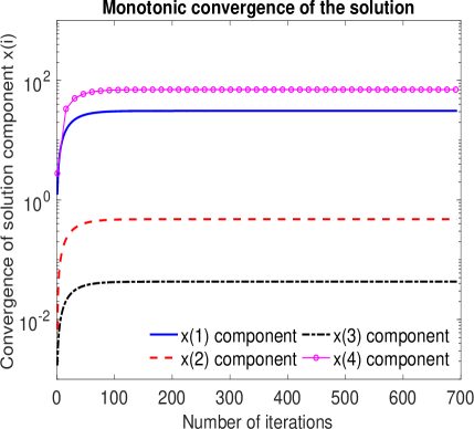
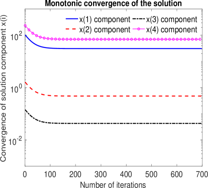
The monotonic convergence theorem proved in Section 4 is computationally established by solving the $4\times 4$ linear system (5.7) with multiple Right-Hand Side(RHS). The matrix and both the splittings satisfy all the required conditions mentioned in the theorem. Also, the initial approximations $x_{0}={[0,0,0,0]}^{T}$ and $y_{0}={[106.5647,10,1,241.9189]}^{T}$ satisfy the necessary conditions required by Theorem 4.1. Only the first column of the RHS matrix is used for the two-stage iteration method to generate Fig.1 corresponding to the iteration numbers. One can observe here, each component of the solution vector converges monotonically. In (a), the convergence is monotonically increasing. In (b), it is monotonically decreasing. And one can observe from the above figure that both are converging to single solution vector ${{\mathcal{A}}^{-1}}\mathcal{B}(:,1)$.

Next, our interest is to understand the computational aspect of the two-stage iterative method using the type-II splittings. Our matrix computations considered the $4\times 4$ transition matrix (5.1) of the pandemic model with standard iteration scheme (1.2) and two-stage iteration scheme (1.5), and similarly an extended $64\times 64$ matrix using the block matrix formulation (5.4) of (5.1). In two-stage Algorithm-1, we have used SOR type splitting with a relaxation parameter $\omega$. In Table-1, we have compared the standard iteration scheme with the two-stage standard iteration scheme corresponding to $\omega=1$ and $\omega=1.7$. The data listed in table shows that the two-stage iteration scheme for $\omega=1.7$ is faster than the standard iteration scheme and the two-stage iteration scheme with $\omega=1$.

When the condition numbers of the matrices become larger, the two-stage iteration scheme with $\omega=1.7$ converges gradually faster than the two-stage iteration scheme for $\omega=1$. The condition number is higher when the rate at which the recovered individuals are reinfected (or $\phi$ value) in the model is bigger, so we have considered the value of $\phi$ as 0.07, 0.08, 0.09 and 0.10, such that the condition number increase gradually and the iteration numbers also increase. In Table-1, we have computed condition number only for $4\times 4$ matrices as there is no significant change in condition number for $64\times 64$ size matrices when $\phi$ values are same. Similarly, we have computed the spectral radius only for $64\times 64$ size.

Table 1: Comparison between standard iteration scheme and two-stage iteration scheme
$\phi$Β -Β value One stage Two-stage($\omega$=1) Two-stage($\omega$=1.7)
Matrix size $4\times 4$ No. of iterations      $\kappa(\mathcal{A})~{}~{}~{}~{}~{}$
0.07 136 68 71 27.36
0.08 207 104 83 39.60
0.09 380 190 108 69.33
0.10 1428 714 149 $2.43\times{10}^{+02}$
Matrix size $64\times 64$ No. of iterations $\rho(T)$
0.07 142 71 72 0.686
0.08 218 109 89 0.733
0.09 400 200 116 0.778
0.10 1496 748 154 0.820

6 Acknowledgements

The second(NM) and last(DM) authors acknowledge the support provided by Science and Engineering Research Board, Department of Science and Technology, New Delhi, India, under the grant numbers MTR/2019/001366 and MTR/2017/000174, respectively. We would also like to thank the Government of India for introducing the work from home initiative during the COVID-19 pandemic.

References

  • [1] Bai, Z.-Z; Wang, D.-R., The monotone convergence of the two-stage iterative method for solving large sparse systems of linear equations, Appl. Math. Lett. 10 (1997), 113-117.
  • [2] Berman, A.; Plemmons, R. J., Cones and iterative methods for best least squares solutions of linear systems, SIAM J. Numer. Anal. 11 (1974), 145-154.
  • [3] Berman, A.; Plemmons, R. J., Non-negative matrices in the mathematical science, SIAM, Philadelphia, 1994.
  • [4] Cao, Z.-H., Rounding error analysis of two-stage iterative methods for large linear systems, Appl. Math. Comput. 139 (2003), 371-381.
  • [5] Climent, J.-J.; Perea, C., Comparison theorems for weak nonnegative splittings of $K$-monotone matrices, Electron. J. Linear Algebra 5 (1999), 24-38.
  • [6] Climent, J.-J.; Perea, C., Comparison theorems for weak splittings in respect to a proper cone of nonsingular matrices, Linear Algebra Appl. 302/303 (1999), 355-366.
  • [7] Climent, J.-J.; Perea, C., Some comparison theorems for weak non-negative splittings of bounded operators, Linear Algebra Appl. 275/276 (1998), 77-106.
  • [8] Diekmann, O.; Heesterbeek, J. A. P.; Metz, J. A .J, On the definition and the computation of the basic reproduction ratio, $R_{o}$ in models for infectious diseases in heterogeneous populations, J. Math. Biol. 28 (1990), 365-382.
  • [9] Frommer, A.; Szyld, B., H-splitting and two-stage iterative methods, Numer. Math. 63 (1992), 345-356.
  • [10] He, Q.; Wang, X.; Lei, Z.; Huang, M.; Cai, Y.; Ma, L., TIFIM: A Two-stage Iterative Framework for Influence Maximization in Social Networks, Appl. Math. Comput. 354 (2019), 338–352.
  • [11] Khajanchi, S.; Sarkar, K., Forecasting the daily and cumulative number of cases for the COVID-19 pandemic in India, Β (2020),Β https://arxiv.org/abs/2006.14575
  • [12] KochaΕ„czyk, M.; Grabowski, F.; Lipniacki, T., Accounting for super-spreading gives the basic reproduction number $R_{0}$ of COVID-19 that is higher than initially estimated, medRxiv 2020.04.26.20080788; DOI: 10.1101/2020.04.26.20080788
  • [13] Lewis, M. A.; Shuai, Z.; van den Driessche, P., A general theory for target reproduction numbers with applications to ecology and epidemiology, J. Math. Biol. 78 (2019), 2317–2339.
  • [14] Marek, I.; Szyld, D.B., Comparison theorems for weak splittings of bounded operators, Numer. Math 58 (1990), 389-397.
  • [15] MigallΓ³n, H.; MigallΓ³n, V.; PenadΓ©s, J., Alternating two-stage methods for consistent linear systems with applications to the parallel solution of Markov chains, Adv. Eng. Softw. 41 (2010), 13-21.
  • [16] MigallΓ³n, H.; MigallΓ³n, V.; PenadΓ©s, J., Parallel two-stage algorithms for solving the PageRank problem, Adv. Eng. Softw. 125 (2018), 188–199.
  • [17] Mishra, N.; Mishra, D., Two-stage iterations based on composite splittings for rectangular linear systems, Comput. Math. Appl. 75 (2018), 2746-2756.
  • [18] Nichols, N. K., On the convergence of two-stage iterative processes for solving linear equations, SIAM J. Numer. Anal. 3 (1973), 460-469.
  • [19] Ortega, J. M.; Rheinboldt, W. C., Monotone iterations for nonlinear equations with application to Gauss-Seidel methods, SIAM J. Numer. Anal. 4 (1967), 171-190.
  • [20] Prem, K.; Cook, A. R.; Jit, M., Projecting social contact matrices in 152 countries using contact surveys and demographic data, PLoS Comp. Bio, 13 (2017), e1005697.
  • [21] Singh, Rajesh; Adhikari, R., Age-structured impact of social distancing on the COVID-19 epidemic in India, (2020), arXiv preprint arXiv:2003.12055.
  • [22] Smith, J., The coupled equation approach to the numerical solution of the biharmonic equation by finite differences, SIAM J. Numer. Anal. 5 (1969), 323-339.
  • [23] van den Driessche, P.; Watmough, J., Further notes on the basic reproduction number, in Mathematical Epidemiology, F. Brauer, P. van den Driessche, and J. Wu, eds., Lecture Notes in Math. 1945, Springer, Berlin, (2008), 159-178.
  • [24] Varga, R. S., Matrix Iterative Analysis, Springer-Verlag, Berlin, 2000.
  • [25] Viceconte, G.; Petrosillo, N., COVID-19 R0: Magic number or conundrum?, Infect. Dis. Rep. 12 (2020), 8516-8517.
  • [26] Wachspress, E. L., Iterative solution of elliptic systems and applications to the neutron diffusion equations of reactor physics, Prentice-Hall, Englewood Cliffs, N.J., 1966.
  • [27] Wang, C, Comparison results for $K$-nonnegative double splittings of $K$-monotone matrices, Calcolo 54 (2017), 1293-1303.
  • [28] WoΕΊnicki, Z. I., Non-negative splitting theory, Japan J. Ind. Appl. Math. 11 (1994), 289-342.