Visualizing Classification Structure of Large-Scale Classifiers

Abstract

We propose a measure to compute class similarity in large-scale classification based on prediction scores. Such measure has not been formally proposed in the literature. We show how visualizing the class similarity matrix can reveal hierarchical structures and relationships that govern the classes. Through examples with various classifiers, we demonstrate how such structures can help in analyzing the classification behavior and in inferring potential corner cases. The source code for one example is available as a notebook at https://github.com/bilalsal/blocks.

1 Introduction

Classes that are highly similar are harder to separate from each other than from other classes. A variety of methods leverage this insight to improve multi-class classifiers (Amit et al., 2007; Deng et al., 2014; Murdock et al., 2016). The curators of ImageNet noted that visual object categories inherently follow a hierarchical similarity structure that is reflected in the confusion matrix of various ImageNet classifiers (Deng et al., 2010). Recent work demonstrates how this structure is further reflected in the features learned at successive layers in deep neural networks (Alsallakh et al., 2018a).

Inspired by the above-mentioned observations, our goal is to provide generic means to analyze and visualize class similarity structure in large-scale classification. Such analysis helps understand the features learned by a classifier to discriminate between classes. Confusion matrices fall short of enabling such analysis in a generic way. Our contributions include (1) a novel class similarity measure based on prediction scores, described in Section 2, and (2) means to visualize the class similarity matrix with examples of structures this matrix can reveal in three large-scale datasets, described in Section 3.

2 Rethinking Class Similarity

Both pieces of work mentioned in Section 1 rely on confusion matrices to analyze classification structure (Alsallakh et al., 2018a; Deng et al., 2010). When ordered according to the ImageNet synset hierarchy, this matrix captures the majority of confusions in few diagonal blocks that correspond to coarse similarity groups. Each of these blocks, in turn, can exhibit a nested block pattern that corresponds to narrower groups in the hierarchy. As we illustrate in Section 3, confusion matrices might fail to exhibit such pattern that reflects similarity structures due to the following reasons:

• Sparsity: Large confusion matrices usually contain more cells than labeled data, leaving the majority of cells empty, even with a relatively high error rate.

• Class imbalance: When reordering an imbalanced confusion matrix, the computed order is determined mainly by over-represented classes. This limits the possibilities to explore similarities involving under-represented classes, even if they constitute the majority.

• Multi-label classification: Confusion matrices are ill-defined in such problems. A multi-label classifier makes an error either by missing one label from the multi-labeled ground truth or by predicting a superfluous label. In both cases, the error cannot be attributed to a pair of classes as in a confusion matrix.

These characteristics are prevalent in large-scale classification as we exemplify with three popular datasets. The appendix provides two further examples.

The limited applicability of confusion matrices for similarity analysis is due to the reliance on pair-wise class confusions as a proxy of class similarity. If the classifier makes no errors, the matrix will be diagonal and hence will fail to show underlying class similarities. Moreover, when an error occurs, only the top-1 prediction of the classifier record the information. This discards the remaining top-k guesses of the classifier whose scores contain rich information about the result. Hinton et al. leverage these scores to distill essential knowledge about a classifier (Hinton et al., 2014), noting that they carry rich information about similarity structure in the data. We use these scores to analyze and visualize class similarities.

Similarity based on Prediction Scores

Given a set of $m$ classes $C=\{c_{j}:1\leq j\leq m\}$, we treat the scores $p_{i,j}$ computed by the classifier for each class $c_{j}$ as a random variable $P_{j}$ over the set of samples $X=\{x_{i}:1\leq i\leq n\}$. This enables us to formulate class similarity as correlation between these variables. Several measures of dependence between two variables have been defined. Pearson’s correlation coefficient measures the linear relationship between two random variables as follows:

$$\rho_{j_{1},j_{2}}=\frac{E(P_{j_{1}}\cdot P_{j_{2}})-E(P_{j_{1}})\cdot E(P_{j_{2}})}{\sqrt{{E(P_{j_{1}}}^{2})-E(P_{j_{1}})^{2}}\cdot\sqrt{{E(P_{j_{2}}}^{2})-E(P_{j_{2}})^{2}}}$$ (1)

where $E$ denotes the expected value and is computed as the mean over all $x_{i}\in X$. The expected value $E(P_{j_{1}}\cdot P_{j_{2}})$ is high when $c_{j_{1}}$ and $c_{j_{2}}$ frequently appear together among the top guesses, which supports their overall similarity. It is worth mentioning that we do not use the computed correlations to perform statistical significance test. Instead, we use these correlations to define a class similarity matrix $M$ that has several advantages over a confusion matrix:

• A prediction does not need to be erroneous for a sample to contribute to the similarity computation, alleviating the sparsity problem of the computed matrix.

• No ground-truth labels are required, as evident in Eq. 1. This enables computing class similarity over unlabeled datasets as long as a prototypical classifier is available.

• The coefficient can be naturally applied to multi-labeled datasets because they do not rely on comparing ground truth with predictions.

• The coefficient is symmetric with respect to the classes and is normalized with respect to their frequencies. Both properties are crucial to visualize possible block patterns in $M$ and to handle class imbalance.

Statistical Analysis of the Similarity Measure

It is important to pay attention to the distribution of the similarity values. As we demonstrate in Section 3, a nearly-normal distribution of the values in $M$ enables both small and large similarity groups to emerge when visualizing M. For illustration, we examine this condition on the Places365 dataset (Zhou et al., 2017). This dataset contains 365 classes that represent scenes and places. We use a pre-trained AlexNet classifier provided by the dataset curators to compute prediction scores and model activations for all 36500 samples in the validation set.

The output of classifiers is usually normalized into probabilities, with $1/m$ being the average probability, where $m$ denotes the number of classes. This makes the distribution of $P_{j}$ drastically skewed to the right. Figure 1a-left depicts this distribution for a random class in Places365. Figure 1a-right depicts the distribution if the similarity values in $M$, computed for all pairs of classes in the dataset. This distribution drastically skewed to the right, which can mask global classification structure when visualizing $M$ as only small coherent clusters can emerge from the relatively few matrix cells corresponding to the long tail. We examined two solutions to this problem:

• Using raw prediction scores (logits): Figure 1b-left depicts the distribution of these logits for a random class in Places365. When used as random variables in Eq. 1, the logits result in a less skewed distribution of similarity values, compared with probabilities, as illustrated in Figure 1b-right. Logits are often used to circumvent similar problems (Bucilua et al., 2006; Shrikumar et al., 2017).

• Using Spearman’s rank coefficient: This is equivalent to Pearson’s coefficient applied to the rank values instead of the actual scores. The distribution of the ranks over the range $[1,m]$ is more uniform (Figure 1c-left) compared with probabilities, leading to near-normal distribution of the similarity values as illustrated in Figure 1c-right.

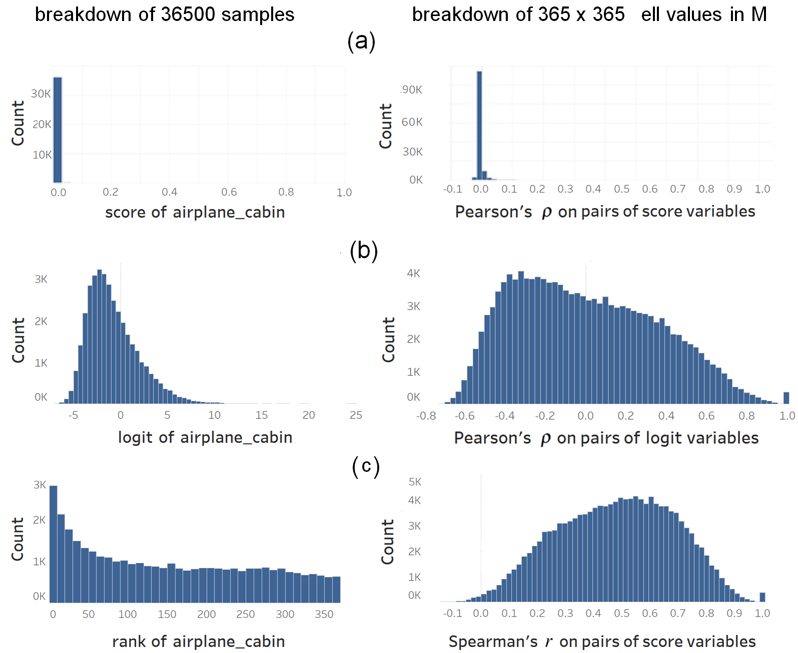
Figure 1: The distribution of different types of input values (left) and of the corresponding score-based similarities (right) computed using: (a) Pearson’s coefficient applied to probabilities, (b) Pearson’s coefficient applied to logits, and (c), Spearman’s rank coefficient applied to probabilities.

The use of logits preserves fine-grained differences in the scores, whereas the use of ranks results in more rough similarity structures. We recommend considering both options as we discuss in Section 4.

Figure 2: (a) The logit-based similarity matrix between the classes of Places365, ordered using hclust. The matrix exhibits two major groups of scene categories, indoor and outdoor environments. (b) The same matrix ordered according to the predefined taxonomy.

3 Visualizing Class Similarity

A 2D heatmap offers a natural way to visualize the similarity matrix $M$. A key factor impacting the visualization is the ordering of the rows and columns. Behrisch et al. surveyed seriation algorithms (Behrisch et al., 2016) illustrating the patterns they can expose in large matrices. Our goal is to find a hierarchical structure over the classes. Among available algorithms in $R$, we found that hclust can consistently reveal block patterns in various datasets if the values in the matrix follow a nearly-normal distribution. We use complete linkage, the default agglomeration method in hclust.

Figure 2a depicts the logit-based similarity matrix between 365 classes of Places365 described in Section 2. The hclust algorithm succeeds in revealing two major blocks along the diagonal, corresponding to rooms and outdoor scenes respectively. In fact, the curator of the dataset selected their scene categories from a two-level scene taxonomy, depicted in Figure 2b. Parallel to our findings, this taxonomy divides the scenes into indoor and outdoor groups, with the later group further divided into man-made and natural outdoor scenes. Ordering the matrix according to this taxonomy results in dense diagonal sub-blocks that correspond to its second level. These sub-blocks largely correspond to the fine-grained ones found by hclust.

3.1 Recovering Hierarchical Relations Among Classes

In multi-label datasets, the classes can vary in their level of abstraction, often leading to overlapping semantics. This aims to maximize the prediction usefulness: The classifier can still predict correct high-level classes in case it fails to predict fine-grained ones. An example of such dataset is AudioSet (Gemmeke et al., 2017). This dataset contains about 2 million audio clips, each assigned one or more labels from 527 categories that follow a predefined sound taxonomy. Among the classes, 408 represent fine-grained categories such as Steel guitar, while 119 are at multiple levels of abstraction such as Guitar, Musical Instrument, and Music. AudioSet has a high degree of class imbalance as we demonstrate in Figure 3.

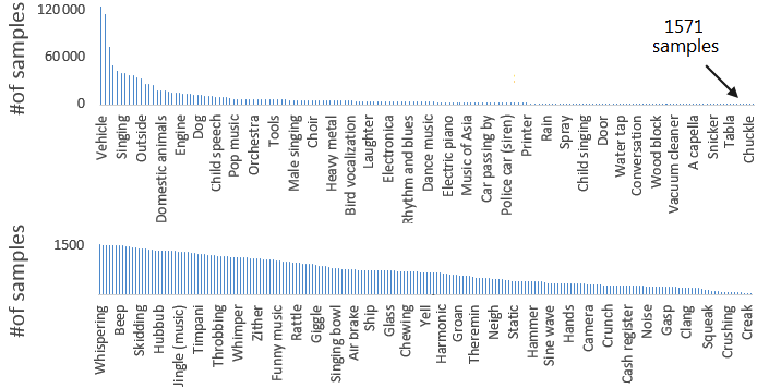
Figure 3: The frequency of 527 classes in AudioSet, excluding Music and Speech, each appearing as labels in nearly 1 million samples. For better readability we print textual labels for a few classes only and split the long tail of the distribution.

Figure 4a depicts the predefined taxonomy of the classes, along with their co-occurrence matrix in the multi-labeled ground truth. The matrix suggests high co-occurrence within the Music group, with other broad taxonomy groups being far less coherent. The matrix further exhibits star patterns (Behrisch et al., 2016) in form of salient line crossings. We mark the corresponding classes with a tick mark on the right side of the matrix.

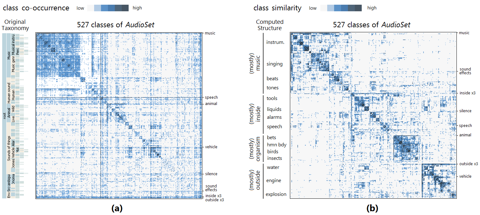
Figure 4: The classification structure in AudioSet based on (a) the co-occurrence matrix of the multi-labeled ground truth, ordered according to a predefined sound taxonomy, and (b) the logit-based similarity matrix, ordered using hclust. It reveals more coherent groups among the classes than the ones in (a) and surfaces high-level classes such as Inside and Outside that encompass other classes.

The lines indicate that these classes exhibit high co-occurrence with a variety of other classes. The lines stand out most for Music and Speech, each appearing in about $49\%$ of the samples. The lines are also visible for Vehicle, and Animal, each also having multiple subclasses in the taxonomy. Finally, a few subclasses of Inside and Outside form a dense band, visible in the bottom or right side of the matrix. These subclasses serve as meta descriptors of sound events, leading to frequent co-occurrence with other classes. The matrix falls short of exposing further structures due to its high susceptibility to class imbalance.

Figure 4b depicts the logit-based similarity matrix of the same dataset, with scores computed using VGGish (Hershey et al., 2017). This matrix reveals several coherent and semantically-related groups among the classes that were masked in the co-occurrence matrix. Furthermore, the matrix reveals flame patterns (Lekschas et al., 2018) around major blocks along the diagonal. These flames correspond to star patterns in the co-occurrence matrix, however, defining more accurate and informative spans over the classes. We annotate the four major spans along the left side of the matrix. The Music and Animal classes span two blocks that contains most of their subclasses in the original taxonomy, in addition to other semantically related classes that were under Sound of things and Human. Interestingly, two new major blocks emerge that were marginalized in the original taxonomy, Inside and Outside. The corresponding classes are grouped under Acoustic environment in the original taxonomy. This suggests that whether the sound event takes place in indoor or outdoor environments plays a major role in the predictions made by the classifier.

3.2 Recovering Split and Failed Similarity Groups

In many classification problems, overlapping class similarity groups might exist that do not fit in a strict hierarchy. This happens, for example, with the VGGFace dataset whose classes represent 2,622 celebrities (Parkhi et al., 2015). Figure 5 shows the logit-based similarity matrix computed over a balanced subset of 100 images per celebrity using the reference classifier provided by the dataset curators. Ordering the matrix using hclust divides the classes into two broad similarity groups: male celebrities and female celebrities. Within each group, the algorithm finds subgroups based on skin color, hair color, medium color (monochrome vs. multichrome), wrinkles, and other facial features. These data features potentially define coherent similarity groups. However, these groups are split as hclust identifies gender as the top level of the hierarchy. In fact, the classifier rarely confuses celebrities of different gender for each other. By looking at cases with such confusion, we found it often occurs with images scrapped for certain celebrities that did contain their opposite-sex spouses and went unnoticed when curating VGGFace.

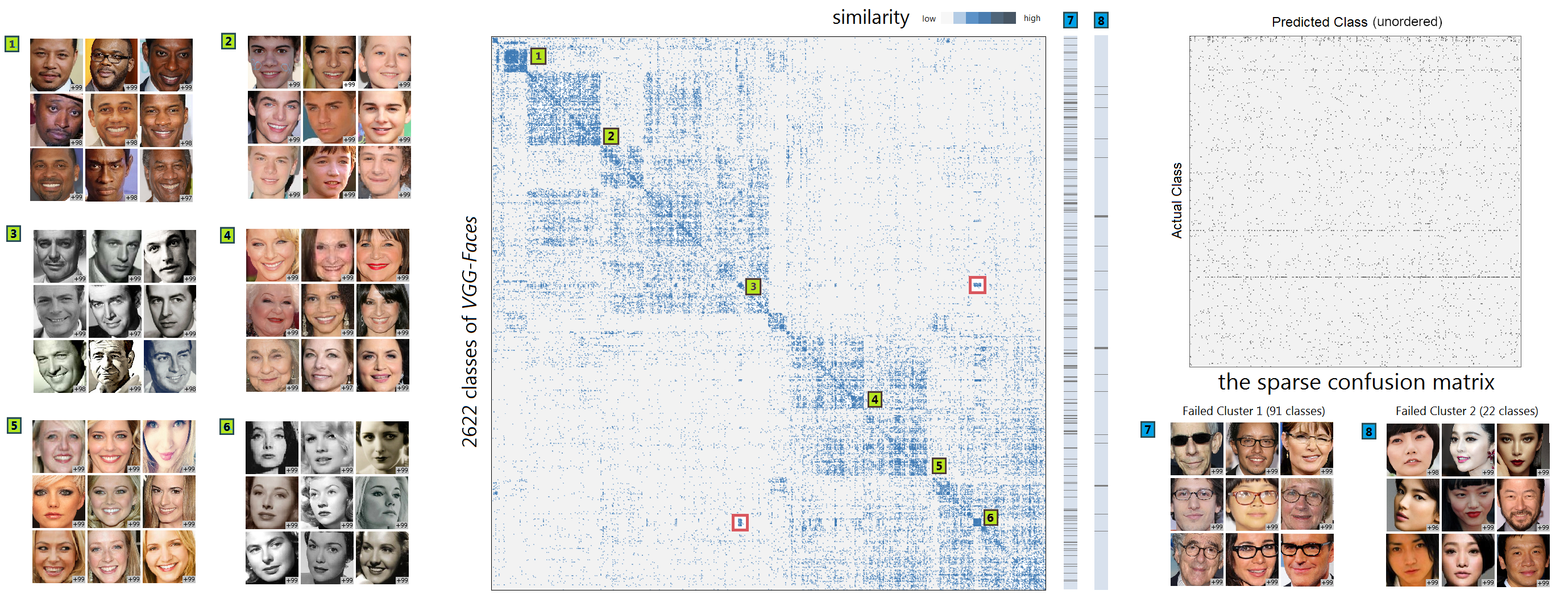
Figure 5: The logit-based similarity matrix between the classes of VGGFace, which contains images of 2622 celebrities. We annotate selected fine-grained clusters in green and show examples of the corresponding classes. These clusters do not surface in the confusion matrix. Two failed clusters are annotated in blue, along with corresponding columns that show their dispersion in the matrix.

Two dense off-diagonal clusters in the matrix are annotated with red boxes in Figure 5. These clusters indicate high similarity between two subgroups of different gender that correspond to actors whose images are predominantly monochrome. We refer to such related subsets as a split group. Dense off-diagonal sub-clusters are useful to identify split groups, however, they might not always emerge. For example classes that represent celebrities who usually wear glasses turn out to have high similarity to each other. Nevertheless, hclust disperses these classes across different subgroups in the matrix, as illustrated in an auxiliary column in Figure 5. We refer to such groups as failed groups.

Failing to consolidate potentially coherent groups is an inherent issue in hierarchical clustering, as it only allows inclusion and exclusion relations between the groups. One solution to recover failed groups is to apply fuzzy clustering on the classes, with the rows of the similarity matrix $M$ serving as feature vectors. This clustering paradigm can extract overlapping groups over the classes. Figure 5 depicts two recovered groups in VGGFace annotated as (7) and (8): glass wearers and celebrities of Asian ethnicity. These groups suggest that the classifier develops corresponding facial features and relies on them to recognize the celebrities. Such insights are very useful to infer potential corner cases of the classification model as we discuss in Section 5.

4 Comparison with Related Work

Class similarity measures have been proposed for various purposes. They have traditionally been based on raw input features (Roth et al., 2003), derived features (Opelt et al., 2006), or multi-labeled ground truth (Cissé et al., 2016; Wu et al., 2015). Recent work has utilized learned features with cosine similarity (Ye & Guo, 2017; Hohman et al., 2019). Nevertheless, little attention has been paid to visualizing the similarity matrix and analyzing the classification structure. Likewise, prediction scores have been utilized to analyze classifiers, focusing however on their distribution (Katehara et al., 2017), or calibration (Guo et al., 2017). The advantage of scores is that they reflect what the classifier deems similar, offering a window to analyze its behaviour. 2D projections of the data space have been utilized to assess class separability (Iwata et al., 2005) and to reveal structures such as ones dictated by visual (Nguyen et al., 2016) or linguistic features (Reif et al., 2019). Unlike matrices, scatter plots fall short of providing a scalable overview of hierarchical structures.

Matrices have been extensively used to analyze correlations (Bautista et al., 2016) or distances (Brasselet et al., 2009) at the sample level, or at the layer level (Gigante et al., 2019; Li et al., 2016; Raghu et al., 2017). We did not find prior work on utilizing matrices for class similarity, other than confusion matrices. As discussed in Section 2, our measure is more generic than confusion matrices: In all of our examples, confusion matrices are either undefined (Section 3.1), sparse (Figure 5-right), or fail to reveal coarse groups as we demonstrate in the provided notebook.

5 Applicability and Future Work

Understanding structure can inform additional supervision to regularize neural classifiers (Alsallakh et al., 2018b). An earlier work demonstrates how a confusion matrix enables spotting subtle data-quality issues, as they pop out as outliers off the diagonal blocks (Alsallakh et al., 2018a). This type of analysis enabled us to find various quality issues in VGGFace such as duplicate identities, hardly distinguishable twins, and mistaking celebrities for their spouses. Furthermore, based on the similarity groups we found in that dataset (Figure 5), we identified potential dependence of certain classes on specific image features such as monochrome input or eye glasses. We curated external images of the corresponding celebrities that did not have the respective features, for example, face images without eye glasses of celebrities in group (7). The prediction scores for these images dropped significantly, leading to frequent misclassification. Finally, the structure enables comparing the established groups w.r.t. robustness to perturbations or to adversarial attacks.

Matrices can reveal coarse similarity groups between thousands of classes, especially when equipped with cut-off sliders and other visual boosting techniques (Oelke et al., 2011). On the other hand, computing and reordering large matrices can be resource intensive, however, within feasible limits: about 2GB of memory and a few minutes of compute on an average CPU suffice for the examples we presented. Nevertheless, matrix seriation remains an open challenge as multiple orderings are plausible. While we recommend hclust for an initial overview, we encourage exploring different linkage methods, ordering algorithms, and correlation coefficients, examining the distribution of computed similarities, and employing further algorithms to extract potentially failed groups.

Our future work aims to provide interactive means to ease examining alternative ordering and failed groups. We also aim to apply our approach to extreme and few-shot classification in order to analyze the behavior of classifiers designed to address long-tail distributions (Chen et al., 2019; Wang et al., 2017). Thanks to its ability to handle class imbalance, our approach can help in analyzing how classes with few shots are affiliated with more common classes. Finally, our approach can help understand the evolution of classification structure over multiple layers in neural classifiers.

6 Conclusion

We presented means to compute and analyze class similarities in large-scale classification based on prediction scores. Our means can handle datasets involving class imbalance, multi-labeled samples, as well as datasets with few prediction errors or scarce labels. We provided extensive means to visualize the class similarity matrix and illustrated with four datasets how it can expose various types of relationships between the classes. Our analytical and visual means inform the analysis of class similarities in a way that has not been formally addressed in the literature.

Appendix

Here we present two further examples on visualizing classification structure.

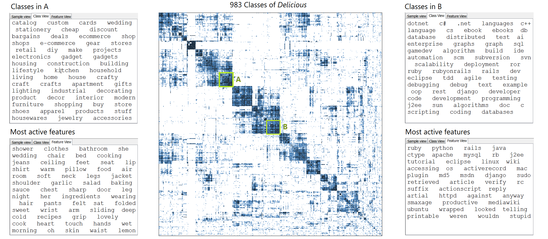
Figure 6: The probability-based similarity matrix of the Delicious text classification dataset (Tsoumakas et al., 2008). The scores are computed using FastXML (Prabhu & Varma, 2014) and the similarities are computed using Spearman’s rank coefficient. Two groups of classes are highlighted whose labels are listed in the respective text boxes. Group A contains predominantly shopping-related tags, while group B captures programming-related tags.

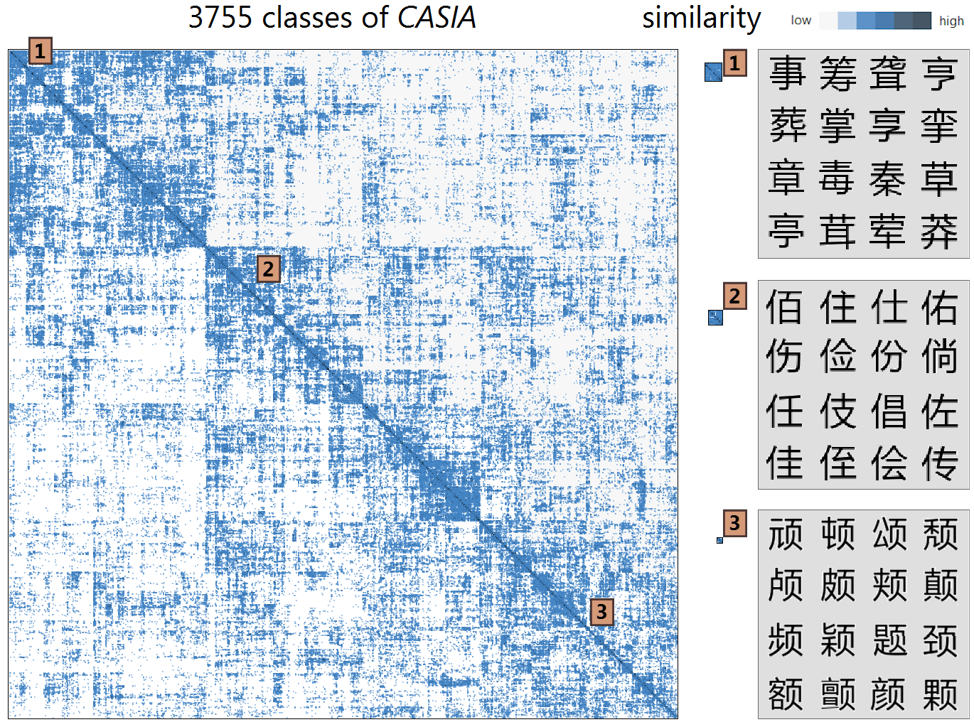
Figure 7: logit-based similarity matrix between 3,755 Chinese characters from the CASIA validation dataset (Liu et al., 2011). The dataset contains 60 samples per Chinese characters which we classify using Chinese offline handwriting classifier (Wang, 2017) trained on the CASIA training set. The matrix reveals a few coarse groups, each containing a variety of coherent fine-grained groups along the diagonal, three of which are annotated along with examples of their classes (depicted with a typeface). The character classes in the fine-grained groups share highly similar or identical strokes, e.g., a horizontal line in the top (1) or a shared stroke on the left (2) or right side (3).

References

- Alsallakh et al. (2018a) Alsallakh, B., Jourabloo, A., Ye, M., Liu, X., and Ren, L. Do convolutional neural networks learn class hierarchy? IEEE Transactions on Visualization and Computer Graphics, 24(1), 2018a.
- Alsallakh et al. (2018b) Alsallakh, B., Jourabloo, A., Ye, M., Liu, X., and Ren, L. Understanding the error structure as a key to regularize convolutional neural networks. In Conference on Machine Learning and Systems, 2018b.
- Amit et al. (2007) Amit, Y., Fink, M., Srebro, N., and Ullman, S. Uncovering shared structures in multiclass classification. In International Conference on Machine Learning (ICML), pp. 17–24, 2007.
- Bautista et al. (2016) Bautista, M. A., Sanakoyeu, A., Tikhoncheva, E., and Ommer, B. CliqueCNN: Deep unsupervised exemplar learning. In Advances in Neural Information Processing Systems (NeurIPS), pp. 3846–3854, 2016.
- Behrisch et al. (2016) Behrisch, M., Bach, B., Henry Riche, N., Schreck, T., and Fekete, J.-D. Matrix reordering methods for table and network visualization. Computer Graphics Forum, 35(3):693–716, 2016.
- Brasselet et al. (2009) Brasselet, R., Johansson, R., and Arleo, A. Optimal context separation of spiking haptic signals by second-order somatosensory neurons. In Advances in Neural Information Processing Systems (NeurIPS), pp. 180–188, 2009.
- Bucilua et al. (2006) Bucilua, C., Caruana, R., and Niculescu-Mizil, A. Model compression. In ACM International Conference on Knowledge discovery and data mining (KDD), pp. 535–541, 2006.
- Chen et al. (2019) Chen, W.-Y., Liu, Y.-C., Kira, Z., Wang, Y.-C. F., and Huang, J.-B. A closer look at few-shot classification. In International Conference on Learning Representations, 2019.
- Cissé et al. (2016) Cissé, M., Al-Shedivat, M., and Bengio, S. Adios: Architectures deep in output space. In International Conference on Machine Learning (ICML), pp. 2770–2779, 2016.
- Deng et al. (2010) Deng, J., Berg, A. C., Li, K., and Fei-Fei, L. What does classifying more than 10,000 image categories tell us? In European Conference on Computer Vision (ECCV), pp. 71–84. Springer, 2010.
- Deng et al. (2014) Deng, J., Ding, N., Jia, Y., Frome, A., Murphy, K., Bengio, S., Li, Y., Neven, H., and Adam, H. Large-scale object classification using label relation graphs. In European Conference on Computer Vision (ECCV), pp. 48–64. Springer, 2014.
- Gemmeke et al. (2017) Gemmeke, J. F., Ellis, D. P., Freedman, D., Jansen, A., Lawrence, W., Moore, R. C., Plakal, M., and Ritter, M. Audio set: An ontology and human-labeled dataset for audio events. In International Conference on Acoustics, Speech and Signal Processing, pp. 776–780, 2017.
- Gigante et al. (2019) Gigante, S., Charles, A. S., Krishnaswamy, S., and Mishne, G. Visualizing the phate of neural networks. In Advances in Neural Information Processing Systems (NeurIPS), pp. 1840–1851, 2019.
- Guo et al. (2017) Guo, C., Pleiss, G., Sun, Y., and Weinberger, K. Q. On calibration of modern neural networks. In International Conference on Machine Learning, pp. 1321–1330, 2017.
- Hershey et al. (2017) Hershey, S., Chaudhuri, S., Ellis, D. P., Gemmeke, J. F., Jansen, A., et al. Cnn architectures for large-scale audio classification. In International Conference on Acoustics, Speech and Signal Processing, pp. 131–135, 2017.
- Hinton et al. (2014) Hinton, G., Vinyals, O., and Dean, J. Distilling the knowledge in a neural network. In NeurIPS Workshop on Deep Learning and Representation Learning, 2014.
- Hohman et al. (2019) Hohman, F., Park, H., Robinson, C., and Chau, D. H. P. Summit: Scaling deep learning interpretability by visualizing activation and attribution summarizations. IEEE Transactions on Visualization and Computer Graphics, 26(1):1096–1106, 2019.
- Iwata et al. (2005) Iwata, T., Saito, K., Ueda, N., Stromsten, S., Griffiths, T. L., and Tenenbaum, J. B. Parametric embedding for class visualization. In Advances in Neural Information Processing Systems (NeurIPS), pp. 617–624, 2005.
- Katehara et al. (2017) Katehara, M., Beauxis-Aussalet, E., and Alsallakh, B. Prediction scores as a window into classifier behavior. In NeurIPS Symposium on Interpretable Machine Learning, 2017.
- Lekschas et al. (2018) Lekschas, F., Bach, B., Kerpedjiev, P., Gehlenborg, N., and Pfister, H. HiPiler: Visual exploration of large genome interaction matrices with interactive small multiples. IEEE Transactions on Visualization and Computer Graphics, 24(1):522–531, 2018.
- Li et al. (2016) Li, Y., Yosinski, J., Clune, J., Lipson, H., and Hopcroft, J. E. Convergent learning: Do different neural networks learn the same representations? In International Conference on Learning Representations (ICLR), pp. 196–212, 2016.
- Liu et al. (2011) Liu, C.-L., Yin, F., Wang, D.-H., and Wang, Q.-F. Casia online and offline chinese handwriting databases. In International Conference on Document Analysis and Recognition (ICDAR), pp. 37–41. IEEE, 2011.
- Murdock et al. (2016) Murdock, C., Li, Z., Zhou, H., and Duerig, T. Blockout: Dynamic model selection for hierarchical deep networks. In IEEE Computer Society Conference on Computer Vision and Pattern Recognition (CVPR), pp. 2583–2591, 2016.
- Nguyen et al. (2016) Nguyen, A., Yosinski, J., and Clune, J. Multifaceted feature visualization: Uncovering the different types of features learned by each neuron in deep neural networks. In ICML Workshop on Visualization for Deep Learning, 2016.
- Oelke et al. (2011) Oelke, D., Janetzko, H., Simon, S., Neuhaus, K., and Keim, D. A. Visual boosting in pixel-based visualizations. Computer Graphics Forum, 30(3):871–880, 2011.
- Opelt et al. (2006) Opelt, A., Pinz, A., and Zisserman, A. Incremental learning of object detectors using a visual shape alphabet. In IEEE Conference on Computer Vision and Pattern Recognition (CVPR), volume 1, pp. 3–10. IEEE, 2006.
- Parkhi et al. (2015) Parkhi, O. M., Vedaldi, A., and Zisserman, A. Deep face recognition. In British Machine Vision Conference, 2015.
- Prabhu & Varma (2014) Prabhu, Y. and Varma, M. Fastxml: A fast, accurate and stable tree-classifier for extreme multi-label learning. In ACM conference on Knowledge Discovery and Data Mining (SIGKDD), pp. 263–272. ACM, 2014.
- Raghu et al. (2017) Raghu, M., Gilmer, J., Yosinski, J., and Sohl-Dickstein, J. SVCCA: Singular vector canonical correlation analysis for deep learning dynamics and interpretability. In Advances in Neural Information Processing Systems (NeurIPS), pp. 6078–6087, 2017.
- Reif et al. (2019) Reif, E., Yuan, A., Wattenberg, M., Viegas, F. B., Coenen, A., Pearce, A., and Kim, B. Visualizing and measuring the geometry of bert. In Advances in Neural Information Processing Systems (NeurIPS, pp. 8592–8600, 2019.
- Roth et al. (2003) Roth, V., Laub, J., Müller, K.-R., and Buhmann, J. M. Going metric: Denoising pairwise data. In Advances in Neural Information Processing Systems, pp. 841–848, 2003.
- Shrikumar et al. (2017) Shrikumar, A., Greenside, P., and Kundaje, A. Learning important features through propagating activation differences. In International Conference on Machine Learning (ICML), pp. 3145–3153. JMLR. org, 2017.
- Tsoumakas et al. (2008) Tsoumakas, G., Katakis, I., and Vlahavas, I. Effective and efficient multilabel classification in domains with large number of labels. In ECML/PKDD Workshop on Mining Multidimensional Data, volume 21, pp. 53–59. sn, 2008.
- Wang (2017) Wang, T. CNN handwritten chinese recognition, 2017. Online: https://github.com/taosir/cnn_handwritten_chinese_recognition.
- Wang et al. (2017) Wang, Y.-X., Ramanan, D., and Hebert, M. Learning to model the tail. In Advances in Neural Information Processing Systems (NeurIPS), pp. 7029–7039, 2017.
- Wu et al. (2015) Wu, B., Lyu, S., Hu, B.-G., and Ji, Q. Multi-label learning with missing labels for image annotation and facial action unit recognition. Pattern Recognition, 48(7):2279–2289, 2015.
- Ye & Guo (2017) Ye, M. and Guo, Y. Zero-shot classification with discriminative semantic representation learning. In IEEE Conferenceon Computer Vision and Pattern Recognition (CVPR), pp. 7140–7148, 2017.
- Zhou et al. (2017) Zhou, B., Lapedriza, A., Khosla, A., Oliva, A., and Torralba, A. Places: A 10 million image database for scene recognition. IEEE Transactions on Pattern Analysis and Machine Intelligence, 2017.