The Atacama Cosmology Telescope: DR5 maps of 18 000 square degrees of the microwave sky from ACT 2008-2018 data

Abstract

This paper presents a maximum-likelihood algorithm for combining sky maps with disparate sky coverage, angular resolution and spatially varying anisotropic noise into a single map of the sky. We use this to merge hundreds of individual maps covering the 2008–2018 ACT observing seasons, resulting in by far the deepest ACT maps released so far. We also combine the maps with the full Planck maps, resulting in maps that have the best features of both Planck and ACT: Planck’s nearly white noise on intermediate and large angular scales and ACT’s high-resolution and sensitivity on small angular scales. The maps cover over 18 000 square degrees, nearly half the full sky, at 100, 150 and 220 GHz. They reveal 4 000 optically-confirmed clusters through the Sunyaev Zel’dovich effect (SZ) and 18 500 point source candidates at $>5\sigma$, the largest single collection of SZ clusters and millimeter wave sources to date. The multi-frequency maps provide millimeter images of nearby galaxies and individual Milky Way nebulae, and even clear detections of several nearby stars. Other anticipated uses of these maps include, for example, thermal SZ and kinematic SZ cluster stacking, CMB cluster lensing and galactic dust science. The method itself has negligible bias. However, due to the preliminary nature of some of the component data sets, we caution that these maps should not be used for precision cosmological analysis. The maps are part of ACT DR5, and are available on LAMBDA at https://lambda.gsfc.nasa.gov/product/act/actpol_prod_table.cfm. There is also a web atlas at https://phy-act1.princeton.edu/public/snaess/actpol/dr5/atlas.

1 Introduction

	Planck	ACT+Planck	ACT
f090
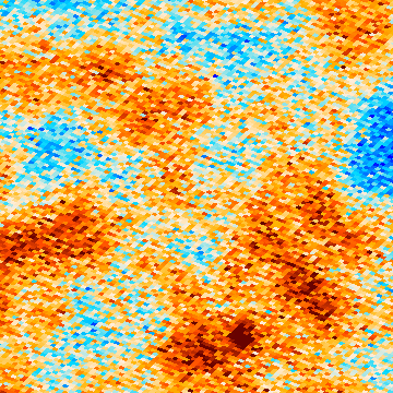
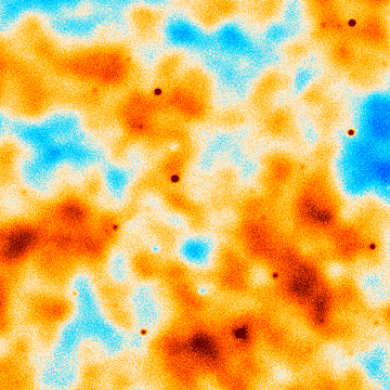
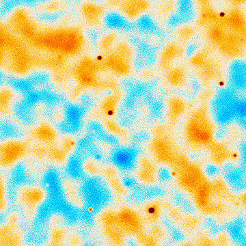
f150
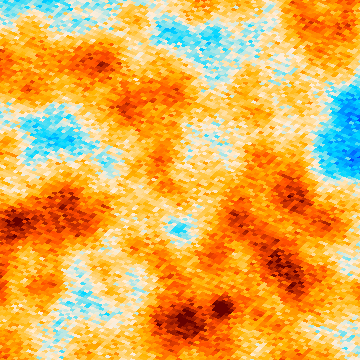
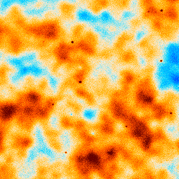
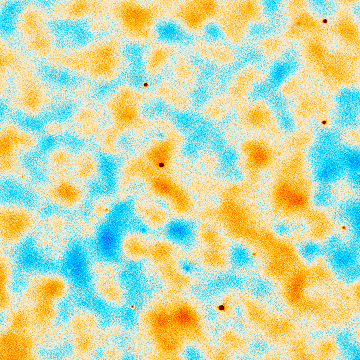
f220

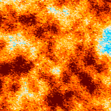
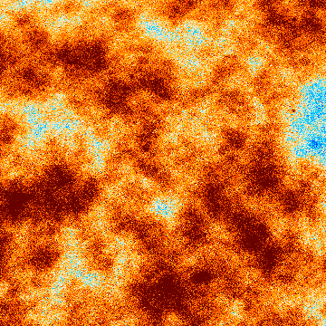
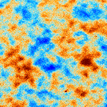
Figure 1: Comparison of Planck, ACT+Planck and ACT-only in a $3^{\circ}\times 3^{\circ}$ patch centered on RA = 231.5^∘, dec = 16.5^∘. The map of this region includes ACT daytime data. The ACT map depths in this region are 8/8/30 µK-arcmin at f090/f150/f220 (see figure 2 for band definitions). ACT+Planck is a substantial improvement over Planck alone, both in resolution and depth, and captures the larger scales that ACT alone has trouble measuring. See figure 22 for an image filtered to emphasize the point sources, clusters and other small-scale features.

Over the past three decades, cosmologists have been mapping the microwave sky with increasing precision. COBE (Bennett et al., 1994), WMAP (Bennett et al., 2003, 2013) and Planck (Planck Collaboration, 2013, 2018) have produced multi-frequency maps with nearly white (spatially uncorrelated) noise and with increasing angular resolution. These observations from space are complemented by measurements with ground based telescopes that have higher sensitivity and potentially higher resolution (e.g. SPT (Benson et al., 2014) and ACT (Thornton et al., 2016)), but suffer from large atmospheric noise contamination with complicated covariances at large scales.

This paper presents an approach to building tiled coadds of these heterogeneous maps. Section §2 describes the Planck and ACT data used in constructing the heterogeneous temperature and polarization maps used in the tiled coadding process. In this analysis, we use a larger set of the ACT data than used in Aiola et al. (2020) and Choi et al. (2020), including data from the 2017 and 2018 seasons as well as data from daytime observations. Section §3 describes the algorithms for coadding maps. While this paper describes applying these algorithms to the ACT and Planck data, our approach of producing tiled coadds of heterogeneous maps can be generalized to other data sets with complex noise properties.

Section §4 introduces the tiled constant correlation noise model used to approximate the noise properties of the maps. Section §5 describes how individual tiled coadded maps are calculated and then assembled into a full map. Section §6 describes the properties of the coadded maps. Section §7 reveals the maps and focuses on images of the astronomical objects revealed by the maps, and concludes by noting the maps’ limitations.

Previous related work includes, for example, Crawford et al. (2016) and Chown et al. (2018) (SPT+Planck); and Aghanim et al. (2019) and Madhavacheril et al. (2019) (ACT+Planck). The methods in this paper differ in that a) we model the spatial dependence and stripiness of the noise; b) we preserve the full resolution of the input maps; and c) we apply them to maps covering seven times the sky area.

The main product of this paper is a set of coadded maps. Figure 1 shows a small piece of the maps and provides a taste of the full data product. The figure compares Planck to the ACT+Planck and ACT-only coadds in total intensity in a $3^{\circ}\times 3^{\circ}$ sub-patch, showing both the much greater depth and resolution ACT provides and the large-scale information Planck adds. Only one of the $\sim 20$ point sources (red dots) we see in ACT panels can be seen in Planck, and none of the clusters (blue dots, three visible without filtering).

For each of the frequency bands f090, f150 and f220, centered at roughly 98 GHz, 150 GHz and 224 GHz (but see figure 2), we provide all combinations of ACT-only and ACT+Planck; day+night and night-only; and normal and source-free maps, each of which is a (43200,10320,3) FITS image containing Stokes parameters I, Q and U in single precision, for a total of 5.0 GB each (see appendix A). We also provide Planck maps reprojected to the same pixelization, as well as inverse white noise variance maps.

The full FITS images are available at https://lambda.gsfc.nasa.gov/product/act/actpol_prod_table.cfm (“DR5 2008-2018 Coadd maps”). A browser-based pannable, zoomable visualization of the maps can be found at https://phy-act1.princeton.edu/public/snaess/actpol/dr5/atlas.

2 The data

The combined sky maps presented in this article build on the data described in this section. In total, we have 78 data sets – sets of maps covering the same area with the same beam and noise properties, but made from independent splits (subsets) of the data; e.g. half-mission maps in the case of Planck. The splits in each data set are used to build the noise model in section 3.2. In total we have 276 such split maps, taking up a combined 260 GB for the signal maps and 136 GB for the corresponding inverse variance maps, which are estimates of the level of uncorrelated noise in each pixel. With the exception of the unpolarized ACT-MBAC data (see section 2.2), each map consists of three fields, one for each of the Stokes parameters, I (here called T), Q and U, for a total of 748 individual fields. The data sets are tabulated in table 1 and further described below.

These data sets fall into two categories: 1. Mature maps that are already properly calibrated. This includes the Planckmaps, the old ACT MBAC maps, and the ACT DR4 maps. The calibration of these products is described in their corresponding papers. 2. Preliminary maps, i.e. “Prelimnary Advanced ACTPol” and “Preliminary ACT daytime data”. These did not have mature calibration and so some work had to be done to calibrate them. This procedure is described in sections 2.2.3 and 2.2.4 (see also figure 3).

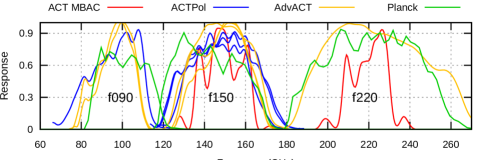
Figure 2: Comparison of the ACT and Planck bandpasses in the range 60 GHz to 270 GHz. (See Section 2.2 for description of the three ACT cameras: MBAC, ACTPol and Advanced ACTPol.) They fall into three groups, centered at roughly 90 GHz, 150 GHz and 220 GHz. We label these bandpass-groups f090, f150 and f220. In this paper we approximate all bandpasses in each group as being equivalent. This results in a small scale-dependence of the effective band center for non-CMB parts of the combined maps – see section 6.2.

Table 1: Data descriptions

Survey	Patch	RA (∘)		dec (∘)		Datasets 1	nsplit 2	total 3
Planck	Planck	0  –	360	-90  –	90	Planck f090+f150+f220	2	6
ACT-MBAC	South	-114  –	147	-57  –	-48	AR1+AR2 2008–2010	4	24
ACT-MBAC	Equ	-250  –	65	-2.4  –	2.6	AR1+AR2 2009–2010	4	16
ACT DR4	D1	140  –	161	-5  –	6	PA1 2013	4	4
ACT DR4	D5	-19  –	13	-7  –	6	PA1 2013	4	4
ACT DR4	D6	19  –	48	-11  –	1	PA1 2013	4	4
ACT DR4	D56	-23  –	54	-10  –	7	PA1+PA2 2014–2015, PA3 2015	4	24
ACT DR4	D8	-12  –	18	-52  –	-32	PA1+PA2+PA3 2015	4	16
ACT DR4	BN	102  –	257	-7  –	22	PA1+PA2+PA3 2015	4	16
ACT DR4	AA	0  –	360	-62  –	22	PA2+PA3 2016	2	6
AdvACT	AA	0  –	360	-62  –	22	PA4+PA5+PA6 2017–2018	2	24
ACT day	BN	102  –	257	-7  –	22	PA1+PA2 2014–2015, PA3 2015	4	24
ACT day	Day-N	162  –	258	3  –	20	PA2+PA3 2016, PA4+PA5+PA6 2017–2018	4	60
ACT day	Day-S	-25  –	60	-52  –	-29	PA4+PA5+PA6 2017–2018	4	48

• Naming conventions for bands and arrays are in Section 2

• The number of splits for each of the listed data sets

• The total number of maps, combining frequencies, years and splits

2.1 Planck

In this paper, we use Planck HFI maps measured at close to the same central frequencies as the ACT maps: the Planck 100 GHz map for f090, 143 GHz for f150 and 217 GHz for f220. See figure 2 for a comparison of the Planck and ACT bandpasses. We use a hybrid of the 2015 (PR2, Planck Collaboration (2016a)) and 2018 (PR3, Planck Collaboration (2018) Planck data releases, extracting the temperature (T) maps from 2015 and the polarization ($P$) maps from 2018. As in Madhavacheril et al. (2019), we refrain from using the 2018 release maps as the effective intensity bandpasses become component-dependent due to the Planck polarization systematics-cleaning procedures. However, since we do not account for the detailed bandpasses inside each band in this analysis it would have made little difference to use the 2018 Planck maps for both T and P (polarization). Because of this hybridization, the combined maps should not be used for $TE$ cross-spectrum analysis at scales with significant Planck contribution (see figure 17).

The maps were transformed from HEALPix $N_{\textrm{side}}=2048$ maps (Górski et al., 2005) to the same 0.5 arcmin resolution Plate Carreé (CAR) projection we use for the other maps. For the sky maps themselves this was done by performing a Spherical Harmonics Transform (SHT) to get the multipole coefficients $a_{lm}$, rotating these from galactic to equatorial coordinates using the rotate_alm function from healpy, followed by an inverse SHT onto the target CAR pixels using the libsharp (Reinecke & Seljebotn, 2013) wrapper in pixell. This harmonic reprojection preserves power on all scales in the input map up to its band limit of about $\ell=6100$, beyond which the map has no power. Section 4.3 describes our treatment of the Planck maps beyond that scale.

For the inverse variance we simply used direct nearest-neighbor lookups at the HEALPix pixels corresponding to the coordinates of the CAR pixels, including a correction for the change in pixel size. This simpler interpolation scheme was used because inverse variance maps should be strictly non-negative, and more accurate interpolation schemes like harmonic or spline interpolation can introduce faint negative values at the boundaries of the exposed area in the form of “ringing”. In any case, the inverse variance maps do not change quickly enough to make the sub-pixel accuracy these methods provide necessary. With two half-mission maps for splits, we use a total of six maps, as seen in table 1.

2.2 Atacama Cosmology Telescope

The Atacama Cosmology Telescope (ACT), described in Fowler et al. (2007), observes the millimeter-wave sky from northern Chile with arc-minute resolution. Its primary goal is to make maps of the CMB temperature anisotropy and polarization at angular scales and sensitivities that complement those of the WMAP and Planck satellites. ACT is a 6 m off-axis aplanatic Gregorian telescope that scans in azimuth as the sky drifts through the field of view. There have been three generations of receivers: MBAC (Swetz et al., 2011) which observed at 150, 220, and 277 GHz; ACT’s first polarization-sensitive receiver, ACTPol (Thornton et al., 2016), which observed at 90 GHz and 150 GHz; and the Advanced ACTPol (AdvACT) receiver which is currently configured with detector arrays at 30, 40, 90, 150, and 220 GHz. ACT has had a series of data releases (DR), described below.

2.2.1 ACT-MBAC

ACT-MBAC consists of data taken from 2008 to 2010 with the polarization-insensitive MBAC comprising three detector arrays (Swetz et al., 2011): AR1 (f150), AR2 (f220) and AR3 (f280). DR1 covered a southern region (“South,” centered on RA$=60^{\circ}$ dec$=-52.7^{\circ}$) in 2008 at 148 GHz (e.g., Dünner et al., 2013; Dunkley et al., 2011). DR2 covered the South and the SDSS stripe 82 equatorial region (“Equ”) in 2008–2010, and added 217 GHz and 277 GHz (e.g., Sievers et al., 2013; Das et al., 2011; Gralla et al., 2020). Only the first two (f150 and f220) were used in this analysis because no f280 data are available in later ACT seasons. The ACT-MBAC data for the two regions yield a total of 40 maps. These were downloaded from the MBAC directory on LAMBDA. For each map we also need its white noise inverse variance per pixel. MBAC did not release these, but provided hitcount maps that are proportional to the inverse variance per pixel to good accuracy. We determined the factor of proportionality from the observed small-scale variance in the maps.

The MBAC maps come in a slightly different pixelization than the ACTPol and AdvACT maps. The former are in cylindrical equal-area (CEA) with 0.495 arcminute pixels conformal on dec = $0^{\circ}$ for the Equ patch and $-69^{\circ}$ for the South patch, while the latter are in 0.5 arcminute Plate Carreé (CAR) conformal on the equator. For this analysis we standardize on the latter, so all MBAC maps were repixelized to CAR using bicubic spline interpolation, including an area rescaling correction for the inverse variance maps. This interpolation, which only applies to the MBAC data set, introduces a small transfer function which we handle in section 4.3.

2.2.2 ACT DR4

ACT data release 4 (DR4) consists of data taken from 2013 to 2016 with the polarization-sensitive ACTPol camera consisting of three polarized-detector arrays (PAs): PA1 (f150), PA2 (f150) and the dichroic PA3 (f090, f150). These separate arrays of NIST-fabricated MoCu TES detectors (Grace et al., 2014; Datta et al., 2016) are each contained in a separate “optics tube” with its own set of filters and lenses. PA3, added in the 2015 season (s15), is dichroic, which means it simultaneously measures polarizations in the f090 and f150 frequency bands at the output of one feed horn. Aiola et al. (2020) and Choi et al. (2020) use the DR4 data in their analyses. Aiola et al. (2020) also describes the DR4 map-making methodology. ACT DR4 covers seven patches, described in table 1, for a total of 74 maps.

2.2.3 Preliminary Advanced ACTPol

The preliminary AdvACT data used here were taken from 2017 to 2018 with the polarization-sensitive Advanced ACTPol camera consisting of three detector arrays, all of which are dichroic: PA4 (f150, f220), PA5 (f090, f150) and PA6 (f090, f150). The Advanced ACT data will eventually include coverage at five frequency bands from 28 to 230 GHz (Henderson et al., 2016). This data set covers just a single patch (AA, which was also observed by ACTPol), for a total of 24 maps.

These maps were made using the same methodology as ACT DR4, but have not yet been well enough tested to use for cosmological analyses. They should overall be of good quality, though with the following caveats.

1. The polarized near sidelobes were not subtracted. These are individually weak (-35 dB or less) approximately beam-shaped sidelobes with near 100% T$\rightarrow$P leakage and an integrated power of up to 0.3% of the main beam. They are offset by roughly 0.5^∘ from the main beam. The main effect of leaving these in is a slight excess of $TE$ for $\ell\lesssim 1000$. See the discussion of the beams in Choi et al. (2020).

2. The Conjugate Gradient iteration to find the Maximum-Likelihood maps was not run all the way to the end, but stopped after 300 steps to avoid impacting the computer time available for the main DR4 analysis. Additionally, we did not compensate for the bias introduced by applying the noise model to the same data it was measured from. Together, these omissions effectively introduce a gentle low-pass filter for $\ell\lesssim 750/1200/1750$ at f090/f150/f220 for the T maps, with a much smaller impact on polarization.

3. The 2018 data were mapped with detector response time constants fixed at 1 ms instead of the proper per-detector values, as these had not been measured yet. The effect of this is a very slight beam broadening which was measured using the same techniques as for the daytime beams described in the next section.

4. Due to the lack of mature gain calibration, the gain of each map was estimated by fitting the model $[C_{\ell}^{PP},C_{\ell}^{AP},C_{\ell}^{AA}]=[1,g,g^{2}]C_{\ell}(1+(\ell/\ell_{\textrm{knee}})^{-\alpha})+[\beta_{PP},0,\beta_{AA}]$ to the Planck–Planck ($C_{\ell}^{PP}$), ACT-Planck ($C_{\ell}^{AP}$) and ACT-ACT ($C_{\ell}^{AA}$) split TT cross-spectra. Here $g$ is the ACT gain deficiency relative to Planck, which we measure while marginalizing over the nuisance parameters $C_{\ell}$ (the sky angular power spectrum), $\ell_{\textrm{knee}}$ and $\alpha$ (the shape of the low-$\ell$ lack of power (see item 1), and $\beta_{PP}$ and $\beta_{AA}$ (Poisson tails – the high-$\ell$ contribution to the angular power spectra caused by unsubtracted point sources).

Because of these limitations, the maps produced in this paper should not be used for precision cosmological analyses.

2.2.4 Preliminary ACT daytime data

The preliminary ACT daytime data were collected during the day from 2014–2018 with ACTPol and AdvACT PAs. These data are challenging to work with due to the time-dependent deformation of the telescope mirror caused by the Sun’s heat, which results in large pointing offsets and beam deformations that change on time scales of hours. These data have not yet been used in cosmological analyses.

We correct the pointing offsets using the same method as we use for night-time data in DR4: by measuring the observed positions of bright quasars that fall within each 10-minute chunk of CMB observations.

The beam deformation is much more difficult to measure and correct for. Its time-variability results in a position-dependent effective beam in the maps, though repeated exposures reduce this effect somewhat. In this analysis we measure only the average beam for each patch by cross-correlating night-time and daytime observations while masking out the brightest point sources to reduce bias from point source variability.

Given the daytime ($d$) and night-time ($n$) maps for a given patch, array and frequency, we compute the day-to-night ratio $\alpha$ in bins of multipoles as the maximum-likelihood solution of the equation

$$[\textrm{Cross}(n,n),\textrm{Cross}(n,d),\textrm{Cross}(d,d)] =[1,\alpha,\alpha^{2}]P+\textrm{noise},$$ (1)

while marginalizing over the unknown noise-free signal power $P$ in each bin, with Cross being a noise-bias free covariance estimator based on map splits. This results in a noisy set of $\alpha$ values, one for each bin, to which we fit a smooth, three-parameter model: $\beta(\ell)=A+(B-A)\exp(-\frac{1}{2}\ell^{2}\sigma^{2})$. The parameters represent a daytime mean gain error ($A$), a high-$\ell$ loss of power (B) and a Gaussian transition between the two ($\sigma$). This resulted in a better fit than the more physically motivated two-parameter model with $A=0$, and avoids predicting overly large ratios between the day and night beam at high multipoles ($\ell>10\,000$) where the error bars are too large for a good measurement. Figure 3 shows an example of these fits.

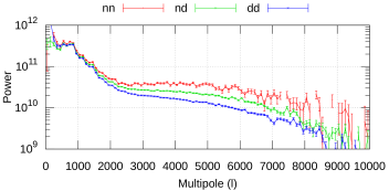
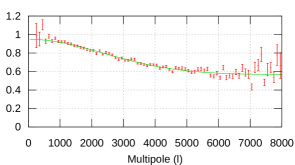
Figure 3: Left: Night-night (red), night-day (green) and day-day (blue) cross pseudo-spectra as a function of multipole for s18 PA5 f090 for the Day-N patch. The daytime loss in power on small scales is clearly visible. Right: The day/night relative beam inferred from the three spectra in each bin (red), and the smooth three-parameter model fit to it (green). See section 2.2.4 for details.

This approximate treatment of the daytime beam means that this data collection is of lower quality than the others. However, due to its high depth over a moderately large area it is still valuable for use cases that can accept O(10%) beam errors. The combined maps presented in this paper therefore come in two variants - night-only and day+night. The preliminary ACT daytime data cover three patches as described in table 1, for a total of 132 maps.

3 Co-adding maps

In principle, optimally coadding a set of maps is straightforward. We model the maps as noisy, transformed versions of a single underlying sky, $m$:

$$d =Pm+n,$$ (2)

where $d$ is a column vector containing the pixels from all the observed maps, $P$ is a response matrix that can encode beams, pixel windows or frequency differences, $m$ is a column vector containing the sky signal sampled at each pixel, and $n$ is the map noise, which we assume to be Gaussian with covariance $N$. Here, we will assume that each map has independent noise and that the only response difference we need to worry about is the beam. This results in the block-diagonal equation set:

$$\begin{pmatrix}m_{0}\\ m_{1}\\ \vdots\end{pmatrix} =\begin{pmatrix}B_{0}\\ B_{1}\\ \vdots\end{pmatrix}B_{\textrm{out}}^{-1}m+n, N =\begin{pmatrix}N_{1}&0&\cdots\\ 0&N_{2}&\cdots\\ \vdots&\vdots&\ddots\end{pmatrix},$$ (3)

where $B_{i}$ is the beam of map $m_{i}$, and $B_{\textrm{out}}$ is the beam we want the output map $m$ to have. The maximum-likelihood solution $\hat{m}$ to this equation system is given by:

$$(P^{T}N^{-1}P)\hat{m} =P^{T}N^{-1}d,$$ (4)

or equivalently

$$\sum_{i}\bar{B}_{i}^{T}N_{i}^{-1}\bar{B}_{i}\hat{m} =\sum_{i}\bar{B}_{i}^{T}N_{i}^{-1}m_{i},$$ (5)

where the relative beam is defined as $\bar{B}_{i}=B_{i}B_{\textrm{out}}^{-1}$. In the next subsections, we describe the approximation used to estimate $B_{i}$ (§3.1) and $N_{i}^{-1}$ (§3.2).

3.1 Beam Model

	Raw	Regularized
Beam transfer function

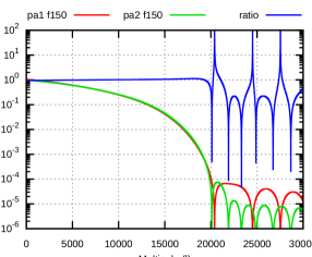
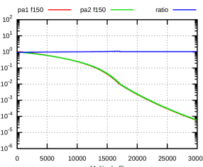
Figure 4: Left: The ACT PA1 and PA2 beams at f150, and their ratio. The ratio is quite constant up to $\ell=20000$, where the beam model breaks down and the ratio starts swinging wildly. Right: The same beams after regularizing them by replacing the values after they fall to 0.01 of the peak with a smooth function that preserves the beam ratio.

The Planck beams are slightly elliptical and slightly position-dependent (Planck Collaboration et al., 2014, 2016), but in the frequency range considered here they are reasonably well approximated as Gaussian, especially for $\ell<1500$ ($\ell<3000$ for f220) where the Planck data are relevant for this coadd. We used the following Gaussian FWHM beams from the Planck 2018 explanatory supplement: $9.66^{\prime}$ for f090, $7.22^{\prime}$ for f150 and $4.90^{\prime}$ for f220. These beams include the effect of the HEALPix pixel window to within the accuracy of the Gaussian approximation.

The ACT beam model is based on planet measurements and physical models of the optical system. Hasselfield et al. (2013) describes the basic approach used for the maps. Choi et al. (2020) describes recent improvements in removing the atmospheric contribution to the planet map and the inclusion of a scattering term from the primary surface deformations. These beam models are used as inputs.

These beam models break down at very high $\ell$ where the response becomes very low. This is illustrated in the left panel of figure 4, where two very similar beams and their ratios are plotted. The beams fall off smoothly as we approach $\ell=20\,000$, but then start oscillating messily around zero. If used directly, this would lead to an unphysical and wildly fluctuating beam ratio, which would translate into the map in question having its weight fluctuate by orders of magnitude from one multipole to another. As these oscillations occur on very small angular scales where the beam has suppressed all sky signal, we use a more well-behaved function: we replace the parts of the beam after the point $\ell^{*}$ where it falls to a fraction $v^{*}=10^{-2}$ of its peak value $B_{\textrm{max}}$ with $v^{*}B_{\textrm{max}}(\ell/\ell^{*})^{2\log(v^{*})}$. This extrapolation has the property that it preserves the ratio between two beams and matches both the value and first derivative of a Gaussian at the transition point. The result of applying this regularization to the beams is shown in the right panel of figure 4.

After regularizing each beam, we evaluate them at each pixel in 2D Fourier space using linear interpolation, and, in the case of MBAC, multiply it by the vertical ($f_{y}$) and horizontal ($f_{x}$) transfer functions (see section 4.3). The resulting 2D beams are divided by the desired 2D output beam to form the final relative beams $\bar{B}_{i}$.

3.2 Choosing the Noise Model

The inverse noise matrix $N^{-1}$ in equation 5 serves as the weight when averaging together the different data sets. Ideally it would be a full $N_{\textrm{pix}}$ by $N_{\textrm{pix}}$ matrix (with $N_{\textrm{pix}}\approx 10^{9}$) describing the full noise behavior, but due to the large number of degrees of freedom of such a matrix, this would be both hard to estimate and computationally infeasible to represent. We must therefore in practice approximate $N^{-1}$ using some simplifying assumptions. Thankfully, equation 5 does not rely on the value $N^{-1}$ for producing a bias-free map $\hat{m}$, only for its optimality, so we have considerable room for approximations.

3.2.1 Uncorrelated noise model

For maps with nearly white noise (e.g., WMAP and Planck), a good approximate description of the map’s inverse noise covariance is the uncorrelated noise model, where $N^{-1}$ is modeled as diagonal in pixel space, $N^{-1}\approx W^{-1}$, where W is a pixel-diagonal matrix representing the white noise variance of the map, which is often available as a mapmaker output, or can be estimated from the hitcount map. This noise model captures point-to-point changes in noise level, but cannot handle correlated noise such as that produced by the atmosphere.

uncorrelated	const covariance	const correlation

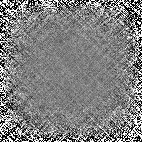
Figure 5: The uncorrelated noise model (left) can represent spatially inhomogeneous noise, but ignores all spatial correlations. The constant covariance noise model (middle) is the opposite, capturing complex spatial correlations but having no concept of position-dependence. The constant correlation noise model (right) combines these two models to allow for both correlation and inhomogeneity.

3.2.2 Constant covariance noise model

If maps have uniform but non-white noise spectra, then a reasonable approximation is the constant covariance noise model with $N$ approximated as diagonal in Fourier space, representing a position-independent 2D noise power spectrum. This model handles correlated and stripy noise well, but does not treat spatial variations in depth.

3.2.3 Constant correlation noise model

For a survey like ACT with spatially varying correlated noise, a better model for the noise is to describe it as a constant correlation pattern modulated by the inverse variance level, $N^{-1}\approx W^{-\frac{1}{2}}C^{-1}W^{-\frac{1}{2}}$, where $C^{-1}$ is a Fourier-diagonal matrix representing the 2D inverse correlation spectrum. Examples of these first three models are compared in figure 5.

The constant correlation approximation works well over small to medium size areas, like the 600 square degree ACT D56 patch, but it breaks down when the amount or direction of noise stripiness changes. This can happen due to scanning pattern variation (“fade” as illustrated in figure 6), or simply due to the sky’s curvature (“curved”). For example, in equirectangular cylindrical projection maps in equatorial coordinates, constant elevation scans trace out sine wave segments in the sky leading to a declination-dependent noise stripiness direction.

curved	fade

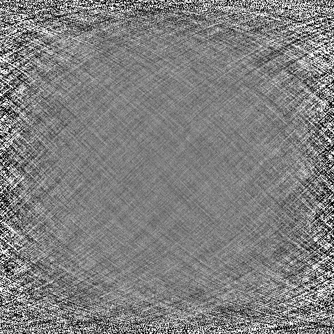
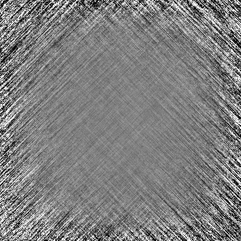
Figure 6: Examples of more complicated combinations of position-dependence and correlation patterns that cannot be represented by the constant correlation noise model. Left: Here the direction of the stripes is not constant, becoming shallower as we move up or down from the middle of the image. Right: Here the image goes from being dominated by /-stripes to \-stripes as we move from left to right.

3.2.4 Tiled constant correlation noise model

For this work, we extend the constant correlation noise model to large area maps so that we can model the position-dependent correlation pattern. The tiled correlation pattern approach used in this paper involves three steps:

1. Split the maps into equal-sized, overlapping tiles that are small enough that the constant correlation approximation is reasonably accurate. We chose a tile size of $4^{\circ}\times 4^{\circ}$ with $1^{\circ}$ of overlapping padding and a further $1^{\circ}$ of apodization to avoid implied wrap-around in the Fourier transforms. The resulting $8^{\circ}\times 8^{\circ}$ full tile and its overlap with neighboring tiles is illustrated in figure 7. Smaller tiles are better able to respond to fast changes in noise properties, while larger tiles let us model longer distance noise correlations and give us more statistical weight for building the per-tile noise model; $4^{\circ}\times 4^{\circ}$ is a compromise.

2. Solve equation 5 independently for each tile.

3. Use the overlap to seamlessly merge the coadded tiles into a single map (see section 5 and figure 13).

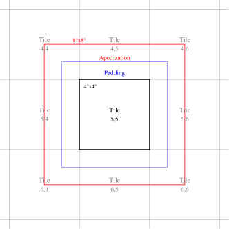
Figure 7: Illustration of our tiling scheme. The sky is tiled into $4^{\circ}\times 4^{\circ}$ degree tiles, but to ensure continuity in the solution and to make each tile Fourier-friendly we apply $1^{\circ}$ of padding (blue) and $1^{\circ}$ of apodization (red) to each tile, resulting in a set of overlapping $8^{\circ}\times 8^{\circ}$ tiles.

Figure 8: The input data sets that go into building the combined sky model for a given tile consist of a variable number of Stokes $IQU$ maps with corresponding inverse variance maps $W^{-1}$, all of which share a per-data-set beam. At the noise model estimation stage these are joined by a per-data-set inverse correlation matrix.

raw map	model	cleaned

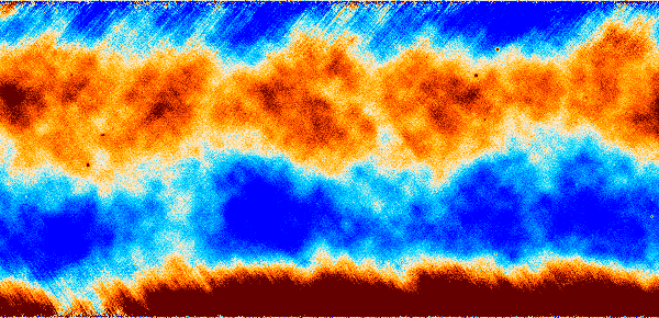
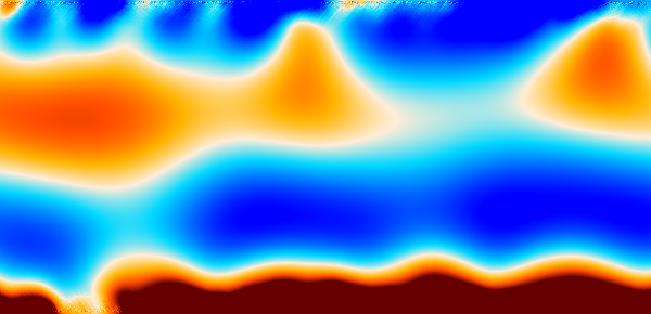
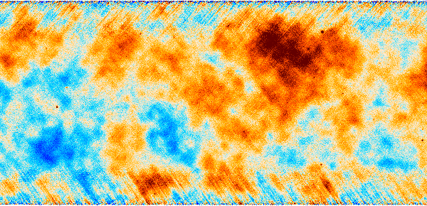
Figure 9: Left: A 10^∘x5^∘ section from the ACT MBAC f150 map showing an example of strong ground pickup, which shows up as mostly horizontal stripes that are usually stronger near the edge of the map. Middle: The maximum likelihood value for the pickup in the interior given the values in the outermost 60 pixels (half a degree) in the image. Right: The residual after subtracting this model. The pickup is almost completley removed, at the cost of some of the larger CMB scales.

4 Estimating the Constant Correlation Noise Model for Each Tile

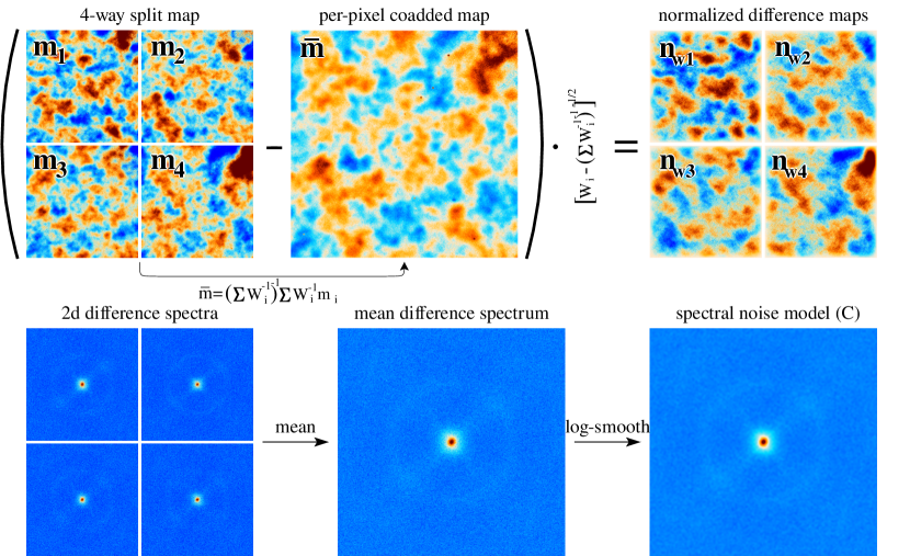
Figure 10: How the 2D noise correlation model $C(\vec{\ell})$ is built for an individual $8^{\circ}\times 8^{\circ}$ tile. Top: The inverse variance weighted average $\bar{m}$ of a set of map splits $\{m_{i}\}$ is subtracted from each split and then normalized by their expected white noise levels, resulting in a set of noise-only maps $\{m_{wi}\}$. The 4-way split map and per-pixel coadd shown here cover the same tile, but look quite different due to atmospheric noise. Bottom: The 2D power spectra of these noise-only maps are averaged together and smoothed to produce the final 2D noise correlation model. The horizontal and vertical axes of the plots in the bottom row are the horizontal wavenumber $\ell_{x}$ and the vertical wavenumber $\ell_{y}$, with the origin at the center. The central bright spot represents the atmosphere-dominated region at $\ell\lesssim 2000$, while the edge is at $\ell=21\,000$. Both the vertical and horizontal axes are linear. The color scale is linear at low values (blue), but becomes logarithmic at higher values (turquoise to red) to represent the large span in power.

After reading in the data for all data sets in a tile (see figure 8), some preparation is necessary before we can build their noise models and solve for the combined maps:

1. We expand all maps and inverse variances to full $TQU$ maps. For the T-only MBAC maps, the polarization inverse variance is set to zero, ensuring that they get zero weight, while the polarization signal maps are filled with white noise for convenience – having a non-zero signal here allows us to handle these maps on the same footing as the polarization maps from the other data sets without any special cases.

2. For all maps but Planck we apply a gentle detrending filter to remove excessive ground pickup from the edge of the maps (see figure 9). We assumed that the edge of the tile is dominated by some smoothly varying contaminant, and used this to in-paint the interior of the tile by solving for the maximum-likelihood value for the interior pixels given the value of the edge pixels. This was done by solving the system

   $$(V^{-1}+M^{-1})v=M^{-1}m,$$ (6)

   where $m$ is the data map and $v$ is the ground estimate we wish to construct. $M^{-1}$ is a pixel-diagonal matrix which is effectively a mask that selects the edge pixels as the reference values for the interpolation. It has value 0 in the interior and $1/(1$µK${}^{2})$ at the edge (though any value $\gg\textrm{max}(V^{-1})$ will work). $V^{-1}=\langle W^{-1}\rangle_{\textrm{pix}}/(1+((\ell+0.5)/1000)^{-3.5}$ represents a smoothly varying signal, with the smoothness governed by the constants 1000 and $-3.5$ in the expression. $W$ was defined in section 3.2.1. The result is quite insensitive to their exact values. The ones chosen here were based on the behavior of the ACT noise, but any spectrum with large correlations on the tile scale would work. Subtracting this ground estimate ($m\rightarrow m-v$) greatly reduces the ground pickup, at the cost of introducing a bias by removing some signal power. This is mostly on the scale of the tile size, i.e. 4^∘–8^∘, corresponding to $\ell\lesssim 100$, but smaller levels of bias extend up to higher $\ell$, falling below 0.5% at $\ell>1000$ (see appendix E). This ground subtraction was especially necessary for the MBAC maps. For the ACT+Planck maps, this loss of power at low $\ell$ is reduced due to the dominance of Planck there. In the future we will avoid this bias by replacing the ground filter with maximum-likelihood downweighting of the contaminated modes.

3. We clip the signal map values to the $\pm 100$ K range to avoid issues with extreme pixels. No real signal in the maps should be bright enough to be affected by this.

4. For each inverse variance map we compute $\gamma_{1}$, the median of its non-zero values, and $\gamma_{2}$, the median of the subset of its values that are larger than $10^{-5}\gamma_{1}$, and cap the inverse variance to $20\gamma_{2}$. The purpose of this is to avoid giving undue weight to (very rare) glitched pixels with unrealistically high inverse variance.

5. The edges of the survey areas see rapid changes in the noise properties which are difficult to model. Since these areas are quite noisy and do not contribute much information, we choose to suppress the lowest inverse variance areas via the transformation $W^{-1}\rightarrow W^{-1}\textrm{min}(1,W^{-1}/(0.2\gamma_{1}))^{5}$. Here $W^{-1}$ is the inverse white noise variance map, and the power of 5 was chosen to rapidly but smoothly suppress areas with too low exposure. This leaves areas with inverse variance greater than $0.2\gamma_{1}$ (effectively one fifth of the median of the exposed area) unchanged while rapidly damping lower values.

6. Fourier-space operations assume that periodic data inside each tile, but the real data contain power on scales larger than the tiles. If used directly in the per-tile Fourier transforms, this power would alias into every other multipole, which would show up as ringing patterns after applying any Fourier-space weighting operations. The standard solution to this problem is to smoothly taper off the data towards the edge of the map, in a process called apodization. We reserved a $1^{\circ}$ border at the edge of each tile for this purpose (see figure 7), and use it to apply a 60-pixel ($0.5^{\circ}$ at the equator) cosine taper to the edge of both the data map and $W^{-1}$ in each tile. We also apply a 60-pixel cosine taper at the edge of the exposed area in the case of data sets that stop part-way through a tile.

7. Any data set that ends up being empty after these steps is discarded for this tile.

As described in section 3.2, we model the map $m$ as having the inverse noise matrix $N^{-1}=W^{-\frac{1}{2}}C^{-1}W^{-\frac{1}{2}}$ in each tile. $W^{-1}$ is diagonal in pixel space and represents the inverse variance of the white part of the noise. This is approximately proportional to the number of times each pixel was observed, and was provided together with the sky maps for the data sets we analyze here. $C$ is taken to be diagonal in 2D Fourier space, i.e. $C_{\vec{\ell}\vec{\ell}^{\prime}}=\delta_{\vec{\ell}\vec{\ell}^{\prime}}C(\vec{\ell})$, with $C(\vec{\ell})$ being the 2D noise power spectrum of $m$ after factorizing out $W^{\frac{1}{2}}$. That is, $C(\vec{\ell})$ is the 2D noise power spectrum of $m_{w}=W^{-\frac{1}{2}}m$, which we will refer to as the normalized map.

In order to estimate $C(\vec{\ell})$ we construct noise-only maps by subtracting the inverse-variance weighted mean map $\bar{m}=(\sum_{i}W^{-1}_{i})^{-1}\sum_{i}W^{-1}m_{i}$ from each split $m_{i}$, resulting in noise maps $n_{i}=m_{i}-\bar{m}$. This is why we require several splits with independent noise in each data set. After taking into account the covariance of each map with the weighted mean map, we see that these difference maps have white noise variance $W_{i}-(\sum W_{i}^{-1})^{-1}$, allowing us to construct normalized noise maps $n_{wi}=\left[W_{i}-(\sum_{j}W_{j}^{-1})^{-1}\right]^{-\frac{1}{2}}n_{i}$. This procedure is illustrated in the top row of figure 10.

We then estimate the 2D noise power spectrum of each split as

$$C_{i}(\vec{\ell}) =\Big{|}\int d\vec{x}e^{-2\pi\vec{\ell}\cdot\vec{x}}n_{wi}(\vec{x})\Big{|}^{2}/g_{i}.$$ (7)

The extra correction factor $g_{i}$ is there to handle cases where some maps only partially cover the tile, leaving the rest of the tile empty. Normally variations in a data set’s depth across the tile would not be a worry at this stage, as we are working with the normalized noise maps $n_{w}$ where variations in depth have already been factored out. However, this fails for areas that have exactly zero depth ($W=0$). To avoid division by zero, any such unexposed areas are left as zero in $n_{w}$. However, this leads to a deficit of power in $C(\vec{\ell})$, which, if left alone, would result in data sets that only barely extend into a tile being given a disproportionally high weight. $g_{i}$ is a measure of the fraction of split $i$ that is not empty, and dividing by this undoes the effect of not being able to normalize unexposed areas. To be precise, we estimate $g$ as $g=\textrm{min}\Big{(}\langle W^{-1}>\gamma_{2}/100\rangle_{\textrm{pix}},\langle\alpha_{i}\rangle_{\textrm{pix}}\Big{)}$, where $\alpha_{i}$ is the total damping of $W^{-1}$ that was applied to split $i$ in steps 5 and 6, and where $\langle\rangle_{\textrm{pix}}$ denotes the mean over the tile pixels.

To summarize: $C_{i}(\vec{\ell})$ is the 2D noise power spectrum of the non-empty parts of the noise-only map $n_{i}$ after factorizing out variations in exposure time into $W_{i}$. Because we normalized the maps, these noise power spectra are dimensionless with values approaching unity in the white noise region.

We will assume that all splits of a data set have the same correlation structure, and only differ somewhat in their white noise properties. This lets us reduce sample variance in the noise power spectrum by averaging them, resulting in $C(\vec{\ell})=\frac{1}{N_{\textrm{split}}}\sum_{i}C_{i}(\vec{\ell})$.

4.1 Smoothing the spectrum

In order to suppress sample variance in our noise power spectrum estimate, we apply a Butterworth low-pass filter to the 2D power spectrum at a characteristic length scale of $\Delta\ell=400$. This corresponds to the last step in figure 10. Because the noise spectrum is a very steep function of $\ell$, we apply this smoothing in log-space and correct for the difference between normal averaging and log-averaging on the noise. We estimate this using simulations, and find that the log-smoothed power spectrum must be multiplied by 1.31 for a 2-way split and 1.14 for a 4-way split.

4.2 Down-weighting ACT at low $\ell$

The ACT maps are known to be missing power at low $\ell$ due to ground pickup filtering; bias from measuring the noise model from the same data it will be applied to ; and bias from stopping the iterative solution of the maps before the largest scales have converged (Aiola et al., 2020). These effects all mainly affect $\ell\lesssim 500$ in T and $\ell\lesssim 200$ in $P$, with the exception of the preliminary AdvACT maps, which currently have a few-percent loss of total intensity power for $\ell\approx 750/1200/1750$ at f090/f150/f220, with a gradually increasing loss below that. This is also the $\ell$-range where our noise spectrum becomes unreliable due to the smoothing performed in the previous section. In total intensity this hardly matters as Planck completely dominates by that point, but in polarization ACT is sensitive enough that some of these unreliable scales could slip through. To avoid this, we down-weight all ACT data by multiplying the inverse noise spectrum by $(1+(\ell/200)^{-10})^{-1}$. The effect of this is clearly visible in figure 17 as a cutoff of ACT at $\ell=200$.

4.3 Correcting for reprojection effects

Finally, we correct for the high-$\ell$ loss of power from reprojection. For Planck, we fill $\ell>6000$ with the mean noise power in the region $4500<\ell<6000$, emulating what the Planck noise power would have looked like if it hadn’t been truncated by being mapped at low resolution first.

We estimated the transfer function from the bicubic spline interpolation used when reprojecting MBAC by simulating a set of white noise maps for the two MBAC patches and applying the same interpolation to these. Because bicubic spline interpolation can be separated into independent vertical and horizontal interpolation steps, we can factorize this transfer function into a vertical and horizontal component $f_{y}(\ell_{y})$ and $f_{x}(\ell_{x})$, which we measure as the horizontal and vertical average of the square root of the mean power spectra of these interpolated simulations. These transfer functions are generally quite small, and only become noticable at high $\ell$. They deviate from 1 by 0.01% at $\ell=4\,000$, 1% at $\ell=10\,000$ and 10% at $\ell=16\,000$.

We divide out these transfer functions from $C$ by applying the transformation $C(\ell_{y},\ell_{x})\rightarrow C(\ell_{y},\ell_{x})/(f_{y}(\ell_{y})f_{x}(\ell_{x}))$ and also incorporate them into the 2D beam for MBAC. However, to avoid excessive deconvolution in MBAC-only areas ($<1\%$ of the survey area), we cap the transfer functions at 0.7 (which occurs at $\ell>20\,000$) and decrease the statistical weight of MBAC by a factor of 100 at multipoles where the transfer function was originally smaller. The effect of this is that any bias from ignoring part of the transfer function has no effect in the areas with any other ACT data present, while allowing a small bias in the form of extra smoothing in the small MBAC-only areas.

4.4 Example noise models

2D noise
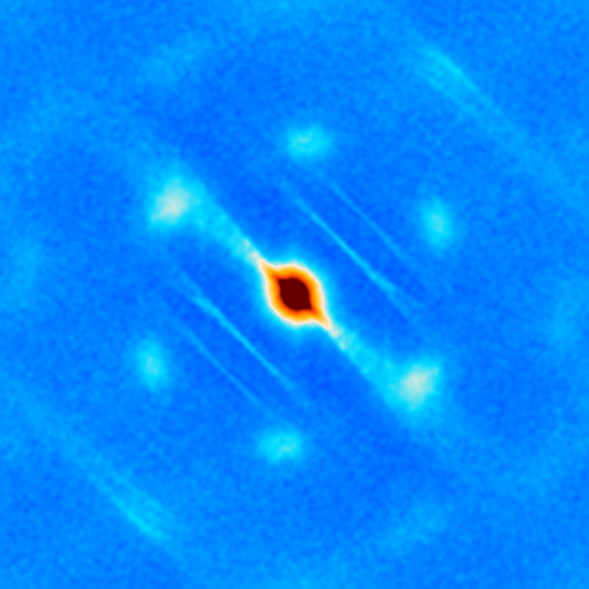
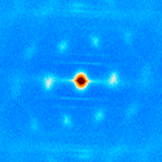
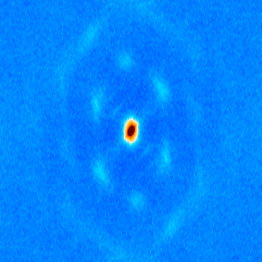
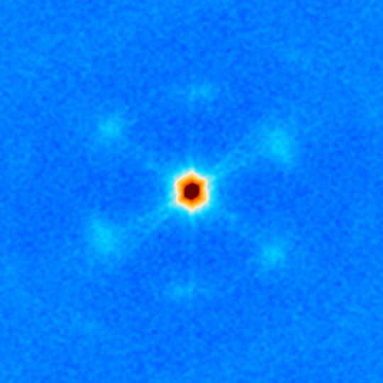
anisotropy

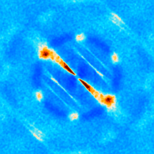
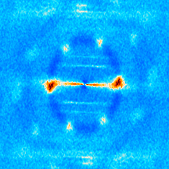
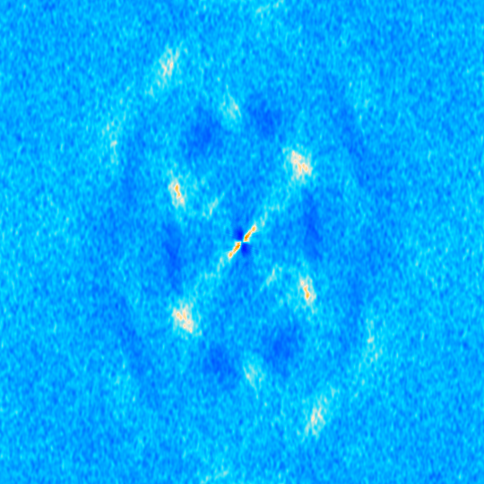
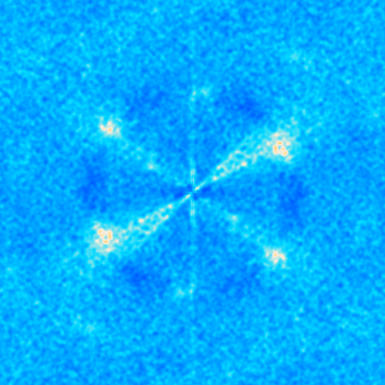
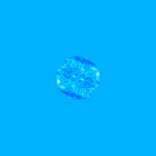
Figure 11: Top: Examples of the 2D noise correlation model $C$ that is built in section 4. The horizontal and vertical axes of each image corresponds to horizontal ($\ell_{x}$) and vertical ($\ell_{y}$) Fourier-modes respectively, with the origin at the center. Both axes are linear. From left to right these correspond to examples 1–5 in figure 12. The left-most two show examples of cases with very stripy noise due to low crosslinking; the next two have average levels of crosslinking, with roughly equal exposure in two roughly orthogonal scanning directions; and the last shows an example of Planck’s 2D noise power. Bottom: As the top, but with the radial average subtracted in order to highlight the anisotropy.

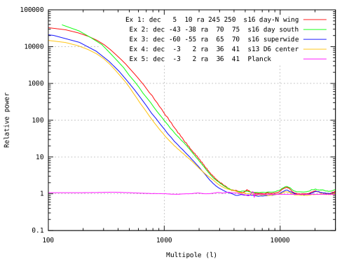
Figure 12: Radial averages of the total intensity 2D noise correlation model $C$ for the same cases as in figure 11. Example 1 (red) and 2 (green) have low crosslinking, leading both to anisotropic noise (as shown in figure 11) and higher large-scale power, as seen by these two curves being 2–3 times higher than the others for $\ell<3000$. Example 3 (blue) and 4 (orange) are both well crosslinked, but differ greatly in depth. Since the depth factorizes out into the $W$ term in the noise model, the depth is not distinguishable in $C$. Example 5 is Planck, which is almost completely flat due to the absence of atmospheric emission.

Figure 11 shows examples of the 2D correlation model $C$ for various data sets, showing the variety of noise correlation patterns. The central red spot is the atmosphere dominated region $\ell<3000$. Most of the survey area is well “crosslinked,” meaning that the telescope scans across each pixel in multiple different directions. In regions where this does not happen, the central atmospheric region stretches out to higher $\ell$ in a direction perpendicular to the scanning direction, as can be seen in column 1 of the figure. The hexagonal detector layout in the ACT focal plane manifests as a hexagonal pattern of spots in the 2D power spectrum because nearby detectors see nearby parts of the atmosphere, and hence become strongly correlated. The polarization power spectra, which are not shown here, are much flatter.

Radial averages for the same cases are shown in figure 12, illustrating the many order of magnitude increase in noise in the atmosphere-dominated range in ACT, compared to the almost white noise of Planck.

5 Constructing the Maps

After preparing the maps, noise model and beams in a tile, we are ready to solve equation 5 for the maximum-likelihood sky model. After inserting the form of the constant correlation noise model $N^{-1}=W^{-\frac{1}{2}}C^{-1}W^{-\frac{1}{2}}$ into the equation, it takes the form

$$\sum_{i}\bar{B}_{i}^{T}W_{i}^{-\frac{1}{2}}C_{i}^{-1}W_{i}^{-\frac{1}{2}}\bar{B}_{i}\hat{m} =\sum_{i}\bar{B}_{i}^{T}W_{i}^{-\frac{1}{2}}C_{i}^{-1}W_{i}^{-\frac{1}{2}}m_{i}.$$ (8)

This is a simple linear system that can be relatively efficiently solved using Preconditioned Conjugate Gradient iteration (PCG) (e.g. Shewchuk, 1994). With the Fourier-diagonal preconditioner $M=\Big{[}\sum_{i}\bar{B}_{i}^{2}\langle W_{i}^{-1}\rangle_{\textrm{pix}}C_{i}^{-1}\Big{]}^{-1}$ we found the solution to converge in 15–50 steps, depending on which maps go into the tile.

After solving for the maximum-likelihood sky map in each tile, we are left with merging these into a single consistent sky map. Ideally this would be as simple as cutting out the central, non-overlapping $4^{\circ}\times 4^{\circ}$ region of each tile and tiling them next to each other. This does work, but because each tile has its own noise model and hence weights the input maps slightly differently from its neighbors, this simple cropping+tile approach carries the risk of small discontinuities at the tile borders.

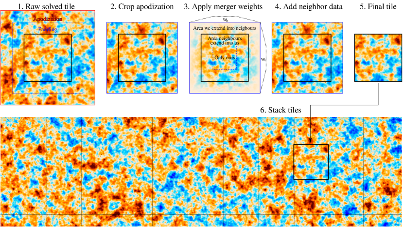
Figure 13: The tile merging procedure. Each raw solved tile contains a target $4^{\circ}\times 4^{\circ}$ degree region that would tile the sky, surrounded by $2^{\circ}$ of padding and $2^{\circ}$ of extra apodization, both of which overlap with neighboring tiles. We merge the tiles into a unified sky model by first cropping the unreliable apodization region, and then forming a weighted average of the overlapping regions. Finally, the central $4^{\circ}\times 4^{\circ}$ regions are stacked next to each other to form the full map. This procedure avoids tiny discontinuities that would arise from directly stacking the central $4^{\circ}\times 4^{\circ}$ of tiles that were solved with slightly different noise models.

To avoid such discontinuities, we instead only remove the $2^{\circ}$ apodization region of each tile, leaving us with the central $6^{\circ}\times 6^{\circ}$ region which still has substantial overlap with neighboring tiles. The overlap is resolved via bilinear crossfading: Each pixel in a tile is assigned a weight $w(\Delta x,\Delta y)=\omega(\Delta x)\omega(\Delta y)$ where $\Delta x$, $\Delta y$ is the offset from tile center, and where $\omega(x)=\textrm{min}(1,(3^{\circ}-|x|)/1^{\circ})$. This has the effect of assigning a weight of 1 to the central $2^{\circ}\times 2^{\circ}$ region of each tile (which does not overlap with any data from neighbors), and then linearly decreasing weight until it reaches 0 at the tile edge, which is a distance $3^{\circ}$ away from the tile center. The merged value of each tile is then the weighted average of it and the overlapping parts from its neighbors. This process is illustrated in figure 13. See appendix E for a validation of this procedure on simulations.

6 Map Properties

The final combined maps cover the area $0^{\circ}<\textrm{RA}<360^{\circ}$, $-62^{\circ}<\textrm{dec}<22^{\circ}$ in total intensity and linear polarization at f090, f150 and f220. Each map has variants with and without Planck, with and without daytime data and with and without point source subtraction. The maps cover a total of $43200\cdot 10320=446\cdot 10^{6}$ CAR pixels at 0.5 arcmin resolution, corresponding to 26 400 square degrees, of which roughly 70% falls within the ACT survey. The beam profiles of these maps are provided as part of the data release. They were chosen to be similar to the ACT beams to keep the amount of reconvolution low, and are therefore not Gaussian. They have full-widths at half-maxima of 2.1/1.3/1.0 arcmin at f090/f150/f220.

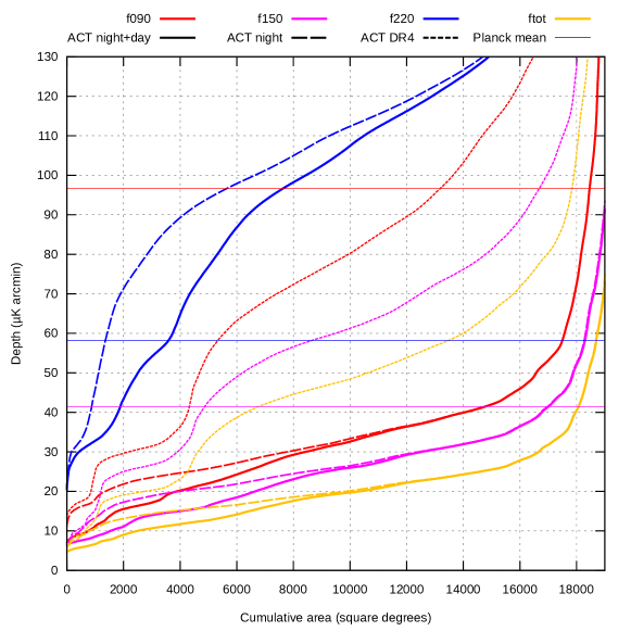
Figure 14: The white noise levels for the ACT-only coadds presented here, compared to that of ACT DR4 (dotted) and the average Planck map depths (horizontal lines). The curves show the total area of the survey with noise at a given level or lower. For example, these maps have 12 000 square degrees where the noise level does not exceed 30 µK-arcmin at f150. Alternatively, this graph can be interpreted as a cumulative distribution function for the map depth if the axes are transposed. The day+night (solid) and night-only (dashed) curves converge at the largest areas because the daytime data only contribute to a small subset of the survey area.

Figure 14 shows the cumulative total intensity white noise depth distribution of the ACT-only maps. This is the noise level appropriate at high $\ell$ where atmospheric fluctuations are sub-dominant (see figure 16). The maps span a wide range of depths, with 2500 square degrees deeper than 10 µK-arcmin, 6500 square degrees deeper than 15 µK-arcmin, 10 000 square degrees deeper than 20 µK-arcmin, 15 000 square degrees deeper than 25 µK-arcmin and 19 000 square degrees deeper than 70 µK-arcmin when combining the three frequencies. Over most of the survey area, these maps are $2.3/2.6/\infty$ times deeper than ACT DR4 at f090/f150/f220 (see appendix C); and they are deeper than the mean Planck depth over 19k/17k/4k square degrees. The polarization noise level is approximately $\sqrt{2}$ higher.

f090
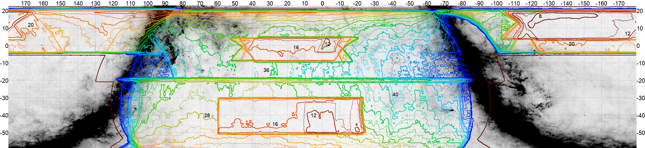
f150
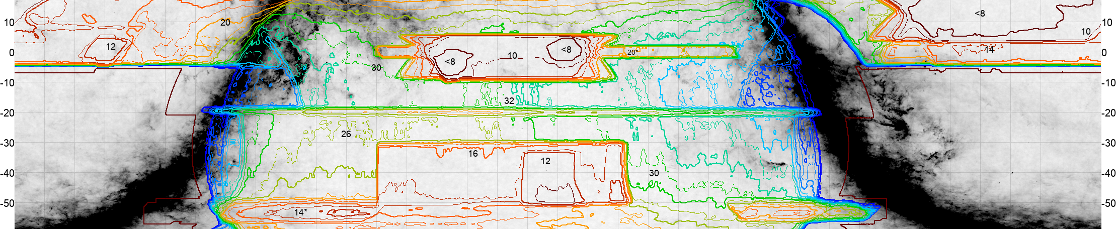
f220

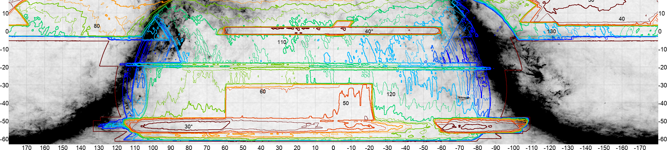
Figure 15: Spatial distribution of ACT-only map depths for the three different ACT frequencies, as shown by iso-depth contours that go from 8/8/30 µK-arcmin (red) to 60/50/180 µK-arcmin (blue) with contour intervals of 2/2/10 µK-arcmin for f090/f150/f220 respectively. This covers most of the depth range in the maps, though there are areas that are somewhat deeper or shallower. The outermost red curve shows the full outline of the survey area. Selected contour lines are labeled with their depth to make it easier to read off values. These are T noise levels; Q and U are approximately $\sqrt{2}$ higher. They also only describe the noise level at small scales. The background grayscale map is the dust-dominated Planck 353 GHz map.

Figure 15 shows the spatial distribution of the map depths overlaid on the dust-dominated Planck 353 GHz map. The deepest region is the Day-N region centered on RA = -145^∘, which is deeper than 8 µK-arcmin at both f090 and f150; followed by the night-only regions D5, D6 and D56 that were the focus of ACT DR2 and ACT DR3. The ACT observing strategy does not target the galaxy, but some of it is still hit due to limitations in the scanning pattern implementation, in particular the region around RA = 90^∘, which includes the Orion nebula.

	f090	f150	f220
D6
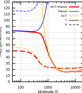
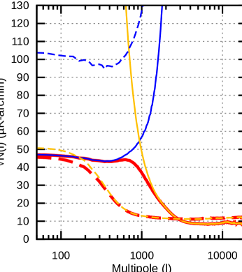
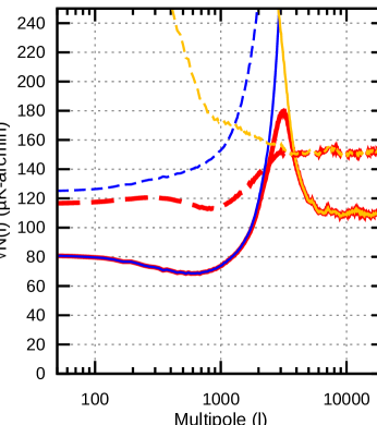
Day-N
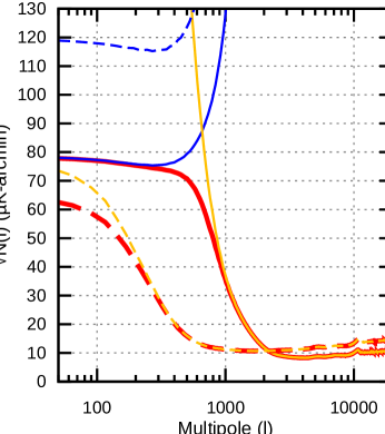
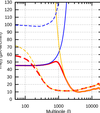
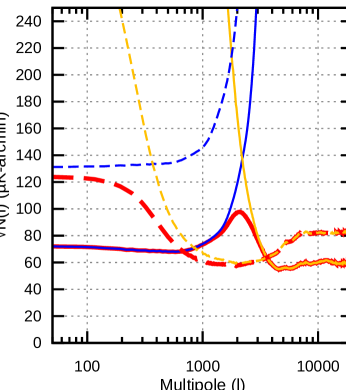
AA

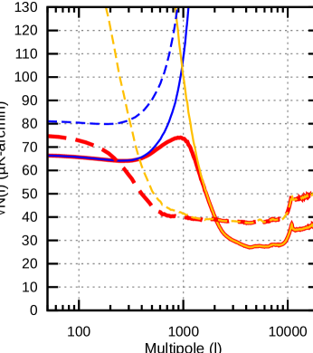
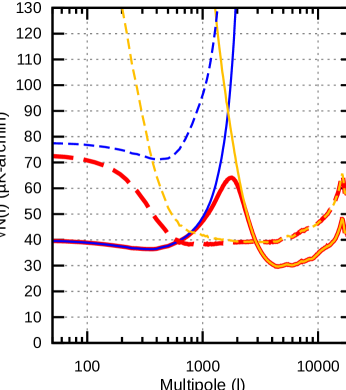
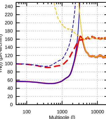
Figure 16: The angular noise spectra of ACT+Planck (thick red), Planck only (blue) and ACT only (yellow) in total intensity (solid) and polarization (dashed). The columns represent the f090, f150 and f220 frequency bands from left to right. Each row corresponds to a 10^∘x10^∘ patch centered on different locations on the sky. D6: $32^{\circ}<\textrm{RA}<38^{\circ}$, $-8^{\circ}<\textrm{dec}<2^{\circ}$, the middle of the deep, night-time only patch “D6” from ACT DR2-DR4. Day-N: $230^{\circ}<\textrm{RA}<240^{\circ}$, $8^{\circ}<\textrm{dec}<18^{\circ}$, part of the deep northern daytime patch. AA: $-5^{\circ}<\textrm{RA}<5^{\circ}$, $-25^{\circ}<\textrm{dec}<-15^{\circ}$, an area representative of the wide, shallow Advanced ACT survey area. The noise curves shown are the square root of the noise spectra in units µK arcmin to make it easier to compare with the depth maps. The Planck noise blows up at high $\ell$ due to its large beam. The ACT noise blows up at low $\ell$ due to the atmosphere – this happens at lower $\ell$ in polarization due to strong suppression of the atmosphere there. The high-$\ell$ upturn seen in some of the plots is caused by significant contribution from data with larger beam than the output beam, resulting in net deconvolution.

D6	Day-N	AA

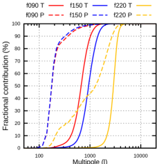
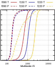
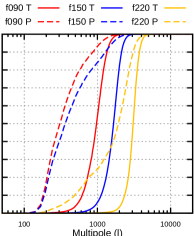
Figure 17: The fractional contribution of ACT to the ACT+Planck coadd as a function of angular scale for the same three patches as in figure 16. This is only approximate, as the real weights are anisotropic and position-dependent and hence can’t be represented as a simple function of scale. The transition from Planck to ACT dominance is driven both by the Planck beam size and the ACT atmospheric 1/$\ell$ noise, as seen in figure 16. Note: D6 is much shallower in f220 than the other bands. In shallow areas, ACT dominates at $\ell>1000/1700/3000$ in T and $300/360/1700$ in P, for f090/f150/f220. In deep areas these numbers are about 1/3 lower.

The map white noise depth gives an incomplete picture of the map noise properties due to the strongly scale-dependent atmospheric noise in the ACT maps, as shown in figure 16. This noise has an $\ell_{\textrm{knee}}$ of about 2000/3000/4000 in total intensity and 500/500/700 in polarization at f090/f150/f220, and increases rapidly ($N_{l}\propto\ell^{-3}$) below that. When coadding with Planck this rise stops at the Planck noise level, resulting in maps with much flatter noise curves. This noise behavior is reflected in the weights ACT and Planck data get in the combined maps. While the full weights are defined in a hybrid of Fourier space and pixel space, we can approximate them as simple functions of $\ell$ in limited areas. Figure 17 uses this to show the approximate fractional contribution of ACT to the ACT+Planck coadd as a function of angular scale in three different areas of the sky.

6.1 Coarse-grained noise model

In addition to the purely spatial (figure 15) and purely angular scale (figure 16) slices through the noise model, we also compute the approximate inverse noise variance $\tilde{N}^{-1}$ in units of $1/$µK² per full-resolution (0.5 arcmin) pixel as a function of position in the map (sampled at every 0.5^∘ in RA and dec), multipole (50 logarithmically spaced multipoles from 100 to 18000), detector array (e.g. ACT MBAC AR1, ACTPol PA3 f090 or Planck 217) and Stokes parameter (I, Q, U). These files are labeled “noisebox” in the data release.

6.2 Bandpasses

No attempt is made to correct for the bandpass differences between the individual maps in each bandpass group (see figure 2). This results in somewhat scale-dependent effective bandpasses and band-center, with the main feature being the transition fromPlanck-dominance to ACT-dominance around $\ell\sim 1000$ in the ACT+Planck maps (see figure 17). To estimate how large an effect this is, we first normalize the bandpasses for all detector arrays in figure 2 to units of µK/(MJy/sr)/GHz to make them comparable to each other:

$$f(\ell,\nu) =\frac{f^{\textrm{raw}}(\ell,\nu)}{\int d\nu^{\prime}f^{\textrm{raw}}(\ell,\nu^{\prime})\delta B(\nu^{\prime})}.$$ (9)

Here $\nu$ is the frequency of the light, $B(\nu,T)$ is the black-body spectrum of the CMB in MJy/sr, $\delta B(\nu)=\frac{\partial B(\nu^{\prime},T)}{\partial T}\Big{|}_{T=2.725K}$ is the spectral response to CMB temperature fluctuations, and the normalization is based on the fact that all maps are defined to have unit response to these fluctuations since they are in linearized CMB temperature units. $f^{\textrm{raw}}(\ell,\nu)$ is the unnormalized bandpass for each array. This is scale-dependent (a function of $\ell$) because the telescope beams get slightly sharper towards the high-frequency end of each bandpass. Assuming a beam size that scales as $1/\nu$, as for a normal diffraction limited system, we get

$$f^{\textrm{raw}}(\ell,\nu) =f^{\textrm{raw}}(\nu)B\Big{(}\ell\frac{\nu_{0}}{\nu}\Big{)}$$ (10)

where $B(\ell)$ is the instrument beam and $\nu_{0}=\frac{\int d\nu f^{\textrm{raw}}(\nu)\delta B(\nu)}{\int d\nu\delta B(\nu)}$ is the effective beam band-center for CMB fluctuations.

Given these normalized per-array bandpasses we can find the effective bandpass for Stokes component $s$ at position ($\alpha$,$\delta$) and multipole $\ell$ in the map as the inverse variance weighted average over the arrays $i$,

$$f^{\textrm{eff}}(s,\ell,\alpha,\delta,\nu)=\frac{\sum_{i}f_{i}(\ell,\nu)\tilde{N}^{-1}(s,i,\ell,\alpha,\delta)}{\sum_{i}\tilde{N}^{-1}(s,i,\ell,\alpha,\delta)}$$ (11)

Figure 18 shows the mean and standard deviation of $f^{\textrm{eff}}$ when averaged over the whole survey area and all scales. The bandpass varies at the $\sim 15\%$ level in the ACT-only maps, but this only results in a $\sim 0.5\%$ variation in the band-center. For the ACT+Planck maps the bandpass still varies by $\sim 15\%$ across positions and scales on the map, but there is now a 2–5% difference between the bandpass at large ($\ell\lesssim 1000$) and small ($\ell\gtrsim 1000$) scales (figure 18 right panel). As seen in figure 19, the ACT+Planck map’s response to individual components like tSZ, synchrotron or dust has a position-dependence of O(1%). If more accurate control over bandpasses is needed, they can be evaluated at any needed multipole and position using equation 11 (see appendix A.4).

ACT+Planck bandpasses	ACT+Planck band centers
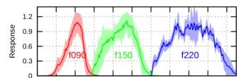
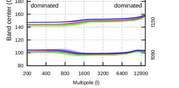
ACT only bandpasses

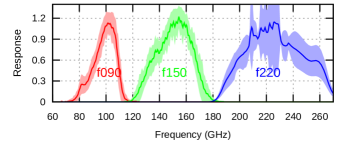
Figure 18: Left: The average bandpass of the ACT+Planck (top) and ACT-only (bottom) combined maps normalized to a peak of $\approx 1$ to make them easier to plot on the same scale. The colored band shows the $\pm 1\sigma$ inverse variance weighted variation of the bandpass across positions and scales in the maps. Right: The sky-averaged band-center of the ACT+Planck maps as a function of multipole. The transition between Planck-dominance and ACT-dominance is clearly visible at $\ell\sim 1000$, and represents a 2–5% shift. The band around each curve shows the variation of the bandcenter across the sky. The band-center is computed for a CMB spectrum (red), synchrotron spectrum (green, $\propto\nu^{-0.5}$) and dust (blue, modified blackbody with $T=19.6$K and $\beta=1.59$). The frequency-dependence of the beam (slightly higher resolution at the high end of the band than the low) is taken into account, and leads to a slight up-tilt of the band-centers at high $\ell$.

f090	f150	f220

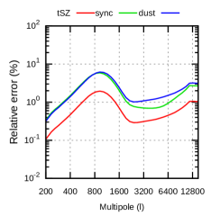
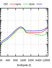
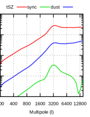
Figure 19: The relative standard deviation (standard deviation divided by the mean) of the ACT+Planck map’s response to the thermal Sunyaev Zel’dovich effect (red), synchrotron (green) and dust (blue) as a function of the multipole ($\ell$) at f090 (left), f150 (middle) and f220 (right) when averaged across the survey area with the inverse noise model as weights. The response typically varies by about 1% across the map. The high value for tSZ at f220 is due to the insensitivity of f220 to tSZ. This figure takes into account the frequency-dependence of the beam (the resolution is slightly higher at the high frequencies of a bandpass than the low frequencies), but does not include the overall calibration uncertainty of the map, which is O(1%). The CMB itself is not included because the maps are calibrated to the CMB, which causes all its response uncertainty to be in the gain calibration rather than the bandpasses. The synchrotron and dust spectra used here are the same as in figure 18.

6.3 Caveats and limitations

1. These maps include preliminary data from the 2017–2018 seasons of Advanced ACT, and while a fair amount of work has gone into characterizing them, they have not yet been subjected to all the tests of a proper ACT cosmological data release, and gain/beam errors of several percent should be expected. This is doubly true for the daytime maps, where there is a position-dependent beam FWHM uncertainty of O(10%).

2. As part of the solution process, the input maps are reconvolved to a common target beam. For some parts of the sky this resulted in a net beam deconvolution, leading to an upwards slope of the high-$\ell$ noise spectrum. This is seen in the AA patch in figure 16, for example. This “blue” noise does not represent an actual noise excess; it is simply a result of the choice of output beam. If white noise is desirable, one can simply reconvolve the maps to a slightly bigger beam.

3. Many use cases benefit from having split maps made from independent subsets of the data in order to properly account for the noise properties. We do not provide such splits for the coadded maps we present here. In theory, we could make these by splitting each data set in two, and making one coadded map from all the first halves and another from all the second halves. However, because the noise model requires at least two splits, this requires us to have at least 4 splits for all the initial data sets, and this is not the case for large parts of our data set (see section 2.2). We hope to improve on this in a future combined map, either by greatly reducing the number of degrees of freedom in the noise model, or by coadding a set of noise simulations of the individual input maps.

4. As discussed in section 6.2, no attempt is made to correct for the bandpass differences between the individual maps, resulting in a mild position dependent (0.5%) and scale dependent (2–5% if Planck is included, otherwise 0.5%) effective band center.

5. The ACT-only maps have a total intensity deficit at $\ell\lesssim 750/1200/1750$ for f090/f150/f220 due to the contribution from the preliminary Advanced ACTPol maps, which are not yet up to the standard of the earlier ACT maps. This should have little impact on the ACT+Planck maps since Planck dominates for $\ell<1000/1700/3000$ in the shallow areas where the preliminary Advanced ACTpol maps make up the dominant ACT contribution.

6. There is a further low-$\ell$ loss of power from the ground filter we apply to all ACT maps (see figure 9), which also mostly affects $\ell<1000$ ($<0.5$% above that, but growing to 10% by $\ell=350$, see appendix E). This is again mitigated, but not eliminated, by the presence of Planck data in the ACT+Planck coadds.

7 Map Images and Features

The main products of this paper are multi-frequency temperature and polarization maps that have the resolution and sensitivity of ACT on small scales and the simple noise properties and sensitivities of Planck on large-scales.

Figure 20 shows the total intensity (T), linear polarization (Q, U) and divergence (E) and curl fields (B) (Zaldarriaga & Seljak, 1997) for a simple pixel-space average of the f090 and f150 maps in a 772 square degree patch covering most of the deep Day-N field. The effective noise level in this patch is 7.1 µK-arcmin. The polarization Q/U maps show the clear +/x pattern indicative of high S/N E-modes, which is confirmed in the E-mode map itself. The B map is consistent with noise (and small amounts of ground pickup near the top) with the exception of a few polarized point sources that show up as quadrupoles due to the non-local nature of E and B.

T
Q
U
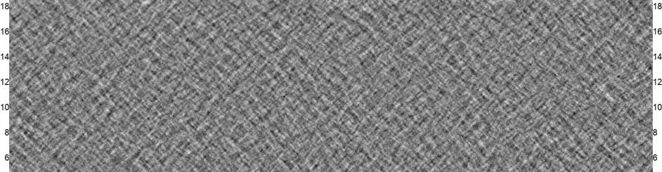
E
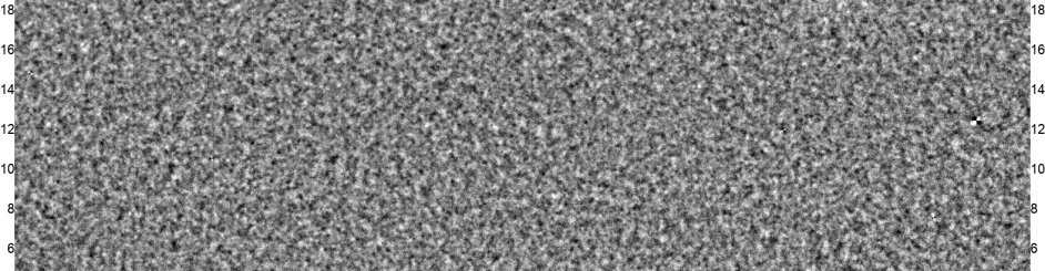
B

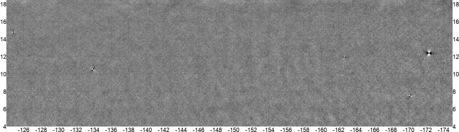
Figure 20: A 772 square degree patch covering $-175<\textrm{RA}<-124$ and $4<\textrm{dec}<19$, one of the deepest areas in ACT. From top to bottom the panels show the temperature T, linear polarization Q and U, and the corresponding polarization gradient and curl fields E and B for a day+night coadd of f090 and f150. Planck is included in T, where it mainly affects scales larger than about half a degree. The other panels are ACT-only, but would not be noticeably different with Planck. The E map is clearly signal-dominated, while B is consistent with noise, aside from a few polarized point sources that show up as small quadrupoles. The color range is $\pm 500$ µK in T (top) and $\pm 20$ µK in the others.

Figure 21 shows the same f090+f150 E and B fields over a much larger area covering 9 500 square degrees (23% of the sky and a bit more than half the full ACT area). On this length scale the characteristic E-mode length scale appears small enough that they could be mistaken for noise, but the difference between the E and B maps shows that the E-modes are signal dominated even in the shallower parts of our survey.

E
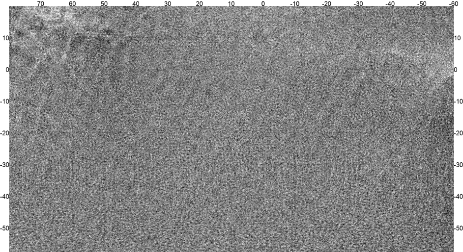
B

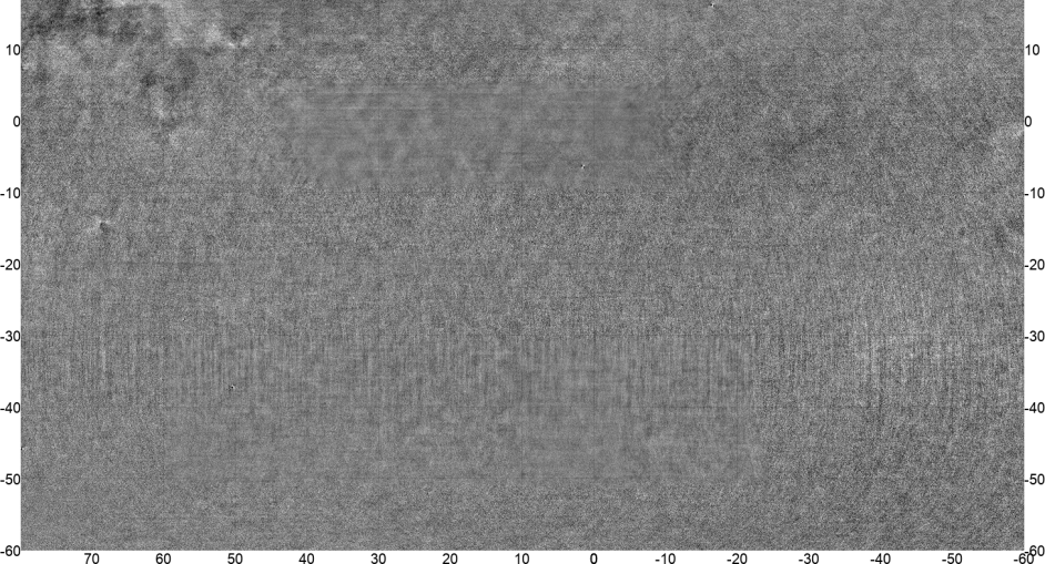
Figure 21: A 9690 square degree patch covering $-60<\textrm{RA}<80$ and $-60<\textrm{dec}<20$, 23% of the sky and a bit more than half the full ACT area. Aside from a few deeper patches, this represents the shallowest parts of our survey. The top/bottom panel show E/B-modes for a f090+f150 ACT+Planck coadd. This includes daytime data in the areas where it exists, but 87% of this area is night-only. Despite the shallowness of this area, E-modes around $\ell=500$ are still signal dominated. At this multipole Planck contributes roughly 20% of the weight. This gradually increases at lower $\ell$, and starts to dominate for $\ell<150$. Some galactic dust contamination is visible near the edges of the map.

Figure 22 applies a matched filter for point sources to the ACT f090 map in a $4^{\circ}\times 4^{\circ}$ degree sub-patch of Day-N, revealing more than 45 point sources and 20 clusters in a 16 square degree area. The point source and cluster potential of these maps will be explored in two upcoming papers, but a preliminary search has 4 000 confirmed clusters (Hilton et al., 2020, in prep) and 18 500 point source candidates at $>5\sigma$. For comparison, the largest published point source catalog at these frequencies is Everett et al. (2020) with 4845 point sources at $>4.5\sigma$, and the largest published SZ-detected cluster catalog, PSZ2, has 1203 confirmed clusters (Planck Collaboration, 2016b).

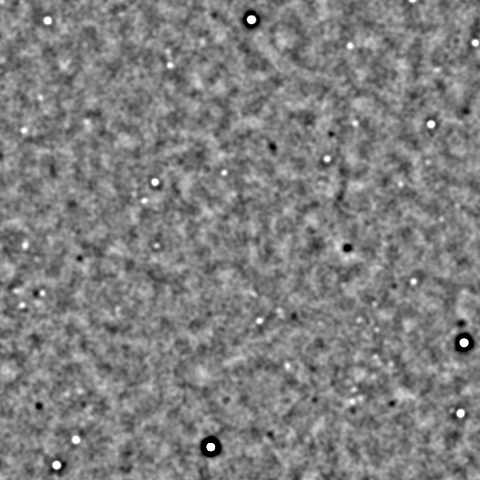
Figure 22: The ACT f090 day+night map filtered to enhance point sources, clusters and other small-scale features. The region shown is a $4^{\circ}\times 4^{\circ}$ square centered on RA = 224.5^∘, dec = 6^∘. More than 20 clusters are visible as temperature decrements (dark) through the tSZ effect, and more than 45 point sources are visible as temperature increments (light). This is one of the deepest ACT regions, with a depth of about 9 µK-arcmin (0.6 mJy) in this band. The filter used here is approximately matched to the beam profile and atmospheric correlation structure, and is more optimal for point sources than for clusters.

As seen in figure 15, ACT has partial coverage of the galactic plane. About 1/3 of the disk is covered at very shallow ($>60$ µK-arcmin but still strongly signal-dominated) depth, barely including the galactic center. Additionally, the area with galactic longitude $190<\ell<245$ (including e.g. the Orion and Rosette nebulae) is covered at depths of 16–60 µK-arcmin typical of shallow-to-medium CMB areas. Compared to Planck alone, ACT’s $5\times$ higher resolution reveals much more of the small-scale structure of the dust (see figure 23) without needing to extrapolate from the much higher frequencies of e.g. WISE (Meisner et al., 2017).

	f090	f150	f220
ACT+Planck
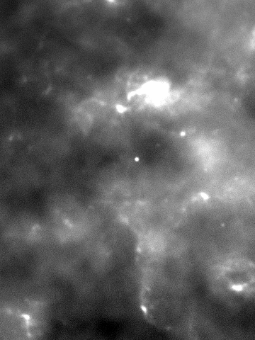
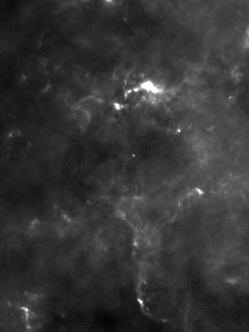
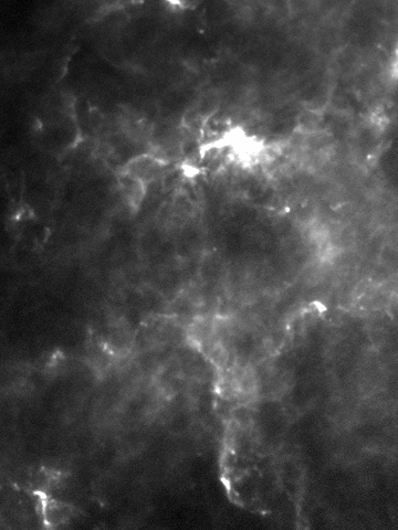
Planck

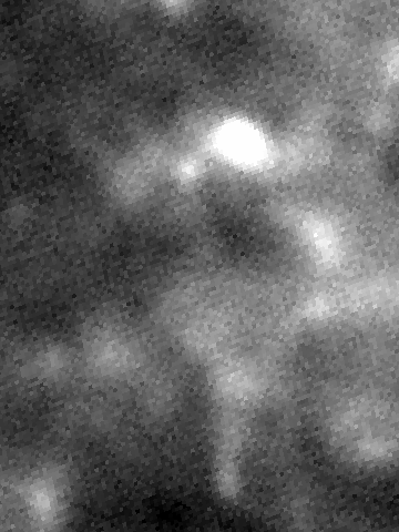
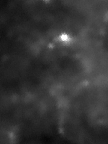
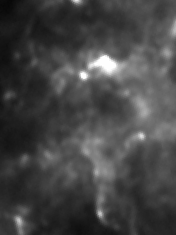
Figure 23: Comparison of ACT+Planck and Planck alone in the region $95^{\circ}>\textrm{RA}>93^{\circ}$, $15^{\circ}<\textrm{dec}<19^{\circ}$ in the galactic plane. ACT’s $5\times$ higher resolution than Planck allows for high-resolution dust science at CMB-relevant frequencies.

Finally, figure 24 gives some examples of other miscellaneous objects one can find in the maps, including radio lobes from active galaxy Fornax A, the Helix planetary nebula, resolved nearby galaxies including the Leo Triplet, NGC 55 and NGC 253, merging clusters detected through their asymmetric tSZ signal, and the individual stars Mira, Betelgeuse and $\pi^{1}$ Gruis. These images suggest the wealth of new information that is present in these new publicly available maps.

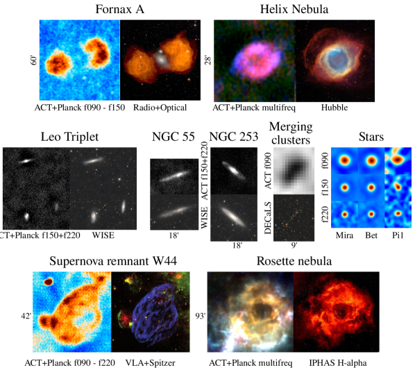
Figure 24: Some nearby objects that can be found in these maps. The small numbers next to each set of images indicates the length of the corresponding side in arcminutes. Top left: Fornax A (NGC 1316). The CMB was removed by subtracting f150 from f090. Compared to a radio + optical composition by Fomalont et al. (1989, 2005). The central galaxy is visible in individual frequencies, but was cancelled in this difference map. Top right: The Helix Nebula (NGC 7293, The Eye of God/Sauron). Here f090, f150 and f220 were scaled until they had roughly the same noise level, and then assigned to the red, green and blue color channels respectively. Compared to a famous Hubble image of the same object (NASA et al., 2003). Middle left: The Leo Triplet (M65, M66, and NGC 3628) from a pixel-space sum of ACT+Planck f150 and f220, compared to unWISE W1/W2 (Meisner et al., 2017). Middle center-left: As the Leo Triplet, but for NGC 55 (the Whale Galaxy) and NGC 253 (the Sculptor galaxy). Middle center-right: Example of a merging galaxy cluster pair that appears clearly elongated both to ACT (tSZ) and DECaLS (stars) (Dey et al., 2019). Middle right: Several large, nearby stars are detectable as significant mm-band sources by ACT. Shown here are filtered images of three examples: Mira, Betelgeuse and $\pi^{1}$ Gruis. Other strong detections include V0711 Tau and RV Aqr. Bottom left: The supernova remnant W44. Galactic dust was reduced by subtracting f220 from f090. The comparison image shows a composite of images from radio (VLA 324 MHz, in blue) and infrared (Spitzer 8 µm and 24µm, in green and red, respectively) from Castelletti et al. (2007). Bottom right: The Rosette nebula. f090, f150 and f220 are mapped to the red, green and blue channels respectively. Compared to an H$\alpha$ (656.28 nm) image prepared by Wright (2007) using data from IPHAS (Barentsen et al., 2014).

8 Conclusion

We have presented a method for combining maps with greatly varying sky coverage, depth and angular resolution and spatially varying anisotropic noise into a near-optimal sky map.

We used this to combine 270 ACT maps representing observations from 2008 to 2018 into three frequency maps, centered at roughly 90 GHz, 150 GHz and 220 GHz. These maps cover more than 19 000 square degrees (46% of the sky), and include previously unreleased preliminary data from the two first seasons of Advanced ACTPol. We also provide a second set of maps that also include the more challenging ACT daytime data, which provide a large boost in depth over a 3 000 square degree subset of the survey area.

In addition to these ACT-only maps, we also produce versions that have been combined with the nearest-frequency Planck HFI maps. This has the effect of filling in the large angular scales ($\ell\lesssim 1000$) that ground-based millimeter surveys like ACT have trouble measuring due to the influence of the atmosphere, resulting in a map that covers scales from $180^{\circ}$ to $\sim 1$ arcmin.

We make these maps available to the public in the hope that they will be useful, but caution that due to the preliminary nature of some of the component data sets, these maps should not be used for precision cosmological analysis, and the version of the maps that include daytime data in particular should only be used for cases that can tolerate a position-dependent O(10%) beam uncertainty. The effective band-center is also somewhat scale-dependent due to differences in the bandpasses of the individual input maps.

In Hilton et al. (2020) we use these maps to find 4 000 confirmed clusters through the thermal Sunyaev Zel’dovich effect, and in a second upcoming publication we detect 18 500 millimeter point sources at $>5\sigma$, both substantial improvements on the state of the art. Other anticipated use cases include tSZ and kSZ cluster stacking and CMB cluster lensing measurements. The maps also include hundreds of resolved galaxies and polarized point sources; cover about 1/3 of the galactic disk at high resolution; and also include several classes of objects one would not normally associate with a map from a CMB survey, including radio lobes from active galactic nuclei, planetary nebulae and even a few individual stars.

The cosmological analysis of an expanded and fully calibrated version of this data set, including CMB and lensing power spectra and cosmological parameters, will be the subject of a future ACT data release.

Appendix A The data release

A.1 Sky maps

The main data products in this data release are the ACT+Planck  and ACT-only sky maps:

act_planck_dr5.01_s08s18_AA_f090_night_map.fits
act_planck_dr5.01_s08s18_AA_f150_night_map.fits
act_planck_dr5.01_s08s18_AA_f220_night_map.fits
act_planck_dr5.01_s08s18_AA_f090_daynight_map.fits
act_planck_dr5.01_s08s18_AA_f150_daynight_map.fits
act_planck_dr5.01_s08s18_AA_f220_daynight_map.fits
act_dr5.01_s08s18_AA_f090_night_map.fits
act_dr5.01_s08s18_AA_f150_night_map.fits
act_dr5.01_s08s18_AA_f220_night_map.fits
act_dr5.01_s08s18_AA_f090_daynight_map.fits
act_dr5.01_s08s18_AA_f150_daynight_map.fits
act_dr5.01_s08s18_AA_f220_daynight_map.fits

These are 32-bit float FITS images with shape 43200,10320,3. The first two axes are RA and dec in the Plate Carreé projection, covering the area $180^{\circ}>\textrm{RA}>-180^{\circ}$ and $-63^{\circ}<\textrm{dec}<23^{\circ}$ at 0.5 arcmin resolution. The last axis represents the three Stokes parameters I, Q and U in the Healpix/Cosmo polarization convention. The maps are in units of µK CMB temperature increment. Note that the axes appear in the opposite order when loaded as a pixell enmap, since enmap (like numpy) uses row-major ordering instead of column-major ordering like FITS does.

A.2 Inverse variance maps

Associated with each of these maps is a noise floor inverse variance map, which has the same shape and contains an estimate of the non-atmospheric inverse variance in µK^-2 per pixel. This does not include the contribution from Planck due to Planck’s limited multipole range. These files are labeled ivar, e.g. act_dr5.01_s08s18_AA_f090_night_ivar.fits.

A.3 Detailed noise model

A more detailed noise model is provided in the files

act_planck_dr5.01_s08s18_AA_f090_night_fullivar.fits
act_planck_dr5.01_s08s18_AA_f150_night_fullivar.fits
act_planck_dr5.01_s08s18_AA_f220_night_fullivar.fits
act_planck_dr5.01_s08s18_AA_f090_daynight_fullivar.fits
act_planck_dr5.01_s08s18_AA_f150_daynight_fullivar.fits
act_planck_dr5.01_s08s18_AA_f220_daynight_fullivar.fits

These are 32-bit float FITS images with shape 720,172,50,15,3, and provides the noise inverse variance in units of µK^-2 per square arcmin as a function of position, $\ell$ and detector array, albeit at reduced resolution to make the file size managable.

The first two axes are RA, dec in the same projection as the main maps, but at only 0.5^∘ resolution. The third axis represents 50 exponentially spaced multipoles from 100 to 20 000: $\ell_{i}=100\cdot 200^{i/50}$. The noise power is a smooth function of $\ell$, so these 50 sample points should suffice for most purposes.

The fourth axis represents the 15 different detector arrays that contribute to these coadds: pa1_f150, pa2_f150, pa3_f090, pa3_f150, pa4_f150, pa4_f220, pa5_f090, pa5_f150, pa6_f090, pa6_f150, ar1_f150, ar2_f220, planck_f090, planck_f150 and planck_f220. This axis can be summed over if one is not interested in how much each of these contributes to the total inverse variance. Because the sky maps are inverse variance weighted combinations of the individual input maps, one can recover the relative weight of each array in the combination by its inverse variance by the total, resulting in a set of per-array weights.

As with the sky maps, the axes in these files appear in the opposite order when loaded as an enmap, i.e. 3,15,50,172,720. The list of multipoles and arrays is also included in the file act_planck_dr5.01_s08s18_fullivar_info.txt.

A.4 Bandpasses

act_planck_dr5.01_s08s18_bandpasses.txt provides the bandpasses of each of the 15 detector arrays in units of µK/(MJy/sr)/GHz. The first column is the frequency in GHz, followed by a column for each array, in the same order as for the detailed noise model. This can be combined with the per-array weights to estimate the effective bandpass at any point and multipole in the map. However, this would only be approximate because this file does not capture the scale-dependence of the individual detector array bandpasses.

The file act_planck_dr5.01_s08s18_bandpasses_scaledep.hdf provides the full scale-dependence of the array bandpasses. It is a HDF file containing 4 data sets: arrays, ls, freqs and bandpass. arrays and ls just list the array names and multipoles, which are the sames as those given above, while freqs is the list of the 434 frequencies the bandpasses are resampled to (66 GHz to 283 GHz with 0.5 GHz steps). bandpasses is a data set with shape 2,15,50,434. The first axis corresponds to the bandpass value and uncertainty, while the remaining axes are the arrays, multipoles and frequencies respectively.

The code fragment below illustrates how to compute the effective $\ell$-dependent bandpass for total intensity component of the ACT+Planck f150 day+night map at RA = 0^∘, dec = 0^∘, which corresponds to the noisebox pixel [126,359]:

noisebox    = enmap.read_map("act_planck_dr5.01_s08s18_AA_f150_night_fullivar.fits")
weights     = noisebox / np.sum(noisebox,1)[:,None]
bands_array = hget("act_planck_dr5.01_s08s18_bandpasses_scaledep.hdf", "bandpass")
band_at_pos = np.sum(weights[0,:,:,None,126,359]*bands_array[0],0)

The result in this case is a 2D array with shape $[N_{\ell},N_{\textrm{freq}}]$. One can similarly get the average bandpass over the whole map. To exclude Planck, simply set the Planck entries in noisebox to zero (noisebox[:,-3:]=0) before computing the weights.

A.5 Responses and bandcenters

The main use of the bandpasses is to find the map response to individual signal components like the CMB, tSZ, dust and synchrotron. For convenience we provide map-averaged versions of these, labeled response_cmb, response_tsz, response_dust and response_sync. These are text tables with columns $\ell$, I, dI, Q, dQ, U, dU, where I, Q, U are the response in each Stokes component, and dI, dQ, dU are their spatial standard deviation. The response is in units of µK/µK for the CMB, µK/y for tSZ and µK/arbitrary for dust and synchrotron.

We also provide band-centers in the same format, labeled band_center_cmb, band_center_tsz, band_center_dust and band_center_sync, in units of GHz, but for most purposes the response files will be more relevant.

A.6 Beams

The map beams transfer functions are available in the following files.

act_planck_dr5.01_s08s18_f090_daynight_beam.txt  act_planck_dr5.01_s08s18_f090_night_beam.txt
act_planck_dr5.01_s08s18_f150_daynight_beam.txt  act_planck_dr5.01_s08s18_f150_night_beam.txt
act_planck_dr5.01_s08s18_f220_daynight_beam.txt  act_planck_dr5.01_s08s18_f220_night_beam.txt

These have two columns, $\ell$ and $B_{\ell}$, which applies to all Stokes parameters, and to both the ACT+Planck and ACT-only maps.

A.7 Point source subtracted maps

There is also a source-subtracted version of each map (see appendix B), labeled srcfree_map instead of map, e.g. act_planck_dr5.01_s08s18_AA_f090_night_map_srcfree.fits. These have the same format and noise properties as the normal maps.

Appendix B Variability bias and point source subtraction

ACT map	Planck map	ACT weighted	Planck weighted	Coadd	Coadd (var)

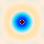
Figure 25: How variable point sources introduce bias. Column 1–2: Simulated ACT (left) and Planck (right) noise-free maps for a single point source. Column 3–4: Each source’s contribution to the coadded map in equation 5, assuming a simple constant-covariance noise model. ACT’s contribution contains a negative shadow that will exactly cancel Planck’s broader beam, resulting in a narrow beam in the final coadd, shown in column 5. If ACT and Planck do not agree on the source’s flux, then this cancellation is not exact, leaving a residual artifact approximately the size of the Planck beam surrounding the source. This is illustrated in column 6 where the source varied in flux by a factor of two between when Planck  and ACT observed it.

When deriving the maximum-likelihood solution for the coadded sky map, we assumed that all individual maps saw different views of a single, consistent sky (see eq. 2). However, this assumption breaks down if the sky changes between the time where the data for the maps was collected, and the central engines of quasars are small enough that their flux can change greatly over time scales of days to months. This is much less than the $\sim 10$ year time-span the data-sets we combine here cover, so we can expect the model to break down in the vicinity of bright, variable quasars.

Figure 25 illustrates how the this modelling error gives rise to artifacts roughly the size of the largest beam involved. A prominent example of this in practice can be seen around the bright, variable quasar PKS 0003-066 in the ACT+Planck map, which is surrounded by a blue shadow with an amplitude of 0.2% of the peak of the source extending about 0.15^∘ away. This relative faintness compared to the source itself explains why this effect is only noticeable around the few brightest and most variable quasars in the map.

For most purposes these rare artifacts can probably be ignored or masked. However, we still provide an alternative version of the coadded maps where a large catalog of point sources were individually fit and subtracted from each input map before they were combined. This was done in two steps:

1. A matched filter point-source finder was run on the standard coadded ACT+Planck day+night maps, resulting in a catalog of 18507/14643/4084 objects detected at more than $5\sigma$ at f090/f150/f220. This corresponds to a flux cut that depends on the local map depth, and is roughly 3.5/3.5/10 mJy in deep regions and 15/15/50 mJy in shallow regions.

2. The flux (but not position) for each source in these catalogs was fit and subtracted in each input map, resulting in source-free maps. During this subtraction, catalog flux measured in the previous step was used as a weak prior. Specifically, the catalog flux entered into the fit as an extra data point, which was assigned a standard deviation $\sigma=\sqrt{\sigma_{F}^{2}+(\alpha F)^{2}}$, where $F$ is the catalog flux and $\sigma_{F}$ is its uncertainty. The second term is there to allow for source variability, with the degree of variability being controlled by the parameter $\alpha$. We set $\alpha=1$ based on it being relatively common for a point source to double in brightness from one season to another.

   The reason for applying a prior was mainly to avoid oversubtracting CMB fluctuations in the Planck maps. The majority of the point sources we subtract are too faint to be detected by Planck. Without a prior, the fit for these would be dominated by the much larger CMB fluctuations, resulting in part of the CMB being subtracted.

The resulting point source subtracted maps were then combined using the same process as the standard maps, resulting in a set of point-source subtracted ACT-only and ACT-Planck  maps.

A limitation of this subtraction process is that it relies on the sources being unresolved points. However, a few nearby galaxies are erroneously detected as point sources. For these, the subtraction process results in incomplete subtraction, and in some cases artifacts that are superficially similar to the ones variable point sources cause in the standard maps. NGC 253 is an example of this.

Appendix C DR4 coadd

In addition to the full 2008-2018 coadded maps, we also provide a “DR4 coadd” that only uses data up to and including ACT DR4 (Aiola et al., 2020) (i.e. 2008-2016). This version contains no f220 data and is 2.3/2.6 times shallower at f090/f150 (in terms of white noise RMS) over most of the map – see figure 14 – but unlike the full version it was not subject to the 3 month post-publication delay, and is available on LAMBDA at https://lambda.gsfc.nasa.gov/product/act/act_dr4_derived_maps_get.cfm as part of ACT DR4.

Appendix D Source code

The Python source code for this analysis is available on Github in the repositories https://github.com/amaurea/enlib and https://github.com/amaurea/tenki. The main coadding code is in enlib/jointmap.py, with the top-level driving script being tenki/auto_coadd2.py. We warn the reader that the implementation is not very clean, and in particular, jointmap.py also contains the implementation of several other unrelated projects. The most relevant parts are Mapset, sanitize_maps, build_noise_model and Coadder.

Appendix E Test on simulated maps

To investigate the noise and bias bias properties of the coadding procedure, we simulated three simple datasets covering a the same $16^{\circ}\times 8^{\circ}$ patch at 0.5 arcmin resolution, but with different beams and noise properties. Dataset 1 and 2 represent ACT-like behavior, with a Gaussian 1.4 arcmin FWHM beam and a low noise floor, but strong noise correlations. Dataset 1 has vertically stripy noise which gradually increases in magnitude towards the left of the image. Dataset 2 has horizontally stripy noise with magnitude instead increasing towards the right. Both have $1/\ell$ noise power spectra with a spectral index of -4.5 and an $\ell_{\textrm{knee}}$ of 3000 in total intensity and 300 in polarization. Dataset 3 represents Planck-like behavior, with a Gaussian 7.0 arcmin FWHM beam and uniform, uncorrelated noise, but on average 10 times higher white noise RMS. We used four different noise realizations for each dataset, resulting in what are effectively 4-way split maps for each of them.

For the signal we used a Gaussian realization of a lensed $\Lambda$CDM power spectrum. This has the advantage of being familiar and reflecting the properties of the real data, but also has the disadvantage of falling rapidly at high $\ell$ due to Silk damping, making it hard to measure bias for $\ell\gtrsim 10\,000$. This could have been avoided by using a simple power law spectrum like $C_{\ell}\propto\ell^{-2}$, but we stuck with $\Lambda$CDM to make the results more intuitive to interpret.

To test for bias, we also made an almost noise-free variant of each dataset. This was done by simply scaling down the noise RMS in the maps by a factor of $50\,000$. Since the noise model used in the coadding procedure only depends on difference maps, the resulting noise models will be identical to those in the normal, noisy case up to a common multiplicative factor, which ultimately cancels when performing the coadd. Hence the low-noise coadd will have exactly the same bias as the normal coadd, but can be measured much more cleanly due to the lack of noise.

We ran the three datasets through the full noise modelling and coadding procedure described in this paper, with the exception that the ground filtering was turned off. The input signal, individual dataset maps and the resulting coadded map are shown in figure 26, and examples of the noise and bias are shown in figure 27. As expected, the coadded map has the best properties of each of the input maps, with the high resolution and low high-$\ell$ noise of dataset 1 and 2, and the low low-$\ell$ noise of dataset 3. What correlated noise is present in the coadd is much more isotropic than the very stripy noise in dataset 1 and 2. No trace of the tile structure is visible.

	T ($\pm 400$µK)	Q ($\pm 40$µK)
Signal
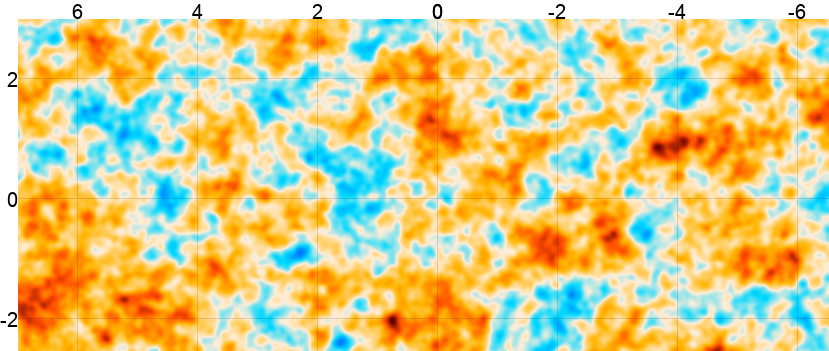
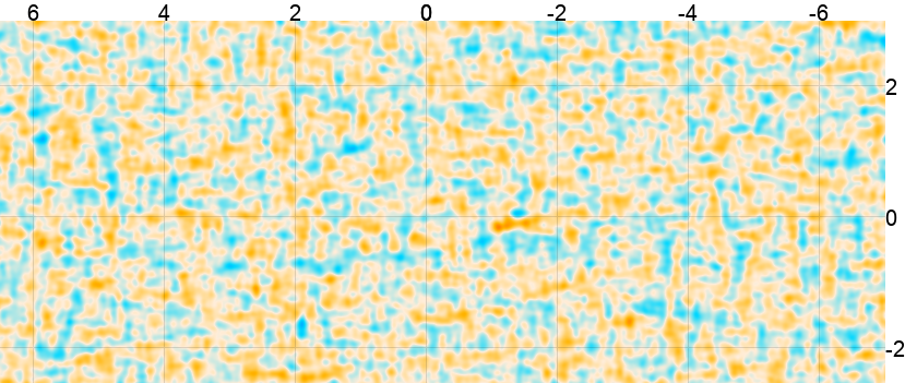
Dataset 1
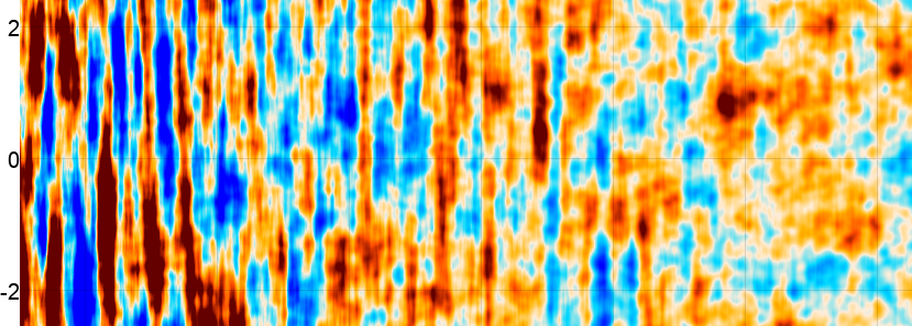
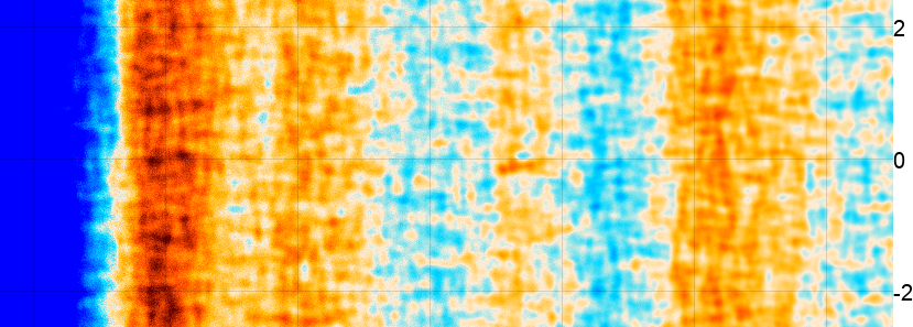
Dataset 2
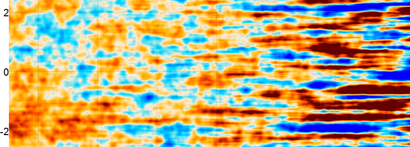
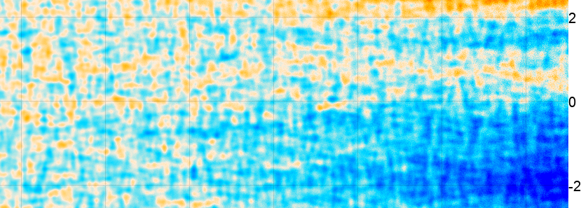
Dataset 3
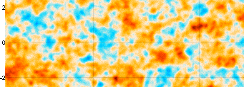
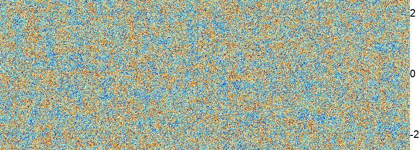
Coadd

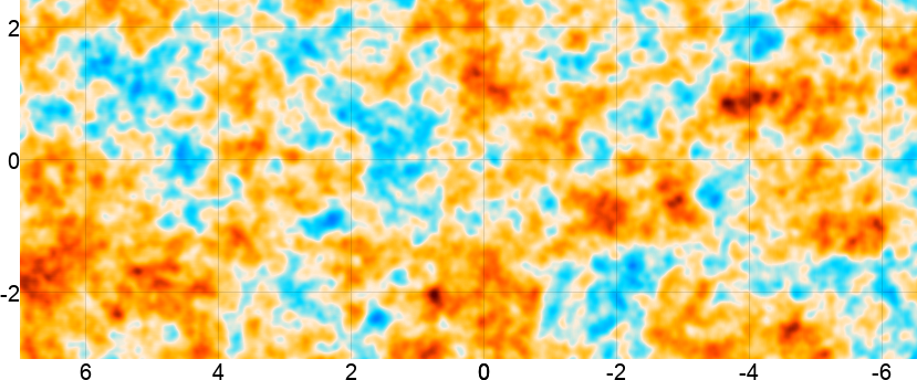
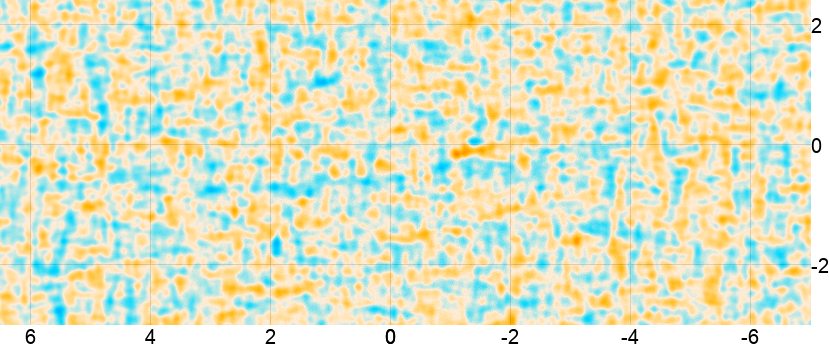
Figure 26: Top: The simulated signal map, smoothed to 1.4 arcmin FWHM resolution. Row 2-4: The mean of the 4 data realizations for dataset 1-3. The spatially dependent stripy noise of the ACT-like datasets 1 and 2 is clearly visible. The Planck-like dataset 3 is 5 times lower resolution and 10 times noisier at high $\ell$, but does not suffer from excess noise at low $\ell$. Bottom: The coadded map combines the best properties of the input datasets. It is high resolution, deep, and has almost no stripy noise. The two columns are total intensity (left) and Stokes-Q (right). Stokes-U would be similar to Stokes-Q, but was left out to save space.

The bias is about 1000 times smaller than the signal, and is caused by the nonzero Conjugate Gradients convergence tolerance. For this test we stopped iteration when the residual variance fell below $10^{-7}$ of the value it had after the first iteration. Lower biases could be achived with a lower tolerance, at a significant performance cost. For the real data coadds we used a higher tolerance of $10^{-4}$, which resulted in much faster convergence while still keeping the bias below 1% of the signal. The excellent signal fidelity and low noise of the coadded map is also visible in the power spectra, as shown in figure 28.

	T ($\pm 400$µK)	Q ($\pm 40$µK)
Coadd noise $\times 10$
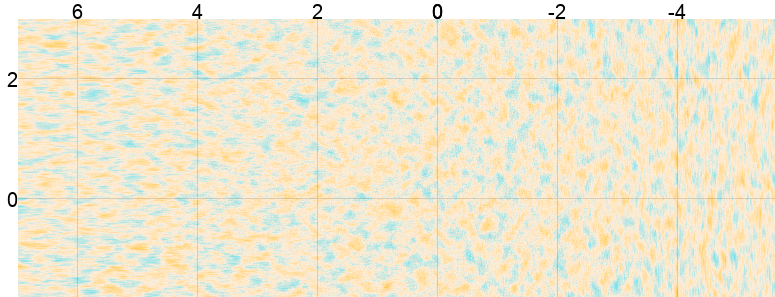
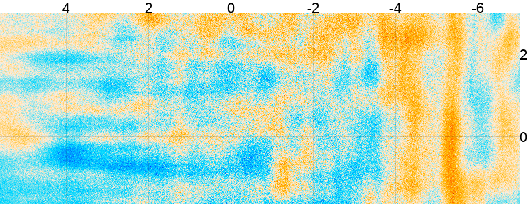
Coadd bias $\times 1000$

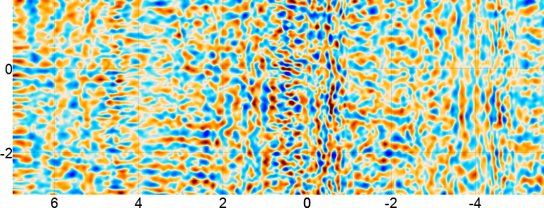
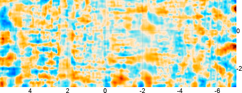
Figure 27: Illustration of the noise and bias properties of the coadded map. Top: The difference between the coadd map and the true signal (i.e. between the bottom and top panel in figure 26), showing the noise properties of the coadd. Scaled by a factor of 10 to make it easier to compare to the signal maps in figure 26. The total intensity (left) noise has almost no stripiness or spatial dependence, unlike the input maps. The polarization noise (right) retains more of the large-scale correlated noise due to dataset 3 being too noisy to help much here. Bottom: The difference between the low-noise coadd map and the true signal, showing the bias properties of the coadd. Scaled by a factor 1000 for visualization purposes.

TT	EE

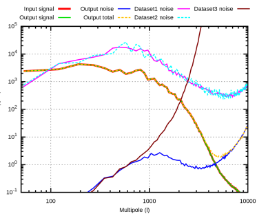
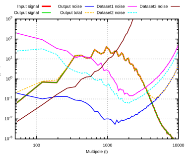
Figure 28: Power spectra of the maps. Left: The TT power spectrum of the true signal (red) is indistinguishable from that of the low-noise coadd (green). The (normal) coadd’s noise power spectrum (blue) is always lower than those of the individual datasets (magenta, cyan and brown). The large improvement in the area dominated by dataset 1 and 2 at $\ell>1000$ is due to the coadd greatly reducing the amount of stripy noise. The yellow curve (output total) is simply the sum of the coadd’s signal and noise power spectra. Right: The EE spectra.

After confirming that the coadding procecure itself has negligible bias, we performed a second run with the ground filter turned on for the ACT-like datasets 1 and 2. We expect this ground cleaning to introduce a bias because it is implemented as a simple filter instead of being incorporated as a weight in the maximum-likelihood framework, and this is confirmed in figure 29, which shows a $\sim$ 0.4% bias for all spectra for $\ell>1000$. At lower $\ell$ this bias falls to 0.05% for TT but grows to up to 10% for EE and BB. This difference is due to filtered datasets 1 and 2 having high noise at low $\ell$ in total intensity, leading to the unfilered dataset 3 dominating there, and hence suppressing the bias.

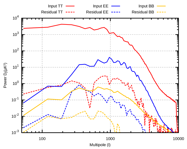
Figure 29: The bias introduced by applying ground filtering to the ACT-like datasets 1 and 2, but not the Planck-like dataset 3. The solid lines show the spectra of the simulated signal. The dashed lines show the residual power, defined as the absolute value of the difference between the power spectra of the simulated map and the output map from the low-noise coadd. TT has low bias on large scales due to the dominance of dataset 3 there, but has a 0.4% power deficiency for $\ell\gtrapprox 2000$. EE and BB behave similarly at high $\ell$, but are more strongly affected for $\ell<1000$ due to the relatively lower weight from the unfiltered dataset 3 there, reaching up to a 10% error at $\ell<350$. These biases can be avoided by replacing simple filtering with maximum-likelihood weighting, which we will do in a future version of these combined maps.

A future version of these maps will replace ground filtering with maximum-likelihood downweighting, which should eliminate this bias, but for now the user should be aware of its presence, which serves as one of the reasons why these maps should not be used for precision cosmology.

References

- Aghanim et al. (2019) Aghanim, N., et al. 2019, arXiv:1902.00350, A&A, 632, A47, PACT
- Aiola et al. (2020) Aiola, S., Calabrese, E., Loic, M., & Naess, S. 2020, ApJS, The Atacama Cosmology Telescope: DR4 Maps and Cosmological Results
- Barentsen et al. (2014) Barentsen, G., et al. 2014, Monthly Notices of the Royal Astronomical Society, 444, 3230–3257, The second data release of the INT Photometric H Survey of the Northern Galactic Plane (IPHAS DR2)
- Bennett et al. (1994) Bennett, C. L., et al. 1994, astro-ph/9401012, ApJ, 436, 423, Cosmic Temperature Fluctuations from Two Years of COBE Differential Microwave Radiometers Observations
- Bennett et al. (2003) —. 2003, astro-ph/0302207, ApJS, 148, 1, First-Year Wilkinson Microwave Anisotropy Probe (WMAP) Observations: Preliminary Maps and Basic Results
- Bennett et al. (2013) —. 2013, arXiv:1212.5225, ApJS, 208, 20, Nine-year Wilkinson Microwave Anisotropy Probe (WMAP) Observations: Final Maps and Results
- Benson et al. (2014) Benson, B. A., et al. 2014, Millimeter, Submillimeter, and Far-Infrared Detectors and Instrumentation for Astronomy VII, SPT-3G: a next-generation cosmic microwave background polarization experiment on the South Pole telescope
- Castelletti et al. (2007) Castelletti, G., Dubner, G., Brogan, C., & Kassim, N. E. 2007, astro-ph/0702746, A&A, 471, 537, The low-frequency radio emission and spectrum of the extended SNR ¡ASTROBJ¿W44¡/ASTROBJ¿: new VLA observations at 74 and 324 MHz
- Choi et al. (2020) Choi, S., Hasselfield, M., Ho, P., Koopman, B., & Lungu, M. 2020, ApJS, ACT DR4
- Chown et al. (2018) Chown, R., et al. 2018, arXiv:1803.10682, ApJS, 239, 10, Maps of the Southern Millimeter-wave Sky from Combined 2500 deg2 SPT-SZ and Planck Temperature Data
- Crawford et al. (2016) Crawford, T. M., et al. 2016, arXiv:1605.00966, ApJS, 227, 23, Maps of the Magellanic Clouds from Combined South Pole Telescope and PLANCK Data
- Das et al. (2011) Das, S., et al. 2011, arXiv:1009.0847, ApJ, 729, 62, The Atacama Cosmology Telescope: A Measurement of the Cosmic Microwave Background Power Spectrum at 148 and 218 GHz from the 2008 Southern Survey
- Datta et al. (2016) Datta, R., et al. 2016, Journal of Low Temperature Physics, 184, 568–575, Design and Deployment of a Multichroic Polarimeter Array on the Atacama Cosmology Telescope
- Dey et al. (2019) Dey, A., et al. 2019, The Astronomical Journal, 157, 168, Overview of the DESI Legacy Imaging Surveys
- Dunkley et al. (2011) Dunkley, J., et al. 2011, arXiv:1009.0866, ApJ, 739, 52, The Atacama Cosmology Telescope: Cosmological Parameters from the 2008 Power Spectrum
- Dünner et al. (2013) Dünner, R., et al. 2013, arXiv:1208.0050, ApJ, 762, 10, The Atacama Cosmology Telescope: Data Characterization and Mapmaking
- Everett et al. (2020) Everett, W. B., et al. 2020, arXiv:2003.03431, Millimeter-wave Point Sources from the 2500-square-degree SPT-SZ Survey: Catalog and Population Statistics
- Fomalont et al. (1989) Fomalont, E. B., Ebneter, K. A., van Breugel, W. J. M., & Ekers, R. D. 1989, ApJ, 346, L17, Depolarization Silhouettes and the Filamentary Structure in the Radio Source Fornax A
- Fomalont et al. (2005) Fomalont, E. B., Ebneter, K. A., van Breugel, W. J. M., Ekers, R. D., Nemiroff, R., & Bonnell, J. 2005, The Giant Radio Lobes of Fornax A, https://apod.nasa.gov/apod/ap050628.html
- Fowler et al. (2007) Fowler, J. W., et al. 2007, astro-ph/0701020, Appl. Opt., 46, 3444, Optical design of the Atacama Cosmology Telescope and the Millimeter Bolometric Array Camera
- Górski et al. (2005) Górski, K. M., Hivon, E., Banday, A. J., Wand elt, B. D., Hansen, F. K., Reinecke, M., & Bartelmann, M. 2005, astro-ph/0409513, ApJ, 622, 759, HEALPix: A Framework for High-Resolution Discretization and Fast Analysis of Data Distributed on the Sphere
- Grace et al. (2014) Grace, E., et al. 2014, Society of Photo-Optical Instrumentation Engineers (SPIE) Conference Series, Vol. 9153, ACTPol: on-sky performance and characterization, 915310
- Gralla et al. (2020) Gralla, M. B., et al. 2020, arXiv:1905.04592, ApJ, 893, 104, Atacama Cosmology Telescope: Dusty Star-forming Galaxies and Active Galactic Nuclei in the Equatorial Survey
- Hasselfield et al. (2013) Hasselfield, M., et al. 2013, arXiv:1303.4714, ApJS, 209, 17, The Atacama Cosmology Telescope: Beam Measurements and the Microwave Brightness Temperatures of Uranus and Saturn
- Henderson et al. (2016) Henderson, S. W., et al. 2016, arXiv:1510.02809, Journal of Low Temperature Physics, 184, 772, Advanced ACTPol Cryogenic Detector Arrays and Readout
- Hilton et al. (2020) Hilton, M., ACT, DES, & HSC. 2020, in preparation, The Atacama Cosmology Telescope: A Catalog of Sunyaev-Zel’dovich Galaxy Clusters
- Madhavacheril et al. (2019) Madhavacheril, M. S., et al. 2019, arXiv:1911.05717, The Atacama Cosmology Telescope: Component-separated maps of CMB temperature and the thermal Sunyaev-Zel’dovich effect
- Meisner et al. (2017) Meisner, A. M., Lang, D., & Schlegel, D. J. 2017, The Astronomical Journal, 154, 161, Deep Full-sky Coadds from Three Years of WISE and NEOWISE Observations
- NASA et al. (2003) NASA, NOAO, ESA, the Hubble Helix Nebula Team, Meixner, M., & Rector, T. 2003, The Iridescent Glory of the Helix Nebula, from Hubble, https://svs.gsfc.nasa.gov/30792
- Planck Collaboration (2013) Planck Collaboration. 2013, arXiv:1303.5062, Planck 2013 results. I. Overview of products and scientific results
- Planck Collaboration (2016a) —. 2016a, arXiv:1502.01582, A&A, 594, A1, Planck 2015 results. I. Overview of products and scientific results
- Planck Collaboration (2016b) —. 2016b, arXiv:1502.01598, A&A, 594, A27, Planck 2015 results. XXVII. The Second Planck Catalogue of Sunyaev-Zeldovich Sources
- Planck Collaboration (2018) —. 2018, arXiv:1807.06205, arXiv e-prints, arXiv:1807.06205, Planck 2018 results. I. Overview and the cosmological legacy of Planck
- Planck Collaboration et al. (2014) Planck Collaboration, et al. 2014, arXiv:1303.5068, A&A, 571, A7, Planck 2013 results. VII. HFI time response and beams
- Planck Collaboration et al. (2016) —. 2016, arXiv:1502.01586, A&A, 594, A7, Planck 2015 results. VII. High Frequency Instrument data processing: Time-ordered information and beams
- Reinecke & Seljebotn (2013) Reinecke, M. & Seljebotn, D. S. 2013, arXiv:1303.4945, A&A, 554, A112, Libsharp - spherical harmonic transforms revisited
- Shewchuk (1994) Shewchuk, J. R. 1994, An Introduction to the Conjugate Gradient Method Without the Agonizing Pain, Tech. rep., USA
- Sievers et al. (2013) Sievers, J. L., et al. 2013, arXiv:1301.0824, J. Cosmology Astropart. Phys, 2013, 060, The Atacama Cosmology Telescope: cosmological parameters from three seasons of data
- Swetz et al. (2011) Swetz, D. S., et al. 2011, arXiv:1007.0290, ApJS, 194, 41, Overview of the Atacama Cosmology Telescope: Receiver, Instrumentation, and Telescope Systems
- Thornton et al. (2016) Thornton, R. J., et al. 2016, arXiv:1605.06569, ApJS, 227, 21, The Atacama Cosmology Telescope: The Polarization-sensitive ACTPol Instrument
- Wright (2007) Wright, N. 2007, The Rosette Nebula as seen in Hydrogen-alpha light, http://www.ing.iac.es/PR/press/rosette.html
- Zaldarriaga & Seljak (1997) Zaldarriaga, M. & Seljak, U. 1997, astro-ph/9609170, Phys. Rev. D, 55, 1830, All-sky analysis of polarization in the microwave background